Neural networks like Long Short-Term Memory (LSTM) recurrent neural networks are able to almost seamlessly model problems with multiple input variables.
This is a great benefit in time series forecasting, where classical linear methods can be difficult to adapt to multivariate or multiple input forecasting problems.
In this tutorial, you will discover how you can develop an LSTM model for multivariate time series forecasting with the Keras deep learning library.
After completing this tutorial, you will know:
How to transform a raw dataset into something we can use for time series forecasting.
How to prepare data and fit an LSTM for a multivariate time series forecasting problem.
How to make a forecast and rescale the result back into the original units.
Kick-start your project with my new book Deep Learning for Time Series Forecasting, including step-by-step tutorials and the Python source code files for all examples.
Let’s get started.
Update Aug/2017: Fixed a bug where yhat was compared to obs at the previous time step when calculating the final RMSE. Thanks, Songbin Xu and David Righart.
Update Oct/2017: Added a new example showing how to train on multiple prior time steps due to popular demand.
Update Sep/2018: Updated link to dataset.
Update Jun/2020: Fixed missing imports for LSTM data prep example.
Tutorial Overview
This tutorial is divided into 4 parts; they are:
Air Pollution Forecasting
Basic Data Preparation
Multivariate LSTM Forecast Model
LSTM Data Preparation
Define and Fit Model
Evaluate Model
Complete Example
Train On Multiple Lag Timesteps Example
Python Environment
This tutorial assumes you have a Python SciPy environment installed. I recommend that youuse Python 3 with this tutorial.
You must have Keras (2.0 or higher) installed with either the TensorFlow or Theano backend, Ideally Keras 2.3 and TensorFlow 2.2, or higher.
The tutorial also assumes you have scikit-learn, Pandas, NumPy and Matplotlib installed.
If you need help with your environment, see this post:
Take my free 7-day email crash course now (with sample code).
Click to sign-up and also get a free PDF Ebook version of the course.
1. Air Pollution Forecasting
In this tutorial, we are going to use the Air Quality dataset.
This is a dataset that reports on the weather and the level of pollution each hour for five years at the US embassy in Beijing, China.
The data includes the date-time, the pollution called PM2.5 concentration, and the weather information including dew point, temperature, pressure, wind direction, wind speed and the cumulative number of hours of snow and rain. The complete feature list in the raw data is as follows:
No: row number
year: year of data in this row
month: month of data in this row
day: day of data in this row
hour: hour of data in this row
pm2.5: PM2.5 concentration
DEWP: Dew Point
TEMP: Temperature
PRES: Pressure
cbwd: Combined wind direction
Iws: Cumulated wind speed
Is: Cumulated hours of snow
Ir: Cumulated hours of rain
We can use this data and frame a forecasting problem where, given the weather conditions and pollution for prior hours, we forecast the pollution at the next hour.
This dataset can be used to frame other forecasting problems.
Do you have good ideas? Let me know in the comments below.
You can download the dataset from the UCI Machine Learning Repository.
Update, I have mirrored the dataset here because UCI has become unreliable:
The first step is to consolidate the date-time information into a single date-time so that we can use it as an index in Pandas.
A quick check reveals NA values for pm2.5 for the first 24 hours. We will, therefore, need to remove the first row of data. There are also a few scattered “NA” values later in the dataset; we can mark them with 0 values for now.
The script below loads the raw dataset and parses the date-time information as the Pandas DataFrame index. The “No” column is dropped and then clearer names are specified for each column. Finally, the NA values are replaced with “0” values and the first 24 hours are removed.
The “No” column is dropped and then clearer names are specified for each column. Finally, the NA values are replaced with “0” values and the first 24 hours are removed.
Running the example creates a plot with 7 subplots showing the 5 years of data for each variable.
Line Plots of Air Pollution Time Series
3. Multivariate LSTM Forecast Model
In this section, we will fit an LSTM to the problem.
LSTM Data Preparation
The first step is to prepare the pollution dataset for the LSTM.
This involves framing the dataset as a supervised learning problem and normalizing the input variables.
We will frame the supervised learning problem as predicting the pollution at the current hour (t) given the pollution measurement and weather conditions at the prior time step.
This formulation is straightforward and just for this demonstration. Some alternate formulations you could explore include:
Predict the pollution for the next hour based on the weather conditions and pollution over the last 24 hours.
Predict the pollution for the next hour as above and given the “expected” weather conditions for the next hour.
We can transform the dataset using the series_to_supervised() function developed in the blog post:
First, the “pollution.csv” dataset is loaded. The wind direction feature is label encoded (integer encoded). This could further be one-hot encoded in the future if you are interested in exploring it.
Next, all features are normalized, then the dataset is transformed into a supervised learning problem. The weather variables for the hour to be predicted (t) are then removed.
Running the example prints the first 5 rows of the transformed dataset. We can see the 8 input variables (input series) and the 1 output variable (pollution level at the current hour).
This data preparation is simple and there is more we could explore. Some ideas you could look at include:
One-hot encoding wind direction.
Making all series stationary with differencing and seasonal adjustment.
Providing more than 1 hour of input time steps.
This last point is perhaps the most important given the use of Backpropagation through time by LSTMs when learning sequence prediction problems.
Define and Fit Model
In this section, we will fit an LSTM on the multivariate input data.
First, we must split the prepared dataset into train and test sets. To speed up the training of the model for this demonstration, we will only fit the model on the first year of data, then evaluate it on the remaining 4 years of data. If you have time, consider exploring the inverted version of this test harness.
The example below splits the dataset into train and test sets, then splits the train and test sets into input and output variables. Finally, the inputs (X) are reshaped into the 3D format expected by LSTMs, namely [samples, timesteps, features].
1
2
3
4
5
6
7
8
9
10
11
12
13
...
# split into train and test sets
values=reframed.values
n_train_hours=365*24
train=values[:n_train_hours,:]
test=values[n_train_hours:,:]
# split into input and outputs
train_X,train_y=train[:,:-1],train[:,-1]
test_X,test_y=test[:,:-1],test[:,-1]
# reshape input to be 3D [samples, timesteps, features]
Running this example prints the shape of the train and test input and output sets with about 9K hours of data for training and about 35K hours for testing.
1
(8760, 1, 8) (8760,) (35039, 1, 8) (35039,)
Now we can define and fit our LSTM model.
We will define the LSTM with 50 neurons in the first hidden layer and 1 neuron in the output layer for predicting pollution. The input shape will be 1 time step with 8 features.
We will use the Mean Absolute Error (MAE) loss function and the efficient Adam version of stochastic gradient descent.
The model will be fit for 50 training epochs with a batch size of 72. Remember that the internal state of the LSTM in Keras is reset at the end of each batch, so an internal state that is a function of a number of days may be helpful (try testing this).
Finally, we keep track of both the training and test loss during training by setting the validation_data argument in the fit() function. At the end of the run both the training and test loss are plotted.
After the model is fit, we can forecast for the entire test dataset.
We combine the forecast with the test dataset and invert the scaling. We also invert scaling on the test dataset with the expected pollution numbers.
With forecasts and actual values in their original scale, we can then calculate an error score for the model. In this case, we calculate the Root Mean Squared Error (RMSE) that gives error in the same units as the variable itself.
NOTE: This example assumes you have prepared the data correctly, e.g. converted the downloaded “raw.csv” to the prepared “pollution.csv“. See the first part of this tutorial.
Running the example first creates a plot showing the train and test loss during training.
Note: Your results may vary given the stochastic nature of the algorithm or evaluation procedure, or differences in numerical precision. Consider running the example a few times and compare the average outcome.
Interestingly, we can see that test loss drops below training loss. The model may be overfitting the training data. Measuring and plotting RMSE during training may shed more light on this.
Line Plot of Train and Test Loss from the Multivariate LSTM During Training
The Train and test loss are printed at the end of each training epoch. At the end of the run, the final RMSE of the model on the test dataset is printed.
We can see that the model achieves a respectable RMSE of 26.496, which is lower than an RMSE of 30 found with a persistence model.
1
2
3
4
5
6
7
8
9
10
11
12
...
Epoch 46/50
0s - loss: 0.0143 - val_loss: 0.0133
Epoch 47/50
0s - loss: 0.0143 - val_loss: 0.0133
Epoch 48/50
0s - loss: 0.0144 - val_loss: 0.0133
Epoch 49/50
0s - loss: 0.0143 - val_loss: 0.0133
Epoch 50/50
0s - loss: 0.0144 - val_loss: 0.0133
Test RMSE: 26.496
This model is not tuned. Can you do better?
Let me know your problem framing, model configuration, and RMSE in the comments below.
Train On Multiple Lag Timesteps Example
There have been many requests for advice on how to adapt the above example to train the model on multiple previous time steps.
I had tried this and a myriad of other configurations when writing the original post and decided not to include them because they did not lift model skill.
Nevertheless, I have included this example below as reference template that you could adapt for your own problems.
The changes needed to train the model on multiple previous time steps are quite minimal, as follows:
First, you must frame the problem suitably when calling series_to_supervised(). We will use 3 hours of data as input. Also note, we no longer explictly drop the columns from all of the other fields at ob(t).
1
2
3
4
5
6
...
# specify the number of lag hours
n_hours=3
n_features=8
# frame as supervised learning
reframed=series_to_supervised(scaled,n_hours,1)
Next, we need to be more careful in specifying the column for input and output.
We have 3 * 8 + 8 columns in our framed dataset. We will take 3 * 8 or 24 columns as input for the obs of all features across the previous 3 hours. We will take just the pollution variable as output at the following hour, as follows:
The only other small change is in how to evaluate the model. Specifically, in how we reconstruct the rows with 8 columns suitable for reversing the scaling operation to get the y and yhat back into the original scale so that we can calculate the RMSE.
The gist of the change is that we concatenate the y or yhat column with the last 7 features of the test dataset in order to inverse the scaling, as follows:
1
2
3
4
5
6
7
8
9
10
...
# invert scaling for forecast
inv_yhat=concatenate((yhat,test_X[:,-7:]),axis=1)
inv_yhat=scaler.inverse_transform(inv_yhat)
inv_yhat=inv_yhat[:,0]
# invert scaling for actual
test_y=test_y.reshape((len(test_y),1))
inv_y=concatenate((test_y,test_X[:,-7:]),axis=1)
inv_y=scaler.inverse_transform(inv_y)
inv_y=inv_y[:,0]
We can tie all of these modifications to the above example together. The complete example of multvariate time series forecasting with multiple lag inputs is listed below:
Note: Your results may vary given the stochastic nature of the algorithm or evaluation procedure, or differences in numerical precision. Consider running the example a few times and compare the average outcome.
The model is fit as before in a minute or two.
1
2
3
4
5
6
7
8
9
10
11
12
13
...
Epoch 45/50
1s - loss: 0.0143 - val_loss: 0.0154
Epoch 46/50
1s - loss: 0.0143 - val_loss: 0.0148
Epoch 47/50
1s - loss: 0.0143 - val_loss: 0.0152
Epoch 48/50
1s - loss: 0.0143 - val_loss: 0.0151
Epoch 49/50
1s - loss: 0.0143 - val_loss: 0.0152
Epoch 50/50
1s - loss: 0.0144 - val_loss: 0.0149
A plot of train and test loss over the epochs is plotted.
Plot of Loss on the Train and Test Datasets
Finally, the Test RMSE is printed, not really showing any advantage in skill, at least on this problem.
hello Jason,
I have run the code in my spyder and I know the RMSE index is good enough for this model. However, I added the accuracy index in this code, that is
model.compile(loss=’mae’, optimizer=’adam’, metrics=[‘accuracy’])
and the accuracy is totally the same in each epoch and is very low (0.0761). I also use my own data to run your code, and the result is the same, with good RMSE values but bad accuracy. I have troubled by this for several days and looking forward to your reply.
Hi,Jason.
I have the same problem as qing.I don‘t know why we cannot measure accuracy for regression.And the website you provided cannot be opened.
Could you please help me with that?
hi,Jason,I‘m a new learner. There is no real curve and predicted curve in your tutorial.
I want to know how can I get it? I mean how to write it in the code?
To predict the next three months’ data for all daily intervals excluding weekends using multivariate time series forecasting with LSTMs in Keras, you can follow these steps:
—
### 1. **Understand the Data**
– Ensure your dataset has **features (independent variables)** and a **target variable** to predict.
– Ensure the dataset has time indices and does not include weekends for both training and predictions.
—
### 2. **Prepare the Dataset**
1. **Filter Out Weekends:**
– Use the pandas library to filter out rows with weekend dates. python
import pandas as pd
# Assume 'date' is your timestamp column
df['date'] = pd.to_datetime(df['date'])
df = df[~df['date'].dt.weekday.isin([5, 6])] # Exclude Saturdays and Sundays
2. **Scale Features:**
– Normalize or standardize the features for better LSTM performance. python
from sklearn.preprocessing import MinMaxScaler
3. **Create Input Sequences:**
– LSTMs require sequential data. Create sequences for a rolling window. python
def create_sequences(data, seq_length):
X, y = [], []
for i in range(len(data) - seq_length):
X.append(data[i:i+seq_length, :-1]) # All features except the target
y.append(data[i+seq_length, -1]) # The target variable
return np.array(X), np.array(y)
seq_length = 30 # Example: Use 30 past days to predict the next day
X, y = create_sequences(scaled_data, seq_length)
—
### 3. **Build the LSTM Model** python
from keras.models import Sequential
from keras.layers import LSTM, Dense
model = Sequential([
LSTM(128, return_sequences=True, input_shape=(X.shape[1], X.shape[2])),
LSTM(64),
Dense(32, activation='relu'),
Dense(1) # Predicting one value
])
model.compile(optimizer='adam', loss='mse')
—
### 4. **Train the Model** python
history = model.fit(X, y, epochs=50, batch_size=32, validation_split=0.2, shuffle=False)
—
### 5. **Make Predictions for the Next Three Months**
1. **Prepare Future Input Data:**
– Start with the last known data points and iterate to predict the next day, using each prediction as input for subsequent predictions. python
import numpy as np
for _ in range(days_to_forecast):
pred = model.predict(input_seq[np.newaxis, :, :])[0, 0]
predictions.append(pred)
# Update the input sequence with the new prediction
input_seq = np.vstack([input_seq[1:], np.append(input_seq[-1, :-1], pred)])
return predictions
2. **Generate Future Dates Excluding Weekends:**
– Calculate future dates without weekends. python
from datetime import timedelta
last_date = df['date'].max()
future_dates = []
while len(future_dates) < days_to_forecast:
last_date += timedelta(days=1)
if last_date.weekday() not in [5, 6]: # Skip weekends
future_dates.append(last_date)
3. **Generate Predictions:**
- Use the forecast_future function to predict daily intervals and map them to future dates. python
last_input = scaled_data[-seq_length:, :] # Use the last known input sequence
predictions = forecast_future(model, last_input, len(future_dates))
### 6. **Validate the Model**
- Use a separate validation dataset to check the accuracy of your model.
- Consider tuning hyperparameters or using advanced architectures like Seq2Seq or attention mechanisms if accuracy is unsatisfactory.
---
### 7. **Plot the Results** python
import matplotlib.pyplot as plt
Many thanks for this incredibly useful example!
I think I might have a small suggestion: I’ve downloaded the “pollution” data set from the Github link provided, and I found out that maybe the column to be encoded is now column 8 and not 4 like in the original code, so I made this amendment and it all worked: (apologies if I’m missing something):
# I’ve replaced this line:
#values[:,4] = encoder.fit_transform(values[:,4])
# … with this line:
values[:,8] = encoder.fit_transform(values[:,8])
But make sure instead of 7 you use number_of_features -1, otherwise you have the value error.
So in my case, I use 31 features (including the one I wanna predict), and it is the following code:
inv_yhat = concatenate((yhat, test_X[:, -30:]), axis=1)
as well as for inv_y:
inv_y = concatenate((test_y, test_X[:, -30:]), axis=1)
It seems that inv_y = scaler.inverse_transform(test_X)[:,0] is not the actual, should inv_yhat be compared with test_y but not pollution(t-1)? Because I think this inv_y here means pollution(t-1). Is this prediction equals to only making a time shifting from the current known pollution value (which means the models just take pollution(t) as the prediction of pollution(t+1))?
Sorry for the confusing expression. In fact, the series_to_supervised() function would create a DataFrame whose columns are: [ var1(t-1), var2(t-1), …, var1(t) ] where ‘var1’ represents ‘pollution’, therefore, the first dimension in test_X (that is, test_X[:,0]) would be ‘pollution(t-1)’. However, in the code you calculate the rmse between inv_yhat and test_X[:,0], even though the rmse is low, it could only shows that the model’s prediction for t+1 is close to what it has known at t.
I am asking this question because I’ve ran through the codes and saw the models prediction pollution(t+1) looks just like pollution(t). I’ve also tried to use t-1, t-2 and so on for training, but still changed nothing.
Do you think the model tends to learn to just take the pollution value at current moment as the prediction for the next moment?
In a word, and also it’s an example, I want to ask two questions:
1. In the “make a prediction” part of your codes, why it computes rmse between predicted t+1 and real t, but not between predicted t+1 and real t+1?
2. After the “make a prediction” part of your codes run, it turns out that rmse between predicted t+1 and real t is small, is it an evidence that LSTM is making persistence?
I think Songbin Xu is right. By executing the statement at line 90: inv_y = inv_y[:,0], you compare the inv_yhat with inv_y. inv_y is the polution(t-1) and inv_yhat is the predicted polution(t).
On line 50 the second parameter the function series_to_supervised can be changed to 3 or 5, so more days of history are used. If you do so, an error occurs in the scaler.inverse_transform (line 89).
No worries, great tutorial and I learned a lot so far!
I have updated the calculation of RMSE and the final score reported in the post.
Note, I ran a ton of experiments on AWS with many different lag values > 1 and none achieved better results than a simple lag=1 model (e.g. an LSTM model with no BPTT). I see this as a bad sign for the use of LSTMs for autoregression problems.
As for this:
Updated Aug/2017: Fixed a bug where yhat was compared to obs at the previous time step when calculating the final RMSE. Thanks, Songbin Xu and David Righart.
It seems to have some errors on calculating RMSE based on (t-1) vs (t) different time slots before. I’m just curious how it is corrected? Can you elaborate that little bit more? Because for me, I’m still thinking it is RMSE based on (t-1) vs (t)
hey,Janson.The RMSE before you updated it was 3.386. Is this article RMSE 26.496 the correct answer after you updated it? In other words,inv_y = scaler.inverse_transform(test_X)[:,0] is not true,test_y = test_y.reshape((len(test_y), 1))
inv_y = concatenate((test_y, test_X[:, 1:]), axis=1)
inv_y = scaler.inverse_transform(inv_y) is the correct code,is it right?I find so many people use the incorrect code .
Thank you for an awesome post.
(I was practicing on load forecast using MLP and SVR (You also suggested on a comment in your other LSTM tutorials). I also tried with LSTM and it did almost perform like SVR. However, in LSTM, I did not consider time lags because I have predicted future predictor variables that I was feeding as test set. I will try this method with time lags to cross validate the models)
Can I use ‘look back'(Using t-2 , t-1 steps data to predict t step air pollution) in this case?
If it’s available,that my input data shape will be [samples , look back , features] isn’t it?
If I used n_in=5 in series_to_supervised() function,in your tutorial the input shape will be [samples, 1 , features*5].Can I reshape it to [samples, 5 , features]?If I can, what is the difference between these two shape?
The second dimension is time steps (e.g. BPTT) and the third dimension are the features (e.g. observations at each time step). You can use features as time steps, but it would not really make sense and I expect performance to be poor.
Here’s how to build a model multiple time steps for multiple features:
Jason, great post, very clear, and very useful!! I’m about 90% with you and think a few folks may be stuck on this final point if they try to implement multi-feature, multi-hour-lookback LSTM.
Seems like by making adjustments above, I’m able to make a prediction, but the scaling inversion doesn’t want to cooperate. The reshape step now that we have multiple features and multiple timesteps has a mismatch in the shape, and even if I make the shape work, the concatenation and inversion still don’t work. Could you share what else you changed in this section to make it work? I’m not so concerned about the RMSE as much as that I can extract useful predictions. Thank you for any insight since you’ve been able to do it successfully.
# make a prediction
yhat = model.predict(test_X)
test_X = test_X.reshape((test_X.shape[0], test_X.shape[2]))
# invert scaling for forecast
inv_yhat = concatenate((yhat, test_X[:, 1:]), axis=1)
inv_yhat = scaler.inverse_transform(inv_yhat)
inv_yhat = inv_yhat[:,0]
I am somewhat puzzled by the number of features you specify to forecast the pollution rate based on data from the previous 24 hours.
Do not we have 8 features for each time-step and not 7?
After generating data to supervise with the function series_to_supervised(scaled,24, 1), the resulting array has a shape of (43800, 200) which is 25 * 8.
To invert the scaling for forecast I made few modifications. I used scaled.shape[1] below but in my opinion it could be n_features. Moreover, I don’t know if the values concatenated to yhat and test_y really matter, as long as they have been scaled with fit_transform and the array has the right shape.
Date and wind direction are dropped during data preparation, perhaps you accidentally skipped a step or are reviewing a different file from the output file?
When reading the file, the field ‘date’ becomes the index of the dataframe and the field ‘wnd_dir’ is later label encoded, as you do above in “The complete example” lines 42-43.
It is now much clearer for me. I am not puzzled anymore. 😉
Thanks a lot for all the information contained in your articles and your e-books.
Hi Jason,
I think the output is column var1(t), that means:
train_X, train_y = train[:, 0:n_obs], train[:, -(n_features+1)]
am I right?
In case the “pollution” is in the last column, it is easy to get train[:, -1]
am i right?
I just want to verify that I understand your post.
Thank you, Jason
I want to use a bigger windows (I want to go back in time more, for example t-5 to include more data to make a prediction of the time t) and use all of this to predict one variable (such as just the pollution), like you did. I think predicting one variable will be more accurate than predicting many. Such as pollution and temperature.
First of all, thanks for your work and the effort you put in!
I tried to implement your suggestion for increasing the timesteps (BPTT). I have intergrated your code but I keep getting this error in when reshaping test_X in the prediction step:
test_X = test_X.reshape((test_X.shape[0], test_X.shape[2]))
ValueError: cannot reshape array of size 490532 into shape (35038,7)
Hi,Janson.I am a new leaner. First, thank fou for your share! But, when I run the complete code, it has an error: pyplot.plot(history.history[‘val_loss’], label=’test’)
KeyError: ‘val_loss’
Hi Jason,
Thank you for this excellent tutorial. I recently started working on LSTM methods. I have a doubt regarding this input shape. In case if the n_hour >1 , how to inverse transform the scaled values? Thanks in advance. Thanks in advance.
Hi Jason, I get the following error from line # 82 of your ‘Complete Example’ code.
ValueError: Error when checking : expected lstm_1_input to have 3 dimensions, but got array with shape (34895, 8)
I think LSTM() is looking for (sequences, timesteps, dimensions). In your code, line # 70, I believe 50 is timesteps while input_shape (1,8) represents the dimensions. May be it’s missing ‘sequences’ ?
Hi Jason, I am wondering what the issue that I’m getting is caused by, maybe a different type of dataset then the example one. basically when I run the history into the model, When i check the History.history.keys() I only get back ‘loss’ as my only key.
If you replace in this example the target by a binary target, let us say one that says if the var_1 goes up or not in the next move, thus : :
reframed[‘var1(t)_diff’]=reframed[‘var1(t)’].diff(1)
reframed[‘target_diff’]=reframed[‘var1(t)_diff’].apply(lambda x : (x>0)*1)
it gives this error :
””
You are passing a target array of shape (8760, 1) while using as loss categorical_crossentropy. categorical_crossentropy expects targets to be binary matrices (1s and 0s) of shape (samples, classes). If your targets are integer classes, you can convert them to the expected format via:
””’
which was :
X = dataset[:,0:8]
Y = dataset[:,8]
model = Sequential()
model.add(Dense(12, input_dim=8, activation=’relu’))
model.add(Dense(8, activation=’relu’))
model.add(Dense(1, activation=’sigmoid’))
model.compile(loss=’binary_crossentropy’, optimizer=’adam’, metrics=[‘accuracy’])
model.fit(X, Y, epochs=150, batch_size=10)
it gives no error whereas the Y have the same shape … why ?
How can we make it work for the lstm classification please ?
But
trainy_postcategorical = to_categorical(trainy)
trainy_postcat.shape
gives
print(trainy_postcat.shape)
(7352, 7)
which means one additional variable has been created while we were expecting 6 dummies only.
pd.DataFrame(trainy_postcat)[0].sum() gives 0 so empty column for 1st one
Come back to the sahpe of lstm.
the output of your pre process work gives :
trainy_postcat.shape
Out[219]: (7352, 7)
which for a single dummy (the case of this article and my original question)
is the analogy of
”’ You are passing a target array of shape (8760, 1) ”
which should be good.
Any idea ? the activity recognition analogy does not solve the shape issue.
Since you have published a similar topic and few other related topics in one of your paid books (LSTM networks), should the reader also expect some different topics covered in it?
I’m an ardent fan of your blogs since it covers most of the learning material and therefore, it makes me wonder that will be different in your book?
The book does not cover time series, instead it focuses on teaching you how to implement a suite of different LSTM architectures, as well as prepare data for your problems.
Some ideas were tested on the blog first, most are only in the book.
The book provides all the content in one place, code as well, more access to me, updates as I fix bugs and adapt to new APIs, and it is a great way to support my site so I can keep doing this.
Thank you for accepting my opinions, such a pleasure!
Running the codes u modified, still something puzzles me here,
1. Have u drawn the waveforms of inv_y and inv_yhat in the same plot? I think they looks quite like persistence.
2. Curiously, I computed the rmse between pollution(t) and pollution(t-1) in test_X, it’s 4.629, much lower than your final score 26.496, does it mean LSTM performs even worse than persistence?
3. I’ve tried to remove var1 at t-1, t-2, … , and I’ve also tried to use lag values>1, and also assign different weights to the inputs at different timesteps, but none of them improved, they performed even worse.
Do you have any other ideas to avoid the whole model to learn persistence?
When the timesteps = 1 as you mentioned, does it mean the value of t-1 time was used to predict the value of t time? Is moving window a method to use multiple time steps? Is there any other way? Has Keras any functions of moving window?
Hi Jason, Its a very Informative article. Thanks. I have a question regarding forecasting in time series. You have used the training data with all the columns while learning after variable transformations and the same has been done for the test data too. The test data along with all the variables were used during prediction. For instance, If I want to predict the pollution for a future date, Should I know the other inputs like dew, pressure, wind dir etc on a future date which I’m not aware off? Another question is, Suppose we have same data about multiple regions(let us consider that the pollution among these regions is not negligible), How can we model so that the input argument while prediction is the region name along with time to forecast just for that one region.
The model defined above uses the variables from the prior time step as inputs to predict the next pollution value.
In your case, maybe you want to build a separate model per region, perhaps a model that improves performance by combining models across regions. You must experiment to see what works best for your data.
Thanks! I missed the trick of converting the time-series to supervised learning problem. That alone is sufficient even for multiple regions I guess. We just have to submit the input parameters of the previous time stamp for the specific region during prediction. We may also try one-hot encoding on the region variable too during data preprocessing.
Thank you for your excellent blog, Jason. I’ve really learnt a lot from your nice work recently. After this post, I’ve already known how to transform data into data that formates LSTM and how to construct a LSTM model.
Like the question aksed by Naveen Koneti, I have the same puzzle.
Recently I’ve worked on some clinical data. The data is not like the one we used in this demo. It is consist of hunderds of patients, each patient has several vital sign records. If it is about one individual’s records through many years, I can process the data as what you told us. I wonder how I can conquer this kind of data. Could you give me some advice, or tell me where I can find any solutions about it?
If I didn’t state my question clearly and you’re interested it, pls let me know.
Thanks in advance.
PS. the data set in my situation is like this
[ID date feature1 feature2 feautre3 ]
[patient1 date1 value11 value12 value13 ]
[patient1 date2 value21 value22 value23 ]
[patient2 date1 value31 value32 value33 ]
[patient2 date2……………………………………..]
[patient3 ……………………………………………..]
Hi Naveen, I have the same your question: the model is defined such that if you know the input features at time t, then you can predict the target value at time t+1. If you want to predict the target variable at time t+2, though, you would need to know the input features at time t+1. If a feature does not change over time, it is no problem; but if a feature changes over time, then its value at time t+1 is not known and may be different from its value at time t.
I am thinking that to solve this, you would need to define such features as output of the model as well as the target variable. In this way, at time t, you can predict the target variable for time t+1, but also the feature for time t+1, so that this predicted value can be used as input to predict the target variable for time t+2.
What do you think about that? Did you think of a different solution?
Many thanks
I would like to build a network, in which each feature has its own LSTM neuron/layer, so that the input is not fully connected.
My idea is adding a lstm layer for each feature and merge it with the merge layer and feed these results to the output neurons.
Is there a better way to do this? Or would you recommend to avoid this because the features are poorly abstracted? On the other hand, this might also be interesting.
1) I have a question/ notice regarding the scaling of the Y variable (pollution). The way you implement the rescaling between [0-1] you consider the entire length of the array (all of the 43799 observations -after the dropna-).
Is it rightto rescale it that way? By doing so we are incorporating information of the furture (test set) to the past (train set) because the scaler is “exposed” to both of them and therefore we introduce bias.
If you agree with my point what could be a fix?
2) Also the activation function of the output (Y variable) is sigmoid, that’s why we rescale it within the [0,1] range. Am I correct?
First I wanna thanks for your helpful and practical blog.
I tried to separate train and test set to do normalization on training but I have gotten error related to test set shape something like that “ValueError: cannot reshape array of size 136 into shape (34,2,4)”, which I don’t know how to fix it!
Do you have an example on LSTM which run normalization on train and used in test, or do you explain that in your book?
I did some changes and just use transform method on test set, is that correct?
firstly I divided my data-set to two different sets ,(train and test)
secondly I ran fit_transform on train set and transform on test set
But I get rmse=0 ? which seems weird. am I correct?
You have to prepare the Data befor you convert (see “Basic Data Preparation”). In Jason’s complete Example of the LSTM this preparation step is missing (more likely left out).
Yes the note above the complete example says clearly:
NOTE: This example assumes you have prepared the data correctly, e.g. converted the downloaded “raw.csv” to the prepared “pollution.csv“. See the first part of this tutorial.
I agree with @Dmitry here. The prediction “inv_yhat” is one index ahead of real output “inv_y”.
It can be seen by plotting predicted output v/s real output:
pyplot.plot(inv_y[:-1,], color=’green’, marker=’o’, label = ‘Real Screening Count’)
pyplot.plot(inv_yhat[1:,], color=’red’, marker=’o’, label = ‘Predicted Screening Count’)
pyplot.legend()
pyplot.show()
Compute RMSE by skipping first element of inv_yhat, and better RSME score is presented:
rmse = sqrt(mean_squared_error(inv_y[:-1,], inv_yhat[1:,]))
print(‘Test RMSE: %.3f’ % rmse)
great post! I was waiting for meteo problems to infiltrate the machinelearningmastery world.
Could you write something about the changed scenareo where, given the weather conditions and pollution for some time, we can predict the pollution for another time or place with given weather conditions?
For example: We have the weather conditions and pollution given for Beijing in 2016, and we have the weather conditions given for Chengde (city close to Bejing) also in 2016. Now we want to know how was the pollution in Chengde in 2016.
Hi Jason,
I have read many of your posts about LSTM. I have not completely clear the difference between the parameters batch_size and time_steps. Batch_size means when the memory is reset (right?), but this shouldn’t have the same value of time_steps that, if I have understood correctly, means how often the system makes a prediction?
Batch size is the number of samples (e.g. sequences) to that are used to estimate the gradient before the weights are updated. The internal state is reset at the end of each batch after the weights are updated.
One sample is comprised of 1 or more time steps that are stepped over during backpropagation through time. Each time step may have one or more features (e.g. observations recorded at that time).
Time steps and batch size and generally not related.
You can split up a sequence to have one-time step per sequence. In that case you will not get the benefit of learning across time (e.g. bptt), but you can reset state at the end of the time steps for one sequence. This an odd config though and really only good to showing off the LSTMs memory capability.
C:\Anaconda3\lib\site-packages\keras\models.py in add(self, layer)
431 # and create the node connecting the current layer
432 # to the input layer we just created.
–> 433 layer(x)
434
435 if len(layer.inbound_nodes) != 1:
C:\Anaconda3\lib\site-packages\keras\layers\recurrent.py in __call__(self, inputs, initial_state, **kwargs)
241 # modify the input spec to include the state.
242 if initial_state is None:
–> 243 return super(Recurrent, self).__call__(inputs, **kwargs)
244
245 if not isinstance(initial_state, (list, tuple)):
C:\Anaconda3\lib\site-packages\keras\engine\topology.py in __call__(self, inputs, **kwargs)
556 ‘layer.build(batch_input_shape)‘)
557 if len(input_shapes) == 1:
–> 558 self.build(input_shapes[0])
559 else:
560 self.build(input_shapes)
C:\Anaconda3\lib\site-packages\tensorflow\python\framework\ops.py in convert_to_tensor(value, dtype, name, as_ref, preferred_dtype)
667
668 if ret is None:
–> 669 ret = conversion_func(value, dtype=dtype, name=name, as_ref=as_ref)
670
671 if ret is NotImplemented:
Hi Jason, I did have an issue converting back to actual values, but was able to get past it using the drop columns on the reframed data which got me past it.
When looking at my predicted values vs actual values, I’m noticing that my first column has a prediction and a true value, but for every other variable, I only see what I can assume is a prediction? does this make a prediction on every column, or just one particular one.
Im sorry for asking a question such as this, I just think I’m confusing myself looking at my results.
Dr. Jason,
I have been trying with my own dataset and I am getting an error “ValueError: operands could not be broadcast together with shapes (168,39) (41,) (168,39)” when I try to do inv_yhat = scaler.inverse_transform(inv_yhat) as you have in line 86 in your script. I still can not figure out where my issue is. I have yhat.shape as (168,1) and test_X.shape as (168,38). When I do this, inv_yhat = np.concatenate((yhat, test_X[:, 1:]), axis=1), my inv_yhat.shape is (168,39). I still can not figure why inverse_transform gives that error.
The shape of the data must be the same when inverting the scale as when it was originally scaled.
This means, if you scaled with the entire test dataset (all columns), then you need to tack the yhat onto the test dataset for the inverse. We jump through these exact hoops at the end of the example when calculating RMSE.
This seems to be the same issue I am having at the moment also. i concatenate my inv_yhat with my test_X like you said, but the shape of inv_yhat after is still not taking into account the 2nd numbers(in posts case (41,).
I am having the same problem, but cannot solve the issue. everytime i try to concatenante them together, there is not change to my inv_yhat variable. i still am unable to understand this issue if you can expand a bit more that would be amazing
@John Regilina,
Check the shape of data after you scale the data and then check the scale again after you do the concatenation. Remember, when your yhat shape will be (rowlength,1) and after concatenation inv_yhat should be the same shape after you scaled the data. Look at Dr.Jason’s answer to my comment/question. Hope that will help. (Thanks to Dr.Jason saved a lot of my time)
Hello Sir, thank you for the awesome tutorial. But I still couldn’t understand what exactly needs to be done. I am getting the error:
> operands could not be broadcast together with shapes (12852,27) (14,) (12852,27) ”
This the line which generates the error:
inv_yhat = scaler.inverse_transform(inv_yhat).fit()
Could you please give me a small example to understand what went wrong. Thanks in advance Sir.
I am suffering from the same problem when i am trying it on my dataset having np.shape(test_X) as (89070,13) size. Kindly kindly help me out if you have got the solution.
We specify to remove the column with axis=1 and to do it on the array in memory with inplace rather than return a copy of the array with the column removed.
Jason, what am I missing, looking at your plot of the most recent 100 time steps, it looks like the predicted value is always 1 time period after the actual? If on step 90 the actual is 17, but the predicted value shows 17 for step 91, we are one time period off, that is if we shifted the predicted values back a day, it would overlap with the actual which doesn’t really buy us much since the next hour prediction seems to really align with the prior actual. Am I missing something looking at this chart?
So how would you get the true predicted value(t)? I am thinking of the last record in the time series where we are trying to predict the value for the next hour.
Thank you for your great posts. I run the model above for my data and it works perfectly, how ever when I draw the real data (blue one – inv_y) and the prediction (the orange one – inv_yhat), the result shows the prediction is delay after 1 step. it should be predicted one step before as your graph. your model is the same with the matlab tool: https://nl.mathworks.com/videos/maglev-modeling-with-neural-time-series-tool-68797.html
And after running the model, I applyed realtime this model for my problem to compute the inv_yhat in every step. I got the result is really bad, since I have never had the real inv_y. I took the prediction to feed the input ( instead of real data inv_y)
My problem is: I received some signals as inputs, then I labeled offline to have output (real data inv_y or the first column in train_X)
Do you have the model that trains without the real data in the first column?????? thank you
hi, i have the same confusion as you. i think the prediction problem should be value_predict(t-1) = value_real(t). the label “train_y” indicates value_real(t+1). we input the train_x(t) into the model to get the prediction and the prediction should match “train_y” , not one step after “train_y”. did you solve this problem?
It’s definitely similar to a persistence model since we trained the model using the var1(t-1) feature (i.e. the lagged pollution feature). The model certainly found that to be the strongest predictor. This would be ok if we were doing predictions later on an hour-by-hour basis. But, if, say we want to predict the pollution 20 hours from now, we aren’t yet going to know what the hour-19 pollution is. So it seems like cheating to include this variable in the training and prediction sets.
I removed this variable to train the model, leaving other parameters about the same, and was then only able to get a minimum validation loss of 0.55 and test RMSE of 87.02
Hi, Jason.I have a question on the transform, which is I found the predicted data after inverse_transform() were not same as the original value. For example, my original data is at the range from 0 to 850, but the prediction data is at 0 to 8. Is there any problem?
(a) based on the graphs that you have shown for the y_inv and yhat_inv, it looks like your model has overfit on the test set. Don’t you agree ?
(b) In all time series prediction posts I have seen, the validation part uses the tail of the data to do validation (predict(yhat)). How can we modify the code in order to predict the future which is not covered in the dataset.
First of all, thanks. All of this material on the blog is super interesting, and helpful and making me learn a lot.
Of course… I have a question.
I’m surprised by the use of LSTMs here. The property of them being “stateful” I guess is being used. But is there “sequence” information flowing?
So when I used LSTMs in Keras for text classification tasks (sentence, outcome), each “sentence” is a sequence. Each observation is a sequence. It’s an ordered array of the words in the sentence (and it’s outcome).
In this example, I could not see a sense in which var1(t-1) is linked to var1(t-2). Aren’t they being treated as independent Xs in a regression problem? (predicting var8(t))
Correct, we are not providing a sequence of observations and therefore not getting good BPTT.
Based on my tests, I have found LSTMs to be poor at autoregression, and in this case, as I added more history to the model (longer sequences), performance degraded.
I would strongly encourage you to use an MLP baseline that any MLP would have to out-perform.
Awesome article, as always.
Btw, what is your view on using an autoencoder/ restricted Boltzmann layer compressing features/ features before feeding an LSTM network ? For example, if one has a financial timeseries to forecast, e.g. a classifier trying to predict increase or decrease in a look ahead time window, via numerous technical indicators and/or other candidate exogenous leading indicators…..
Could you write an article based on that idea?
autoencoder/ restricted Boltzmann layers also deal with multicollinearity issues… do MLPs also deal with multicollinearity if you have multicollinearity in the features, right?
Hi, I am always amazed at your article. Thank you.
I have a question.
Is this LSTM code now weighted for each features?
Nowdays, I’m predicting precipitation, that is the trend is correct, but the amount is not right.
What’s wrong with that?:(
Thanks for wonderful explanation!
Could you please help me to understand dimensionality reduction concept. Should PCA or statistical approach be used before feeding the data to LSTM OR LSTM will learn correlation with the inputs provided on its own? how to approach regression problem in LSTM when we have large set of features?
Hi Jason,
Thanks for the tutorial!
Maybe I missed something, but it seems that you provided the model with all of remaining data as ‘testdata’ and then tried predicting it? Isn’t that kind of pointless, since we should be interested in predicting unknown data in the future, instead of data that the model has already seen? Wouldn’t it make more sense to try the model to predict a first timestep into the future that neither the training nor the test data knew anything about? (Perhaps only give the model training data, but no test data, and afterwards ask it to predict first time step after training data?) How would I have to change the code to achieve that?
The model is fit on the training data, then makes a prediction for each step in the test data. The model did not “know” the answer to the test data prior to making each prediction.
I am digging into your example and maybe missing something because I agree with Fejwin.
I mean, as long as real Pollution in t-1 is introduced in the test_X set, instead of predicted Pollution in t-1, when you run model.predict(test_X) each output is not considered for future prediction.
This is with all the features, including real Pollution(t-1) the model predicts an output: predicted Pollution(t). But on the next step, when the model predicts Pollution(t+1) it doesn´t take predicted Pollution(t), it takes real Pollution(t) instead.
I applied your code to my real dataset and it worked fine all the way to getting predicted for test dataset. But I’m stuck with how to get predicted value for future beyond the max timestamp in the actual input dataset. I know one way of iteratively feeding each prediction back in as input but concerned about getting bigger and bigger error by keeping using predicted value as the input
I have a little different question, Actually I have a sequence of characters as input and I want to project it into a multidimensional space.
I mean I want to project each sequence of chars (let say word) to an vector of 100 real numbers along my corpus, so my input is a sequence of chars (any char-emedding is welcome) and my output is a vector for each sequence (which is a word ) and Im really confused how to define the model,
I would appreciate if you give any clue help or sample code to define my model.
Hi,
I am also having trouble understanding the difference between the walk-forward validation (prediction) method, and the “simple” prediction method being carried out here in the example.
Why does the walk-forward prediction (with an appended history) give different predictions than the simply calling predict on the test set, if the model is not re-fitted (that is including the new available observations, and training again) ?
Has the cumbersome walk-forward any advantage over this approach here in the example?
Can the walk-forward be carried out also for multivariate-multistep forecasting ?
So as far as I see your point, the walk forward approach, without refitting the model at each iteration, is the same as calling model.predict(X_test) at once.
And the reason why you still implement it without refitting, is to provide the framework properly, and make it easier for us to work further with it, right ?
If I am wrong, and it is not the same, why is it not the same? I went through many of your posts, including the one you posted, but I didnt manage to comprehend the difference, if there is any, so far.
Here you explain the updating, which awesome, but at the baseline part, where you do not apply updating (so no iterative re-fit), you still do iterative walk-forward predicting instead of calling model.predict() on the test set as whole. Would that be the same in the no update case?
Sorry for being annoying. I really appreciate your help, and time.
Thanks for the wonderful tutorial!
Could you please explain how to deal the problem when situation is “Predict the pollution for the complete month (assume month has 30 days. t+1…t+30) and given the “expected” weather features for that month…assuming we have been provided historic data of pollution and weather data on daily basis”
How should the data be prepared and how it should be feed into LSTM?
As I new to LSTM model, I have problem understanding the data preparation and feeding to LSTM.
This adds acc & val_acc to output. After 100 epochs the acc value appears quite low : (0.0761) :
Epoch 100/100
1s – loss: 0.0143 – acc: 0.0761 – val_loss: 0.0132 – val_acc: 0.0393
The accuracy of the model appears very low ? Is this expected ?
Further info on acc & val_acc values : https://github.com/tflearn/tflearn/issues/357 “acc is the accuracy of a batch of training data and val_acc is the accuracy of a batch of testing data.”
Hi Jason, I’ve recently discovered your site and have been so pleased with your information – thank you. I’ve been trying to model data which is much like the air quality data described here, but every few time steps there will be a change in the number of features present.
Example: in my data a time step = 1 day and a sequence can be 800 – 1200 days long. Normally the data consists of features
– pm2.5: PM2.5 concentration
– DEWP: Dew Point
– TEMP: Temperature
– PRES: Pressure
– cbwd: Combined wind direction
– Iws: Cumulated wind speed
– Is: Cumulated hours of snow
– Ir: Cumulated hours of rain
But then every (random-ish amount of time) there will be an additional number of features for a day and then back to the baseline number of features.
I’ve no idea on how to handle variable feature length. I’ve seen and played with plenty of variable sequence length examples, but I have both variable sequenceS and features. I’d love your input!
Thanks!
-Eric
Is it possible to use (what in TensorFlow – land is called) SparseFeatures or SparseTensors to represent sparse datasets, or is there a fundamental issue with handling sparse datasets within RNNs?
Thanks for the amazing articles. They are really helpful.
Lets say I want to forecast with lead 2. I mean by that forecasting values at time t using t-2 values, without using t-1 elements. I have to remove columns from reframed after running function series_to_supervised right ? To remove all columns with values t-1?
reframed.drop(reframed.columns[…])
I have a question related with time series. Is it possible to forecast all variables? For example, I have ‘pollution’, ‘dew’, ‘temp’, ‘press’, ‘wnd_dir’, ‘wnd_spd’, ‘snow’, ‘rain’ and want to predict all of them for the next hour. We know about trends and common rules (because of data amount: few years), so we can do forecasting. Where can I find more info about it?
Thank you Jason for the great tutorial! I’m adapting it for different data, and i’m trying to use >1 time step. However I noticed something strange in the series-to-supervised: Since the first loops ends at 0 and the last loops starts at 0, won’t there be two columns that are the same?
Thanks for the tutorial. I had just one question though.
I’ve seen tutorial using multivariate time series to train a lot of dataset (all have correlation between each other) at the same time and were able to predict for each dataset used.
For sake of argument let’s say than one of the dataset is broke, the sensor that get the information to feed it is out of service (let’s say at some point one of the column of data only have 0 instead of whatever value). Do you think that we could use the other spot to continue to predict the broken one? (there is correlation between them and there would be a lot of non broken data from before the bug)
I shall try that as soon as possible.I guess that the overall accuracy will lower for every set prediction (since my goal is to use multivariate, feed it every spot data set and predict each of them (with possibility to predict a broken one)) so one spot being fed “wrong” data should lower each spot accuracy no?
Wouldn’t it be better to scale the data after you run the series_to_supervised function? As it stands now, the inverse scaling doesn’t work if n_in > 1 since the dimensions don’t line up anymore.
Could you expand more on this and how the code might be modified to incorporate multi-step? I’m also playing around with turning this into a classification problem, would it still work if the feature we are trying to predict is a classifier?
For classification, you will need to change the number of neurons in the output layer, the activation function in the output layer and the loss function.
I have a little question. I’ve successfully built my own LSTM multivariate NN using your code as a basis (thanks!). It forecasts export growth for the UK using past export growth and GDP. It perform decently but the financial crisis kinda messes things up.
Now I want to add data to this model, but I can’t go further back than 1980 for the time-series (not for now at least). So what I want to do is add the GDP growth rate of all the UK’s major trading partners. Should I be worried about adding another 20 input neurons (e.g. countries)? Do you have a post talking about the risks of using data that is low in rows (e.g. years) but high in columns (e.g. inputs).
Good question. I’m not sure about feature importance plots for LSTMs. I would expect that if feature importance can be calculated for MLPs, then it could be calculated for LSTMs, but this is not something I have looked into sorry.
I have a question regarding scaling. My problem is quite different as I have to apply series to supervised function first on the data coming from different source and then combine the data… my question is, can I apply scaling at the end? Should scaling be applied column wise or on complete matrix/array?
Hi Jason thank you very much for your tutorials!
I’m trying to develop an LSTM for time prediction having as input 3 features (2 measurements and a third one is a sort of control of the system) and the output (value to predict) is not a single value but a vector of 6 values. So, at every time step my network should be able to predict this entire vector. Two questions:
1. Since my inputs are not correlated between them, their order in the input array will not influence my predictions?
2. How can I shape my output in order to estimate all the 6 values of the vector for each time step?
Thanks for any kind of help!
I replicated the example described on this page, and saved my test_y and yhat vectors to csv so that I could manually check how my prediction compared with the true values. However, when I did this, I discovered that every yhat value in my array is the exact same value (~34). I was expecting a unique yhat value for each input vector. Do you have any suggestions to help fix this?
Follow up on this — when this error arose, I was using my own data set that I want to perform time series forecasting on. When I duplicated the guide exactly as described above, the issue goes away. Do you have any idea why this issue comes up (where every predicted yhat value is the exact same) when I use a different data set?
Hi Jason thank you very much for your tutorials! I try to delete the columns [‘dew’, ‘temp’, ‘press’, ‘wnd_dir’, ‘wnd_spd’, ‘snow’, ‘rain’] from the train_X data, and I also get the almost same test RMSE. It is 26.461. It seems to show that the 8 weather conditions have no affect on the prediction result. The code is below.
# fit an LSTM network to training data
def fit_lstm(train, test, batch_size, neurons):
# split into input and outputs
train_X, train_y = train[:, 0:1], train[:, -1]
test_X, test_y = test [:, 0:1], test [:, -1]
This is more substantial than I think is being acknowledged. What is the point of creating a multivariate lstm if all of the other variables don’t have an impact on the outcome? Has this been attempted with other data sets?
Hi Dr. Brownlee,
As you mentioned that MLP ususally have a good performance for autoregression problems. Do you have any post with an example code for that? Thanks.
I think I’m missing something fundamental in my understanding of LSTM/s and BPTT. I’ve read through many of your posts and have come to understand RNN’s and LSTM in particular much better because of them, so thank you for that!
My question that I hope you can shed some light on is what is the difference between passing the past information, i.e. var(t-n)…var(t-1) in the input vector for a single sample, and passing multiple sequences, of length n as a single sample?
To help clarify, using temsteps of length N, I have a configuration that looks like this:
Input to LSTM is [samples, timesteps, features].
Each sample/observation consists of a vector of timestamps (of size N+1) where each of these vector’s values corresponds to the input feature’s values I.e.
Observations for each time t, with features f and r
[
time t
[
[ f(t-N) r(t-N) ]
[ f(t-N+1) r(t-N+1) ]
[ f(t-N+2) r(t-N+2) ]
. .
. .
. .
[ f(t) r(t) ]
]
]
And for each observation/sequence the target is Y(t).
Or, as many of your examples do, you can include the the past information in the form of a windowed input, with a single time step, so something like:
Input is [samples, 1, features]. So for every observation, we include previous time values as features
Observations for each time t, with features f and r
[
time t
[
[ f(t-N), r(t-N), f(t-N+1), r(t-N+1), f(t-N+2), r(t-N+2), f(t), r(t) ]
]
]
And again, for each observation, the target is Y(t).
I understand that having sequences longer than 1 allows BPTT to work over the length of those sequences, but I don’t think I really understand the difference in these two methods.
I have tried the described two options, and I find the the latter is performing better based on preliminary tests. I can use a window size of 3 and a sequence length of 1 and get good results, but if I use the first approach and a window size of 12, the model actually fails to learn within the same amount of time.
Hence, I wonder if I don’t have a fundamental misconception. If you have some time, I would like to hear your explanation on this difference and how the LSTM responds in terms of “memory” based on these two different types of input setup. (I have read a lot of articles, blogs, git hub issues, and stack overflow posts trying to wrap my head around this, but I haven’t found anything that address this directly.)
Without the history, the training will not have sufficient context to estimate the error gradient and your model will learn a function mapping rather than a sequence prediction problem.
Hi Dr. Jason, I am working on a project for sleep stage classification where the number of timesteps (observations) in the input series (ECG signal) is different than the number of timesteps in the output series (sleep stage scores).
The issue here is that the input and output time series are not equal in terms of timesteps as the examples you have shown in your problems.
I have tried to frame the problem in different ways without getting results that make sense. Could you please provide guidance on how to approach this problem?.
Hi Jason,
If we want to predict multiple features as output and having multiple feature as input. How can we solve this problem. For example input variables are temperature and humidity and want to predict both temperature and humidity, can we solve this with single LSTM model.
Thank you for taking the time to write such an excellent post and follow up with questions. The mechanics of the data conversion & training work great.
However, my first reaction is that the LSTM doesn’t seem to have learned anything more than to copy the previous value. As BECKER states:
> it looks like the predicted value is always 1 time period after the actual?
These are the same results as in your Shampoo example: the predicted value appears to be equal to the previous value (possibly with some constant offset).
Have you found a different network architecture that performs better than a DNN without LSTM layers?
Agreed, LSTMs do not seem to be very good for autoregression. I would generally recommend using an MLP with a window for time series forecasting instead.
Would like to understand how to go about when the problem statement is framed like below.
Predict the pollution for the next hour as above and given the “expected” weather conditions for the next hour. And this is to be done for next n days at hourly level, ie n * 24 time steps in the future with other variables given at those time steps.
Hope you can point out to some resources and if LSTM would be a good way to go for this formulation.
Thank you so much Jason for the wonderful article, learnt a lot… I wanted to have a comparison shown on multivariate statistical methods and neural networks and I was looking for some post/article on multivariate time series model using ARIMA. I would be glad to know if anything you know of the same.
Hi Jason, thanks for the great series of articles. How should I modify the code from changing the LSTM code from preiction to classification?
One sample input data is 60 time steps over 2 features and I want to classify the 60 step input sequence into 3 classes. To start with is LSTM the right approach?
Hoping that you wold take any requests, I would definetly love to see an article on Multivariate classification in Keras using LSTM/GRU and it would be really helpful for analyzing sensor data. You could look at the Human Activity Recognition dataset
3 Things:
1) Thanks so much for this. I’ve used this as a basis for some code I’m writing and it gave me a great head start.
2) One thing that would be great to help with understanding the meanings of variables you’re using is to first put them into variables rather than using the integers. For example,
This way, as people are reading the code they understand why it’s “-1” in case their adapted usage has different dimensions, they can change one variable and have it used everywhere it’s needed.
3) For instance, I’m trying to make this code output multiple predictions and am having a bit of trouble figuring out all the variables I need to change.
I have 368 columns of data, the first 168 are what will be predicted based on the other 200 points.
# reshape input to be 3D [samples, timesteps, features]
train_X = train_X.reshape((train_X.shape[0], 1, train_X.shape[1]))
test_X = test_X.reshape((test_X.shape[0], 1, test_X.shape[1]))
print(train_X.shape, train_y.shape, test_X.shape, test_y.shape)
# design network
model = Sequential()
model.add(LSTM(50, input_shape=(train_X.shape[1], train_X.shape[2])))
model.add(Dense(1))
I get the error:
ValueError: Error when checking target: expected dense_1 to have shape (None, 1) but got array with shape (659, 200)
Should the Dense(1) be Dense(x_size) where for me that is 200? (this is why it would be great to use variables so I know what that 1 means). When I try it as 168 (which is what it seems like it should be), I get an error.
When I switch to x_size, it actually runs without errors, but I’m not sure if that means I’m correct or not.
Why is it inserting the yhat values as the *first* column? The scaler has a different scale per column so positioning is important, and the Y data had been the last column in the row, hadn’t it? So won’t it get scaled incorrectly?
The first column is the pollution value, we remove it from the test data, concat our prediction so we have enough columns for the transform’s expectations, then invert the transform and get the predicted pollution values in the correct scale.
First of all ,thanks a lot for the great tutorial Jason.
I just have one question regarding the achieved predictions using the LSTM network.
I just don’t understand why are you making “trainPredict = model.predict(trainX)” .
I get the predict method using the testset testX, but using this method for trainX is not like if you were in some way cheating? I say this because we train the network using the trainX and trainY and trainY corresponds to the labels you are trying to predict in the predict method using trainX.
Is it performed for validation purposes only?
I’m still learning to work with the Keras API so I might be confused with the syntax of it
Jason
Thanks a lot for your tutorial!
I still have some question,looking forward to your answer.
If I want use the feature(t) 、 feature(t-1) and pollution(t-1) to predict pollution (t), how can I do to reshape my input?
Hi Jason, Thank you very much for the wonderful post. I have a few questions.
1. You did not de-trend by using diff for above example. Diff from multi step only works for series. Can you please share how can we de-trend of multivariate time series?
2. I’d like to use past 3 days of above data to predict 3 time steps for multivariate data as above. Can you please let me know how I can do that with the example above?
Is possible to use the data in a way that lets say we could have multiple input numbers in one of the columns like for example, having
No, year, month, day, hour, pm2.5, newVariable
and in the new variable position instead of having just one integer like 20
to have a sequence of integers like (5,10,3,50,23)
Would that be possible using it on the same context, or is there any scenario that we could
use the data the way I mentioned ?
I might have not been clear enough, and sorry for that.
What I mean is that as an input I will have 4 different categories of data lets call them A, B, C, and D, that each one of them will have more than one integer, to be exact they will have 10 integers
so for example:
A = {3,4,6,8,34,65,43,1,54} and so on with the other three categories.
The sequence of numbers within the four categories belong on different time stamps, for example 3 -> t0 , 4-> t1 and so on.
So what I need is to classify them for different data samples.
Because I am getting a ValueError: operands could not be broadcast together with shapes (1822,11) (6,) (1822,11) on this step.
I am applying on my own dataset
Thanks for sharing your awesome work, I’ve been learning a lot from you!
I have been struggling with increasing the second dimension to fully benefit from the BPTT though. I keep getting lost in the shapes. Would you mind sharing your code for multiple time steps aswell?
That would be awesome!
Could it be possible that you switched up the chronological order of your predictions?
It looks to me that you predict the pollution of the previous hour, instead of predicting the future.
Hi Jason, I’m new to Deep Learning, so sorry if this is a fundamental question. I am trying to use an LSTM NN to create a super fast surrogate for a coastal circulation model (something sort of similar to this, but with time dependency: https://arxiv.org/pdf/1709.08725.pdf)
My training set looks something like this:
-samples: 2000 – (I modeled a year with hourly output)
-timesteps: 7 – (t-6, t-5, …, t)
-features: 4 – (offshore boundary tide, 1st derivative of offshore boundary tide, boundary river discharge for river-1, and boundary river discharge for river-2)
Currently, my target is velocity magnitude for one node in my model domain ([2000,1]
My question is: When you do this tutorial, you assign the time steps as additional features (i.e. for my problem, our train_X = [2000,1,28]). I did this and it works fine, but eventually I’d like to scale this, and I thought I’d try to reshape my data to it’s intended shape for the model (i.e. [2000,7,4]). However, when I do this, my training time goes way down (it’s probably 3-4x slower.
Does the model treat these two shapes differently? If not, why does it take so much longer to train with the latter shape?
Hi Jason,
Great article.
I have a small question:
In previous article you pointed out that we need to make the data stationary,
Do we need to do it for multi-variant as well?
Nice article! I think one question remains unanswered. Why use RNNs if we only use one previous step to predict the next step? Why not SVM for example?
Thanks for this very informative post! Before applying to my financial dataset, I would like to consult you about my case. The type of my data is almost the same. I have financial risk factors like equity values, interest rates, foreign exchanges etc. values on daily basis and their corresponding dependent variable which is profit or loss of a portfolio. My goal is to detect the patterns and features (if any) responsible for the highest profits or lowest losses. So my question is can I convert your code above to a classification problem if I label my classes as 0 for the lowest losses and 1 for the highest profits?
Great! One more small thing. When dealing with tails (let’s say 0 for lower, 1 for other than tail, 2 for upper tail), the classes and the features of course will be highly imbalanced. What would your approach be?
Thanks for this very informative post! Before applying to my financial dataset, I would like to consult you about my case. The type of my data is almost the same. I have financial risk factors like equity values, interest rates, foreign exchanges etc. values on daily basis and their corresponding dependent variable which is profit or loss of a portfolio. My goal is to detect the patterns and features (if any) responsible for the highest profits or lowest losses. So my question is can I convert your code above to a classification problem if I label my classes as 0 for the lowest losses and 1 for the highest profits?
You could predict the likelihood of rainfall for each hour and then use code (an if statement) to interpret those predictions and only output the predictions with a probability above a given threshold.
Can you please help me further as i can’t manage to find where to change to predict for the temperature instead of pollution
“” Next, we need to be more careful in specifying the column for input and output.
We have 3 * 8 + 8 columns in our framed dataset. We will take 3 * 8 or 24 columns as input for the obs of all features across the previous 3 hours. We will take just the pollution variable as output at the following hour, as follows:
Thanks for sharing your awesome work, I’ve been learning a lot from you!
I have a small question:
In previous article you pointed out that “Predict the pollution for the next hour as above and
given the “expected” weather conditions for the next hour.” , eg “pollution,dew,temp”.
For the case: “Predict the pollution for the next hour as above and given the “expected” weather conditions for the next hour.”
You would not need to transform the dataset, you would simply pretend that the actual weather conditions for the next hour are a forecast and predict the pollution value at that time.
first thanks for the post I learned a lot. I have a fundamental question about LSTM. lets say, I have 3 variables X, Y, and Z. I want to predict on Z.
if I make the input(train_X in example above) time lagged. So I pass it x(t), x(t-1), x(t-2), x(t-3) etc…. then will the time component of LSTM matter or not? For example we have:
traditionally we would train on variables (x, y, x-1, x-2, y, y-1, y-2, z-2, z-2) on the first 4 time-steps then evaluate on the 5th.
my question is if I train it on time step,(1, 2, 4, 5) and evaluate on step 5, will I have the same result? mainly if I add the time-lag as an input can I reshuffle the data?
Hello, I have a problem that’s highly related to this guide.
I have a time series where the predicted variable is (allegedly) in part dependant on some features from that time step, and these features are known before it (they are “planned prices” and “expected value” for different feature). I would like to include them as input into the LSTM.
For one output, this turned out to be easy (just keep them in), but if I try to predict several outputs, I am having troubles formating the input correctly.
For better understanding, the desired input would be features x1 through x8 for t-1,t-2…etc and then x1 through x7 for t,t+1,t+2…etc.
Is this even possible with the example given here?
PM2.5 is just one time series to predict, clearly. Predicting say 3 (or even 100,000) time series would be nice to look at too. An real life example where it’s useful is inventory management in retailing businesses. How many units will be sold in the next day of eggs, mascara, paper plates, frozen corn, 2% milk, skim milk, etc etc. Many of these TS will be correlated. Might need multi-tasking neural network outputs. LSTM would offer more automatic feature engineering than, say, using a boosted tree traditional machine learning algorithm which is natively unaware of time series. The latter needs manual feature creation of time-windowed aggregates by the data scientist. The LSTM just inputs the raw time series values directly by contrast, finding its own features. A bonus when using the LSTM is there may be some time-window or other features the human didn’t know about in advance. Another bonus is multiple-output (multitasking) that neural networks can naturally provide, unlike boosted trees for example. I’d suggest to start with only 2 or 3 TS at first, because a whole grocery store’s worth of items for even just a one day example is way too cumbersome to look at and manipulate easily on one small monitor screen. Just a warning: This may be frontier research, believe it or not.
I plot inv_yhat and inv_y in a same figure, and I found an interesting fact, that the training result is shifted to right for an hour compared with the ground truth. That’s to say the predicted result is almost the one hour ago data, or X_t = X_{t-1} approximately.
Actually, the best estimation for RNN is to output the latest result, without doing any prediction. How do you think about this?
I’m using my own dataset and I’m not using the series_to_supervised method because I already have the dataset prepared in 2 files, train and test files. I still have the error:
Traceback (most recent call last):
File “teste.py”, line 64, in
inv_yhat = scaler.inverse_transform(inv_yhat)
File “C:\Users\rafae\AppData\Local\Programs\Python\Python35\lib\site-packages\sklearn\preprocessing\data.py”, line 385, in inverse_transform
X -= self.min_
ValueError: operands could not be broadcast together with shapes (52,12585) (12586,) (52,12585)
First of all, thanks for this wonderful post. I have applied your code with the following parameters:
lags=8, features=8, epochs=50, batch=104, neurons=150
And got almost perfect match between train and test. The test RMSE is 26.526.
My question is that what does this result stand for?
I launched this example on my notebook (AMD FX-8800P Radeon R7, 8GB RAM), it runs already 4 hours and I even can’t see what is going on with the model training and how long will it run. Is it possible to include in the example some monitoring and visualization of the training process, ex. using callbacks.RemoteMonitor ?
P.S. previously I worked with Matlab, it was so nice to see number of epochs, accuracy, error, and many other parameters during the training process. It helped a lot to understand should I continue training, or should I change the model.
Hm, relaunched the example step-by-step and found out it’s stuck not at training, but at model compilation. Working for hours at 100% CPU load on block:
# design network
model = Sequential()
model.add(LSTM(50, input_shape=(train_X.shape[1], train_X.shape[2])))
model.add(Dense(1))
model.compile(loss=’mae’, optimizer=’adam’)
What’s wrong?
Ubuntu 16.4, Keras 2.0.6, Theano 0.9.0, Python 3.6.2, Anaconda custom
I updated all libraries and anaconda and python and now it works! Sorry for disturbance 🙂 BTW, monitoring tool can be used for callbacks.RemoteMonitor is hualos-master
Thanks for the very well written article. I really appreciate the detailed walkthrough.
I have been looking for a way to apply multivariate input to a machine learning prediction model of any sort. I’m doing this in order to predict the growth of compute systems in excess of hundreds of thousands of nodes bases on 6 years of daily samples. Simply looking at the Y growth over time and feeding that into something like Facebook prophet has proved somewhat insufficient because it only looks at the problem as a function of past behavior.
In reality there are more variables at play that control or effect that line of growth. As such, simple univariate approaches fall short and the predictions can be very good or very bad.
When I found this article I thought to myself, Eureka! I will be able to use this approach in order to feed in multivariate data along with the growth of my systems in order to get better predictions. However I was somewhat crestfallen at the revelation of 2 key problems discussed over the last several months here in the comments…
One problem you acknowledged as a potential/known issue and linked to another article explaining why autoregression time series problems may not be best solved with lstm neural networks. The article posits that better results might be obtained by stacking or using more layers. Have you tried this? If so, what did it look like and what results did you get?
The second and more concerning problem was when one commenter performed the same exercise as laid out in this article, but removed all of the multivariate data and still obtained the same rmse rate as you did. It was as if none of the other variables had any bearing on the prediction. This is deeply concerning, because as I see it, either this event was anomalous and driven by the input data, or the overall approach itself may be flawed, or the implementation thereof is broken. I’m not sufficiently versed in the technology to make a value statement on any of those points.
I’m hoping that you would be willing to share your thoughts on possible answers to these questions.
The tutorial is a demonstration of a method, not the best way of solving or even framing the presented problem.
I should have made that clearer, but that is the philosophy behind every single blog post on my site. I show how to use the methods, not how to get the best results (for a specific problem). The former problem is tractable the latter is not.
Thanks for the clarity and candor! As a long-time comp-sci person, I find it very strange to run these tensorflow sessions and get different results for the same inputs (I’ve been putting your code through the paces) … I found I needed to add this, or every subsequent run would result in predictions that seemed to augment each previous run:
try:
keras.backend.clear_session()
except:
pass
For what it’s worth, I zeroed out all the other variables (instead of eliminating them) and it /did/ have bearing on the output. I don’t think this methodology can be dismissed as ineffective. It seems to be approximating a workable solution. More exploration is necessary.
“We can use this data and frame a forecasting problem where, given the weather conditions and pollution for prior hours, we forecast the pollution at the next hour.”
Is it possible to do the same without prior knowledge of the pollution levels?
I am working on a very similar time series forecasting problem. However, in my case, I don’t have access to intermediate level of pollution.
This may or may not be a slight variation of your “Train On Multiple Lag Timesteps Example”, but I was wondering how I should modify your example to do a multivariate one to multiple time step prediction i.e. look at one time step of 8 dimensional data and predict 10 time steps of 8 dimensional data. Or a multivariate seq2seq prediction i.e. show 10 time steps of 8 dimensional data and predict 10 time steps of 8 dimensional data.
Hi Jason,
First of all, thank you very much for this excellent post. I would be grateful if you can show how to do multivariate time series forecasting per group. In other words, lets say we have data for many cities and we would like to add the forecasting per city ? How we can feed the data to LSTM for a given city and get inv_y, inv_yhat to compare to see how model does ?
Thanks again,
Sammy
Hi Jason.
I have a dataset of 169307 rows and 41 features. I want to use timestep of 5. So, when I am using X=np.reshape(X, (169307, 5, 41)), I am getting an error that “cannot reshape array of size 6941587 into shape (169307,5,41)”. Does this mean that n_samples*n_features in the orginal dataset should be divisible by n_timesteps? If this is true, then how can I be able to use timestep of my choice?
I referred to this post. But it explains data preprocessing in which only 1 feature is present. But my dataset has multiple features..I am confused on how to reformulate the data and then reshape it…for example, let us say, the following is my dataset:
Slno f1 f2 f2 target
1. 2. 3. 1. 0
2. 1. 7. 9. 1
3 . 3. 3. 1. .1
……
Here it has three features f1 f2 f3..and a target label with two classes.here the classification cannot be done only on the current feature vector, since the output has a dependence on previous feature vectors..can u plz explain me the data formulation for this case to the format n_sample, time steps, n_features…where n_sample is the same as number of sample in the original dataset X and n_features is the same as number of feature I.e 3. Let’s say the time step is 5. Plz help in this.
Hi Jason,
I’m a little confused about the range of scaling.
In many other posts you mentioned the following:
“Transform the observations to have a specific scale. Specifically, to rescale the data to values between -1 and 1 to meet the default hyperbolic tangent activation function of the LSTM model.”
Is there a reason for the use of 0 to 1 ?
Isn’t -1 to 1 better for scaling, since the activation function is tanh?
Thank you so much for the wonderful tutorial! That was so helpful for me.
When i read your post, my questions was solved about how to predict multi-output multi-input system in multi-step time series because of your great illustration.
But I have a question, in my problem, we have many observations for some cases in each time (about 500), so we have multiple series inputs and outputs in each time.
Could you please help me how can solve this issue.
Any help will be useful for me. i will be very appreciated for your help.
I see this question has been raised before, I’m sorry for beating a dead horse. I’ve been struggling with the inverse_transform step.
I tried to implement this algorithm using my own dataset and had trouble with it. Then I tried to run the example with the example dataset as in the tutorial and also had an error on the inverse_transform step.
inv_yhat = scaler.inverse_transform(inv_yhat)
(on my data)
ValueError: operands could not be broadcast together with shapes (15357,287) (8,) (15357,287)
on the tutorial data set:
ValueError: operands could not be broadcast together with shapes (35037,24) (8,) (35037,24)
PS. your blog is great. Keep up the the good work!
I am unable to fix a similar valueerror. Initially when the data is normalized the shape is different. Can you give an example of what needs to be done from your tutorial?
First of all, a lot of people are getting this same mistake, I am not an exception, and I followed the exact code. There might be some problems in the code itself. This answer is so general and does not help at all.
This error is because he applied scaler.fit_transform on the dataframe that only had 8 columns (the original dataframe), but then he apply the scaler.inverse_transform on the test_X dataframe which had 16 columns; hence, the mismatch. I don’t know why he was able to upload the full code without reproducing this error.
The code doesn’t work, and you doesn’t help. Is it so hard to answer: what can I do with this mistake? I have copied the code from the example correctly
Thanks for great tutorial. I have a question how to choose the no. of timesteps as you always choose 1 timestep ? From where can I see the predicted value as graph just showing training of model and how can I predict the value for different time intervals (e.g. if I want to predict the value for next 1, 2, 4 or hours)?
Hello Mr Jason Brownlee, Your tutorial is awesome, it helped me in my project. I have been really interested in machine learning and this place has given me a lot.
My next move was to find a way to input data to my code and predict the future value. Like for example, for predicting air pollution. A user will keep todays data like N02 and windspeed and the code will spit out tomorrow’s air pollution. In other words how to apply the code to practice?.
In series_to_supervised() function, when we change the value of variable “n_in” (e.g. if we say 2 in this example ,does it mean we are now predicting for the next two hour because now the dataframe will have 16 columns instead of 8)? How the value of “n_out” effects please explain that also .
i took the “yhat” array as my predicted values and “test_X” array as actual values because we predicted on test_X array and draw a plot using matplotlib , did I do the right ?
Hi Jason,
I wanted to have n_in: Number of lag observations as input (X) set to 3 (using my own data) as can be seen below
49 # frame as supervised learning
50 reframed = series_to_supervised(scaled, 3, 1)
I make the data samples
86 inv_yhat = scaler.inverse_transform(inv_yhat)
and I get the following error:
File “/usr/local/Cellar/python3/3.6.2/Frameworks/Python.framework/Versions/3.6/lib/python3.6/site-packages/sklearn/preprocessing/data.py”, line 385, in inverse_transform
X -= self.min_
ValueError: operands could not be broadcast together with shapes (67112,57) (19,) (67112,57)
I have initially 19 variables and I have number of observations set to 3 the text_X has following shape
>>> test_X.shape
(67112, 1, 57)
yhat = model.predict(test_X) and
>>> yhat.shape
(67112, 1)
I don’t understand the error above. I would be grateful if you can help me see what I am doing wrong.
Again, thanks a lot. You are awesome !
Sammy
First of all, many thanks for this great tutorial!
I’m trying to apply this to my own problem. However, I’m facing some problems.
Let’s say we have the time series of multivariate data structured like this:
x1,x2,x3,…x30, y1
x1,x2,x3,…x30, y2
….
where x1 – x30 are numeric (continues) values and y1 – yn are labels which I want to predict.
Y can only be 1 (on) or 0 (off). Some of these parameters are raw sensor data, which increase or decrease over n samples, so I know that this problem is ideal for RNN.
But I am not sure if my approach is ok.
Is it ok to re-factor the data in a way, that I take the first 10 samples (without y values of course), create the 2D array of them and try to predict the output of sample n10 and then move for 1 place and take next 10 samples and predict sample n11 and so on… So not to combine them into one vector like you did.
For example, if I have 10,000 samples, each for 100ms and I want to look at the last 10 samples (1 second) I train the data with samples of shape (99990, 10, 30 ) where 99990 represent the number of samples, each containing 10 readings (1 second) with the dimension of 30.
My current model looks like this, but it is not as successful as I want it to be (I think it can be a lot better):
I thought (and obviously I’m wrong, but I want to know why) that we had 1 sample because we have one city, but have multiple timesteps one for each set of measurements.
If we had 3 cities would we then have 3 instead of 1?
If I have data for every city then how can I build one LSTM model. Here data is for only one city and have to forecast pollution. Lets suppose if I append data for other cities so can we predict pollution using single LSTM
Yes,we can build model for each city separately but can we build a single model?
There is no one best way. I would encourage you to explore different ways to frame this problem, perhaps one model per city, perhaps one model for regions or all cities, perhaps ensembles of models. See what works best for your data.
If instead of single time series we have multiple time series, how should we normalize data?
i.e. if we have pollution data for 100 cities, normalization should be done citiwise or across all cities ?
oh,jason,
in my computer, every epochs used 191s! emmmmmm……….. this time is too long .
i want to ask ,you used GPU to speed up ? or other problems?
thank you!!
Thank you so much for your brilliant website helping us all get good at machine learning!
Please could you clarify the line of code that outputs the next hour’s pollution reading? I’ve run the model and it return the RMSE but I’m interested to see the t+1 prediction.
What code would I add at the end so that when the model has finished running it prints the next hour’s predicted pollution reading?
I’m almost ready to apply what you’ve taught me here to my use case. The only other thing that isn’t 100% clear to me is the dropping columns number references 9,10,11,12,13,14,15 (below):
# drop columns we don’t want to predict
reframed.drop(reframed.columns[[9,10,11,12,13,14,15]], axis=1, inplace=True)
I get that you’re dropping the columns after ‘pollution’ because you only want to predict the pollution readings but why are they referenced 9-15?
I understand that. My question was around the numbering. If we’re dropping columns ‘dew’ through to ‘rain’ i.e. columns number 3 to 9 in the prepared “pollution.csv” dataset above then why isn’t the code written:
What I would like to do is something like a early warning system that predicts as early as possible, as safely as possible for example in the case of natural disasters, financial forecast or driving data from the prediction output of a Multivariate Time Series LSTM Forecast.
Suppose I get the prediction, e.g. x, y and z and each area labeled with x or z must be K-units long, each time they occur. X and z make up 10 percent of the data.
The ground truth and Prediction would then look like e.g.
GT:y y y y y y y y x x x x x x y y y y y y z z z z z z y y y y y y y y y y y y y y y y
PR:y y y x x y y y x x x x x x y y y x y y y z z z y y y y y y y y y z z y y y x x y y
Now I would like to determine an overall probability for an event, based on the PR sequence.
Op:y – – – – – – – – X – – – – – – Y – – – – – – Z- – – – – -Y – – – – – – – – – – – – – – – – –
I had the idea of a window with a threshold or a sequence classification task.
Since I am fairly new to machine learning and co, but I’m thinking that this problem has probably been discussed and solved very often, I would be very happy about your advice.
There is not one best way to solve a problem like, this, but many. I’d encourage you to brainstorm different ways of framing this as a prediction problem and see what works best.
Hi,jason
can i save my model ? i don’t want to train it everytime….
oh,and do you have any article to talk how to predict next n step in Multivariate Time Series Forecasting with LSTMs in Keras??
thank you!!!
Hi, jason
I read your article and run the code.But i have some questions .Can you give me some suggestions?
1. In this article, you prepare the pollution dataset for the LSTM. All features are normalized, your dataset is transformed a supervised learning problem . I want to ask ,why the code is ‘MinMaxScaler(feature_range=(0, 1)) ‘, rather than ‘MinMaxScaler(feature_range=(-1, 1))’ ?I remember the default activation function for LSTMs is the hyperbolic tangent (tanh), which outputs values between -1 and 1. Why we set (0,1) in there?
2. In this code,we don’t transform Time Series to Stationary. Why? I think we must transform Time Series to Stationary. It’s necessary,right?
3. the important arguments are batch_size, n_neuron and epochs. How shoud i adjust them?
4. Can i use CNN network to predict Multivariate Time Series ? Too many people all think LSTM is the best way, Really?
Thank you very much!
thank you jason,
your reply it’s very usefu. But i still don’t understand why the code is MinMaxScaler(feature_range=(0, 1))? in your other article ,you use feature_range=(0, 1),
so i’m very wondering . what is the reason? The activation function for LSTMs is changeable?
i am foolish,I write it wrongly ,i am sorry,
my question is:
But i still don’t understand why the code is MinMaxScaler(feature_range=(0, 1))? in your other article ,you use feature_range=(-1, 1),The activation function for LSTMs is tanh? i think thnh is in (-1,1) , why in there ,we use (0,1)?
thank you so much….
Hi Jason, great article.
Can you please explain why it is OK to use feature_range [0. 1] as opposed to [-1, 1].
In another article (https://machinelearningmastery.com/time-series-forecasting-long-short-term-memory-network-python/) you said that the feature_range should be [-1, 1] in order to be the same range as the hyperbolic tan (tanh) function, which default LSTM uses. In fact, you said “This is the preferred range for the time series data.”.
I am not sure why it is OK to now use [0, 1]. Are you taking absolute value of tanh somewhere in your LSTM layer?
Hi,Jason,
The work you have done is wonderful. i’m interested in time series forecasting with lstm.
i have two questions.
1.In some cases in time series forecasting, especially the single series, the features are the data of previous time(t-1,t-2…). For example,only the series of pm2.5, i want to predict the value on t+1,depending on the data of t-k……t-1,t. how should i set the “time-steps” and “features”, [samples, k+1, 1]or [samples, 1, k+1](treat the previous data as features).
2.you have mentioned “LSTM does not appear to be suitable for autoregression type problems”. did you mean that LSTM didn’t perform well in the cases like the example i mentioned in the first question(single series ,and predict t+1 with data before t).
I am getting this error and i don’t know why. I used my own data set for Ammarilo Texas.
raceback (most recent call last):
File “/Users/Ahmed/Desktop/Coding/P.prediction.py”, line 118, in
inv_yhat = scaler.inverse_transform(inv_yhat)
File “/Library/Frameworks/Python.framework/Versions/2.7/lib/python2.7/site-packages/sklearn/preprocessing/data.py”, line 385, in inverse_transform
X -= self.min_
ValueError: operands could not be broadcast together with shapes (3567,13) (10,) (3567,13)
Currently I am working on a project and I am following your tutorials , they are great but I have some questions regarding LSTM. First is can you briefly tell what timestep is exactly and how that affects the performance of model?
In the above example, we used model.add(LSTM(50)), if we increase the no. LSTM cells, how that will affect the performance of model ?
In the above example, why did you assign shuffle = False, If we keep it true , dont you think that will increase the performance ?
How can I check the underfitting and overfitting of my model and result accuracy of the model ?
hi Jason, I want to ask why you do normalization (scale) for data before “series to supervised operation”. for another example, this may cause denormalization errors when using n_in=2, n_out=1 .
So , It is better to do normalization after “series to supervised” operation?
Again appreciation for your blogs and thanks for the quick response but still have some queries.
I am working on a dataset whose size is approximately 2.5 Million and more than 10 features and this is a time series data and interval is 5 min so in my case should I use Truncated Backpropagation Through Time or just I should increase the no. of timesteps to 250-500 as mentioned in one of your blog ?
I have followed many of your tutorials but I did not see “dropout” anywhere but I have read at some places it dcreases the learning time ?
No. of timesteps tells that how many times we are going to backpropagate ? Please correct me if I am wrong.
One big confusion is when to use LSTM and when to Bidirectional LSTM .e.g. as I mentioned my dataset above what will be useful in my case ?
Hi Jason,
I do not understand why you swap “samples” and “timesteps” meaning. From the Keras’ FAQ, a sample is an element of the dataset. In the case of timeseries prediction, an element of the dataset is a timeseries. In this case, you have just one timeseries. Instead you have N timeseries with just 1 timestep. A timeseries with 1 timestep is not really a timeseries. Anyway, you are not even setting the stateful property and the internal state is going to be reset at each step (sample in your case). So, how does the network remember?
Really great blogs. I have never seen such nice blogs. But again I am disturbing you.
If I have a time series dataset at 5min interval which contain 250000 rows and 10 features and I want to predict one feature and If I apply Backpropagation Through Time (BPTT) using 200 timesteps:
1-> I have to reshape into [samples, timesteps, features] = [ 250000, 200, 10] ?
or
2-> I will have to split the 250000 time steps into 1250 sub-sequences of 200 time steps each and I have to reshape into [samples, timesteps, features] = [ 1250, 200, 10] ?
Which approach is the right for BPTT, both of them have mentioned in your blogs and now I am totally confused between these two ?
And kindly mention the reshape [samples, timesteps, features] for the above example in case of Truncated Backpropagation Through Time (TBPTT).
Dear Jason,
I am trying to Solve a problem using RNN and wish to explain that problem using this example and want to know how to apply RNN
If the test data had every other data other than PM2.5 ( Pollution) for few days , how to predict pollution using the Training data and test data with RNN
thanks
Dear Jason,
Let me Rephrase my question
We have a problem to solve similar to example you have explained above.
Instead of explaining my problem, I would like to pose a question on this problem hoping that would provide some clues to solve my problem
You had Stated
Predict the pollution for the next hour based on the weather conditions and pollution over the last 24 hours.
Predict the pollution for the next hour as above and given the “expected” weather conditions for the next hour.
The first one is clear. But the second line is not clear to me
Are you predicting the pollution for next hour based on Model created using past data AND using weather conditions like temperature, pressure for next hour ?
if yes, then i would go ahead and read more on the solution you have posted
if no, i am wondering how RNN can be used to solve a problem like
Predict the pollution , not just for next hour but , say, for next 15 hours based on past data and with weather conditions also provided for those 15 hours
Hi,jason
if i want to make Multivariate Time Series classification Forecasting with LSTMs in Keras.
what should i do ? my dataset is Y: classified variable(0/1) , X1:numericalvariable,X2:numerical variable,X3:numerical variable,and all of these variables are timeseries. i want to predict Y’s class.
thank you very much!
This model is not rolling-forecast, so we don’t need to manually reset the cells memory as of reset_states() method, and therefore the model is not required to be “stateful = True”
“returnSequences = True” is necessary for LSTM multi-layer stacking (probably not only), when each previous layer should return the same vectors as it received from the previous layer. In this post model Jason used only 1 LSTM layer, so it should transmit only one flat value to Dense(1) layer.
thank you very much for your turorial. I am wondering if it is possible to adapt your code to the a multi-step forecasting problem.
Can I predict multiple time steps of the pollution value under consideration of the other variables?
Thanks for your tutorial, and the time you have dedicated to make it and answer all of us. And also sorry for my bad english!
I’m making a prediction model for water consumption, and I have for inputs, the real aggregated consume of a pool of people of the previous day, the previous-day forecast of consume for the day, if the day is labor/no labor, day of the week, and the average anual consume and standard dev for 10 subtypes of persons.
For last inputs, I have 20 columns, 10 for average consume, and 10 for standard dev.
With this, my question is, may I link in any way average consumue and std-dev, as something similar than a tuple, as input? I’m afraid that the model misunderstand relations between them.
I would recommend brainstorming many different ways of framing the problem and test each to see what works best for your data, even ensemble a few of them together.
Thanks for this blog on using RNN and using LSTM for forecasting.
and its very enlightning
i have been working on an energy dataset with dimensions(87647,7).(approx five years of data).The data is collected at every half an hour
.I have trained my model using a single LSTM and Dense Layer with test batchsize of 4 years and predicted and validated over a 1 year of data .
The test rmse is about 0.458 and train rmse is 0.058 .does this means my model badly overfits the data. i have scaled the data using minmax scaler just like your post
i have read your other blog of diagnosis of underfitting and overfitting and played with batchsize and epochs but it doesnt helps much .
can you give me insights upon how to improve my model performance ?
does LSTM regressor work well ?
Hello Jason
thank you for such a great tutorial, I implement the code and it works fine with no problem.
but I was wondering about the future I mean how we may predict the next 10 hours or 5 days after the dataset ends based on this proven model
Why have you trained both examples till the 50 epochs? because the lowest validation error on each example might happen somewhere before the 50th epoch. for example, 10th at the first one and 15th at the second one.
Hi Jason
Thanks for this awesome web site where I learned a lot about deep learning, but I have a question:
How to feed a multiple data sources (several csv files) special if these files are time series to neural network?
we may have a multiple data frames, different date format with different time steps, and may be different data format…etc.
Hello Jason
thanks for the tutorial, I did the example you did with no problems at all, thanks for the detailed description you did, but I have a question about what’s next.
I mean how to publish this model into a complete application that can make prediction with different data based on the model without repeating the whole training process all over again and again.
I tried , In my problem I am using K.set_image_dim_ordering(“th”) the acc drop when I use input_shape(variables, timeSteps) … Looking on the internet (on completely different approaches) it looks like it does not change the dim ordering on LSTM like on ConvNets.
With all that I assume the dim_order is always the same in LSTM : input_shape(timeSteps,variables)
for K.set_image_dim_ordering(‘th’) or K.set_image_dim_ordering(‘tf’)
Great tutorial, and outstanding book btw. I have two related conceptual questions and would appreciate your expertise:
1. Given that LSTM is stateful and has memory, what would be a valid reason to use multi-lag input? Is it just to force a quasi-working memory onto the LSTM or are there some other reasons?
2. You mention that LSTM is not ideal for autoregression. I don’t get this. Doesn’t the inbuilt memory make LSTM ideal for autoregressive time series?
And one more question: what’s your view on combining convolutional NN with LSTM for time series predictions, for instance to capture multi-scale patterns?
As far as I can understand so far (and I am a beginner in deep learning space), LSTM cannot handle trends or seasonality (you recommend making all series stationary with differencing and seasonal adjustment first). In practical business problems trends and seasonality are the most important aspects of forecasting so separating them out leaves us very little to work with. Any thoughts on how trends and seasonality could be handled by NN’s? In principle, NN’s are good at finding patterns and these are exactly that
I keep hoping that given deep learning success across such a variety of applications it can also be used eventually to pick up these patterns just like today it can handle video. I doubt that there is something structurally intractable about trends, seasonality, lifecycles, etc. If people can do it, ML should be able to even if not just yet.
Was looking at your CNN LSTM tutorial. Seems like a step in that direction. Of course, there we are dealing with a sequence of patterns each of which can be interpreted by CNN and then submitted to LSTM. Time series are not quite like that, they are sequences WITH patterns. But hopefully there is an architecture to handle that too
I have question, I am new to ML so please don’t get annoyed. I am actually trying to understand why the shape of a prediction does not have the same shape of test_X, I have fed the model with my data which is originally a time series with 3 values of a parameter max,min and avg, I have converted it to a supervised problem, I would like to predict these 3 values, so I’d expect the prediction to have more than one column, but I always get one column as output and I don’t understand which of the parameter values either min, max or avg is predicting.
Hay, I would like to predict the pollution data for the next 10 timesteps so t+1 till t+10, just knowing the ‘dew’, ‘temp’, ‘press’, ‘wnd_dir’, ‘wnd_spd’, ‘snow’, ‘rain’ data of timestep t.
Is this possible? What do I have to change in the definition of series_to Supervised function?
I’m back with more pertinent quesions. Managed to create the ml environment, finally, and ran this example with my own data (the values are all integers so i have not used the labelencoding() feature – used here for the wind dir)
i’ve transformed the data so it resembles the pollution data input, trained it but when executing
inv_yhat = scaler.inverse_transform(inv_yhat)
it returns the following error:
Traceback (most recent call last):
File “/Users/vlad/anaconda3/lib/python3.6/site-packages/IPython/core/interactiveshell.py”, line 2862, in run_code
exec(code_obj, self.user_global_ns, self.user_ns)
File “”, line 1, in
inv_yhat = scaler.inverse_transform(inv_yhat)
File “/Users/vlad/anaconda3/lib/python3.6/site-packages/sklearn/preprocessing/data.py”, line 385, in inverse_transform
X -= self.min_
ValueError: operands could not be broadcast together with shapes (13,13) (7,) (13,13)
the data structure is 303 rows x 7 columns (excluding the date)
training data size is 289.
Hi Jason, thank you for the great post. I have a short question that hope you may address:
Is this fair to normalize both training and test datasets at the same time? I think in your post, the test dataset is truly the validation one so it should be ok. However, how do we normalize and re-scale the unseen test data in the future, in which they may contain values (at some features) larger/smaller than the max/min that we have seen in our training data?
Hey Jason, great work, thank you very much for your blog, it gives me many help.
However, I have a question. Your code removed the other 7 features from the test data, therefore, we need to restore them in last section to do the invert scaling. But, the code :
concatenate((yhat, test_X[:, -7:]), axis=1),
whether the test_X should be replaced by test_y in this line? is it right? Or it does not matter
Hi Jason, thanks for the great post and I recently purchased your book. Equally helpful for learning (I’m completely new to ML techniques!). I have question which is probably straight forward but has me puzzled.
In the China Pollution multivariate prediction code, what exactly is required to predict and print the next time hour prediction once I have updated all other variables with new data in the pollution.csv file? I have read other posts but it is still not clear to me. So essentially, I have run all the code as provided above not problems. I now have updated pollution.csv with my own variable data but can’t copy and paste any of the code provided to obtain new predictions….what is the exact code to use so I get a pollution value to be predicted and printed? Thanks in advance!
The value of result on your air pollution example was got 0.xxx. In other words, it is new value.
But in my case, the results exist. For example, area, weather, person are multivariate depends on time. And the sold number of icecream is the value of result through area, weather, person etc. And then i want to predict the sold number of ice cream in real time seeing datas. How can i make this codes? I think it can be regression or mixed regression and time series.
I have a question I hope you can answer, the prediction you make with your model, are a step-by-step prediction, that is you use the current pollution value to predict the next one, so their variations are not very big and I assume the predictions are very accurate because of that. My question is: how would I predict all the values of the next hour based on past data, in other words how would you predict the shape of the pollution function for the next x seconds based on past data?
Jason-
This example is fantastic, but I have some questions. If I alter the model to where n_in = 12 and n_out =3, am I correct in understanding that I am essentially using the last 12 time points to forecast the next three in time? If that is so, wouldn’t there theoretically be multiple forecasts for each point in time? If so, how do we come up with the values that are output?
Nice example, very detail and great responses to questions. I just found this post when tried to see if LSTM outperforms normal statistical learning methods. From your answers, you alluded two important points:
1. LSTM is not great for autoregression, compared to MLP
2. SARIMA is better fit to this particular dataset
Can you elaborate the first point? Do you mean there is an AR model in the dataset, esp., pollution? I did acf and pacf on pollution (in R, not Python):
From your experience, how would compare performance between MLP and linear regression (SARIMA or whatever)? I understand you don’t have an example on linear regression yet. So just keep the discussion in general.
Ah, now I realized what you refer “AR” to is different than I referred to after reading your link. Your AR is defined as the learning method: model prediction is based on previous knowledge at t-1, t-2, etc. What I referred to was time parametric behavior in the data itself. In other words, the dataset itself can or can’t be fit into AR, ARIMA… etc models and thus if LSTM would be advantageous to these parametric modeling methods.
Hi Jason,
Thank you for your article. I have a question about the encoding part right after the normalization. Why are you doing that since we don’t have classes as data are time series ?
Thanks in advance.
Dear Jason,
Thank you very much for this tutorial, it helped me a lot
I have one question: how should we model our LSTM to produce predictions for the next N days instead of just the current hour?
It makes more sense to produce a larger prediction windows for other applications such as sales forecast or weather forecast
Your explanation is awesome and most helpful. My problem has multiple variables (5 input variables) of previous 24 time steps as an input,where n_in=24*5=120 and the output (forecast) only one variable with next 24 time step, where n_out=24*1=24. How can I solve this problem. Please help me.
Hello Jason. I am working on a project where i try to predict the evolution of a stock index. I used your function series_to_supervised to have one feature (which is obtained by offseting the stock index by one step). I trained my model on the data i have until. Then i tried to predict tomorrow index by using the model. Then i trained the model on the previous data plus the new information predicted for tomorrow in order to have a model that will be used to predict the stock index of day 2. But the problem is, besides it takes a lot of time, the result isn’t good. Do you have any idea how i can improve my algorithm ? Thank you
Hi Jason, when you refer to LSTMs being generally poor at autoregression type problems, would you be able to elaborate a little? The reason is I am confused by some literature which mentions that LSTM’s as being superior to ARIMA models for certain time series applications, and I thought ARIMA was an autoregressive type model. Perhaps I am misunderstanding something. Thanks!
How to add in your code the forecast for “date”. Let’s suppose that now we have test RMSE for ***next value*** – how to print something like that: The dust for 1/22/2018 will be around 9.16, and add forecast for longer times period like one month, one year.
Thank you so much.
I have a question about this concept.
And then this LSTM get one formula and put the test_X on that formula
and compare between prediction by test_X and test_y?
If that operate like that, where can we see that formula?
Hi Jason!
Thank you for your post!
How would you do to predict future values ? As you don’t have future values of your features, how will you manage to have futures y_hat ? Does it mean that you will do yours predictions step by step and use y_hat of day to be the feature that will be used for day 2….etc ?
thanks for sharing all this knowledge, much appreciated.
I managed to run my model and i have a few observations/questions. My data is composed of 20’000 minutes of 10 inputs and 1 feature. My test data is the next 8’000 minutes. My objective is to forecast the next minute feature. So far i have used only the last minute data to train.
– On the first run, i let the model used the feature as an input and i got excellent results. But in reality i do not have that feature available, at least not in the last hour or two.
– So i removed the feature from the input (by removing it using the reframed.drop command) and then the results got pretty poor. I could not calculate the RMSE though as i got the error (operands could not be broadcast together with shapes (8098,9) (10,) (8098,9)), on instruction inv_yhat = scaler.inverse_transform(inv_yhat). Any idea how i can go around that ?
– So to improve on this i will use the code in the second part of your tutorial above to use more than 1 minute step as inputs, ideally 15, 30 or 60 minutes if possible/not too slow to train.
– In the discussions above, you often mention that MLP should give better results than LSTM for time series, at least they should be tried first. You gave the link where this is discussed, but have you made a tutorial on how to set-up a model with MLP ? Or is it part of your book ? I would like to try.
I have specific business problems and want to implement LSTM for the same.
1.Sales forecast with effect of promotion: Actual sales has trend and seasonality AND which is effected by promotions. I want to capture both the time series pattern AND promotion effectiveness on sales to get a final sales forecast.
2.Order forecast : My partner places orders on the company, which has its own pattern ALSO it is effected by the Inventory levels and the sales of a particular week.
Kindly advise on how to use LSTM for both the cases, since both have their own time series pattern (auto correlated) AND effected by other variables.
thanks for the reply. Dont you think only time series models wont help in my case, since i need to not only get the pattern of order forecast but also how inventory is effecting the order pattern.
your post here helped me a lot to get my LSTM model working.
I tried to create a second model, also using a multivariate time series, but this time i did not want to predict a single value from the data, I wanted to predict the data for the next timestep.
Assuming we have the data: [1.0, 0.2, 0.3], [0.9, 0.3, 0.1], [0.7, 0.1, 0.5]
I want to predict the whole term, not a single value. So for example [0.9, 0.3, 0.1] instead of [0.9].
I am kind of stuck on how to modify the model settings and i can not find any good references on this.
But does changing the input_shape have any effect on the output?
That’s the point I am struggling with. I am trying to understand or go find a way to tell the network how many values it should predict. Shouldn‘t I change the shape of the train_Y data?
I already prepared the data according to my plans: 8 features, 10 rumratend. For both train_X and train_Y. But when I try to fit the model, I am getting an input_dim error (expected shape (None, 10), so 10 single values rather than 10 series of data-vectors.
i’m trying your multiple lags timesteps code above,
the results are pretty good, but again, my output is fed as an input, which is not realistic for me. In the single step code, i managed to change your code to remove my output from my input (by playing on the reframed.drop line.
But in the multiple lags timesteps, you do not show this reframed.drop line. I tried to add it, but for some reason it does not change my inputs, so my output is still in. Any idea how I can remove my output from my inputs in this scenario ?
I wonder the concept of this code is only to predict ‘pollution’ when we have other parameters (dew temp, press, wnd_spd, snow, rain) at the same time of prediction.
But can we predict all columns beyond 2014-12-31 23:00:00 (the last entry of the data)?
Let’s say we want to predict pollution level in 2015-01-01 01:00:00 and our current time is 2014-12-31 23:00:00. Since we don’t have any data about dewtemp, press, wnd_spd, snow, rain for the time 2015-01-01 01:00:00, how can we predict pollution level in 2015-01-01 01:00:00?
Hello and thank you for all the information on the site.
I may be confused here, but it seems to me that all the examples given throughout various posts deal with predicting the future based on historical data (e.g. predicting pollution for tomorrow based on observations from today, yesterday, etc.). Am I correct in assuming that this is what you refer to as “auto-regression problem”?
The scenario I would like to solve is a bit different: I want to predict the future based on predicted observations for the future (e.g. predicting pollution for tomorrow based on predicted temperature, dew, etc. for tomorrow (perhaps in addition to real, measured data from today, yesterday, etc.)). Is this a completely different problem category, or is it just a variation on the examples you have provided? Are LSTMs the right tool for this kind of problem?
Thank you, but this is not quite what I had in mind. Recursive model predicts the future and then uses those predictions to predict even further, and like you say, this can become unstable.
The situation I am talking about is this:
– we have historical observations for certain variables, including the target variable
– we have future predictions about the same variables (except the target variable)
– we want to predict the target variable based on the available predictions of other variables (let’s say we get predictions of temperature, dew, etc. from a meteorogical service)
In the pollution scenario, this would mean that we want to find the correlation between the temperature, pressure, etc. and pollution (and this correlation can exist between lagged inputs and current pollution, but also between current-time inputs and current pollution).
When the net learns this correlation, we will feed it information about temperature, pressure, etc. “from the future” and expect the pollution at said future date.
But in the given example, it seems to me that the net only searches for the correlation between current pollution (at time t) and historical observations of certain variables (temp, dew, ..) Or am I missing something? Because the “present-day” observations are dropped from the training array, so the net can’t learn this correlation at time t.
So I guess what I’m really asking is, whether LSTMs are only suitable for predicting the future based on historical (and only historical) observations, or can they also use input at time t to predict for time t?
There are no rules. Suitability is to hard to comment on. To check if the method is appropriate for your data, try it.
What is the best framing for your specific data? No one can say. I’d recommend brainstorming 5-10 framings, test each and see what works best for your data.
thanks for your post, it was really interesting and helpful!
I was wondering, why does scaling the values into the range (0,1) affect the accuracy of the prediction? Is it a common practice in time series forecasting?
In fact, I tried to repeat the experiment without scaling, and I got an RMSE of 100.35. Also, the loss functions were much less steep. Could you please help me understand why this happens?
Gonna play around with learning rate, drop-off and regularization — but had a feeling folks might have seen a graph that looks exactly like this before.
Thanks — I’ll give it a go. Both neurons and layers?
The interesting thing I’m finding is that because of the spikes in test performance I can just get one run that’s pretty good, and the next one is terrible (with the same input). I realize I can fix seed, but I’m more worried about the results in “production”.
Is it normal to do something like fitting for a few cycles, and forecasting each time and averaging the results? Or should I be trying to solve the “spiky-ness” problem directly?
FYI: so far a dropout, and and a decaying learning rate have helped a bit … regularizaton might, but it’s just then taking too damn long to get to an answer 🙂
You could search for a config that is more stable. You could also try and iron out the forecast skill by creating n models and making predictions with an ensemble of all of them.
Hey Jason,
thanks for the great post.
I am a pretty new in machine learning, but I have to see how to predict the pollution for the next hour as above and given the “expected” weather conditions for the next hour. Can you help me with the code or how to change the current one in order to get such a prediction?
Hey Jason, thanks to answering. Unfortunately I have tried already and I did not get it working. That is why I’ve text you. Some hint or code will help me really very much. As I said, I am a pretty new in python and machine learning…..
Do you have a recommendation for situations where we soon by have the target data available when using the NN? In this example, you may have a dataset that has monitored pollution but you cannot measure that on an ongoing basis and let:s suppose, for the sake of argument, that it cannot be easily calculated using ng an equation either.. Therefore, perhaps the LSTM needs to have its own calculated pollution fed back, in addition to easier measurements like wind and rain, in order to make a prediction about pollution at the next step. Suggestions?
I have a general question regarding training (and predicting) on multiple time-series. I understand that the answer might be “it depends”, but I hope you can give some insight (or point me in the right direction).
I have N time series of variable length Mi, each sample in each time series having the same dimension D. My goal is to have the network train on some fraction of these N series and then predict on the remaining series. That is, unlike your tutorials, I am not interested in training a fraction of ONE time series and predict the rest of the same series.
Currently, I pad each time series so they are all equal length and create a matrix of shape (N*M’ x D) where M’ is the length of the longest time series. I split the matrix into two smaller matrices (train/test) and during training I feed the RNN network with (1 x D) samples in batches of some batch size B.
That is, in my sequential keras-model, my first layer (SimpleRNN) has input_shape=(1, D) and since I am trying to predict the following F steps my Dense output layer is a Dense(F) layer.
This works (at least, I get a result) but I am wondering if there is a better way to do it. Is it possible (and if so, better) to feed the network with samples of shape (Mi x D) (i.e. one time-series a the time)? Are there any “general rules” to follow when it comes to these sorts of things (if so, where can I read up on them)?
Hi, thanks for your tutorial. It helps me a lot. And I’m wondering if there is only one hidden layer in this neural network. And how to determine the number of neurons?
Thank you very much.
Trial and error is the best way to configure the number of layers and neurons. There are no reliable analytical methods to configure neural nets as far as I know.
Jason, your website has been such any amazing resource for me. I have had trouble in my searches on Google scholar and elsewhere in finding the appropriate way to construct a NN for panel data and any tips would be greatly appreciated.
How would the data preparation/model change here if you were using a panel data set? In that case, the date would not be unique and so I assume should not be used as a index.
Also, how do you create the LSTM in such a way that it will produce predictions for all locations at time period t?
Hello Jason, I have read your work and it has been great advice for me. I have tried to implement it on time series (dynamic) analysis of buildings due to ground motion. Could you kindly consider the following:
I have the input as the ground acceleration X(t) and target as the motion of the first floor Y(t). I would like to train the network on LSTM, or any other RNN that would be suitable. However, researchers have published ideas that make use of other RNNs and Wavenet, yet they do not share their codes.
Could you kindly have a look at my work and inform me if there are better techniques to work with? Do you have any idea on how to use Wavelet Neural Networks?
Thank you for considering it.
Work found here: https://www.dropbox.com/sh/lqt97olutq9uca2/AAB1aCWlfFtP3BRJcGjjqwXUa?dl=0
Thank you for your reply. What do you think of having both the predictor and target variables in time, would you use LSTM, or would ConvLSTM2D be better? I am not entirely confident in LSTM, and have read that applications like DeepMind have had better results with Wavenet. I am looking forward to you sharing your ideas because I trust your opinion.
Thank you.
Ahmed
Shouldn’t you apply MinMaxScaler normalisation after splitting the dataset into train/test? If you apply MinMaxScaler normalisation before splitting the dataset, the LSTM model will have sufficient information about the test sample during training? Therefore, it is not a true “test” sample. Or does it only apply for standardisation (z-score)? Could you please clarify on this matter? Thanks.
Thank you for this tutorial. I am new to RNN and this has helped me a lot. Is it possible to train a LSTM model to do forecasting using multiple multivariate time series?
I am currently working with a dataset that has N individuals and each individual has a time series that has 3 features and 16 samples (the time series are all of equal length, have the same time step and contain no missing values). What I would like to do is to train LSTM with the 3 feature values from t1, t2,…t15 to predict the 3 feature values at t16 for this sample population. Would you be able to offer some advice or point me to the right direction?
Hello Jason,
I have a question about prediction in general.
1. Does it matter if you predict one value ahead or multiple values? for example: would 24 x one hour ahead forecast be more accurate than 24 hours ahead forecast if we do not use lags?
2. If we want to predict 24 values at a time for one day ahead forecast(wind, solar) how do we do that?
Hi Jason,
Thanks for your articles. With a good combination of theory and code, it really helped me to get a kickstart in RNNs.
In your post, you mentioned that: “Remember that the internal state of the LSTM in Keras is reset at the end of each batch”. In addition, I would like to know if the LSTM reuses any hidden state among the instances within a batch.
For example, the first instance is: 0.129779 0.352941 0.245902 .. -> 0.148893. The second instance is 0.148893 0.367647 0.245902 .. -> 0.159960. If both belong to the same batch, will there be any hidden state which will get transferred to instance 2 after training based on instance 1 (or vice versa).
What I understood is that hidden states are maintained across timesteps within an instance. But hidden states are not reused/transferred across instances.
Hi Jason, I’m so sorry, it’s too hard for me to read all of these comments.
My question is like this, now I have data from 80 cities, every city has 4 years of 8 input variables(pm2.5, DEWP, TEMP, PRES, cbwd, Iws, Is, Ir), I want to train a model which use all of these data from 80 cities, but only to predict in a specifed city.
I read some articles like “Example of LSTM with Multiple Input Features”, or “o Convert a Time Series to a Supervised Learning Problem”.
Q1: If I train a model by input shape(8760, 80, 8), how can I use model to predict air pollution of a single city, I do not have data from other 79 cities, so I can’t input (n, 80,
8), I can only input(n, 1, 8)
Q2: Convert LSTM to supervised learning may solve the problem, but I want to use time series RNN in the model, because In my dataset all features have strong time series relationship.
There is so little articles about this multi-input single-output RNN instance, I wonder if LSTM cannot do it.
I have a question about the graph. Should the test line match the train line? I understand why we plot the error for the train and for the test, but since the model is trained when computing the test data, should it not be a straight line across the bottom (assuming a well trained model)? I guess I am concerned about ‘over-fitting’, something else I am confusing about.
I have modified the example given above, and I am getting Test RMSE: 22.027, and my line is fairly flat across the bottom, with a better rme than the training line.
I changed to use 90% of the data to train with, added another layer of lstm, changed the number or neurons to 32/16, and set the epoch to 10, batch size of 24.
Interesting! This is very useful for me, but I have a question that the features contain the historical PM2.5 what it is say all the train process contain y. I think it may be not right.
Hi Jason, while feeding the data to series_to_supervised function, it returns one row less than number of rows originally. Can you please have a look into it ?
Hi Jason,
thanks alot for this very interesting and useful tutorial!
Just one question…When you are scaling the data, you are using a range of (0,1). But then in LSTM you are not specifying the activation function. Doesn’t Keras assume tanh by default? If so shouldn’t the the data be scaled between -1 and 1 then?
I’m working on a project about bus trip scheduling where I need to predict values for a particular timeslot, say 10:00:00-11:00:00 for the next week based on data from earlier months. Can this timeseries forecasting model be used to keep the timeslot same and just increment the day?
# split into train and test sets
values = reframed.values
n_train_hours = 365 * 24
train = values[:n_train_hours, :]
test = values[n_train_hours:, :]
# split into input and outputs
n_obs = n_hours * n_features
train_X, train_y = train[:, :n_obs], train[:, -n_features]
test_X, test_y = test[:, :n_obs], test[:, -n_features]
print(train_X.shape, len(train_X), train_y.shape)
What if we split the data using sklearn method?
I split the data using sklearn method but I have got problem with reshaping, because I cant use hour and feature like you did.
The reason for this question is that when I tried to use your sample I have got rmse=0 which means over fitting, so I decided to first split data to training and test data then do Normalization for each set, also I want the split be random because in this sample we don’t have random split (means we start at first row to 365*24 and the rest is for test).
I hope I was clear.
I would like to predict next 12 months of employee number based on 24 or more history data.
I have multiple features for this task such as turnover, profit and salaries.
So my first concern is what parameters should I supply for series_to_sequence function, would it be (values,24,12) appropriate solution?
Next, how should I use this time series frame from series_to_sequence to train on 24 months and predict employee numbers for next 12 months?
What should be the input for prediction model if I want to train on 24 months of 2016 and 2017 data and want to predict for whole 2018 year when I do not have any of the turnover, profit and salaries feature data for that year?
Hi Jason,
I tried this code and modified it a bit according to my problem, the queries i had are:
1.The predicted forecast is yhat right? And if that is the case then, inv_yhat should be the forecast after scaling it back to the defined domain of values, now I’m getting negative values in these forecasts which should not be possible since the actual prediction and even the data does not have any negative values at all. (Assuming min-max scaler would map it back to the actual domain and there aren’t negative values in the domain)
2. If yhat isn’t the predicted forecast then which variable is?
This post was really helpful for implementing LSTM. Hopefully you can help me with my query.Thanks in advance.
Vishnu Prashanth IndramohanMarch 15, 2018 at 2:10 am#
Hi Jason,
Thank you so much for this great tutorial. I just need your suggestion/ reference to solve the business problem I have.
I have a dataset containing Dates, Product (Categorical Variable) and Quantities sold.
How can I forecast the Quantities sold for each Product(category)?
Say in this example, how can I use wnd_dir as categorical input to forecast the output?
However, I still do not see if I use whole dataset of two years for training what should be the input in prediction model after I reframe to supervised sequence.
For example if I would use template from that post with series_to_supervised(values,1,3) with 6 features I would get (46,24) dimesion. So 3*6 is number of input columns and last 6 is output.
So expected output would be 10 3-month forecasts, but what would be the input to prediction model in real case without splitting the test set from reframed dataset in order to predict sequence for the next 12 months?
Something is still keeping me down, so to be sure I understand I will give some example:
If I have this reframed series with one lag value and 12 predictions for each month in a year.
var3 corresponds to value that should be predicted, using multistep approach, from December in last year to predict January in next year and use January to predict February and so on.
So what should be training set in model.fit, is it the first two columns (13, 2) for X and the third column (13,1) for y?
What should be the argument in model.predict(?) for each time step prediction?
Just short explanation of the previous post. The thing is that I do not have available real features var1 and var2 for these months that I need prediction so that is why I am confised. What I am looking is similar behavior to generate prediction sequence like in Arima passing number of prediction steps if not input vector of var1 and var2.
Hi Jason,
I have read the article on how to tune the parameters on the LSTM neural network and i have tried to do it on this dataset. My problem is the following: everytime i run the model even with the same number of epochs and without changing the parameters i obtain different results in term of RMSE. So even if found that the optimal number of epochs is 90, when i run the model with 90 epochs i obtain everytime different results.
Why does this happen? Do you have any suggestion ?
Hi Jason,
I want to predict the air pollution in next two, three or more hours instead of only next one hour, how can i modify the code?
Thank you so much.
Hi Jason,
Thanks for your excellent blogs and it gave me much help! I am confused about the sequence length, the lag timestep and timestep. Is lag timestep same as the sequence length? I used your codes on my data and I set the lag timestep as 12. When I used the built model to predict new data, the number of the result became less. For example, I want to predict the number of 13 but I only got 1 result data.
hi, this post really helps me a lot. thank you. i am confused that why the test set has more samples than the training set and the loss on test set is smaller than the training set. wish to get your reply, thank you.
sorry, i missed these words in your blog: “To speed up the training of the model for this demonstration, we will only fit the model on the first year of data, then evaluate it on the remaining 4 years of data.” and “Interestingly, we can see that test loss drops below training loss. The model may be overfitting the training data.” I trained the model with the first year of data, and the test loss less than training loss maybe because “the model is overfitting the training data”. i will try to train the model with 4 years data, and calculate the loss on training set and test set to see if the overfitting can be solved. Thank you for your reply.
i am also confused about these words in your blog: “Interestingly, we can see that test loss drops below training loss. The model may be overfitting the training data.”as what i have learned, if the model overfits the training data, the model will perform better on training set than test set and loss on training set will be less than on the test set.
How we can use model to predict value on new input data?
I saw you have post that talks about save and load model , if I want to apply this model on new data what should be the shape of input? (none, timestep, feature)?
Firstly, thank you very much for this tutorial!
My question is, how to interpret the result and make a prediction, how to make a prediction using a new data?
Thank you,
Not sure if you have the same problem as I had, Well, keras is using tensorflow as the backend, it was kinda of using this code ( x = tf.placeholder(dtype, shape=shape, name=name)
and then this error shows up.
Hi,
Thanks for the post.
Is it possible to frame the supervised learning problem as predicting the pollution at the next time step based only on the weather conditions at the current time?
Cheers,
Christian
Hi Jason,
As some other people notice when you plot the graph of predicted and real values, it seems that they are shifted by one. I think that the main reason of this problem is the following line:
The problem i that in this way when you do ‘test[:, :n_obs]’ you are you using the data of the previous hour, while the corresponding label that you have are scaled by one.
Instead if you do like this ‘test[:, n_obs : ] ‘ the results will be corrected and not shifted:
Hi Jason, I have followed your tutorials and they are very nice and helpful.
I’ve made a LSTM wheat price prediction model on Kaggle based on your tutorial.
Just want to share it and encourage others to try their hands on.
I still have a problem with defining the input data in prediction. If I reframe the problem for example as 1 lag value and 1 prediction, from previous month to predict the next, I get (24,14) for 2 years of history data and 7 features so when I reshape it I get X for training with this dimension (24,1,13) and y (24,). I am using whole this history data to train LSTM and up to this step everything is ok when I design and train LSTM.
But if I pass last row from history data that represents December 2017, as input data in prediction method which is this dimension (1,1,13) I actually evaluating prediction of the last row for employee count that corresponds to this December, not generating new prediction for January 2018.
I do not have new features (salaries, turnover, etc) from the next month (January 2018) to generate prediction (number of employees) for that month.
I really do not understand what to pass as input in prediction to generate sequence of next 12 months from previous lag values. Can this be done like in ARIMA where we just pass the number of time steps for which we need prediction?
Hi Jason, I confirm I am using Python3.6 with Spyder IDE and I have just installed DateTime package thruogh conda but problem still remains. Yet I don’t understand the syntax in *date_parser=parse*. Shouldn’t it be *date_parser=parse(x)* with x being a tangible variable?
PS:I’ve found and installed DateTime package..is it the one required?I have not found any other similar.
Hi Jason,
I’m considering the structure of this LSTM network. Is there a recurrent loop between hidden layer and output layer? Or is there a recurrent loop just in the hidden layer? I want to know where the circular structure is.
I stumbled upon your website through a referral link in LinkedIn. You have some great tutorials and a great teaching style, kudos to you. I followed through this tutorial and have a question related to a problem that I’m trying to solve. I’ve a time series data similar to the example in this tutorial except it has the following format:
I’m trying to predict y but y can’t be part of the feature vector [x1, x2, x3, x4, x5]. Will a LSTM architecture be able to predict y(t-n),…, y(t-1), y(t) in such a scenario? Thinking of y as say, temperature, y could be increasing as a function of time even for the same set of values of the feature vector. Will the code and example in this tutorial be applied to this case?
Thanks for your article and I have a question.
In most cases, as you explained in your article, the goal of model is to predict y(t) given x1(t-n), x1(t-n-1),…,xn(t), y(t-n), y(t-n-1),…,y(t-1).
But in my case, I have lot’s of person’s time series data like the following. So I don’t know about how to split and use my data for model training.
[data for person #1]
x1(t-n) x1(t-n-1) … xn(t-1) xn(t) y(t-n) y(t-n-1) … y(t-1)
2011
2012
2013
…
2017
[data for person #2]
x1(t-n) x1(t-n-1) … xn(t-1) xn(t) y(t-n) y(t-n-1) … y(t-1)
2011
2012
2013
…
2017
…
[data for person #n]
x1(t-n) x1(t-n-1) … xn(t-1) xn(t) y(t-n) y(t-n-1) … y(t-1)
2011
2012
2013
…
2017
The goal of my model is to predict y(t) given a new person’s time series data.
Any opinions on how to design and train model will be appreciated.
Hi Mr Jason,
I made a prediction with this model using new data, I want to know what is the relation with the prediction value an RMSE? for exemple: real prediction=model prediction+RMSE?
Is there a way to initialize the hidden state to a specific non-zero value in Keras? My understanding is that hidden and cell states are initialized to zero by default. Are you aware of any setting where I can set h0 to an arbitrary value for LSTM?GRU layer?
Hi Jason,
In this example you use the data of the previous n hours to predict sample measure of the actual hour, but if i understand well you are not using the values of Humidity, Pressure ecc… of the hour you want to predict, but only of the previous hours. How can i do to use also the weather data of the hour that i want to predict?
What i want to do is :
‘Predict the pollution for the next hour as above and given the “expected” weather conditions for the next hour.’
The problem is the following,the input_shape of the LSTM layer is :
input_shape=(train_X.shape[1], train_X.shape[2])
So if we have a lag=3 and a features=8 the shape will be (3,8).
If i want to add the weather conditions of the next hour i should use instead 7 features since i cannot insert the feature that contain the value i want to predict(the pm 2.5 concentration), and this will raise an error in the LSTM
How can i solve this problem?
Hi Jason, thank you for your quick response. I agree I would like to keep the pollution for previous timesteps, but I encounter the issue I will attempt to describe below.
My goal is to include the features of the current timestep when predicting the pollution of the current timestep. The problem I have is that the current timestep has only 7 features since we do not have the pollution, but the previous timesteps have 8 features since we do have the pollution for those.
This creates a problem when attempting to reshape the features into (samples, timesteps, features) because the current timestep has 7 features and previous timesteps have 8. Does that make sense?
You need a new framing of the problem, where pollution at the current time step is not used as input.
Remember, the way the model is trained is the way the model will be used when making predictions. Start with what you want to forecast and with what input and work backwards to the framing required to address it.
Very excellent code, really thanks Jason
How we update the last example train on multiple lag timesteps to be at the same time forecast multi step in futures
(I.e. multivariate & multisteps with the same code)
I tried that but I faced some problems with difference
Thanks again
hi Doctor:
thanks for sharing.
I have a question:
why use all the 35k samples for training. its too long. You said the time-step is nice between 200-400.In this blog,the time-step is 1.why dont split to 35k/20 samples?
In the example, we do split up and only use the prior time step as input.
Quoting from the post:
We will frame the supervised learning problem as predicting the pollution at the current hour (t) given the pollution measurement and weather conditions at the prior time step.
Having calculated the RMSE for the LSTM, how could we now show pollution(t) from the previous one time step, say pollution(t-1), using real values, after knowing the error?
For example, I want to feed in previous pollution value for the past one hour, and see the corresponding forecast for time t, or t+1.
That is, looking at the Temperature variable, I want to see the value 148 printed when I feed in 129(previous value) to the model, just as we do in feed forward networks, or do we just conclude that since the test or validate error is close to train error, and these error values are small, that the model has accomplished its expectation?
I used my dataset to adapt your code, with few modifications, for the multivariate, one time step forecasting, and I got a RMSE of about 3.5. I’m wondering if that should be indication that the model is performing well.
Dr. Brownlee, thank you for your tutorial. I’ve learned so much from you.
Here is something I don’t understand. In this example, the past pollution data (t-1) is an input variable, but what if I don’t have this data? Say if I have the past pollution data and past weather condition data and the next-24-hour weather condition data, and I want to use it to predict the pollution values for the next 24 hours, what should I do? How does it work if I don’t have the true values of current pollution data and just want to predict it?
You mean I have to design my own model? Is there any adjustments I can make to the LSTM model? I’m dealing with a time series prediction problem now. I want to combine the past time series data with the influencing factor data, and that’s why I choose to do it with LSTM, because I think this model incorporate both. My objective is to forecast the target variable in the future, but I can’t do it without the corresponding time series data. I’m kind of stuck here, so what do I do now?
Not quite, I meant that you have control over the inputs and the outputs of the model.
Does that make sense? In the example above I took the dataset and decided what the inputs and outputs were going to be. It is not obvious, there are many ways to do it, and there is no one best way. Frame the problem in a way that makes sense based on data you do have, or enumerate many framings of the problem to see what works best (if you have the resources).
Great article! I just have a quick question: because of the inherent nature of the RNN, if we’re trying to understand the fit for y(t), we use information from the past such as y(t-1), y(t-2).. etc. as part of the ‘features’. But when we’re performing prediction, in this example, it seems like the lag values are actually coming from the existing data as well.
In a real world scenario, should we predict for one time step at a time, and then use the predicted values as the ‘past’ values for the next prediction?
Hi Jason,
This tutorial helps me a lot.
And I want to add more LSTM layers instead of only one LSTM layer, how can I modify the code?
Thank you very much.
Anindya Sankar ChattopadhyayApril 29, 2018 at 10:49 pm#
Hi Jason:
A quick one. The example that is here takes care of multi variate,multi time lag time series. Wondering if there is any example of multi dimension.By that I mean,with the multi variate and multi time lag aspect remaining the same, we want to predict say pollution of not only 1 place but of 2 places.
Hi Jason, thank you for such a wonderful post. I am new to this time series data implementation and to be honest, I do not know where to start from. I have this dataset which I am using to predict the activity energy expenditure of a person. I just wanted to find out that using this same preprocessing analysis of converting the data to supervised learning, can I use it on my classification data? If yes, does it mean my t(1) value I want to predict here will be the labels am to predict? Thanks in advance
Hi Jason,
If I want to use multiple recent time steps to make the prediction for the next time step, that is the window method, how can I do? And I already read one of your tutorials named “Time Series Prediction With Deep Learning in Keras”, the window method was introduced, but there is only one variable in that case. So how can i use the window method when there are multiple input variables?
Thank you so much.
Hi Jason,
Thanks for your tutorial. And I’m wondering if I want to use multiple recent time steps to make the prediction for the next time step, what can I do? And I have read one of your posts named “Time Series Prediction With Deep Learning in Keras”, and you mentioned the window method to solve this problem, but there is only one variable in that case, so how can I apply the window method to multiple variables condition?
Thank you so much.
Hi Jason,
Thanks for your reply. And I have tried the window method on LSTM network, It seems work worse than using only one previous time step.
And I want to try MLP using the window method, and I have 13 variables, do you have any tutorials about it?
Hi,Jason.
I have used the model to forecast the numbers of crime of every grid in a street. But the forecast result is exactly the same as test_y. How could I improve the model ?
Thanks for your reply.
And I want to use the trained model to predict the numbers of crime of every grid.
I input the predict_X , but i don’t know the predict_Y , to use the model , i should assign values to predict_Y randomly.
When i give different values to predict_Y, the final results are also different. Why is it ?
Theoretically, the predict_Y should not influence the forecast results, right?
Hi Jason
Thanks for your well-explained examples.
I am using your code to predict the ice-jam occurrence in the rivers in Quebec (Canada) using daily hydrometeorological variables (i.e. temperature, precipitation, and river discharge). My problem is that I want to develop one model for whole the rivers so there are various data for one day from different rivers. How can I handle this spatial problem?
Thanks
hii jasoni sir,I reallly like your research blogs in machine learning and so on may i knew how much harder to be like you and how much time did u take for preparing each blog and writing ur findings in blog can u just summarise how to be master sry doctor like u in machine learning how to prepare ourself i am enthusiastic in machine learning and ai but failing in publishing research paper and publishing it seems hard to get my own finding i am failing from last 1 year and trying to publish a good research work paper in machine learning and artificial intelligence can i have guidance how to master in it and crystal clearly and perfect I personally an below average student thats i regret myself i am seriously expecting few words from u its really helpful to find my self to “regularise” and “fit to ai,ml world research” i request a few words from ur precious time to correct myself and set to this world.ai
First of all thanks a lot for this nice article. I just have a question here. I have a similar use case when I would like to predict power based on sensors data. However, I have multiple assets (30 Turbines). I am wondering if I can just simply add an ID column (1 to 30) and use the same approach? I appreciate if you can help me with this.
Predict the pollution for the next hour as above and given the “expected” weather conditions for the next hour.
First Question:
Basically in a real world scenario, I have a set of features (sensors), for some of them like temperature, I have the expected value that I can use for prediction. However, for some of the features, I don’t have any expected value and I need to use the past values. Is it possible to do this?
Second question: I was looking at this post: https://machinelearningmastery.com/multi-step-time-series-forecasting/
In addition to predict the outcome variable for time t, I would like to do that for more timessteps ahead. If I Don’t have any expected value of my features other than the current value at t, I assume I cannot do the multi step time series forecasting for t+1, t+2 and t+3. right? For some features I have expected values like temperature and wind speed but not for every single feature.
In your multivariate time series example in this port (Train On Multiple Lag Timesteps Example), can we do multi step forecasting and predict pollution for t, t+1, t +2 and t+3?
Hi Jason, how can i change the problem setting in case i have 4 different datasets, 1 for each monitoring station of PM2.5. Should i create a LSTM neural network model for each station or there is a way to do it with only one neural network?
Thank you
I would like to thank you firstly for this nice job. I have a question that concerns a different case.
The idea is to make a prediction at time ‘t’ based on the values of this feature at time ‘t-1’ and an other feature at time “t”.
A real use case: we want to make prediction of the solar power production of tomorrow giving the historical production data and the temperature of tomorrow (given the value of production of today and we know that tomorrow will be hot 35° for example what will be the estimation of the production for tomorrow )
How can use the RNN and LSTM in this case?
Hi Jason, thank you for this amazing article.
My question is : can we add more hidden layers for example two or three ? if yes, how can I do this ? Which part of code should i modify ?
# design network
model = Sequential()
model.add(LSTM(50, input_shape=(train_X.shape[1], train_X.shape[2])))
model.add(Dense(1))
model.compile(loss=’mae’, optimizer=’adam’)
# fit network
history = model.fit(train_X, train_y, epochs=50, batch_size=72, validation_data=(test_X, test_y), verbose=2, shuffle=False)
Would this be the right approach to take if I wanted forecast for a certain timeframe? Say, I have timeseries data in 2min buckets for January 2018 and February 2018, and I wanted to forecast based on two independent variables for the first week of March to determine some dependent variable. I have data for the two independent variables, also in 2min buckets, but I’m trying to predict the dependent variable. Reading through this blog, I think this is the approach I want to take — it makes a lot of sense to me. However, I’m having trouble making sense of predicting that first week of March in isolation.
1) Do I use the complete data from January 2018 and February 2018 to develop a training and testing sample, and then use the model to predict the March timeseries? Running into some errors in this, so I’m assuming this is not the right approach, but open to feedback.
2) Do I include the March timeseries in the testing sample and get the resulting values from that? If so, how does one map these testing values (predictions) to the the original timeseries/timeframe.
Regardless of either approach, what is the right way of mapping back the prediction of ‘foo’ back to timeframe ‘bar’? Perhaps this is a straight index lookup? There should be an easier way, no?
Hi Jason,
Using the same test set for validation during training and then for prediction wouldn’t cause biasness. If yes, how to specify a validation set from the training set.
Hello Jason, Ran your model with a 15 min timestamp dataset with 11 features. Used a 2 period lookback var1(t-2) and a forecast with var1(t+1). Since the output is an array of 11 features, how can I reconcile these forecasted sequences (inv_yhat) with my original timestamps? Pls let me know if you want me to send my data and model.
Hi,
First of all thank you for sharing your knowledge. I learn a ton of things reading your blog.
My question is bit tricky. How would you aproach mv time series problem but not on one long observation, like in the example but on multiple smaller observations with diferent features of the same problem?
They can last for 40 to 180 days and can also overlap each other so one starts and next one starts after lets say 14 days and they run parallel. Then 3rd one starts and so on.
What I come up with:
I was thinking of showing observations like “slides” and train on single observations and save them somehow. End slide will be my observation that I want to predict. My concern is that showing multiple “slides” will confuse the network and it won’t be able to give good prediction.
Can you coment on that? How would you approach this problem? MAybe someone already did that and you can point me in the right direction?
You must get creative and try many different framings of the problem to see what works best.
Perhaps ignore the difference in periods and treat them as parallel variates?
Perhaps pad all variates to the same lengths?
Perhaps not all variates are useful?
…
I really like your blogs and these are really knowledgeable. Thank you for doing this.
I have a question, when i graph the test_y and predicted_y, the predicted_y is shifted to the right .Its not completed shifted it does overlaps over some of the points especially the minimum. Is there a way to make it better
I figured it out i just added more time steps but now the problem is that is over-fitting. I have multiple data-sets so it works really well for most of them.
Hi, thanks for this great tutorial. Could you please answer why did you give LSTM 50 neurons although data has 7 features. Weren’t 7 nodes (aount of features) would be enough for this, or, For example why didn’t you give 100 ?
Hi. I am trying to build my own! I have data which is days rather than hours. I have 3 years of days and I want to predict a week ahead. So each week I would like to run my model on a Tuesday and produce an output (linear value of percentage) for each day of the coming week – Wednesday to Wednesday. Right now though I am just starting and what I have done is divide my training and test set as follows:
– I have 11 features and n_days = 21 (so 3 weeks of training)
Everything runs and at the end, I get inv_yhat and inv_y to plot, but I have an issue: I want to plot them against another model (ARIMA) output and the actual dates that they occur. So I go back to my original csv file and I extract what I think is the dates:
Thanks – it’s all working correctly! no debugging needed! I just need to understand why there is a change in dimensions when going to a supervisory learning problem.
My original data has 96 rows in the test set. but for some reason when making test and training sets I get 75 – its a 3-week difference, 21 days. But which three weeks is it, does the training set actually have 21 more days, and the test set have 21 less?
Yes. I think so. I shifted the input to just continue as if three weeks had already gone past. But I thought this was too simple. But simple is always better!
Why in line
inv_y = concatenate((test_y, test_X[:, -7:]), axis=1)
there’s a “-7” ? I guess its something with number of features but then why didn’t you use the “n_features” variable here?
Very good example, but I want to use LSTM method on my data. Due to multiple reasons, the time series includes 10% missing data. Do you have some suggestions on this problem?
I have a question about your preprocessing step – a lot of sources state that data normalization should be done separately on test and train but in your example you normalize the data and then split into test and training datasets. Is there something that I’m missing or does this not matter?
If I want to predict more than a day ahead – so I have 3 weeks in and one week out (like 21*24 hrs and 7*24 out) do I just update the Dense(1) to be Dense(7) ?
When I try this I get an error:
ValueError: Error when checking target: expected dense_11 to have shape (7,) but got array with shape (1,)
I just published a new book related to time series:
Full title: Applied Stochastic Processes, Chaos Modeling, and Probabilistic Properties of Numeration Systems. Published June 2, 2018. Author: Vincent Granville, PhD. (104 pages, 16 chapters.)
This book is intended for professionals in data science, computer science, operations research, statistics, machine learning, big data, and mathematics. In 100 pages, it covers many new topics, offering a fresh perspective on the subject. It is accessible to practitioners with a two-year college-level exposure to statistics and probability. The compact and tutorial style, featuring many applications (Blockchain, quantum algorithms, HPC, random number generation, cryptography, Fintech, web crawling, statistical testing) with numerous illustrations, is aimed at practitioners, researchers and executives in various quantitative fields.
New ideas, advanced topics, and state-of-the-art research are discussed in simple English, without using jargon or arcane theory. It unifies topics that are usually part of different fields (data science, operations research, dynamical systems, computer science, number theory, probability) broadening the knowledge and interest of the reader in ways that are not found in any other book. This short book contains a large amount of condensed material that would typically be covered in 500 pages in traditional publications. Thanks to cross-references and redundancy, the chapters can be read independently, in random order.
This book is available for Data Science Central members exclusively. The text in blue consists of clickable links to provide the reader with additional references. Source code and Excel spreadsheets summarizing computations, are also accessible as hyperlinks for easy copy-and-paste or replication purposes. The most recent version of this book is available from this link, accessible to DSC members only.
About the author
Vincent Granville is a start-up entrepreneur, patent owner, author, investor, pioneering data scientist with 30 years of corporate experience in companies small and large (eBay, Microsoft, NBC, Wells Fargo, Visa, CNET) and a former VC-funded executive, with a strong academic and research background including Cambridge University.
Hi Jason,
Your website is a treasure of knowledge on Neural networks and Machine learning. Thank you so much for sharing with others.
I am trying to implement a time series forecasting where each row in my dataset has 3 columns: timestamp, 2D numpy array(10000×6000), float32. The numpy array is my input data in each row.
I have decided to use input of previous 12 timesteps and predict output for 4 future timesteps. I have a couple of questions, and hoping to find answers here:
1. Can I only have the numpy arrays in my input sequence without having the output value ? (in your example I see var1(t-1) … var8(t-1) and then var1(t). This means the var1 is being forecasted and you have var1 in input sequence as well.
2. what is the best way to use a 2D array as input ? I am flattening it to a 1D array but its too big.
3. if my dataset is a dataframe with columns X, y where X is my input and y is the output, can we use the LSTM to predict say, y[11] through y[15] using X[1] through X[10] as input.
Hi Jason,
Thank you for sharing your wealth of knowledge with every one !!
I am attempting to forecast a specific value for next 5 timesteps. Here is how my data looks:
time input output
timestamp 2D numpy array float32
In the above example, I have seen that var1 is the input, and var2 is the output. I see totally 8 variables created where var1 is mentioned twice. This indicates you are adding the output variable also as part of input sequence.
Is this mandatory ? Or, can we have intput variables in the following way :
var2 through var8 for (t-1) and predict var1 for t, t+1
Also, is it valid to use a 1D numpy array as an input variable, just wanted to confirm since I haven’t seen this in examples
Hi Jason, thanks for the post, it is so great. I have two quick question after go through it.
1. how did you decide the batch size? is there any rule to follow?
2. The input data you use for each time step is 1×8 (8 attributes for one feature), could we update it into nxm dimension? I mean for each time step we have n training samples and each of them contains m attributes. If we could, where is the best palce to change the code?
How many attribute did you have used for predicting pollution? Kindly specify with code.
Where have you used date in your code as it is present in the data set?
I have been following your tutorial. You mention in the initial parts that one can predict the pollution for the next hour as above and given the “expected” weather conditions for the next hour. I have been trying to do the same but in my case it I have 6 variables and i have to predict the sixth variable for time t+1 based on the expected five for t+1.
I have noted that you have kept pollution as the first variable in the data set that you have used. This quite nicely translates to your problem of predicting the pollution level for the next timestep when you are using some time lag, e.g. 3 in the tutorial, given pollution and weather variables for previous timesteps. This is because pollution at the next timestep becomes natural for the sequence, as a total of 24 data points are there in the sequence (after taking 3 lags) and the 25th one is naturally the pollution for the next timestep.
For the problem I have at hand, I am facing serious limitations in selecting the number of lags I can use for training. I had to keep the variable to be predicted in the sixth column in the dataset and take a lag of 5 and deliberately keep the features to be equal to 7. That created a sequence of length 36 (I have 6 variables in the data and lag used is 5) and taking the number of features equal to 7 framed the problem in a way that I can predict the 6th variable given the other five variables expected values for the next timestep. I cant use lag 4 because 4*6 = 24, 24-1 = 23 and 23 is not a composite number. I hope I have made the problem clear.
Question:
1) How can I generalize the data preparation for the prediction problem that I have been facing?
Hi Jason! thanks for the link.
I have a quick question.
For example- Lets say I have a data frame of 6 variables. 5 of them are weather variables and 1 is a disease incidence variable for a plant. I need to predict the disease incidence given weather at the next timestep. I take a lag of 3, and I end up with 24 columns. So, technically I have to predict the 24th instance, which is the disease, in the sequence and I have to use the sequence of length 23 as the input. How can I achieve that?
I had thought of using the input as (Number of samples, timestep = 1, features = 23).
Is it appropriate if I don’t keep the number of timesteps in the input to LSTM equal to the number of lags I have taken?
Thank you so much for the time you have been devoting to questions asked on your blogs. I do really appreciate your selfless service.
Please I have couple of questions regarding the multistep, multivariate time forecasting. I have already seen the articles you wrote on them, but I have to ask from the following section of your code that I’m adapting to my data:
1. I have 6 features(0-5), and I will like to predict the last feature, is the following code correct?
Hello Jason, I have data consisting of 6,000 time steps by 11 features. I am looking back 3 steps and want to project 2 steps forward for all 11 features. train_X.shape is (1760,33) and train_y.shape is (1760,22). my network design is:
# design network
model = Sequential()
model.add(LSTM(50, input_shape=(train_X.shape[1], train_X.shape[2]), return_sequences=True))
model.add(LSTM(50))
model.add(Dense(1))
model.compile(loss=’mae’, optimizer=’adam’)
# fit network
history = model.fit(train_X, train_y, epochs=10, batch_size=32, validation_data=(test_X, test_y), verbose=2, shuffle=False)
print(model.summary())
# plot history
pyplot.plot(history.history[‘loss’], label=’train’)
pyplot.plot(history.history[‘val_loss’], label=’test’)
pyplot.legend()
pyplot.show()
model.save(‘SP-LSTM.h5’)
however I get the following error on my fit line:
ValueError: Error when checking target: expected dense_1 to have shape (1,) but got array with shape (22,)
Also what changes will I need to make to output the two forecast time steps with 11 forecasted features each?
sir,
From my understanding here we are doing uni-variate forecasting considering Multivariate as an input. This can also be called MISO (multiple variable as an input and single variable as an output) technique.
how we can we do MIMO (multiple variable as an input and multiple variable as an output) ?
Hi Jason, Such a wonderful post for me to get started with multi variable input.
After that I extended to make_forecast for 5 more timesteps using other post.
but the prediction comes as 1 variable and now I need to feed for 5 more times but it expects 8
and getting this error.
ValueError: all the input arrays must have same number of dimensions. Any clue how to feed the prediction to get more predictions.
forecast_predict = numpy.empty((1, 1), dtype=numpy.float32)
for _ in trange(timesteps, desc=’predicting data\t’, mininterval=1.0):
cur_predict = model.predict(look_back_buffer)
forecast_predict = numpy.concatenate([forecast_predict, cur_predict], axis=0)
# This is where I am not sure if I need to have 8 input variable.
cur_predict = numpy.reshape(cur_predict.shape[0],1, cur_predict.shape[1])
look_back_buffer = numpy.delete(look_back_buffer, 0, axis=1)
look_back_buffer = numpy.concatenate([look_back_buffer, cur_predict], axis=1)
return forecast_predict
I discussed some performance metrics with a colleague and he suggested comparing all results to a benchmark where we simply use the most recent value in the time series as the next forecast, i.e Pollution(t=n) = Pollution(t=n-1).
The trained LSTM gives me a RMSE of 26.4 and my Benchmark RMSE is 26.6. Do you think this is a valid comparison and in that case have we really added that much value by using the LSTM model?
I couldn’t understand the ‘invert scaling for forecast’ section of the code. Can you please explain it briefly?
Also , in my case , there are total 62 features where the 62nd feature is to be predicted.
test_X has the following shape:-(70080,61).yhat has shape:-(70080,1). Hence the concatenation statement is posing to be a problem as they are not of the same shape.
I’m wondering about a thing related to the timesteps. Let’s suppose in an LSTM that I have a batch_size equal to 5 and timestep equal to 1 (like your examples). Is this architecture like an MLP or does it take into account the memory cell between one prediction and the next one?
# split into input and outputs
train_X, train_y = train[:, :-1], train[:, -1]
test_X, test_y = test[:, :-1], test[:, -1]
In this portion of code you have taken all the lagged value with time step 1 even included pollution with 1 time lag.
Why have you included the 1 time lag of pollution in the train_X and test_X?
thanks for all these interesting and useful tutorials!
I was wondering how to decide the range in which to scale our data. In the “Time Series Forecasting with the Long Short-Term Memory Network in Python ” post, you suggest [- 1, 1]; here [0, 1]. There is a precise rule or something?
Moreover, do you have a tutorial, example or anything else about learning from several trajectories? For instance, I have N training examples of a paraboloid trajectory made of 3 features (x, y and z coordinates) and I want to predict the next point (so, again, x, y and z).
Instead of looping n_epochs times over the same trajectory (like for the shampoo dataset), I’d like to loop over these N trajectories.
I was wondering if you have a tutorial (or other suggested readings) about how to train a model on series of different length and with more than 1 feature. For instance, how to predict a 3D trajectory with (x,y,z) coordinates (3 features) training the model on N examples (possibly with different length, but not necessarily).
Thanks again!
(PS: I wrote something similar before, but I’m not sure it was sent successfully)
Hi Jason,
I am thinking of using this multivariate time series is kind of the combine of many single variate time series.
For example, I use the pm2.5, NO2, SO2 data to predict the next month’s pm2.5. In keras model, is it real to use pm2.5, NO2 and SO2 data to predict the next month’s pm2.5, NO2 and SO2 data? Or it just use pm2.5 LSTM to predict pm2.5, NO2 LSTM to predict NO2, SO2 LSTM to predict SO2? This is kind of fake multivariate LSTM.
We will frame the supervised learning problem as predicting the pollution at the current hour (t) given the pollution measurement and weather conditions at the prior time step.
Hi Jason, would encoding the wind direction with something like sin(dir) and cos(dir) where dir = “N” = 0, dir = “NE” = 45 etc. be better than integer or one-hot encoding? This (co)sine encoding would retain the “circularity” of the data in a sense, I think.
I followed your example in both Python and R code and was able to get the same answers as per the tutorial. Then, I tried some variations, swapping the size of the Train /Test data to be four years of train followed by one year of test data. I also used a different method of normalisation based on percentiles instead of min/ max, and applied the train normalised dataset to the future test dataset. Running this model gave a RMSE = 35 versus 25 (the original method using min /max across both train /test).
Perhaps this result is the effect of the bias of using a normalisation method across both train and test data and not from the changed method of using percentiles which are a better reflection of the train dataset, especially so if you use an accurate data extraction technique such as a constrained cubic spline.
So, a RMSE of 35 > RMSE of 30 for the persistence model, thus negating the LSTM’S supposedly superior forecasting!
Hi Dr. Brownlee! Thank you so much for these amazing tutorials! They’ve so deepened my understanding of both deep learning and python.
I’m working on a problem with my own Multivariate dataset (have 12 time series, one of which my goal is to also predict). I’ve been using the pandas diff function, as you went over in another article, to convert alll of my 12 series into 12 time series of differences over 1 time period. When I use this adjusted dataset as input into the model, and train the model, from the get-go, the validation loss is weirdly lower than the training loss, for up to 300 epochs of training. If I don’t do “diff” on my dataset, this behavior does not occur. It’s been bewildering to me, and I’ve tried other random data on the network to make sure there is not a problem with the network, and there doesn’t seem to be. This behavior has been confounding for over a week now, and I would really appreciate and suggestions or hints you may have. Thank you 🙂
Hi Dr. Brownlee, thank you for the reply! I’ve varied the lookback, the test/training sizes, and model configurations, tried a univariate model, and tried modeli the time series with various lookbacks as a normal ANN, and the behavior was still exhibited. If you would indulge me, I have a couple questions I could use your advice on!
One thing I’ve noticed is that, even after inverting the predicted data back to scale, my models still have a hard time learning the proper magnitudes of the data. This is true for both the univariate and the multicariate models, of all varieties. For example, if the distribution of actual inv_y is Norma with its tails at [-5, 5], the model’s predicted data after inversion may or may not demonstrate Gaussian behavior, but its distribution’s tails are in the range of, say, [-.5 ,0], and the predicted values are always much smaller than the actual values. Sometimes the values are all positive, or all negative, too. Is this a known problem with a known solution?
My dataset has approximately 2300-2600 samples, depending on how large of a lookback I choose for the series_to_supervised input. Is it possible that I just have far too few samples for any robust model to be developed, irrespective of the lookback?
Lastly, I’m wondering if there’s a good rule of thumb for determining the proper ranges of hidden units in the LSTM layer. I’ve read your articles that touch upon this topic and paid especially close attention the the hyper parameter grid search article, and as you choose a pretty wide range, I’m wondering if you have a rule of thumb we could use in the initial stages of building our network. Thank you so much!
I am just wondering how I can just invert scaling for forecast and skip the concatenate part? I just need to have the actual outcome values and I don’t need the rest of variable.
This might not be related to this example but I really would like to get your opinion.
I have a MLP model and I standardized both input features and my outcome variable. I deployed my model as a web service. As part of deployment I have a scoring script.
When I use the web service to score my raw data, the predicted value is between 0 and 1 because my outcome was scaled to 0 and 1 before training the model. How can I rescale the predicted values? In scoring script, I standardized my input values and use the web service to predict the outcome. So, in raw data I don’t have the outcome variable. I hope this makes sense.
In summary, when we use scaled outcome in training the model, how can we have the predicted outcome in actual scale in scoring phase with new data.
PS. I tried MLP without standardizing the outcome variable and I didn’t get accurate predictions.
You can invert the transform on the predicted values prior to evaluating them.
In sklearn you can call inverse_transform(), otherwise you can do it manually if you know the mean and standard deviation used for standaridzation or the min/max for normalization.
I am confused. In a production case, when we call a web service (our deployed ml model), we have the raw data and the raw data is not normalized (like sensor data). However, the machine learning model was trained on standardized features. In this situation, I don’t know what we can do. Can we train a MLP model without standardization at all? I know in neural net we need to convert feature to [0,1].
Can you help me and explain more?
We must hang onto the objects that prepared the data or the coefficients within those objects so that we can prepare new data in the same way as the training data.
hi Jason
about the scaler too, should we not use a different MinMaxScaler for each column of the database ?
especially for pollution column for the invert transform ?
to keep the same scale from the pollution column of the raw file
Great demonstration and tutorial thank you very much!
I get stuck on an detail… how to reshape my data if I have for exemple
6 features and 3 hours times step
and the features #6 become my “y” on the last hours
#1 to #5 are observed feature on all timestep include “t”
#6 t-1, t-2 and t-3 are observed too
I want to predict #6 at “t”
Hi,
Great site, it’s proving to be a useful resource.
Perhaps I’m misunderstanding some LSTM fundamentals, but as I understand it, the ‘memory’ of the network is inherent in the structure of the LSTM node. Because of this, I’m a little confused why we structure the data as a lagged time series in the initial stages, in a manner similar to if we were using autoregression.
You say:
‘The LSTM is exposed to one input at a time with no fixed set of lag variables, as the windowed-multilayer Perceptron (MLP).’
In this tutorial, the train and test splits have 8 features viz., ‘pollution’, ‘dew’, ‘temp’, ‘press’, ‘wnd_dir’, ‘wnd_spd’, ‘snow’, ‘rain’ at step ‘t-1’, while the output feature is ‘pollution’ at current step ‘t’.
After fitting the model to the training and testing data splits, what if I want to make predictions for a new dataset having 7 features since it does not have the ‘pollution’ feature in it (while the remaining 7 features remain the same).
Do you mean training a separate LSTM model as demonstrated above and not using ‘pollution’ as an input feature? If yes, how should the training be done?
Because if the target variable (‘pollution’ for this tutorial) is not included while training the model, how will the model make predictions for it?
Or, do you mean training a different type of a neural network, say a Multi layer Perceptron, etc. for Time Series Predictions?
Hi Jordan,
I had the same issue when I tried to run the code. The I tried to upgrade my tensorflow, but it then gave me this error: ImportError: cannot import name ‘abs’.
Then I uninstalled keras and tensorflow, and reinstall tensorflow and keras. The problems all cleared after that.
Please note I am using Anaconda 3, and details are shown below:
‘3.6.3 |Anaconda custom (64-bit)| (default, Oct 15 2017, 03:27:45) [MSC v.1900 64 bit (AMD64)]’
Just an aside: It looks to me like you are performing fit_transform() on the total
data set but performing inverse_transform() only on the test data set. An
inverse_transform() on a small subset of the original transformation may not result in equivalent scaling to the original (larger data set). Thus inv_yhat and inv_y are
comparable but they may now be in different ranges than train_y
Your work is extremely helpful! Like many others I read lots of different topics on ml and
you are a *go to* for better explanations.
I want to know if this job can be applied with stock indexes, for example if the stock index “x”, affects the price movement (up or down) of the stock index “y”.
Dear Jason,
I have one question, it may sound naive. But this is bugging me. For prediction you are using (t-1) step data as input. at every time step you are using the data of (t-1) pollution data. means we can only predict one time step ahead?
What if I want to predict several time steps ahead. assuming that I have the data of all other variables wind, temp, etc. I want to input the data of pollution from the previos prediction.
thank you for answering
Dear Jason,
I can see that to predict the pollution in we are using the (t-1) time step pollution data.
what if I want to predict several time steps ahead of pollution data.(t+1, t+2,t+3) but using predicted pollution (t,t+1,t+2) data and the existing data from other variables such as wind velocity and all
I noticed that when I set n_out=0 in the series_to_supervised method, my results are almost perfect. This is pretty suspicious to me, but I went through the code and can’t figure out what is going wrong, if anything. The model is still predicting on the right column and using the other columns are the X data. I read your article linked above which discusses the method in more detail but couldn’t figure out what was going on from that. Interestingly, the results get worse as n_out increases, but when I look through the code, the future steps shouldn’t ever be used – so why any change at all? I’m pretty confused here, so any help would be greatly appreciated, and thanks for an awesome tutorial.
I have a question, I want to predict for next 30 days and I have a lag of 4, I give the required value for 1 variable and constantly shift after each prediction. But since the value is scaled between 0 and 1 the predicted value differs from that scale. Causing problem after 10 days of predicted value. Is there any better way to predict for the next 30 days from the model that you have above
Hi Jason,
Very useful tutorial! I am trying this on a different dataset and the results are really good. However, I am afraid I am cheating by letting the output be part of the input?
Shouldn’t the non-shifted pollution column be dropped as well?
Hi, Jason,
In section 2 Basic Data Preparation, when you plot all the data, how can I show date in the transverse axis instead of number counts?Please help me.
Hi Jason,
Why isn’t the pollution column removed when this is the one we are trying to predict? is it not cheating to use the actual values in the prediction?
I usually never comment on those things, but you just saved my skin. I’ve been trying to create a good and generic way to produce a multivariate data frame for LSTM analysis and this is the only one with a good explanation that I’ve found. Keep doing this amazing job.
Fantastic article! It’s also great to see that you’re still actively helping students a year later.
So, to be clear, this setup does not work for more than a single time-step into the future (i.e. autoregression), is that correct? I encountered numerous problems, but one in particular I couldn’t solve is when extending this problem to both 1.) predict multiple time-steps down the road (by changing the respective value in the series_to_supervised() fxn); and 2.) predicting more than a single value at a particular time step, e.g. predicting the temperature and dew point at the same time. Please let me know if I’m overlooking anything.
Hi Jason,
Thanks for your incredible posts and tutorials. I ran your model with some modifications for my own problem and it just worked well.
I have a few questions. It will be the great if have some advice from you.
1) Is training neurons using a shape of ( number of samples, timesteps = 1, features = 24) the same as training using a shape of (number of samples, timesteps=3, features=8) ?
2) I don’t get the difference between the number of timesteps and the number of training samples. For example, If we use timestep=1, does it mean that we don’t need samples before timestep t-1 for updating weights? Of course we do. but I don’t know how.
3) Are validation set used for updating weights? If yes, why you used validation set to predict. This makes bias and over fitting.
First of all, thank you so much for a wonderful tutorial. I can learn faster in neural network and work faster in my project.
Today, I have a few questions that would like to ask about implement LSTM in multivariate time series data.
1. How to modify code if I would like to change column I would like to predicted? For example, predicted wind speed from other columns.
2. Similar to first question, but what if I would like to predicted columns from specific columns? For example, predicted wind speed only from temperatures and pollution values.
3. About model, how to know if this model is model is well-tuned already, or need more tuning? I am a little bit confused about it.
4. About RMSE, if I use another dataset, how could I know if this values is good or bad for regression prediction?
5. This question may out of this tutorial, but what if I would like to do classification problem instead of regression? I would like how to work out with multivariate time series data with LSTM? or maybe if you have another suggestion, I would appreciated it.
I am sorry if some question maybe too weird to ask, but I stuck with this problems for a while now. Also, sorry for my terrible English
Thank you so much for your answer in advance. I am looking forward to hear a response from expert like you.
hello,i have tried your univariable method and multivariable method on the problem of prediction for bank businnessvolume.The latter is much better.thanks for your courses.
Is there some suggest on chossing GRU or LSTM or reLSTM for prediction?
Since we are providing the pollution from the last time step does that mean we are only forecasting tomorrow “then we wait until tomorrow, get the actual value” to predict the day after that?
I apologize for asking this a third time, I am quite new to this concept.
I have two question that would like to ask.
How to improve RMSE values using LSTM model, What parameter(s) do I have to change in code? I have tried to edit some of parameters but it not work for me.
And is there any other way to predict future more than LSTM method?
Thanks Jason for sharing. I am considering using RNN to predict customer attrition, that is given all customers’ purchase data in history and labelled attrition status, predict the churn probability of the customers who are still active. I am wondering if LSTM can be applied in such case with such time series data.
Is it possible for you to give pointers on multi entity time series forecasting.
I need to forecast for 1000 customers. So was wondering if there is a way of doing so using Lstms or any other technique where multiple models are not required.
I find this very helpful. I was wondering what changes in this code if you would want to predict each and every time series that you put as input (i.e. pollution, dew, snow, pressure, etc) not just one target variable.
Thank you very much for this tutorial, I found it very useful. I was wondering if you can be of help and assistance in sharing an insight into how to do precipitation forecast using the set of images. I was tasked to train a model to take any number (determined by you) of daily precipitation maps as input, and generate precipitation forecast maps for one week (7 days) into the future. My challenge is how to transform the image dataset into something I can use for precipitation forecasting. Do you have the idea on how I can convert the images to numerical to allow me to use the LSTM and follow the process in your tutorial? I will really appreciate your help since this is my first task in machine learning project.
i get the following error: Input contains NaN, infinity or a value too large for dtype(‘float32’)
I suggest that the algorithm is still working with the wind direction, which causes the error due to the dtype is somehow still a string and can not be converted to float.
Does anybody has the same problem and can help out?
I am having the same issue with the Ian. My data does not have any nan values. Algorithm is producing this error: Input contains NaN, infinity or a value too large for dtype(‘float32’)
with certain epochs or bach sizes. When I chance epoch, or batch size with the same data, I am not getting this error.
I made a research on it and having 0 values in data cause the nans. However, after I remove the 0’s, I still get the same error. I don’t know how epochs or batch size, cause this problem.
Hi Jason, This is super helpful. You mention that LSTM is not good for time-series/sequence models. Why is that, and what would you recommend as the optimal algorithm to use for such models? Thanks!
This line, means that we predict 8) Polution and use 1) Polution 2) dew 3) temp 4) press 5) wnd_dir 6) wnd_spd 7) snow 8) rain as features for prediction model, am I right?
so if we change the number, we can predict another column, am I right?
and if I want to predict more than 2 columns and/or use only some feature, what can I do?
Hello Jason, thanks for a nice article.
I am struggling with some error once I tried predicted more variables and use less variable to predicted. But there seems to be error like this while it is going to report RMSE value.
ValueError: operands could not be broadcast together with shapes (10000,18) (16,) (10000,18)
I am pretty sure all code are the same except the number in drop column in reframed. Because I want to try predict another column. (I use another dataset, it works well when I predicted only one column and use all columns for prediction but, it return value error when I want to predicted more than one or not use all column for prediction)
There is one of your tutorial you said ” It also requires explicit resetting of the network state after each exposure to the training data (epoch) by calls to model.reset_states()”
-name of that tutorial is “Time Series Prediction with LSTM Recurrent Neural Networks in Python with Keras”
I am wondering why that idea was not implemented in this code
Hi Jason, Thank you so much for such useful code. It works very well.
By the way, my data set has hundreds of features and the number of lag time to be considered is over 10000. Therefore, when using the function “series_to_supervised”, insufficient memory happens and the operation stops completely.
I think it can be solved by using model.fit_generator, but I can not make generator code that incorporates series_to_supervised function….
Could you tell me your opinion?
I really need your help…
I did as you suggest reset the states after every epoch, results become better. Unfortunately when i add stateful = True at lstm layer, the results become not good and I used time series data. So is it OK to train with both stateful and return_sequence to be False
If stateful = False means the RNN does not learn the relation between sequences, it means sequence 1 will be treated independently of sequence 2?
Hi Jason Thank you for your great code.
I was following your direction and I got some error at
model.add(LSTM(50, input_shape=(train_X.shape[1], train_X.shape[2])))
this code named ‘while_loop() got an unexpected keyword argument ‘maximum_iterations’.
Do you know how to solve this problem?
Thanks for the code and explanations.. Really helped me get a handle on time series using RNNs..
One question, I found during the data preparation phase, if I use a StandardScaler as opposed to a MinMaxScaler, the accuracy deteriorates by huge amount.. Can you throw some light on why a standard scaling cannot provide even a close result on the same code which MinMax scaling can?
Thanks and really appreciate your work in this blog
I was using the same pollution data and the model is the LSTM, coded in the way, which you have shown… All I did was change the scaling to StandardScaler and the prediction accuracy just went out of bounds… Any pointers/ thoughts you can provide on this would be helpful..
Hi,
I also run Jason’s tutorial with changing MinMaxScaler to StandardScaler (just change like this: scaler = StandardScaler() and everything else keeps no change) and I got a better RMSE of 24.619.
Hope this help you !
First, does inv_y equivalent to test_y ? because inv_y is inverse of test_y.
And in RMSE calculation, why don’t we use rmse = sqrt(mean_squared_error(yhat, test_y)) instead? because mean square error should calculated from prediction and test. Or did I missing something?
Thank you for your answer. Nevertheless, I am really confused in Evaluate model part.
In my understanding, we use inverse to inverse value that we normalized back to same value just like in dataset.
But when I try to print(inv_y)
and result in
[31. 20. 19. … 10. 8. 12.]
If this is really inverse of y or something we want to predict or test (Pollution). It should be as same as value in dataset. But those first 3 lines of values is not like to any value in pollution dataset column.
To summarize my problem. I mean like this
inv_y : 31, 20, 19
Polution : 129, 148, 159
They are not the same.
I followed all of your code and it give me result of RMSE but I am a bit confused about this.
Am I missing something? Thanks for your reply in advance.
I am pretty sure that I am printing correct data. Even though I print wrong column, it should be same as some column in dataset, but it don not match any column at all. That’s why I am curious about it.
Thank for your answer in advance, looking forward for your reply soon.
i have 4 years of data 2007,2008,2009,2010 data with 10 predictor variables and 1 target variable .
Target variable is continous.
train data:2007,2008,2009
test data:2010
I have to forecast the target variable for 2011
Note: predictor variables are not given for 2011 data .
Sir, First of all Great Tutorial
I am new to this. In the tutorial, reframed.drop the columns u want to predict. how can i make changes such that i can predict more columns??
Hi Jason,
in case know the covariates value in next 24 timesteps and i want to estimate thevalue of pollution. How can I adjust the model you have published? Thx A
Thank you for this example. I hope you do not mind a couple of questions:
1. Are you perhaps aware of similar example for time series stock market forecasting?
2. Could you clarify whether the back propagation algorithm is used in this demonstration?
Thanks for the good tutorial, I have another question regarding usage of dataset.
We used test_X, test_y as validation dataset and again we used test_X, test_y for prediction as testing dataset. Some data science tutorial said need three separate dataset for train, validation and testing. There is no effect of using the same dataset during fitting the model and evaluating the model
Thank you so much for creating this amazing blog. I have learned so much about time series modeling from you.
I’m new to machine learning and have a basic question about LSTMs. When you split your data into a test and training set as you did in your example, is the training set using the LSTM model-predicted value to predict the next time step value; or does the test set use the real previous day’s value to go to the next time step?
For example, I used an LSTM model with a 10 day lag and 7 independent variables to predict a dependent variable. All values are measured once a day and I had 2876 days of data. I made my training set the first 2000 values and used that model to predict the next 876 days. I got a RMSE of less than 1 and the plot between modeled and observed (real data) was extremely well fit. It was so well fit that it made me wonder if I was missing something.
To help illustrate my question, let’s say I’m looking at data point 2300, which is in the test set. Is the LSTM using the real dependent variables from days 2290-2299 to predict the dependent variable on day 2300 or is it using the predicted values for days 2290-2299 to predict day 2300? I understand that each day in the test set would use the real data for the 7 independent variables.
Please let me know if I need to clarify this further. I really look forward to hearing from you. Thanks.
Thanks Jason. I meant in your example, which way did you do this? Is your model predicting all of the data in your test set using predicted y-variables the whole time, or is each new y-prediction going back to the real data to forecast ahead? It seems the model is way more accurate if it can correctly simulate 800+ days of data when predicted values for t-1 and t-2 are used as opposed to using the real data, the x-variables, and the model to predict the next day’s value. Hopefully this makes sense.
What I’m modeling varies between 60 and 200, and only moves up and down a few points each day. So it wouldn’t be hard to forecast it using a moving average if all you had to do was correctly guess the next day. But to correctly guess 800+ days in a row, which I thought it what a validation (test set) does, is much more impressive.
I also had another question. Can you write a more detailed explanation of what “n_features = 8” means? I thought it would be something like the number of independent variables in your model, but there are only 7 of those so I am confused. Thanks.
Hello Jason, I took your example to make a hydrological forecast for the next hour using meteorological forecasts available as explanatory variables at time t + 0 and the hydrological variable t-1. It works pretty well thank you very much.
Given that I have weather forecasts for the next 72 hours, how do I run the model 72 times, taking each time my previous forecast (Y) as a new entry and having 72 hours of forecast? There I am stuck
Helllo again
I tried to adapt the multivariate forecast above on several timestamps to my case an it works. But I can not make a loop for my model outputs as model entries, for example for the next 72 hours. How are you doing that? It’s probably a bit like this example below, but it’s multivariate… Pease I would take any help :
# make one forecast with an LSTM,
def forecast_lstm(model, X, n_batch):
# reshape input pattern to [samples, timesteps, features]
X = test_X.reshape(1, 1, len(X))
# make forecast
forecast = model.predict(X, batch_size=n_batch)
# convert to array
return [x for x in forecast[0, :]]
# evaluate the persistence model
def make_forecasts(model, n_batch, train, test, n_lag, n_seq):
forecasts = list()
for i in range(len(test)):
X, y = test[i, 0:n_lag], test[i, n_lag:]
# make forecast
forecast = forecast_lstm(model, X, n_batch)
# store the forecast
forecasts.append(forecast)
return forecasts
What do you think about PyTorch, Jason? Is it going to replace Keras as a go-to toolkit for newbies? Maybe you can write an article comparing the two platforms and why you think one might be better than another.
Hi Jason
Thank you for your great blog and examples.I am very new in Machine Learning topic and I was wondering If we could just predict the Pollution based on the other inputs, not included the Pollution as input. I appreciate your help in advance.
Hi Jason,
I have read also other answers you provide and also your article about the difference between training, validation and test set. But it is still not clear to me why during the training of our model when we fit it we use ” validation_data=(X_test, y_test)” , that is the same test dataset we will use to make the final predictions. I hope you can help me to understand it since for me this is not clear.
Thank you,
Marco
Dear Dr. Jason:
Thanks for your share. Your example data is formed by weather conditions and pollution,and your goal is to predict current time’s pollution according to previous time step(s’)’s weather conditions and pollution. What if the weather conditions are the artificial control variables,and can I use LSTM to solve it? For example,my data is formed by system’s control variable and system performance(ipc,etc.) in time series, that is, each interval I change the systems control variable and measure a instant performance during emulator’s working. My goal is to train a model between system’s control variable and system’s performance, is it proper for me to use a LSTM to solve it? Hope your answer,thanks.
hai,I have a question. when normalize data, you use all the data, including input and output.
and when invert scaler, you use all the training or test data, including input and output. why not
invert just output? because when compute rmse, we just need pre_y and true_y, if I invert only output values, not input value, is it right?
We only need to invert the output to calculate RMSE. We create a larger matrix because the sklearn library requires the data to be the same shape on each call to fit(), transform() and invert_transform().
Hi Dr Brownlee
Deeply enjoyed this article, and all other ones.
I have a question regarding a problem I have, which is that I have a data with a timeline for 2 years and with data each week of 10 variables. eg, 2017/01/01 var1 = a, var2 = b, var3 = c etc. All data are numeric. i want to predict all varibales for the next 3 month for example, Is this a problem that lstm time seris can solve or is it a surviavl problem, thank you very much for your help.
Thanks so much for this Jason! I have a question about seeding the forecast. With the LSTM, it looks like I have to provide a “guess” at the pollution for the forecast to work (e.g., I can’t just give it the inputs from the previous day and get an answer without also providing a “guess” at what the answer might be). This will probably work well for trying to predict the next day. But what if I wanted to forecast every day for the next month where I don’t have a good guess at what the pollution level might be?
Is this basically just a multi-step multivariate time series forecast? And do you have a tutorial for something like this?
Thanks!
Nail down the inputs you want to use and the outputs required, then define a model to meet that, then reshape your data into that form.
I have a number of multivariate multistep examples written already and scheduled. I also have some in my new book that should be out in a week or two on deep learning for time series forecasting.
So if I wanted to follow this same example (forecasting air pollution), but I didn’t want to use the previous day’s pollution as an input, I could just drop that column from reframed dataframe, correct? e.g. Change
# frame as supervised learning
reframed = series_to_supervised(scaled, 1, 1)
# drop columns we don’t want to predict
reframed.drop(reframed.columns[[9,10,11,12,13,14,15]], axis=1, inplace=True)
to
# frame as supervised learning
reframed = series_to_supervised(scaled, 1, 1)
# drop columns we don’t want to predict
reframed.drop(reframed.columns[[0,9,10,11,12,13,14,15]], axis=1, inplace=True)
Dropping the first column drops the previous day’s pollution from the input.
Firstly I am new to this technology and this is has served as a great example, thank you! I have modified the example and built a number of LSTM models that appear to forecast properly based on 1 second data. Two questions:
1. What is the best way to predict given a real-time prediction scenario. I can loop thru the real-time data and update a prediction every couple of minutes. (i.e. wait until i have 60 rows of features then perform a prediction, wait for another 60 rows of features then re-predict etc …) Would i change series_to_supervised(scaled, 60, 1) to support looking at 60 seconds at a time?
2. I am new and therefore cautious of using the predict feature with the feature (y variable) we are trying to predict in the data set (yhat = model.predict(test_X)). Can we strip this variable out before loading the model.predict (e.g. yhat = model.predict(test_X[:,1:])? I have tried this but it complains about a shape error … I am probably be overly cautious but when i predict in a real-time scenario we won’t have the y variable …
It depends on your domain, e.g. whether there is benefit in fitting one final model, whether a model needs to be updated or whether a new model should be fit. Experiment and see what results in the best skill on your data.
Hi Jason. I apply LSTMs to the traffic flow predictiom(time series data). I have some questions to consult. First, i use “mse” as the loss function, but the test loss is always lower train loss during the whole process. And i get the same result even if change the dataset. That is why? Becase the loss function、model…? Second, you suggest that LSTMs can not be applied for time series data prediction and what preprocess(except for normalizition) needs to be done berfore features come into LSTMs, just do like your this example? In addition, i find that LSTMs can capture the trend of time series, but it is sometimes weak in accuracy.
# specify the number of lag hours
n_hours = 4*24 (is that correct ? if I want to have daily prediction)
n_features = 3
# split into train and test sets
values = reframed.values
n_train_hours = 365 * 24*4*8 (I have 10 years historical data. So I split 80% as train data. )
Thanks, Jason. You suggest that LSTMs will work better if data is difference to remove trends/seasonality. Can you give me some examples or posts about it?
Thanks,Jason. I find that predicted value x(t) is equal to actual value x(t-1), which means that the model has one step delay by LSTMs. Can you give me some suggestions on how to improve or solve this problem?
Exceptional tutorials you have here on this website. I have been following this website for a while now.
I am kinda new to RNNs. I have a few questions/doubts –
1. In the example above, do we predict only for one time step in the future? What if I want to predict multiple time steps into the future? Will this code work or I need to make changes?
2. I read through Andrej Karpathy’s blog “The Unreasonable Effectiveness of Recurrent Neural Networks”. He performs a sampling process where he generates new characters once the RNN has learned. The following excerpt is from the blog –
“At test time, we feed a character into the RNN and get a distribution over what characters are likely to come next. We sample from this distribution, and feed it right back in to get the next letter. Repeat this process and you’re sampling text! Lets now train an RNN on different datasets and see what happens.”
Can we do something similar in this RNN? Like feed it data for one time step and keep feeding the result back to the RNN and predict for multiple time steps? If this is how it is being done in your code then could you please point me to the code section.
I am working on predicting stock prices based on historical stock market data available. I would like to predict stock prices for future dates. I plan to use RNNs to learn the features and make predictions. Once the predictions are generated, I want to apply a reinforcement learning algorithm to maximize the future profits. Does that sound feasible? I am new to RNNs and RL so not sure if this is the right path. Please let me know your thoughts.
I am a graduate student working on a thesis to study the efficiency of Deep RL algorithms in predicting stock prices. I will really appreciate if you could point me to some good resources.
I have a time series dataset which include 30 attributes and the price.I would like to predict the price.All 30 fields are related to the price and the price in the past is also an important input.
Any suggestions.
Thanks Jason
I have read the article , very comprehensive .Thanks a lot.
Is there any way that we can convert multiple inputs to one variable that represent all the inputs.For example I have 30 attribute which are all related to prediction .Is there any algorithm that receive multivariate and convert it to univariate before we make the final prediction.
Hi Jason,
I am relatively new to the topic. According to my understanding of the code, you have forecasted the pollution value for tomorrow providing today’s feature values(temperature, and the like). How can we do the same with forecasted feature values?
Thank You
Suppose I have trained the data using 3 months features f1 , f2 to predict w. Now I have an external data of f1 and f2 of the day after the trained 3 months. I need to predict the corresponding w for the same.
According to the model that you have created, the argument in the model.predict() has values in f1, f2 and w right?
I know the f1 and f2 values of the next timestep. I need to get the corresponding w value.
I have a question on “how to automatically identify time series data using python”. I want to build one data science workbench, where I need to classify the problem type programatically by reading the data. We can easily differentiate Regression Vs Classification Vs Clustering. But I am looking at differentiating Time-Series Vs Regression problems.
Need to know your suggestions on how to differentiate the problem type, like, Time-Series Vs Regression programmatically.
Hi why are you using the same data for test and validation.Using the same data for both will not give proper info about its performance on truely unseen values.Or am i missing sth here.Thanks
Amazing job! Thank you for sharing. I have one question. I have 3 features and I want to look 20 steps back in time. I read in your other post “Time Series Prediction with LSTM Recurrent Neural Networks in Python with Keras” you define that as look_back. Then in my case my input will be 3*20=60?
Thank you.
Hi Jason Thank you for the code. I used a random input variable to predict pollution data. I did not change anything in pollution variable.
random_var=(np.random.randint(50, size=(1, 43800))).T
Add random variable as a column in dataset
random_var=dataset.iloc[:,8]
So basically input data is only pollution data and random variable
input_da=pd.concat([dataset.iloc[:,0:1],dataset.iloc[:,8]], axis=1)
dataset = input_da.iloc[:,0:3]
values = dataset.values
Model is predicting well even with random variable. How is that possible?
thanks for this tutorial ! and the many others you made ! these are great learning tools, very practical !
I see this in the code , and I think there is a look ahead bias:
# normalize features
scaler = MinMaxScaler(feature_range=(0, 1))
scaled = scaler.fit_transform(values)
and then later a split to train and test:
train = values[:n_train_hours, :]
test = values[n_train_hours:, :]
the usual approach is to 1st split in train and test and then do scaler.fit_transform(train) and scaler.transform(test)…
Hi Jason,
First of all, thank you for this wonderful blog.
I am actually trying to use your LSTM however, I don’t see how I can do that given my data structure.
I currently have time series for 500 stock returns over 5 years on a monthly basis (60 months total) along with characteristics of these companies (50 features like market capitalization, book-to-market ratio etc…), I want to apply the LSTM to predict one month ahead for all the stocks. So my dependent variable is a 60×500 and features 60x500x50.
Do you think there is a best practice for doing that? Consider that my output is multivariate or univariate and do a loop over my stocks? I am still struggling to build my input data for RNN. For MLP and RF I just did a pooled data by training on 55×500 and testing on 5×500 without really worrying about time series and stocks but it didn’t give good results.
Thank you!
Question: When training a multi-lag timestep regression problem with LSTM model, does the model need to understand the sequential order of the input variables (e.g., t-3, t-2, t-1), or is it expected to be able to learn the sequence and apply the appropriate weights during the training process?
If the former, can you please explain where in the code this understanding occurs (e.g., when defining the 3D tensor)? I envision a LSTM model that looks back three previous periods (i.e., t-3) to have three separate LSTM cells that are performing the input, forget, and ouput gate calculations in each cell, but I want to make sure that my expectation lines up with what is actually going on in the Keras model.
Very impressive. But for the certain scenario, I found the predict is just the pollution of last hour. For more generally speaking, in a “smooth” curve prediction scenario, use the value from last time step to predict current value is not a bad idea. 😛
Hi thanks for this great post, it was very useful.
I was not sure of what you mean here : “Remember that the internal state of the LSTM in Keras is reset at the end of each batch, so an internal state that is a function of a number of days may be helpful (try testing this).”
I mean changing the model to stateful and controlling when the state is reset based on the properties of the problem may change the performance of the model.
Hi,Jason. First, I have to say you are a great master. But I don’t know how to predict, you just given the Trained model. How can I get the predicting number?
I am a new learner, and I am not smart. I know that the test set is used to evaluate the model. It is only useful when building the model, right?
Well, like the example of air pollution forecasting you talked about earlier, you have showed how to training the model,but no predictions. Later you showed the article——How to Make Predictions with Long Short-Term Memory Models in Keras.
However,I still don’t know how can I input the new data to make predictions? How to type the code? I am confused… How to implement it in the new script? Please help me, thank you very much!
Hi,Jason. I am troubled lately. Cause I have some problems about how to define the networks well. The parameters are quite uneasy to define. Can you show me some guidance?
The code showed above:
#define model
model = Sequential()
model.add(LSTM(50, input_shape=(train_X.shape[1], train_X.shape[2])))
model.add(Dense(1))
model.compile(loss=’mae’, optimizer=’adam’)
# fit model
history = model.fit(train_X, train_y, epochs=50, batch_size=360, validation_data=(test_X, test_y), verbose=2,shuffle=False)
Hi Jason, from the plot of the meteorological data i can notice that temperature, pressure and dew show a seasonality. Is it necessary to remove this seasonality in this case or not? And why?
Dear Dr. Jason,
Thank you very much for your great tutorial. I tried your code with changed training set to 4 years and validation set is 1 year. The code still run very fast with a little better RMSE of 25.418.
Can I ask one question that with multivariate time series LSTM, each time series in LSTM model is trained and predicted independently ? Or they have some dependent in the trained weights ? Could you clear me about that or point me some references ?
Thank you for your quick reply !
I am considering to apply multivariate LSTM to a spatial-temporal air pollution data set (monitoring data in multiple locations of a city and in time series) to predict new value at multiple locations at some time ahead. Could you please have any suggestions in this ? Is this problem more fit to a CNN + LSTM model ?
Thank you very much for your excellent blogs and your kind helping !
Hi Jason,
your tutorial is very helpful.
But I have a problem with the LSTM by training the model with data from the previous time steps and also data of the current time step t (all variables but pollution) to predict the current time step t of the pollution. If I try to do this, I don’t know what kind of shape to give to the LSTM. Of course I always get an error because there is missing the one column of pollution data. Do you have an idea how to fit a model with input t-1(all parameter), t(all but pollution)?
Thanks for your quick response, Jason.
It appears that this problem has not yet been addressed. The LSTM wants the input as [sample, timestep, feature]. But in my case (Input: t-1 of all features, t of all features without pollution; Output: t pollution) it is not possible to reshape the data into the dimensions [sample, timestep, feature] because all samples of timestep t from feature pollution are excluded from the input. I cannot find any way to reshape the data for this prediction problem. Thanks for your help.
There are many ways to solve this problem. Perhaps the simplest would be to pad the missing pollution from the t time step with zero and perhaps make use of a masking input layer.
Hi, Jason. Thank you for your post !
I have a question that whether the date and time info are used in the LSTM model?
I can’t find where we input the index to the model.
Some data may have time periodicity and maybe it’s better to input the time info into the mode?
Hi Jason, really enlightening tutorial! Thx. I think I found a small problem.
In the one-timestep prediction example you show, I found yhat is not at the same pace as test_y. You see the first four values of yhat are 0.035, 0.032, 0.021, 0.020 while those for from test_y are 0.031, 0.020, 0.019 and 0.018. So it seems that the second to the fourth values in yhat are about the same as the first to the third values in test_y. It seems like the prediction yhat is always one timestep later than it should be. Weird. So if I add the two lines
inv_y = inv_y[:-1]
inv_yhat = inv_yhat[1:]
before calculating RMSE and change nothing else, actually I can get RMSE = 4.234. But if I don’t add those two lines and use your codes literally, I can get RMSE = 26.370 which is similar to yours.
This is called a persistence model and a poor neural net will converge to something like persistence as a worst case.
Indeed, LSTMs often perform poorly for time series forecasting. Instead, I recommend always testing against linear methods (SARIMA/ETS) and compare results to an MLP, CNN and hybrids.
Hi,master Jason. Can I use the wavelet decomposition and reconstruction with LSTM model to make prediction in this sample? If yes, and how can I do it?
Hi Jason, nice work going on right here! I was wondering if you can train lstm with multiple time series data? e.g. using your example, maybe use pollutions data on all cities (Beijing, New York etc. ) and then try to predict the pollutions trends on general earth. I would love to see a tutorial on that. Thanks for everything you do here! Respect!
I would like to predict total daily demand order Y for the next day based on Y and on the predicted attributes X over the last 10 days AND given the expected X for the next day. So I have Input: t-10 of all features, …, t-1 of all features, t of all features without Y and Output: t of Y.
In my first attempt, I have passed to the model all features X (from t-10 to t) and historical Y (from t-10 to t-1) in order to predict Y(t). However, I have seen that it is not possible to reshape the data into the dimensions [sample, timestep, feature] because all samples of timestep t from feature Y are excluded from the input.
Someone had the same problem than mine and you’d said « There are many ways to solve this problem. Perhaps the simplest would be to pad the missing pollution from the t time step with zero and perhaps make use of a masking input layer. »
I tried to do what you’d proposed for a week. In particular, I have taken Y(t) in my training set and set it to be equal to -1 (and in a second attempt to zero too). Then I applied the Masking function to the model for all -1 values during the training phase. However, the testing results were definitively wrong : to be clear, when I have set Y(t)= -1, the results of the model.predict were negative. So I guess I need to change something after I have trained the model, in order not to mess the testing predictions up.
If I understand correctly, you want to model a forecast problem by having multivariate input including the series that will be predicted, then make a univariate prediction.
thank you very much for your quick answer. However I think I didn’t explain you very well my problem.
I guess the part that made you misunderstanding is this :
«I would like to predict total daily demand order Y for the next day based on Y and on the predicted attributes X over the last 10 days AND given the expected X for the next day. So I have Input: t-10 of all features, …, t-1 of all features, t of all features without Y and Output: t of Y. »
When I say «given the expected X» I don’t mean that I need to predict X : X represents a projected value that has already been given to us. So, let me reformulate it in a better form :
I would like to predict Y(t) based on Y(t-1),…,Y(t-n) AND X(t),X(t-1),…,X(t-n).
I tried to adapt your example but I have seen that it is not possible to reshape the data into the dimensions [sample, timestep, feature] because Y(t) is excluded from the input, whereas X(t) is included.
In a previous discussion, someone had the same problem than mine and you proposed « There are many ways to solve this problem. Perhaps the simplest would be to pad the missing pollution from the t time step with zero and perhaps make use of a masking input layer. »
I tried to do what you proposed for a week. In particular, I have taken Y(t) in my training set and set it to be equal to -1 (and in a second attempt to zero too). Then I applied the Masking function to the model for all -1 values during the training phase. However, the testing results were definitively wrong : to be clear, when I have set Y(t)= -1, the results of the model.predict were negative. So I guess I need to change something after I have trained the model, in order not to mess the testing predictions up.
Thanks for your help : really hope to find a solution on that 🙂
Gabriel Mouzella SilvaOctober 20, 2018 at 2:02 am#
Hi jason,
I’m facing a problem with a multivariate time series analisys. I was looking into my results, and it seems that the values are only replicating the curve value, but delyed, so when i try to put it online it doesn’t really predict. Could you please help me. Thanks
One approach would be to develop a persistence model, evaluate the performance of it and only use a neural net if it can out perform the persistence model.
Hi,doctor Jason. Today,I did a small test. I found that in this example, if I drop out any other features,but only left the “pollution” feature in your model. The test RMSE and the curve of the predicted pollution is the same to yours, why? I can’t figure it out.
It seems that the model is no use as the multivariate prediction in your example…As I see,we should not build the model with the output feature as the input. Var1 is the pollution in your model, it can’t be used as the input values, we put the other features as the input , and the pollution as the output to make predictions, that’s all.
Hello Jason!
Wonderful blog,
I have a question :
If I want to predict not only the pollution but also other attributes like dew, temp, press (or all other attributes) which changes I need to do in the model (and your code) for allowing multivariable forecasting?
In addition, it will damage in the model accuracy, in the matter of changing the hyper parameters (like num of epocs etch’) ?
Thanks,
Mak
This requires that you change the data samples to have n variables as input with m time steps, then the target would become a vector of n variables and probably 1 time step.
The model would require n nodes in the output layer.
You can then measure MSE or RMSE for all variables together or for each variable separately.
Compare results to a separate linear model for each variable.
So the change need to be like :
***************************************************
n_obs = n_hours * n_features
n_predict_features=2
train_X, train_y = train[:, :n_obs], train[:, -(n_features-n_predict_features)]
model = Sequential()
model.add(LSTM(50, input_shape=(train_X.shape[1], train_X.shape[2])))
model.add(Dense(n_predict_features)) // need to change this line
model.compile(loss=’mae’, optimizer=’adam’)
**********************************************************
This is the only change I need to do ? , or I miss something?
In addition , are you think I need to increase the number of epocs or any other hyper paramter )?
I just started working with multivariate time series. I understood the concept of stationary in univariate series. How do we perform it for multivariate? do we have to stationarize each input feature individually along with the output?
I have ValueError: operands could not be broadcast together with shapes (592095,209) (21,) (592095,209) but i have any idea to ko this problem.i hope that someone can help me.thx
locat = list(dataset.locationCode.unique())
for i in locat:
df=dataset.loc[dataset.locationCode == i,:].drop(columns=[‘locationCode’])
values = df.values
# ensure all data is float
values = values.astype(‘float32′)
# normalize features
scaler = MinMaxScaler(feature_range=(0, 1))
scaled = scaler.fit_transform(values)
# frame as supervised learning
”’
plt.plot(range(dataset.shape[0]),(dataset[‘aqhi’]))
plt.xticks(range(0,dataset.shape[0],250),dataset[‘dateTime’].loc[::250],rotation=45)
plt.xlabel(‘Date’,fontsize=20)
plt.ylabel(‘AQHI’,fontsize=20)
plt.show()
”’
# convert series to supervised learning
def series_to_supervised(data, n_in=1, n_out=1, dropnan=True):
# past obserations(n_in-1,n_out-1) are used to make forecasting
#data: Sequence of observations as a list or NumPy array.
#n_in: Num of lag observations as independent(X). => VALUE(1- len(data))
#n_out: Num of observations as dependent(Y). => VALUE(0- len(date)-1)
#dropnan: Boolean whether or not to drop rows with NaN values.
#Returns: Series framed for supervised learning.
n_vars = 1 if type(data) is list else data.shape[1]
df = DataFrame(data)
cols = list()
names = list()
# input sequence (t-n, … t-1)
for i in range(n_in, 0, -1):
cols.append(df.shift(i))
# shift function also works on so-called multivariate time series problems
names += [(‘var%d(t-%d)’ % (j+1, i)) for j in range(n_vars)]
# [var1(t-1)….var11(t-1)]
# forecast sequence (t, t+1, … t+n)
for i in range(0, n_out):
cols.append(df.shift(-i))
# append value to list
if i == 0:
names += [(‘var%d(t)’ % (j+1)) for j in range(n_vars)]
else:
names += [(‘var%d(t+%d)’ % (j+1, i)) for j in range(n_vars)]
# put it all together
agg = concat(cols, axis=1)
agg.columns = names
# drop rows with NaN values
if dropnan:
agg.dropna(inplace=True)
return (agg)
### fit an LSTM on the multivariate input data(split dataset into train and test data sets)
# split into train and test sets
values = reframed.values
hours = 365*24*2
train = values[:hours, :]
test = values[hours:, :]
# split into input and outputs
train_X, train_y = train[:, :-1], train[:, -1]
test_X, test_y = test[:, :-1], test[:, -1]
# reshape input to be 3D [samples, timesteps, features]
train_X = train_X.reshape((train_X.shape[0], 1, train_X.shape[1]))
test_X = test_X.reshape((test_X.shape[0], 1, test_X.shape[1]))
print(train_X.shape, train_y.shape, test_X.shape, test_y.shape)
# design network
model = Sequential()
model.add(LSTM(50, input_shape=(train_X.shape[1], train_X.shape[2])))
model.add(Dense(1))
model.compile(loss=’mae’, optimizer=’adam’)
# fit network
history = model.fit(train_X, train_y, epochs=50, batch_size=72, validation_data=(test_X, test_y), verbose=2, shuffle=False)
# plot history
pyplot.plot(history.history[‘loss’], label=’train’)
pyplot.plot(history.history[‘val_loss’], label=’test’)
pyplot.legend()
pyplot.show()
I am new at ML and I apprecciate your posts. Actually I have a multi input forecasting problem I use your code and it works well to predict values that I already have. Data is between 2004 and 2017 (all inputs), I just want 1 output, however, the code predict for example, the last 10 observations from 2017, but i want to predict the first step from 2018.
The code works for it? How i can use it? I understand that it is a request for a non supervised problem.
The problem is that I need to predict values for the future, for the next time stamp.
I understand that with your code I can predict values that already exist in my available data, but could not predict future values. So the result, is a prediction of existing values calculated using the RMSE, I am rigth?
using the latest (pip3 install tensorflow-gpu) as of this date and tweaking the imports to us tf.keras, model.fit() throws
AttributeError: ‘Tensor’ object has no attribute ‘assign’
the values being passed in are ndarray
this is my first keras endeavor, I’m afraid all the bug reports and patch requests about this assertion exceed my grasp of how to remedy the situation.
Excellent tutorial! I’ve noticed folks asking for how to code a similar model but for multiple outputs. I’ve taken a stab at it below, modifying your multiple lags code.
Changes have the (subtle!) comment CHANGES HERE.
This model predicts the variable ‘pollution’ and the variable ‘dew’.
Problem: I have one RMSE score for each output variable. Is that right? I think not. What should I do instead?
Thanks for the reply. The problem in the code is that there is one RMSE score for each output variable. Is that right? If not, what should I do instead?
Hello Sir,
Thank you for this Great tutorial !
I kindly request you to offer me some tips for my project.
I have hourly data for weather parameters and solar irradiation.
I am willing to predict the solar irradiance from those weather parameters (wind velocity, air temperature, relative humidity).
can you kindly tell me that is this multivariate LSTM model will be suitable for my purpose or should i go for another one ?
i have already applied the statistical approach by using algorithms like random forest, decision trees and multivariate linear regression. However i want to use neural networks for the same, as my data is highly nonlinear and time dependent.
your answer will be greatly helpful. thank you
train_X.shape[1], train_X.shape[2]
I know the “train_X.shape[0]” means the rows, “train_X.shape[1]” means the columns.
But what does “the train_X.shape[2]” mean?
Hi, doctor Jason. I have another question:
If I use the BPNN instead of the LSTM,
In my model, it has 3 input-timesteps and 1 timestep,9 features.
I did it like this:
# design network
model = Sequential()
model.add(Dense(100,input_dim=27,kernel_initializer=”uniform”)) # input_dim=27,
model.add(Activation(‘sigmoid’))
model.add(Dropout(0.01))
model.add(Dense(100,input_dim=27,kernel_initializer=”uniform”)) # input_dim=27,
model.add(Activation(‘sigmoid’))
model.add(Dropout(0.01))
model.add(Dense(100,input_dim=27,kernel_initializer=”uniform”)) # input_dim=27,
model.add(Activation(‘sigmoid’))
model.add(Dropout(0.01))
model.compile(loss=’mae’, optimizer=’adam’)
But the point is that, what should i do?
ValueError: Error when checking input: expected dense_5_input to have 2 dimensions, but got array with shape (18041, 3, 9)
Most neural networks have their weights updated using BP == backpropagation, including CNNs, LSTMs and MLPs. It does not comment on the structure/type of the network, only how the weights are updated during training.
It seems like the prediction yhat is always one timestep later than it should be.
if I add the two lines
inv_y = inv_y[:-1]
inv_yhat = inv_yhat[1:]
before calculating RMSE and change nothing else, the RMSE is much smaller. and the yhat is perfectly at the same pace as test_y.
Well down,Yang. Can I make friends with you? And this is my Q:44706602.
I am quite interesting in multi-steps forecasting, and I will be very glad to make friends with you.
I have tried to predict the difference between current and one-step ahead values instead of one-step ahead value itself.
Is this effective to avoid a persistence model?
Hey,
I found a workaround for that piece of code and it did work out
# make a prediction
yhat = model.predict(X_test)
X_test = X_test.reshape((X_test.shape[0], X_test.shape[2]))
X_test = scaler.inverse_transform(X_test)
#invert scaling for forecast
# create empty table with 8 fields
yhat_inv = np.zeros(shape=(len(yhat), 8))
# put the predicted values in the right field
yhat_inv[:,0] = yhat[:,0]
# inverse transform and then select the right field
yhat = scaler.inverse_transform(yhat_inv)[:,0]
# invert scaling for actual
y_test_inv = np.zeros(shape=(len(y_test), 8))
y_test = y_test.reshape(y_test.shape[0],1)
y_test_inv[:,0] = y_test[:,0]
y_test = scaler.inverse_transform(y_test_inv)[:,0]
thanks for great tutorial. I’m trying similar kind of modelling but my applications needs to use iterative predictions. by iterative predictions i mean that use current predictions as input for next prediction and so on. In example given in the post, you predict for whole range of X values in one go. My requirement is to use previous (n) samples to predict next value(t=1) and then club this predicted value with previous (n-1) samples to make a new sample of length (n). use this new sample for predicting (t=2) and so on. Though my model gives good results for predicting in one go for available samples it fails for iterative predictions. Can you share your thoughts about it?
Thank you so much an amazing tutorial! I managed to use your techniques on my data set and got forecast results. However, I getting a validation loss value that is slightly less than the training loss. Why do you think that is the case.
Secondly, all the test data is converted to supervised time series and normalized. How do I convert it back to how it was – unscaled and unsupervised, so that I get rid of the lagging variables and get back the raw data? I want to append unscaled y_inv and yhat to this dataframe and have a collective view of what was the input, what is the real value and what is the predicted value. How can this be obtained?
Hi Jason,
Big thanks for your tutorial, I’ve tried to apply it to an issue related to CPU utilization. I need to forecast usage of four CPU (cpu1 cpu2 cpu3 cpu4) in next iteration based on present usage and additional variable (ch) which in fact is the root cause of CPU utilization.
For unknown reason the learning process starts with a huge mean_squared_error :
>> Sounds like a fun project.
Indeed, I truly believe that ML can give better results than standard approach.
Will give you feedback after all
>> Perhaps scale the data?
Please advise,
CPU are 0-100 -> scale to 0-1?
ch is 0- 20k (maybe 30 or even more) cant estimate the max value. -> what scaling
function can I use here ?
>> Perhaps start with a linear model per series?
Do you mean another predictor like for e.g Linear regression?
Hi Jason, please help me with two questions about your code:
1. The predicted values are unkown values but, they are found in function of the test data set? In that case, it means it is predicting till actual time step,not to next time stemps. Please explain to me
2. How many predictions does the code? Just one time step? Can I predict more time steps changing the variable n_train_hours (line 58)
i have a simple question about the time series to supervised function. In case i want to use a supervised model for a classification problem (e.g. SGDClassifier), do i have to include the original labels as well in the transformed input data for training and testing? It would look like this in case of 2 features in my input data and using a window size of 2:
y(t) is the label that i either give in the traning stage or predict in the test stage. But do i have to remove the y(t-2) and y(t-1) from my transformed input data or do they have to be included?
Congratulate you, guide me and tell how I can reuse the model to predict a future value starting from a model generated and recorded as using for example
lstm.save (my_modelo.h5 ‘)
Now my question is the model that can be used to predict future values with new input, you could help me or guide if you have a post that says how to use multivarinate lstm already trained that iliustre how to process the model with new values.
Thank you for your great posts.
Based on my readings, we need to normalize the data after we have splitted our train and test data. Can you please explain why you have normalized all the data at once. Thank you
Hi Jason,
Thanks for the great article!
In your program, the input X is a one-dimensional vector, which is denoteded as 1*8. And in the model, input_shape=(train_X.shape[1], train_X.shape[2]), here the train_X.shape[2] represents 8 input characteristics. But what should i do when the input X is a two-dimensional vector? For example, sometimes we may want to organise these 8 imput features in a matrix of 2 rows and 4 columns. I hope you can help me.
Thank you for your careful guidance.Best wishes!
Guyi
I find a example of ConvLSTM in this website. But I can’t find the example of ConvLSTM2D. Does ConvLSTM model is suitable for my problem? I am a beginner in deep learning and hope you don’t mind.
So, this predicts the next day pollution, but i want to predict for example, 7 days in advance! not knowing the pollutions behind!
Lets imagine:
You have data until 2014-12-31, and i want to predict pollution data for 1, 2, 3, 4, 5 of January! knowing only the atmospheric data offcourse (dew,temp,press,wnd_dir,wnd_spd,snow,rain).
Hi Jason,
Firstly thanks for all useful tutorials so far.
I have one question regarding the first dimension “sample”. I just don’t get the meaning of converting 2D to 3D data frame here, as “Beijing, China” seems to be the one and only “sample” in the dataset. Am I misunderstanding something?
Thanks! That did help.
However after reading a comment below that post I had another confusion.
“Am I correct to say that in the iris dataset, the timesteps can be 2, 3, 5, 6 – as long as it neatly divides the dataset into equal number of rows (iris has 150 rows).
And the number of features will be the number of columns (apart from the target column/class)?
—> The iris dataset is not a sequence classification problem. It does not have time steps, only samples and features.”
But in this PM2.5 dataset you converted all time steps into samples, leaving only one time step. Isn’t it equivalent to a dataset with only samples and features (panel data)? Or is it correct to say panel data is 3D data with 1 time-step?
Hi, jason
I have one question, after training the model, I use this code yhat = model.predict(test_X) to predict the pollution, actually the first col of test_X is real pollution, I want to use the other 7 col data to predict the pollution, can I fill the first col of test_X with zero? I do that, the predict result is wrong, why?
thank!
wei
Thank you very much for this great explanation of LSTMs for Multivariate Time Series. i have one question regarding the input variables that is included. Is it a good idea to include pollution at (t-1) also as an input variable to predict pollution at (t) along with other input parameters, as we already have information about the pollution available, wouldn’t the LSTM be biased and learn only from the behavior of this variable? Looking forward for your answer!
Hi Jason Thanks for all those tutos, they are very helpful.
I’ve a question for the multivariate time series :
When the target Y is at step T, one uses the features and targets of previous steps T-1, T-2, etc. But one does not use the features of step T.
==> Is it possible to use the features contained at time T ?
To this, the test_X will have 3 * 8 columns, but there are 8 columns left, that are the var(t) values. Well, one of this 8 left is the pollution value, so lets say there are 7 columns left.
Shouldn’t text_X have this 7 columns from var(t), so the atmospheric data count for the predict of var(t) pollution day?
I really tried to figure it out, but I couldn’t :/.
How can I shape de data to contain the atmospheric data of tomorrow excluding the pollution of tomorrow? because this changes the all thing.
because i and appending 7 days (atmospheric data + pollution value (8 columns)), and i want to append the atmospheric data for tomorrow (7 columns of data) so the predict of tomorrow pollution can be more accurate.
Your articles are awesome! For my use as a process engineer, they provide the most useful information I can find. Keep up the excellent work!
Is there a good way to consider a time lag that changes through time in multivariate time series? For example, in a chemical industrial process I work on, the final product may take between 16 hours and 32 hours to get from the beginning to the end of the end process (passing though different stages of the process and through different tanks). The time lag will depend on the product flow in the different stages and on the level of the different tanks (we have real-time measurements of these flows and levels). For example, if tanks are full and all stages are slowed down, the time lag will be much longer for a given period.
I would thus like to predict a quality parameter at the end of the process from different process parameters at the beginning of the process considering this variable time lag. Currently, I do so doing weekly rolling averages, but I would like to improve the prediction precision in time.
I am curious to know if you have an idea why all my time series LSTM work is ending up in a network that return the same value for all cases in the dataset (roughly the mean). So instead of predicting (y):
Where the mean of the dataset is 0.317702080498597
So it feels like my model always end-up trying to learn to output the mean (( I noticed the same effect with different time series and different LSTM architectures.
Have you had similar issue in the past ? How did you sort out the problem ? I tried to change the learning rate, the function, the number of layers, the number of nodes per layer, the “lag” length, etc … But it always gets back to outputting the same value ((
The first step is to prepare the pollution dataset for the LSTM.
This involves framing the dataset as a supervised learning problem
How does this make sense in the context of LSTM. Your input should just be the sequence. There is no need to frame it as a supervised learning problem by considering lags.
Of course your loss function will have to compare prediction to realized value, but isnt the idea behind RNN that you dont have to resort to the “trick” of reframing your time series problem as a supervised problem.
No, you still need input and output patterns to fit the model, it just so happens that the input patterns are sequences of observations, rather than single observations.
I have a univariate time series depicting user activity whose values exhibit diurnal patterns and are strongly dependent on the type of day (workday, weekend, holiday). I want to apply LSTM for forecasting and anomaly detection. Since holidays can happen on a weekday, the series has no clear periodicity. I think of two ways to handle this problem.
1) Split the data into classes and apply univariate LSTM in each class. This requires the use of some classification algorithm to decide how many classes I need to use as it might be sufficient to use a single class for both weekends and holidays.
2) Add an integer variable, encoding the type of day and then perform multivariate LSTM on the resulting 2 variable time series.
Any thoughts on which approach might work better in this case?
I have a difficulty with a dataset that I am working with and appreciate your feedback very much.
My dataset consist of batches with varied sizes. For example, each batch has 14 to 17 days of worth of data. Each batch has it is own unique conditions and each day in that batch has multiple inputs and outputs and some dependency to previous days in the same batch.
I would like to train the model with this dataset, and then use that to predict a whole batch. For instance, by defining the input and conditions of the batch, what would be the prediction for output for each day of that batch.
There is also this difficulty that some of the batch missing information, for example no information for day 5.
I am not sure where to start as data set has varied batch sizes, missing days, also how to predict the whole batch (output values for all days in the batch) rather than just next day, how to shuffle the data without messing up each batch.
Do you have any suggestion to how to solve this problem or where to start?
Hi Dr Jason, can I ask you why did you choose to train the network on a little part of the dataset and test it on a much bigger part? Is that typical of a LSTM structure? In the case of a simple MLP I would have expected the opposite.
thank you for this tutorial. One question popped up in my mind while reading it:
Shouldn’t you normalize the data AFTER you split it into training and test set instead of before? As far as I understand it, woudn’t you give your model information about the test set while using the training set if the normalization is done over the whole data?
A quick search on stack overflow seems to validate my concerns.
Is this a valid concern or am I getting something wrong?
Thank you for all the amazing tutorials. Here is something I can’t seem to grasp.
I have a multivariate time series dataset (30-seconds) where the frequency of observations is varying.
Comparing to your dataset, you split train/test set by multiples of (365 * 24).
In my case, day(24) == one observation. But unlike the fixed length of 24 in your example, mine varies between 190 to 200. How do I split the data for train/test? Do I need to pad each observation (which is dataframe)?
The aim is to implement LSTM to make a prediction for future observation at time t=2 given the first time slot (30-sec) passed. And observation has a unique ID.
Yes, I recommend padding each sample to have the same number of time steps – use trailing zeros. Then use a Masking layer on the input to ignore the zeros.
I am new to this field, trying to build demo on available data in my project. I only got approval to install only Anaconda so i would like to implement this in my jupyter note book which doesn’t have tensorflow back ground.
How do we use LSTM with tensorflow/keras and build the model
Thank you for the great post. I have a question on “how to use known features on time T to forecast target on time T”.
For example, I need to predict sales (target) for some product on time t, given historical sales on t-1, t-2, …. Also the price for the product is taken as co-feature to predict sales . Price is time series as well. Sample data is:
price sales
Day 1: 1.2 100
Day 2: 1.3 90
…
Day t: 1.4 ?
Now I want to use LSTM to predict sales on Day t based on
1) historical price and sales and
2) price on Day t.
If I format this time series problem as supervised learning as below (1 lag):
var(t-1), var2(t-1), var1(t) should be train_X, and var2(t) should be train_y. But when I re-shape above as input to Keras, I need to put them in 3D format of [samples, timesetps, features].
Now timesteps = 1, because I am taking 1 lag. But “features” vary depending on which time point we look at:
if it is t-1, “features” = 2 (sales and price)
it it s t, “features” = 1 (price only).
Do you know how I can get around this? I am thinking to create a dummy “sales” on t, but not sure if it is the right way to go.
Can you please shed some lights on this? Thank you very much!
Thank you very much for the reply and sharing examples with me. I searched it and couldn’t find a particular example that address it.
Do you have the link for an example that “predict a target based on 1) historical target value 2) historical feature value, and 3) current feature values”?
Or if you don’t have the example, maybe you could give some directions on how to solve this kind of problem from high level (such as create a dummy column for the feature on time t but use a Masking layer ignore it) ?
How to choose loss function?loss=’mae’ or ‘mse’ is applied to your model in the regression problem.
I hold that ‘mse’ make more faster convergence,but not exactly sure accurate.
“If the coefficients are estimated using the entire dataset prior to splitting into train and test sets, then there is a small leakage of information from the test set to the training dataset. This can result in estimates of model skill that are optimistically biased.” in another post.I note that scaled = scaler.fit_transform(values) before splitting into train and test sets. Is there a small leakage of information from the test set to the training dataset.
Keras author also give the same example code,and he transform(values) before splitting into train and test sets.But he do not given method how to inverse transform after splitting into train and test sets.
Many papers do not inverse transform,but give rmse directly.I I don’t think it’s accurate in really daily life.
But I note that we inverse transform data ,which cause a new err.
Hi Jason,
Really appreciated for your tutorial. But I have same issue like Sabeel, I think,
# integer encode direction
encoder = LabelEncoder()
values[:,4] = encoder.fit_transform(values[:,4])
# ensure all data is float
values = values.astype(‘float32’)
in this code Column 4 is not Wind Direction and we can not Encode the directions. Is it right? (May be dataset could be changed).
Yes, i think you can just labelEncode both columns, 4, and -4.
Jason is as awesome as always, i ve bought a few books and read through a few already, they are the best in the market.
Try to add this line of code to change column 8 from catorigical value to number:
b, values[:, 8] = numpy.unique(values[:, 8], return_inverse=True)
after line:
values[:, 4] = encoder.fit_transform(values[:, 4])
It will solve the problem
Hi Jason,
you mentioned about “Predict the pollution for the next hour as above and given the “expected” weather conditions for the next hour”
if the strategy follow the statement above, how is the data input looks like or features preparation for multi lag and multi step prediction ? for example, to predict multi step ahead pollution (2 days in the future) given “expected” weather and 7 days historical pollution
Hi Jason , thanks for all your great stuff !
I have data with both categorical feature and numerical (2 features) .
I need to do some kind of sampling, similar to a language model – In train
X = [y,other_feature] and y_hat is compared to y_truth.
In test I will pass the y_hat instead of y , meaning
X_test = [y_hat<t-1,other_feature] .
The y’s are categorical (1,2,3,4) and the other_feature is numerical (1-100) .
I guess I need to one-hot-encode y values with to_categorical and my question is :
1. Do I need to one-hot-encode the y that I use as an input at test?
2. If I do need to encode y , what should I do with the other_feature ? I will have a vector of length 5 and a separate discrete number(the other feature)
3. At test (sampling actually) I guess the y_hat will come up as probability ( I would use a softmax) , I will have to decode it back – and goes back to the same question as 1. Am I right ?
I don’t follow your questions, sorry. Perhaps start with one question and elaborate a little.
Generally, if you’re unsure whether or not to transform a data, try modeling with and without the transform and use the approach that results in the model that learns faster or has better skill.
When I have data that is both categorical and numerical (2 feature) , what should I do ?
One-hot-encode the categorical feature and concatenate the other (e.g. [1,89] will transform to [0,1,0,0,89] ?
Encode them both and get 2 one-hot-encoded vectors (won’t I lose the importance of the numerical feature ?) etc…
Great article! It’d be useful to see how LSTM compares against other learning algorithms (e.g. ensemble regression tree approaches, MLP). Perhaps some proof of improved performance would help motivate people to try out LSTM.
Dear Jason,
thank you for answering my other questions from other tutorials. I’ve another, more general question:
Assuming that you wouldn’t want to use your output as input in a multivariate LSTM ( that is, you would want to leave the PM 2.5 feature out of the list of features – you would just use it as the output (train_y/text_y)), would you still difference it?
What is the general consensus on differencing when it comes to categorical data – on the surface it appears to me that it shouldn’t be differenced, but am I missing a logical reason as to why it should? To be more specific in this example, if I LabelEncode the wind direction, would I difference it? If I further OneHotEncode the categorical data after LabelEncoding it, should that be differenced?
Thank you for your patience and again sorry if my questions are trivial or illogical.
I applied similar code for my time series data. Is it a good idea to apply cross-validation to such data? How can I apply k-fold cross validation to this problem? Will cross validation improve the results in any way?
Thanks for your answer
Your lessons and opinion in it are super helpful to me.
I got 24.3xx, the minimum value of RMSE.
I thought it was relatively high, because range of air pollution value is 0 to 300 usually.
So i changed many factors, eg. n_train_hours, n_features, n_train_hours and added more hidden layers and tried other loss functions, optimizers and activation functions.
But i couldn’t reduce RMSE.
1.
What do you think the reason is?
Is there any further improvement?
2.
I hope to get under 5 of RMSE value.
Do you think it is possible? if so, what do you think about the solution?
Thank you for such a clear tutorial about LSTM. I could understand most code above, but in fact I am totally a novice. I am confused about the choice of optimizer. Adam may be the best for this example. If I want to use the method above to predict other time series, how can I get the best optimizer? Do you have any advise or example for me?
Hi Jason,
I loved the tutorial.
When I practised the steps on a project of mine, it got a bit confusing. I have to predict values of certain data, for which I do not have the actual values (y), due to which, I cannot convert the data to supervised, and hence, cannot be used as input in the prediction function. I hope my doubt is clear, please help.
Thankyou.
I finally solved the reported issue by using two separate “scaler” (scalerX for predictors and scalerY for output), one for predictors and one for the output, I think that in this way is clearer.
I have another question regarding how to evaluate the model.
Suppose that I split the whole dataset by year choosing year 2010 for training and year 2011 for test (or I should say validation, eventually applying Early stopping) and I follow along your code example footprint.
Thereafter I want to evaluate my model for each of the remaining year (test datasets).
If I am right, I have to:
1. retrieve predictors and output for each dataset (year)
2. use “scalers” already fitted on year 2010 to transform predictors and output (to avoid data leakage)
3. retrieve model’s (no retraining) prediction as:
I feel your warm heart. Thanks a lot for the dedication.
I have a question regarding the network design:
# design network
model = Sequential()
model.add(LSTM(50, input_shape=(train_X.shape[1], train_X.shape[2])))
model.add(Dense(1))
model.compile(loss='mae', optimizer='adam')
In your design, the number of the timesteps of a sample is 1 but you do not enable stateful=True to keep the states during training and testing. Is LSTM still useful in this way? In other words, is the history of the data embedded inside the cell when you train/test a current sample?
I expected the model to be something like:
model = Sequential()
model.add(LSTM(50, batch_input_shape=(some_batch_size, train_X.shape[1], train_X.shape[2]), stateful=True))
model.add(Dense(1))
model.compile(loss='mae', optimizer='adam')
Oh I thought stateful=True maintains states of sampels within a batch, which is actually not after carefully reading the API doc. Thanks for the clarification, a lot!
When stateful is set to true, it means the model will no longer reset states at the end of each batch and instead you are responsible for when the internal states will be reset.
If you learn a model for the data with a long history (especially with the timesteps=1,) why would you want to reset the internal states? In that case, shouldn’t we set stateful=True?
HI Jason,
I have a question. In this work you used var1(t-1) in training dataset and you could predict var1(t) which is the air pollution. I am working on same project except I don’t wanna put var1(t-1) in training set and just with other features I have , I am going to predict var1(t). Is LSTM still suitable for this work?
Hi! I really love all of your tutorials, thank you!
However, there’s one thing I wish to do which I cannot find:
I have built my model and trained it on a big data set and now I would like to use that model to predict tomorrows outcome, the two data sets are describing the same thing and structured in the same way. How would I add a row in the dataset with the predicted value for tomorrow?
I have been able to add lines with new dates as my index column, but how do I get the predicted value for tomorrow?
how to improve lstm performance?
i have already changed the neurons, epochs size, batch_size , it seems too low acc (20.32%). Have any solution to improve lstm model???
Jason, this is really an in-dept write up on using LSTM for a multivariate time series forecasting problem, thank you.
I understand that you are using the previous datapoints (previous data hour) for the features to predict the next time step (next hour) pollution. This is something like we having 1 lag Auto Correlation for all the variables ? What if there are lag2 or lag auto correlations, in that case we should bring in step 2 /3 lag features as well… the feature set might grow very wide ? Now, what if the time series is non-stationary, in that case shall we stationarize the series first right before creating the AR features? What if there is seasonality shall we deseasonalize first ? Shall we also model the residuals with Auto-regression and think of adding the predicted residuals to the final predictions of the original LSTM model like in ARIMA.
Basically what I am trying to see is if we shall use LSTM with an ARIMA mindset first – deseasonalize , stationarize the model first and apply LSTM with the AR (1,2,3 lags etc..) features, get the prediction and than revert the non-stationarity and seasonality. Is this a viable approach for further improving the accuracy or heuristically this would not help at all or I am just adding too much unwanted complexity ?
Maybe. I find that a CNN or MLP can learn a trend/seasonality as well as the residual. Try modeling with and without the trend/seasonality and compare results. Also, try a suite of methods, not just LSTMs.
Hi Jason – Thanks for this write-up. This dataset was about predicting the weather in China, what if lets say this dataset has another column, which indicates country and lets say we have 2 different countries in the dataset. Does this mean we need to create 2 LSTM models?
Thanks for the response, Jason. One more question. Do you have a project in one of your books that deal with this scenario?
A suggestion. You may want to consider having a ‘Subscribe’ button so people can subscribe to topics, which can also be used to notify people when their questions are answered.
I am implementing this procedure to a dataset quite similar, but I have one doubt.
In order to obtain the best LSTM model, which order do I need to use in my lagged input features ? For example, rain on the last 3 hours must be ordered like: rain(t-3),rain(t-2),rain(t-1) when reshaped, or must be ordered like: rain(t-1), rain(t-2), rain(t-3). My intuition, knowing the structure of a LSTM, says that the first sequence fits better the application, but I really don’t know if if even matter.
Hi Jason,
I need to ask a very basic question. When I print(test_X), I will get data with 8 columns. And when I use
yhat = model.predict(test_X)
print(yhat)
I will get data with one column, so, basically for which column or feature I am getting predictions for? And why is it not giving predictions for all the features(columns) we have in test_X?
Dear professor Jason,
I am using the LSTM to forecast Power Quality(PQ) .When i trained the LSTM,i found a strange question.My raw data is periodical,and 24 hours a cycle.Because the value of junction point has a biggish gap,when i tested the testing data using the trained model,the result showed the junction point always had a higher relative error,sometimes even reached 80%.I have tried to fix it,but i failed.So i hope you can do me a favor.
Thanks.Best regards.
Problem is regarding Time series, where i have 15 feature variable (x1,X2,X3,——,T) and data collected with 2 hour interval. x1, x2 and x3 is significant feature.
need to forecast value of T for next 24 hours . What would be the approach? I am trying multivariate time series model using LSTM. But not getting clue how can i predict for next 24 hours with current data. Could you please let me know your approach.
There’s a part from this that i got indexError: tuple index out of range when i test on my dataset.
May I know what’s the meaning of this line
test_X = test_X.reshape((test_X.shape[0], test_X.shape[2])). What is the value 2 for?
Crystal clear jason! Thank you! Btw, if i want to get the training error, i just have to
# make a prediction
yhat = model.predict(train_X) right? And continue the rest process with train_x?
Thanks so much for this tutorial. It’s amazing. I’m sure you know this but a lot of your pyplots can be simplified using the plot method available on DataFrames. I recreated your first plot below.
Hello
thank you very much for your tutorials which are very interesants
I wanted to develop an LSTM model for the weather forecast, with several variables, 7 variables, and I wanted to predict the 7 variables for several time steps in the future (24 values in the future) and exactly at this point I encountered errors at level of the output layer ‘Dense’, what is the number of neurons that I have to put, (Dense (?)), is what you can help me please,
Thank you
Hi Jason, thanks for this amazing tutorial, this helped me so much! I still have one problem pending here: I set two features A and B (n_features=2) as input features, and the number of outputs as two also (n_outputs=2).
I want to use a naive model for forecasting the feature A based on B. However, yhat=model.predict(test_X) returns a shape of (test_X.shape[0], 1), while test_X (used for persisting by appending the last value of yhat) expected a shape of (1, n_lag, n_features).
I’ve made a naive model with only one feature and it worked pretty well! But with two features I think I’m missing something.
How I accomplish the naive model with two features as input? Setting the last Dense layer with units=2 don’t work out, I’m confused.Thanks!
Thank you for this great post.
I have multiple time series [180] each having the length of 51. in total I have (180 X 51) data with 24 features each. I guess I have a Multiple Multivariate time series problem. How can I apply LSTM to this data. Any help will be much appreciated.
Hi Jason, Thanks for the fabulous tutorial. I have run your multi-step example with fewer hidden neurons and get better RMS errors. For example,
LSTM hidden RMS error
4 24.364
2 24.378
1 24.728
Hi Jason, I have a similar project, but need to predict for the next 3 days instead for 1 day . Please suggest me relevant approach to tackle this challenge. Thanks in advance!!
Hi Jason. I have a similar problem that i’m dealing with which is doing time-series forecasting on hundreds of SKUs in different cities. In other words, predicting how much a SKU is likely to be sold (in quantity) given a certain city, week of year (1 – 52), and temperature (domain experts know a relationship exists between the amount of a certain SKU sold and temperature).
I came across a post on stackexchange (https://stats.stackexchange.com/questions/389291/strategies-for-time-series-forecasting-for-2000-different-products?noredirect=1&lq=1) on which the answerer mentioned that Amazon Forecasting uses a RNN LSTM model to achieve what i’m trying to achieve which is prediction on the SKU level and using just one model to predict multiple-time series instead of a separate model for separate time-series (for different SKUs). And the post is right because after analyzing their “recipes”, few of them are RNNs. Simply knowing that Amazon is utilizing the same methodologies reinforces my idea that I’m on the right path. However, my question is that in your Conclusion of this post, you mentioned that LSTMs are not a good idea for Auto-regression problems. Would my problem be considered as an auto-regression type of a problem? If yes, do you have any strategies for me to use to tackle this specific of a problem in which i’m trying to forecast on the SKU level and ideally use one model for it?
I’m a new learner, I just try to get accuracy and validate accuracy using the below code
model = Sequential()
model.add(LSTM(10, input_shape=(train_X.shape[1], train_X.shape[2])))
#model.add(Dropout(0.2))
#model.add(LSTM(30, input_shape=(train_X.shape[1], train_X.shape[2])))
model.add(Dense(1), return_sequences=True)
model.compile(loss=’mae’, optimizer=’adam’, metrics=[‘accuracy’])
# fit network
history = model.fit(train_X, train_y, epochs=50, batch_size=120, validation_data=(test_X, test_y), verbose=2, shuffle=False)
# plot history
pyplot.plot(history.history[‘loss’], label=’train’)
pyplot.plot(history.history[‘val_loss’], label=’test’)
pyplot.legend()
pyplot.show()
print(history.history[‘acc’])
As the loss value is very less (which is round 0.0136) inspite of that I’m getting the accuracy is 6.9% and validate accuracy is 2.3% respectively, which is very low
So, can you please help with this same.
I really like your tutorials. However I just came up with a small doubt, so maybe you can help me out. In my dataset I have 2 features and various timesteps. Feature 1 corresponds to the timestamp of feature 2. So in my forecasting problem consist on predicting the future values of feature 2.
So far, everything is good. However, now I’d like to use lag timsteps of feature 2, and lag+1 timesteps of feature 2. This way, when I can set the timestamp of the prediction for feature 2.
Would you know how to address this issue?
The general problem would be: Can we use different lags for different features?
I believe if I do what you recommend I would be considering the lags as features and so I would be miss-using the LSTM celss, or maybe I didn’t explain myself correctly.
Here is an example with data from your link. Suppose we have var1(t-1) and var2(t-1) and we want to predict var2(t), then this would be our data structure:
Nevertheless, now I want to predict var2(t), from var1(t-1), var1(t), and var2(t-1). This would mean that var1 has lag=2 while var2 has lag=1. And as far as I know, keras input_shape is only (n_timesteps, n_features), so we would need to adapt our input matrix to that shape, maybe reshaping it somehow like:
1) Considering var1(t) as a new variable called var3(t-1). This would be like lag = 1 and n_features = 3. Although I’m afraid this will be counterproductive for the RNN as I said before.
2) Set the lag as long as the longest one, and set Nan or other value that does not naturally appear on the actual dataset. This would be like lag = 2, and n_features = 2. Here the RNN should learn to predict var2_predict(t), although it should also learn to discard var2(t).
I have two questions regarding this tutorial. I´m a bit confused about how many features that
are used. I saw your answer to Lg that 7 features are used, but when you run print(reframed.head()) under the “LSTM Data Preperation” section it shows 8 input variables and 1 output variable. Can you explain what I’m missing here?
My other question is about the updated example when you’re using multiple lag timesteps. Why do we not drop the columns for all the other fields like in the original example with one timestep?
Thank you for your reply. I’ll check the links you provided.
However, I still wonder in this particular case: How many features are used, 7 or 8? And why are columns dropped in the first example and not in the example with multiple lag timesteps? I mean, we want to predict t1 in both cases so why not drop the columns in both examples?
Hey, Jason, I have a clarifying question. I think LSTM will automatically decide what previous data will be used, and there will be no need for an LSTM model for multiple lag timesteps. This is also the reason why the model with multiple lag timesteps has a bad performance.
You can choose to use a dynamic RNN and have the model figure this out, or use a large fixed sized input for efficiency reasons and have the model figure it out – either way.
Is it always necessary to frame the Dataset as a supervised learning problem ? Do we have any alternative approach where we do not need to frame the dataset as a supervised Learning problem. I am trying to implement a solution which has around 50 Input features. Even , If I try 10 time steps , then my input would become very huge. Please let me know if there is any alternate approach.
And I wonder that Can we apply this model to the future dates that are not even included in testing data?
I mean, for example, that’s say
now is April 3rd, so the testing data is only until April 3rd
from the similar air pollution data that you use in this tutorial.
But Can I predict the “PM2.5 concentration” in May or June?
and What code should I change to predict for the far future?
(PM2.5 concentration in May (future), which is not even in the testing data)
In other words, the shape of input is different.
Can I use only time (future date) as input to get the output (PM2.5 concentration)
in this trained LSTM model?
I read those articles, but that’s not what I asked.
I mean, if now (April 4th) I want to predict the air pollution, PM2.5 concentration, in May 1st,
I don’t know any other variable in May 1st.
(Like I don’t know the temperature or wind speed in May 1st in the future)
All I know is the index, which is May 1st,
and other columns like temperature or wind speed in the future is unknown.
So, What kind of input should I put into “yhat = model.predict( ??? )”
the future input for May 1st, X, is actually unknown,
I only know the time index.
And the “X.shape” is totally different.
Can I still make prediction in May 1st when all the other variables are unknown?
Or should I use ARIMA to predict the future temperature and wind speed in May 1st,
and then use these “ARIMA predicted variables” as the input to put into LSTM??
Yes, you can frame the problem any way you want, e.g. you can define what inputs and outputs you want use for the model, then train it for your use case.
I am encouraging you to prototype a few different solutions or different framings of the problem to see what works best for your specific dataset. I am linking to the posts to help you prepare those prototypes.
Always start with a linear model, often a neural net cannot out perform it.
I’m also having this problem in my use case, Since we don’t know the exact input feature values for the future, how we can predict our output.
So could you please suggest to me the solution that worked for you?
How will the input array be if i consider categorical data ? Something like this : [value value…..[0 1]] ? How will i model if i have categorical data as one of the feature in the input?
I have moved the target field to the end of the DataFrame. What should I do next?
Is the code that needs to be modified located inside the series_to_supervised function?
About my data set, it is from a variety of environmental sensors, 1 per hour, from 2018/06/01 to the present, there may be some zero value or missing in the middle, stored in MongoDB.
The goal of the problem is to consider the past 6 hours to predict the soil moisture in the next hour.
(I am also learning time series multivariate multi-step predictions to predict more time in the future, I wonder if there are suggestions for reading?)
Is this parameter correct?
Series_to_supervised(scaled, 6, 1)
The test data used in this code has been scaled by MinMaxScaler, but still get high RMSE values, and what else can I do?
My question is a bit long, I hope I can get some suggestions from you, thank you!
We are trying to run this code with a 4-variable-data. One of the variables is the observed wind speed, and other three are output from an atmospheric model (wind speed at different levels). What we have modified are the following lines:
When we define the groups like above, we have an error (IndexError: index 4 is out of bounds for axis 1 with size 4), and we can not have the last graph plotted. When we have only 0, 1, 2, and 3 in the “groups” line, then we have the graph without errors; but the values in our “dataset” are modified strangely.
Would you think it works fine although the dataset values are modified?
I have a doubt regarding lag.
I am working on a project to use lstm to model rainfall – runoff
My input features (X) are – rainfall, min temperature, max temperature
My output (y) – runoff
total 4 columns of data
But the problem is if I am trying to predict runoff at time step t, the train_X before 3D has input features of time step up to (t-1) only.
For example if I want to predict feature ‘a’ using ‘b’,’c’,’d’ features and if I use lag as 1:
your code goves train_x before 3D as a(t-1), b(t-1), c(t-1), d(t-1) (4 columns)
and train_y as a(t)
I want train_x as a(t-1), b(t-1), c(t-1), d(t-1), b(t),c(t),d(t) (7 columns)
and train_y as a(t)
So, when I ran ypur model and tested on test data, the output looks like shifted.
A baseline model predicting at timestep ‘t’ as ‘(t-1)’ performs similarly.
Other algorithms like mlp, xgboost using current time step inputs (7 columns) performed much much better.
So, my question is how can I incorporate current time step (t) input features for predicting at (t).
# Samples (one sequence = one sample)
# Timesteps (one timestep = one point of observation in the sample)
# Features (one feature = one observation at at time step)
However, in this tutorial, we are now setting timestep=1 (to fit the model on the first year of data). Doesn’t one year of data represent one sample? Then each sample within that year of data would represent a timestep?
I was expecting the shape to be (1, 8760, 8) instead of (8760, 1, 8).
I just wanted to clarify: you use walk-forward validation in this example right? (Or is it a separate implementation?) I know you mention using walk-forward validation in other LSTM examples (e.g. you power consumption tutorial)… is it the same case with this tutorial?
André de Sousa AraujoSeptember 6, 2020 at 4:24 am#
Hi Jason,
First, thank you for this amazing tutorial!
I don’t understand how you use walk-forward validation here in this experiment. How the model.fit() did this implicit? Is it a Keras feature when you pass some subset TEST to validate?
sir,
i have above code.i am getting an error.
OSError Traceback (most recent call last)
in ()
14 print(dataset.head(5))
15 print(“||”*40)
—> 16 dataset.to_csv(‘F:\General dataset\rawpollution.csv’)
sir,
above code you are calculated rmse value and you suggested not good value.. what would be the rmse value…and why cant we use mse for above problem
I want to use LSTM-RNN for a large data with 4.4GB. The first 27 signals I want to use as input and the 28th signal as output. I load all the packages that I need for the network. As backend I use TensorFlow. I have a dataframe shape of 21607359, 28. All NaN-values are removed.
I use the “def series_to_supervised (data, n_in=1, n_out=1, dropnan=True)” function. n_vars=1. I load the data and normalize the features with “scaler = MinMaxScaler (feature_range=(0, 1)). After this I use the command “scaled = scaler.fit_transform(values).” I frame the data as supervised learning. After that I drop all columns I don´t want to predict with the command “reframed.drop(reframed.columns[[1,2,3,4 etc.]”. But they are shown me after printing.
The next step is that I split the data into train and test sets:
values = reframed.values
n_timestep = 100
n_train_time = 14260860
train = values[:n_train_time, :]
test = values[n_train_time:, :]
# split into inputs and output
train_X, train_y = train[:, :-1], train[:, -1]
test_X, test_Y = test[:, :-1], test[:, -1]
# reshape input to be 3D [samples, timesteps, features]
train_X = train_X.reshape((train_X.shape[0], n_timesteps, train_X.shape[1]))
test_X = test_X.reshape((test_X.shape[0], n_timesteps, test_X.shape[1]))
After that I print it. But an error message appears: ValueError: cannot reshape array of size 2795128560 into shape (14260860, 100, 196)
My questions are:
1.) Why are the inputs listed although I removed them with reframed.drop(reframed.columns? How can I remove them?
2.) Why does the error message appears? How can I solve this problem?
3.) I want to test different timesteps. How can I do it? With which command?
I searched a lot but couldn´t find anything. I hope you can help me. I´m in a very bad situation now.
thank you for your answer. I am not sure which method is the right for my problem.
I have 27 measured signal values. These signals shall predict one output signal which was also measured. The output signal has values of 0 and 1. 0 is the “healthy” state and 1 is the “unhealthy” state.
The problem is that I do not know the relationship between each input signal. I want to see the order of influence of the input signals to the output signal and want to predict the output signal.
Each signal is a column and the values to each signal are in the rows. I have nearly 22 million rows.
I want to make predictions for example 1 month into the future.
Shall I use multivariate time series with multi-step forecasting or univariate time series with multi-step forecasting? What would you recommend?
Perhaps let the models learn any relationship if it exists. Start with something really simple like a RandomForest and then review what features are used/ignored. That would be a great start.
I recommend testing a suite of methods. Start with a naive forecast, then a linear, then explore MLP, CNN, LSTM and hybrids. Discover what works best for your specific problem.
Hello Jason Brownlee,
I work in the field of hydraulics, currently handling the issue of flood control on the river. There are 2 hydropower plants in the upstream branch and 1 downstream Dischare-Gage . At 3 points, I have flow time data on a few yeah, with 15 minimum time steps, I named it Q1, Q2 and Q3 ( flow data ~ time)
Based on ideas from your article here: https://machinelearningmastery.com/multivariate-time-series-forecasting-lstms-keras/
I built a model to forecast the flow at the downstream Q3 base on data Q1, Q2, and Q3 in the previous 3 days.
The model runs and gives pretty good results.
From here, I wonder, is there any method to determine the optimal Q1 and Q2 process so that Q3 satisfies a certain condition, in this case max (Q3) and the volume of flood is minimum as possible.
Thank you.
For instance, if you only want to use the first 2 features, and naively enter n_features = 2 and run the code, your network will effectively be trying to predict var7(t) and var8(t) from
instead of predicting var1(t) and var(2) from var1(t-3) var2(t-3), var1(t-2) var2(t-2) , var1(t-1) var2(t-1)
which is what people would probably expect.
You can check this by changing n_features = 2 and running the first 69 lines of the last example. Observe that the first row of train_X is equal to the first 6 elements of the first row of reframed, i.e the var1(t-3) var2(t-3) var3(t-3) var4(t-3) var5(t-3) var6(t-3) elements.
I am curious as to why when I set the test values ( here [n_train_hours:, :]) in the CSV to to some arbitrary value, then the prediction does not work anymore.
If I only keep the dates valid in the test set, and run the prediction, the predicted values have nothing to do with what was predicted if the test values are left untouched.
Shouldn’t the prediction of the test part be the same regardless of the content of the CSV?
hi jason,
how to handle time irregularities in time series data (i.e i am having data like 2006,2007,2009) here 2008 data are missing how to handle it.could u suggest me an idea
hi jason
,
in all time series problem you are using walk forward validation method ,is that necessary to use walk forward validation method to valid the model…
Hi, Jason. Lately I found a big question which troubled me a lot time. LSTM and XGBoost, LightGBM, they all are the prediction algorithms, but what are the advantages and disadvantages between them, and when use them in different scenes? I have been pondering for a month, still do not understand very well, I hope to get your professional answers here.
First of all, thank you so much for all your posts! I’m picking up Python for ML and your blogs helped me a lot! I have two questions about this tutorial: 1. Is there a specific reason that you picked a batch size of 72? Or is it just an arbitrary number? 2. It looks like you fit transformed all the values including the test data. I thought you should just transform instead of fit transform on the test data. Otherwise, you are assuming you would know about future behavior. Am I missing something?
Thanks for really quick reply, i called this funcion it is also giving me same type of the previous result, my question is for example we have pollution value as a 126 after the prediction it gives us only error rate not the value of the polluiton,
do we need to apply |Approximate Value − Exact Value| / |Exact Value | = error rate
So from here we can handle the real value but we did for 50 epoch, and prediction also creates 50 epoch is it in terms of hours, days, years ?
I’m a bit confused about this point we’re handling values what are purpose of these values ?
If I am not cleare please let me know, thank you for sharing your time with us, you’re really good person i’m thankfull.
Hello, would you please tell me whether this experiment is static prediction or dynamic prediction? The results of the experiment I made turned out to be very accurate, so I guess it used all the previous real value predictions — static predictions. Is my guess correct?
Static prediction refers to the use of the actual values of all previous sequences in the prediction of the next point, while dynamic prediction refers to the use of the real values of the previous training set and the predicted values of the test set in the prediction of the next point. In other words, static prediction is a one-step time series prediction, constantly adding actual values to predict the next point. Thank you very much!!!
I conducted experiments according to your method and found that the prediction accuracy was too accurate. Random factors are also accurately predicted, so I suspect it is a static prediction, using real data to predict one step forward. Because I am a beginner, also hope you can explain some more, thank you!!
I think he means static and dynamic branch prediction that is used in computer architecture to handle control hazards. Has nothing to do with LSTM or any other ANN.
Thanks for your post! I learnt a lot about using LSTM in keras. I have a question about the output dimension. Can I use LSTM to predict a whole sequence rather than a value? For example,
the lag is set to 1 and the output step is also set to 1, can we train lstm as the following:
X=[feature1(t-1),feature2(t-1),feature3(t-1)] and Y = [feature1(t),feature2(t),feature3(t)], I predict Y using X. I have tried this by predicting a 3d curve which consists of (x,y,z), the result is not so good as what I expected..
Dear Jason,
thank you very much for all the posts on your site. Programming on hobby-basis only, I’ve really learnt a lot about ml thanks to you.
Able to combine different examples on your site, I’m running into troubles changing the batch size and implement a multivariate input for this example, even if it looks straight forward to do this, since you are reusing functions from other posts.
Could you please give me a hint where to start?
this is what I get if I increase n_batch from 1 to 2:
—————————————————————————
ValueError Traceback (most recent call last)
in
168 model = fit_lstm(train, n_lag, n_seq, n_batch, n_epochs, n_neurons)
169 # make forecasts
–> 170 forecasts = make_forecasts(model, n_batch, train, test, n_lag, n_seq)
171 # inverse transform forecasts and test
172 forecasts = inverse_transform(series, forecasts, scaler, n_test+2)
in make_forecasts(model, n_batch, train, test, n_lag, n_seq)
99 X, y = test[i, 0:n_lag], test[i, n_lag:]
100 # make forecast
–> 101 forecast = forecast_lstm(model, X, n_batch)
102 # store the forecast
103 forecasts.append(forecast)
in forecast_lstm(model, X, n_batch)
89 X = X.reshape(1, 1, len(X))
90 # make forecast
—> 91 forecast = model.predict(X, batch_size=n_batch)
92 # convert to array
93 return [x for x in forecast[0, :]]
~/anaconda3_501/lib/python3.6/site-packages/keras/engine/training.py in predict(self, x, batch_size, verbose, steps)
1167 batch_size=batch_size,
1168 verbose=verbose,
-> 1169 steps=steps)
1170
1171 def train_on_batch(self, x, y,
~/anaconda3_501/lib/python3.6/site-packages/keras/engine/training_arrays.py in predict_loop(model, f, ins, batch_size, verbose, steps)
300 outs.append(np.zeros(shape, dtype=batch_out.dtype))
301 for i, batch_out in enumerate(batch_outs):
–> 302 outs[i][batch_start:batch_end] = batch_out
303 if verbose == 1:
304 progbar.update(batch_end)
ValueError: could not broadcast input array from shape (2,3) into shape (1,3)
It might be a stupid simple solution for this, but i can’t figure out where to start.. Sorry to ask..
Your post is very helpful to me, thank you very much! I have a problem, in fact, we know that the pollution at time t is not only related to the characteristics of time t-1, but also related to some characteristics (such as temperature) of the current time. If I predict this, when I consider more than 1 hour Enter the time step (such as 3), my X does not seem to be reshape to fit the LSTM input format requirements, because like the example above, 24 X corresponds to a y, we can reshape X to (3, 8), and now X has become 24+7=31, I don’t know how to reshape X, please help me answer it, thank you very much again.
I saw the link you sent me. I think I can distinguish between samples, timesteps, and features, but I still don’t know how to answer my question. It may be that I am in some sort of dilemma. Just like the multi-step lag example in the tutorial, if I want to consider the meteorological features at time t, the total number of features becomes 3*8 + 7, then how do I reshape the input data to meet the requirements of the LSTM model. Can you help me answer it, thank you very much again.
If you have weather data at time t as input for forecasting another variable also at time t, then there are many ways to frame this problem, no single best way.
One approach might be to keep all input series in sync, including lags for the target feature, then use zero padding input for time t for the target feature, and a masking layer to ignore it.
Hello Jason,
I am PhD student studying time series prediction and your book Deep Learning for time series forecasting helped me getting my first ever model for time series prediction.
I am now exploring Wavenets and do you know if a Keras sequential model like below will implement a wavenet architecture?
self.model = Sequential()
self.dilation_rates = [2**i for i in range(8)]
for dilation_rate in self.dilation_rates:
self.model.add(Conv1D(filters=64, kernel_size=3, padding=’causal’,
dilation_rate=dilation_rate,
input_shape(self.train_x.shape[1],self.train_x.shape[2])))
I have time series 10 datafiles. Out of which I am training a LSTM model with 5 datafiles, validation using 3 files and test using 2 files. I have used fit_generator from Keras and have written one generator function for both of the training and validation dataframes. But unfortunately during prediction it’s initial predictions are very higher than original target.
On the other side if I use model.fit for each dataframe then comparatively I am getting better result. My question is is it right approach for time series data where each of the datafiles are separate (e.g, each contains ratings from 0 hr to 24 hrs) to use fit on each iteration for each of the datafiles?
values = reframed_new.values
train = values
# split into input and outputs
train_X, train_y = train[:, :-1], train[:, -1]
# reshape input to be 3D [samples, timesteps, features]
train_X = train_X.reshape((train_X.shape[0], 1, train_X.shape[1]))
model.fit(train_X, train_y, epochs=50, batch_size=475, validation_data=None, verbose=1, shuffle=False)
In my code training list contains all the separate 5 dataframes. So in each iteration I am fitting one model. Can anyone please tell me if it’s right approach or not thanks in advance
Thanks a lot for this article! It really helps me a lot. I am wondering if you have any articles or suggestions about 1) how to split train, evaluation, and test sets for time series data and 2) recommended models for multi-target time series regression.
Specifically, I am concerned about using skin elongation to predict human shoulder movements, which are expressed in Euler angles. Therefore, having the machine learning models to understand the dependencies of the three Euler angles is very useful, but I currently don’t know how to do.
I am currently using the beginning 80% of a period of recorded motion as training set and last 20% as testing set and treat three Euler angle outputs as independent variables (which is not ideal). I have tried various models including linear regression, various boosting, MLP, and LSTM. Surprisingly, MLP and LSTM gave me similar if not worse results than linear regression. Any insights on what might be causing this?
The article is very informative . I have been going through your different posts . You mentioned an alternate formulation ” Predict the pollution for the next hour as above and given the “expected” weather conditions for the next hour. ” I am currently working on a similar forecasting formulation where i know the values of the independent features for future time periods . I m getting a little confused with the 3D input and output vectors for that . i have 6 features including the time series itself. Do you have a post which elaborates on this type of formulation ?
I have a dataset with 23 features with 183 observations(Day 0, Day1,…. Day 183) for a particular location. Data is available for 1000 locations. Target variable is available only at day 183. Can I use LSTM ouput at each time step and feed as input to next time step. After training is it possible to predict output at 183th day if I can give input for say 10 days only.
Hello Jason,
thanks a lot it was very useful
I’m new into ML and LSTM so sorry my question might seam a little stupid
How can I print the predicted Value of pollution on the time t+1?
I really like your tutorials, but I have a question though:
My dataset is not as large as the one you use here, although it is larger than the other I’ve seen you using (shampoo), but the prediction I’m trying to make are more complex.
So, overall I’m facing the problem that using the techniques of your LSTM tutorials I’m not being able to predict the proper outcomes.
What happens is that my training loss goes down, however, my validation loss never goes down, it either stays the same or just increases, and I’ve noticed that the predictions are really sensitive to the initialization.
So, I’d like to ask you if you knew why that might be or if you have solutions in mind. Right now I’m splitting my dataset in 75% training and 25% for validations, so would you think that using cross validation techniques would help me out? In such case, have you made any tutorial about it with LSTM networks?
I have a question about your suggestion for possible alternate formulations of the pollution problem:
* Predict the pollution for the next hour as above and given the “expected” weather conditions for the next hour.
In the LSTM data preparation for the original problem (with 8 input variables and 1 output variable), series_to_supervised() yields something like what I’ve pasted below. I’m trying to wrap my head around how I would use series_to_supervised() and account for the impact of the current-hour weather variables when predicting the pollution level at time, t. Is it as simple as not dropping the weather-variable columns at time, t? My assumption is that LSTM data preparation for this modified pollution problem is a bit more involved.
My apologies – a quick followup, with better specifics on my part:
I am trying to understand how I would prepare the data [using series_to_supervised()] in order to account for the “expected” weather conditions at the next hour. My initial thought was that the column structure would look as follows:
where var2(t) … var3(t) var8(t) described the “expected” weather conditions at time, t. However, in this structure, I believe the weather conditions would also be treated as direct output — much like the pollution level at time, t (which we are trying to predict).
Any additional feedback on the column structure that would represent the “expected” weather conditions at time, t, when the goal is specifically not to predict them (just refine the pollution-level prediction)?
I would recommend preparing the data with the required inputs and outputs, and perhaps have the predicted column as an input, at least as an output from to_supervised. E.g. pollution values for t may appear as both inputs and outputs in the raw output from to_supervised..
You can then curate the input columns and remove the value to be predicted.
Hello Doctor Brownlee. Thanks alot for this great tutorials. They have been so helpful. I have a question I want to ask.
I have a dataset with a lot of data similar to this one used in this example. I am trying to start simple first before going advanced with my data.
I have a trajectory dataset with three features (x,y,z). I want to predict the three features (x,y,z) for the next step by inputting the previous three timesteps as the input.
The problem I am having now is that during the Prediction phase,
yhat = model.prediction(test_X) (In your case, yhat = (35039,1)
The output of this is yhat.shape = (timesteps, 1) but I expect it to be (timesteps, 3) since I want three outputs (x,y,z). Please how do I make this change to show that the network has predicted the new x,y and z at the next timestep.
I just wanted to confirm I’m setting up my input correctly. I have 50 sites each with 20 variables that I get a report on everyday. So if I’m using daily values as my timestamp and go back for the last year my input would look like (50,35,20), correct? Each layer of the tensor would be a 365×20 dataframe for a single site. Thanks.
How did you do your test and split? Was it on 50 seperate dataframes? If so how did you feed them back into the lstm model to make predictions that take into sccount the time series from the other sites?
I am working on a similar issue in which I have 200 time series of different patient information, i.e 4 columns for each patient. All occuring at the same time. Each time series is specific to the individual. I could run seperate time series for each individual however this wont encorporate information from the other patients.
Run them in one model? How???? LSTM Uses one evolving time series sequence for one entity. I have searched high and low on the net for this and NO ONE has a solution on how to actually put it in the model.
Dear Jason, thank you for your post. Really, really interesting!
In this framework, I am wondering how to teach the model the “panel” structure of your dataset. In other words, how to account for the fact that hour x in month j and day z is also present in year t-1 and year t-2 in the same day and month.
How can the model process this information?
I’m trying to predict 3 features based on the same 3.
My question is regarding the “Evaluate Model” part. As I understand in your example you swapped the pollution feature with your prediction of the same feature.
In my case I would have to swap all 3.
1. Do I understand correctly?
2. Do I need to do this part x3 for every feature?
3. Is there a better way to do so?
Hi Jason,
Thanks a lot for your post. I have learned a lot. If I try to predict a categorical variable using multivariate time series, how to build such an LSTM model? For example, if i want to predict wind direction the next hour using prior 3 hours pollution, drew, temp….. as inputs? I didn’t konw how to do such a classification using lstm. Loking forward to your reply. Thanks again!
i am getting this error in this code-
ValueError Traceback (most recent call last)
in
89 # invert scaling for forecast
90 inv_yhat = concatenate((yhat, test_X[:, -7:]), axis=1)
—> 91 inv_yhat = scaler.inverse_transform(inv_yhat)
92 inv_yhat = inv_yhat[:,0]
93 # invert scaling for actual
~/.local/lib/python3.5/site-packages/sklearn/preprocessing/data.py in inverse_transform(self, X)
402 force_all_finite=”allow-nan”)
403
–> 404 X -= self.min_
405 X /= self.scale_
406 return X
ValueError: operands could not be broadcast together with shapes (35061,8) (11,) (35061,8)
hi jason can you help me to predict multiobservation data in a single instant just like that i mentioned below
time location temp humidity wind speed
t1 new york …………………….
t1 california……………………………..
t1 texas……………………………………..
t1 LA………………………………………..
Yet another intuitive and amazing article. Thanks!
One question though. I noticed in the following code:
# normalize features
scaler = MinMaxScaler(feature_range=(0, 1))
scaled = scaler.fit_transform(values)
that you fit the scaler on values, where values in the entire dataset matrix. Is there a reason you do not fit the scaler on the train set, and then transform the test set? In my opinion this should be a relatively quick gain, making the code even better yet.
Hello, thank you for your post, I have a doubt, Can I use this code for predict the next 24 hours using like input the prior 24 hours, when the model is trained?
Could you help me please with “Interestingly, we can see that test loss drops below training loss. The model may be overfitting the training data.”? The criteria I know is that when validation loss gets smaller and validation loss starts to get greater, overfitting may have started to happen.
Thanks for excellent article again. Earlier in the post you mentioned that it is possible to ‘predict the pollution for the next hour based on the weather conditions and pollution over the last 24 hours’.
Could you please let me know how I can modify this program to predict the pollution next hour.
Hi Jason. Can you show me how to reshape time series for multivariate multi-step to be like supervised learning. I want for 3 time series (Input is 3 dimensional and output is also 3 dimensional) like 10 steps in future. The functions def_to_supervised either can do multivariate or multi-step but not both do you have any example we can do both together.
I have followed your tutorials & these have helped me to a great extent . I am trying to generate forecasts beyond my data points. I have 608 data points & 10 predictors & I want to predict 100 steps into the future & in order to do that I am using the following code:
#future unknown predictions: in this case, test_set doesn’t exist
future_pred_count = 100 #let’s predict 100 new steps
model.reset_states() #always reset states when inputting a new sequence
#first, let set the model’s states (it’s important for it to know the previous trends)
predictions = model.predict(fulldata) #this creates states
#future predictions
future = []
currentStep = predictions[:,-1:,:] #last step from the previous prediction as a 3d array
for i in range(future_pred_count):
currentStep = model.predict(currentStep) #get the next step
future.append(currentStep) #store the future steps
#after processing a sequence, reset the states for safety
model.reset_states()
Basically I am predicting for the entire dataset & trying to use the last step from the previous prediction to forecast ahead. The problem is that the predictions are a 2d array while inorder to use the .predict function I will have to have 3d (sample,timestep,features) & I have 10 features in my model.
Can you please advice how can I achieve this. I am also following your book but could not find an answer to this question.
What do you think about using this RNN model for nowcasting? For example using air temperature to nowcast road surface temperature. Perhaps there is another method you would recommend?
After I run the code, the kernel died after the first epoch:
The following is the results I have got:
Using TensorFlow backend.
(43797, 32)
(8760, 24) 8760 (8760,)
(8760, 3, 8) (8760,) (35037, 3, 8) (35037,)
WARNING:tensorflow:From /Users/nikozhao/anaconda3/lib/python3.7/site-packages/tensorflow/python/framework/op_def_library.py:263: colocate_with (from tensorflow.python.framework.ops) is deprecated and will be removed in a future version.
Instructions for updating:
Colocations handled automatically by placer.
WARNING:tensorflow:From /Users/nikozhao/anaconda3/lib/python3.7/site-packages/tensorflow/python/ops/math_ops.py:3066: to_int32 (from tensorflow.python.ops.math_ops) is deprecated and will be removed in a future version.
Instructions for updating:
Use tf.cast instead.
Train on 8760 samples, validate on 35037 samples
Epoch 1/50
2019-07-02 15:41:45.848357: I tensorflow/core/platform/cpu_feature_guard.cc:141] Your CPU supports instructions that this TensorFlow binary was not compiled to use: SSE4.1 SSE4.2 AVX AVX2 FMA
2019-07-02 15:41:45.848554: I tensorflow/core/common_runtime/process_util.cc:71] Creating new thread pool with default inter op setting: 4. Tune using inter_op_parallelism_threads for best performance.
Now, I am wondering how I can make a prediction based on multiple time series.
I have multiple time series. They are actually the taxi pick-ups at a stadium during and after special events. Therefore, the length of each time series is not very long, about 4 hours ( 15 mins lag, 16 points in each time series) and I have about 100 time series in total. ( I can try to find more)
The lengths of those time series are the same, but the starting times are different. ( special events are all basketball games)
I also want to incorporate other time series into each pick-up time series, maybe, weather condition. Then, it becomes a multivariate forecasting problem.
Therefore, I am facing a multiple multivariate time series forecasting. I want to train a model using those time series and forecast pick-ups at the time “t+1” after a special event starts.
I have searched online for a long time, but have not found anything.
Can this be done by using LSTM, if yes, how can I train this model?
Thank you for your reply, but maybe I did not really explain my question clearly.
What if I want to train a model, that learns the pollution during several special events in Beijing, like the Olympic game, the national holiday, etc. And I want to predict what the pollution will be during the next special event.
Assuming those time series of special events have the same length.
Assuming I want to train over 30 such special events.
Is it a good idea to concatenate those time series together and train a single time series?
I have tried that, but I think a serious flaw is that there is a long time gap between two time periods.
This is what I have asked one month ago:
—————————————————————————–
Now, I am wondering how I can make a prediction based on multiple time series.
I have multiple time series. They are actually the taxi pick-ups at one stadium during multiple basketball games.
The length and interval of those time series are the same, but the starting times are different.
I also want to incorporate other time series into each pick-up time series, maybe, the score gaps time series of a basketball match. Then, it becomes a multivariate forecasting problem.
Therefore, I am facing a multiple multivariate time series forecasting. I want to train one model using those time series and forecast pick-ups at the time “t” based on past pick-ups and score gaps.
I have searched online for a long time, but have not found anything.
Can this be done by using LSTM, if yes, how can I train this model?
————————————————————————-
And you answered:
Perhaps standard the sequences to start and end at the same time and use zero padding and a masking layer to ignore the padding?
————————————————————————-
I actually did not really understand your reply. What does “standard sequences to start and end at the same time” mean?
In terms of padding data, if I have two matches on Monday and Friday, did you mean I pad all the time stamp between Monday and Friday? or I want to ask: what determines the number of padding?
I am very appreciated if you could reply to me, I have stuck at this point for one month.
Thanks a lot, but could you please explain more about padding and masking layer?
My problem is I have multiple time series of taxi demand around a stadium. They are all during basketball games, which means if I concatenate them, it is not reasonable to predict pick-ups according to pick-ups several days ago.
But you said in the previous reply:” use zero padding and a masking layer to ignore the padding.
This makes me think that: can I concatenate all the time series, and pad some data to zero between two games, and use a masking layer?
If it is what you meant earlier, how many points should I pad, does it depend on my sliding window?
You must choose how to frame the prediction problem, e.g. what are the inputs and outputs. Once defined, you can standardize all “samples” to meet this expectation.
What is the right framing for your data – this is unknown maybe even unknowable give we have incomplete information, you must experiment and discover what works well or best.
I’m working on a problem now that is essentially bullet point #d under LSTM data preparation: “Predict the pollution for the next hour as above and given the “expected” weather conditions for the next hour.”
In my context, there is a prediction made each day for a value that will occur days in the future. My goal is to use these 4 sequential predictions (as well as additional variables associated with each prediction day) as input for a model to predict the final value.
How would you incorporate a series of past predictions into such a model?
thanks for you post, it was very useful! I am new to RNN and I am struggling to understand why the past labels ( the pollution level) enter the train_X (so the feature matrix) and not the train_Y.
You do that in line 63 and 64 of the code which uses more than one time step.
I was thinking one as to define what are the past labels so that they can be associated with the past features. What am I missing?
Hi Jason,
Could you please show where can I find the RMSE of 30 as this senstence tells, “We can see that the model achieves a respectable RMSE of 26.496, which is lower than an RMSE of 30 found with a persistence model.” in the Section 【UPDATE】
Hi Jason,
I’d like to know what is the persistent model you mentioned in this post, and it has a RMSE value of 30. It’s a little above the UPDATE section.
Thank you in advance!
Hi jason,
Thank you for your informative post.
You’ve used ‘pollution’ as a feature not a target.
Then the model is predicting pollution with the answer.
I think pollution should be used just for target(train_y or test_y)
Isn’t it? please let me know
For training, It make sense.
But for prediction (test) input, pollution column should be deleted. Isn’t it?
Prediction pollution with answer pollution data doesn’t make sense.
Good result is obvious.
As Cho was suggesting, how do we train with all features including pollution, but predict with prediction column deleted? Of course, not using Walk Forward Validation.
Hi Jason, it is great article and thanks for doing it. However, I ran this code on my dataset and see the inverse transform is not actually transforming to the original units of “Y” (target) Variable. Say, my actual Y is in milions but still the transformed Y is on tens.
I am not getting any error but the transformed value is very very less
Thanks, Jason for your valuable inputs. I got that sorted out. But I have another problem. I am now predicting the revenue for the next months but the prediction is kind of flattening out and I am thinking this could be due to my features not being rich enough. Is it fair thought? or any thoughts on what the problem could be here?
Also, I have not differenced the data as I will have to preserve the seasonality and trend in predicting it.
I quite understand your excellent tutorial. Due to some related ideas I’m tackling with, I like to ask the following questions for the benefit or input of others.
Can we use the LSTM model you created to predict the next pollution measurement for current time step given other features’ prior time steps minus pollution?
That is, how can we design our input samples such that we train our model with prior time steps of all the features including pollution measurement, and predict only the pollution variable in the current time step given dew, temp, press, wnd-spd,snow, and rain variables as prior time steps.
I have been trying to design the above, but it’s given me unstable predictions. I have gone through your book on Time Series with LSTMs, MLPs, etc, but need more clarifications on the said problem.
Can anyone points me to the right direction? I will appreciate your help.
I have tried to successfully removed pollution variable from test data. However, the problem I had was that training feature or shape isn’t equal with the test features or shape, hence I LSTM threw an error due to the different shape.
Is there a way I can train the model with different shape and predict with a different shape?
Yes, you can frame the problem anyway you wish, then prepare the data to meet your requirements and fit the model. Once fit, you can use the model to make predictions.
You will need to prepare the data manually, you can use an existing function from the tutorial as a starting point and adapt it for your needs.
This is the way I plan to prepare the test set manually:
Provide all the weather variables and the pollution variable as the test set, but remove all values or time steps from the pollution variables, or assign zeros to it, and then make prediction for the future time step(s) of the pollution variable.
The reason for including the pollution variable as a placeholder in the test data is to maintained the shape structure used to train the model in the first place as in the following make up data sample:
Firstly, I would like to thank you for responding & helping me resolve my queries. I was trying to implement LSTM for a real life time series problem where given 18 months of data I have to forecast next 12 months.
Although there’s some relief that the data is at daily level enabling me to work with more data points. However, I was finding it difficult to forecast multiple steps ahead in time so I have developed multiple models meaning , I forecast 2 months ahead then added it back to the original data & retrained the model to generate 3 months of forecasts & so on …
This approach has helped me to generate reasonable forecasts.
My question to you is that is this a correct approach ?
Thanks I have gone through all these tutorials and your books d have tried all the approaches which have been mentioned for multi step forecasting.
But still have this question is it reasonable an approach to predict until a certain time and use those predictions as inputs retrain the model and forecast few more steps ahead ?
Hi,
I dont think thats a great idea as you might just be rolling the errors and eventually end up with bad predictions few time steps down the line.
Instead you can use batch_size of 1 , save the model and retrain the model with actual values.
Thanks a lot for your blogs. They are very informative and always give me insight on how to proceed with problems.
I am trying to use LSTM (keras) to predict power consumption of individual houses as a part of a high dimensional analysis. For some reason all the outputs of LSTM have the same value. I am appending the code below ( Most of it is motivated from this blog post). Can you guide me about this?
Thanks in advance:)
CODE
model = Sequential()
model.add(LSTM(units = 100,input_shape=(1, dim_obs)))
Thanks a lot Jason. I did lookup the tutorial, found my error and rectified it. It was very helpful.
I have another question: I am using weather data to predict power consumption. Is it essential to use embedding layer for the weather data before feeding it to the LSTM layer?
I have a simple problem that I encounter when I tried to reshape the train_x in my LSTM model. Do I have to set the timestep(in your case its the n_hours) to a number that can be divided by the total length of the train_x ?
Sorry, it actually got confusing because I was thinking about the dataset that I have. Let me explain a little further.
I’m working in a problem that I need to predict network traffic for anomaly detection, and my datasets are made from data such as bytes, packets, etc. in one file each, and those contain a whole day (24h) of data.
Considering that each file contains one single column of data, I merged the files in one thing, so that each column of the resultant would represent a different feature, but that is just for one single day.
Since I have more than one day of data, what I was thinking of doing was to merge the data sequentially (following days below each other).
I was wondering if there are any better ways of doing so.
If you want a model to learn across days, then you will need to train a model on multiple days of data. A training dataset must be comprised of multiple days in order to achieve this.
You can use a data generator to load one (or a few) day of data at a time if it does not all fit into memory.
Actually, I have more questions.
I was trying out two features, so I put them on the train_y and test_y. Then I guessed that I should also use Dense(2).
In the evaluation part, because I am predicting for two different values, I did:
…
test_y = test_y.reshape((len(test_y), 2))
…
but, at the end, I got too big of a RMSE: “Test RMSE: 22074.224”
This number means I did something wrong, I figure…
Could you help-me?
Thanks in advance.
P.S.: I’m not using the pollution dataset, but my network traffic dataset.
One more question: If my train_y shape have more than one column, e.g. if I’m training my model to predict polution and dew, will I have to tweak anything to use the model.fit() method?
Hi, Jason
I have a question regarding the future prediction. For example here the model is been divided into training and testing set and the test set is predicted. What if I want to predict what comes after the test set. Do you have any idea? If yes, cab you give me any suggestion or links to follow?
And I have one more question that my data consist of time and 2 more data columns. I made the supervised data by removing date column from my data. If, I want to add the date in the final graph so that I can visualize it. How should I do that ?
In this dataset all look input variables, which is the target variable or Is it necessary to keep target variable? I have an idea to forecast time series for traffic flow. I have data for traffic volume, speed, headway etc. Could you please suggest me in details how can I develop it?
I have a question that has been asked before here. In fact, you said in some comments that we should try different timesteps in the input and see what can give us the best performance.
But what if Timestep=1 is giving the best performance, how can you explain it to people claiming that the LSTM purpose is neglected (BPTT too) in this case, and it’s like a simple feed forward MLP?
Thank you very much. I have already tried with univariate LSTM and it works nice. I am trying for multivariate LSTM. Your tutorials are absolutely great, very useful. One more question please. How to proceed for prediction with new dataset (unlabelled)?
Hello Dr Jason.
1) LSTM accepts input as (sample, timesteps, features). Most of the examples in your tutorial have used something like (1, 120,2). Please I want to make predictions with something that has a multiple samples like (3,120,2).
Please how do I manipulate this to go into the LSTM ?
2)I want it to be trained in such a way that the LSTM model will receive one sample as input at a time i.e. One sample of (120,2) then feed in the next etc till the training is over.
You can provide any number of samples to the model, no change needed.
Samples are processed one at a time. You can choose to reset the internal state between samples or not, buy default, the internal state is reset at the end of each batch. To take control of when state is reset, you can use a stateful lstm and call reset_states() on demand.
Resetting states between samples shouldn’t have an effect if states for each sample are indeed kept independent, as indicated here https://stackoverflow.com/a/46331227/2084503.
Highly informative as usual and saved a lot of my time and effort.
I tried the code given and got the results. I applied to my data set as well.
In this code , the parameters you passed to the series_to _suprervised function is(data,1,1)
1. I tried for multiple lags for my data set, increased from 30,50,100 and 365 and third
parameter is 1
2. I tried one shot prediction (samples,30,30) predicting var(t+29) leaving all the variables
from var1(t) till var(t+28) here . And also I changed the second and third parameters
values.
3. I got no significant ncrease in RMSE(only marginal increase by 0.1 or 0.2. Can you tell me
the reason for that?
4. I conducted these experiments without scaling. I thought I will do the scaling part later.
So my RMSE=np.sqrt(mean_squared_error(test_y, yhat))
You have mentioned training LSTM on multiple lags(time steps) did not lift model skill
in your updated text. I have the same opinion after conducting all these experiments.
what would be the reason for that?
In the original document in Keras RNN, the input shape requires “(batch_size, timesteps, input_dim)” it mentions.
The link is here: https://keras.io/ja/layers/recurrent/
“bacth_size” in input shape and “bacth_size” inside fit() function denotes different thing?
Thank you very much for your great example. It was very helpful.
I just have a question because I am rather new to Python:
In my model I am going to predict temperature and volume of water using multivariate LSTM, So, different to your example I will have two outputs. Could you please let me know how can I modify this model to have two outputs?
I am attempting to build a multivariate LSTM with 2 explanatory variables. I have been able to build a reasonably good model & now I want to forecast for the next 3 months. One of the explanatory variable is an indicator for the holidays but the other one is continuous.
Having said that the train & validation goes well . But when I have to predict for the next 3 months I have to feed in the 2 explanatory variables for the future time frame & since one of them is continuous I am scaling it . But when I attempt to invert scale the values that I see are not consistent with the original variable. I cannot use the same scaler function that I used while developing the model because the array size are different.
Because I develop the model using 3 variables which is the variable I want to predict & the 2 explanatory variables. Can you please help me out ? I have tried looking it in your book as well but could not find something to help me out .
Thanks Jason. I hope I have been able to explain my problem well. As mentioned previously the problem happens when I am attempting to forecast beyond the size of the entire data set & as you can understand that I need to feed in all the explanatory variables .
I would like to ask: If I want to divide the training set and the test set in more detail, say to minutes, with my own dataset, how do I change this,such as “n_train_hours= 365*24*60”
Very helpful post, as always!
You mentioned about data preparation by making all series stationary with differencing and seasonal adjustment.
But how to prepare a chaotic series?
Also, when do we say the RMSE is low and the model is skillful? Any rule of thumb?
Regards.
Thank you very much for your helpful instructions.
Just a question: Here you have used the same data for validation, and prediction. So what percentage of the data would be for validation, and for test?
Thank you, but could you please let me know that when you use the same data for both validation and test as in this example, what is the default percentage which is used for validation and test respectively?
Hi Dr. Jason,
How do I successfully use fit_transform() on train data and transform() on test data if I’m using walk_forward validation strategy that requires a retrain of the model each time a prediction is made on the test samples?
In my current project, I used fit_transform() on the entire dataset as you did in your tutorial, while at the same time, implemented walk forward validation – model retraining. Is there any kind of information leak or bias in my approach?
What you meant by “Perhaps re-fit the transform each time the model is prepared”, is the transformed test data should be rescaled with fit_transform() each time it’s passed to the model for retraining after prediction is collected, right?
Can you throw more light on what you meant by the second option: “Perhaps prepare a custom data prep scheme that takes into account domain knowledge?” I did not really get that aspect.
Finally, my project is already completed and I’m wondering if it worths it redoing the recaling again. Like I said earlier, I used fit_transmit() on the entire dataset like you did in your tutorial, and had good and reasonable results. What’s your thought?
I was suggesting that perhaps there is benefit in preparing the transform again each time you prepare the model.
I was then suggesting that perhaps you don’t need to refit the transform and that instead you can use domain knowledge to define the scaling coefficients once and re-use them throughput the use of the model. Perhaps that is too advanced for now.
Sorry, I cannot give good comments on your project, I have not seen it and don’t have the capacity to review it.
This is the way I currently implement the scaling procedures:
1. I divided the entire dataset into training set and test set
2. I used transform_fit() on the training set
3. I applied the transform() on the test set
4. Since I used Walk Forward Validation(WFV) strategy, I fit my model on the training set, and make predictions on the first batch of my transformed test.
5. Collect the predictions and refit the model on the actual transformed test set, and so forth, until the end of the test set.
6. Calculated RMSE on the predicted data, and results look great
Final question:
Is there need for me to use fit_transform() on each batch of the transformed test set before refitting the model on them? This is currently very challenging for me to achieve using WFV.
Hi
I am using the day number, and the hour of day as inputs to this model. As these values are discrete, I am not sure if I can follow exactly the same approach as you have used or not. Would you please let me know that what should I do to these values to use them in this approach?
I think the current framing of the problem(tutorial) addresses your question.
You are ideally saying predicting the pollution for the next hour given weather conditions for the next hour, also taking into account pollution up to the current hour or lagged values.
The post looks great but when you train actually its says 15 features (i.e t-1 and t) which include the pollution (var1(t-1)) as well. How could it show to you 8 features in the 3D array also var1(t-1) as part of the test?
Do we need to include pollution (vart(t-1) in the train and test??
Hi Jason, Thanks for the tutorial. I adapted the code to my data. The training and test was good enough. Then i tried to predict for a new data set.
The training and test was done with 14 variables. Then when i try to predict i used a data set with 12 variables, (obviously i do not have the output variables which were earlier present in the training set) When i try to predict, it throws an error stating that it was expecting 14 variables instead of 12 variables. Logically i cannot provide the output variable while predicting also right? if i know those future values why should i even predict…
What am i missing?
I guess i am doing something wrong here…
train_X = train_X.reshape((train_X.shape[0], 1, train_X.shape[1]))
test_X = test_X.reshape((test_X.shape[0], 1, test_X.shape[1]))
train_X.shape[1] – 14
test_X.shape[1] -12
this is causing the issue when i run yhat = predict(test_X)
Hello Jason, thank you for the post. I have a univariate problem and my goal is to predict x_t on a combination of consecutive lags and non consecutive lags after that. For example, I want to predict x_t using x_t-1, x_t-2, x_t-3, x_t-24, x_t-168 (the last few hours, yesterday’s same hour, last week’s same hour). In your opinion, how is the best way to represent this data as input? Thanks
Hello Jason,
I want to predict a forecast for 7 days, how do i convert the time series to supervised learning and split train – test dataset. Need prediction for 7 days, Kindly send me code for this
Hi again Jason, I am running this code using my data, which is in 10 minutes intervals instead of 1 hour and has I used 5 features instead of 8.
my code is as follows which shows where I modified using my data:
# specify the number of lag hours
n_hours = 6
n_features = 5
# frame as supervised learning
reframed = series_to_supervised(scaled, n_hours, 1)
print(reframed.shape)
# split into train and test sets
values = reframed.values
n_train_hours = 584*144
train = values[:n_train_hours, :]
test = values[n_train_hours:, :]
Thanks for the code.
But i have a slight problem the code only works for prediction and not for forecasting for future dates given only the 7 features , the values of Pollution is not being forecasted. How do i forecast the values for Pollution given the date and 7 features?
I used this code above for forecasting Electrical load. In multivariate, I have parameters like: Load, Rainfall, Temp, HetIndex, WindChill, festival Index. But my results with Univariate and multivariate are almost same. Why So? Why my effect of Rainfall not getting incorporated in model?
1) Please guide me for MVInput and
2) Predict the pollution for the next hour as above and given the “expected” weather conditions
for the next hour.
Hello Sir, Thanks for such an helpful tutorial.
I am looking to apply multivariate spatial temporal model to predict pollution parameters at different locations .How should I build my model with RNN and LSTM.
so according to this example if ii want to predict one step ahead then i should give input data of a previous step. am i right? can i adjust the model so that i could make the rest of the parameters (dew point, temperature, pressure, wind direction, wind speed) as inputs to the system and the ‘pollution’ as the output which i can predict for a number of days ahead?
# split into input and outputs
train_X, train_y = train[:, :-1], train[:, -1]
test_X, test_y = test[:, :-1], test[:, -1]
Hi Jason I am new to time series
I have a dataframe with columns like storeid,temp,brand,category and want to forecast it’s sales
here category and brand are categorical and encoded them to numeric and have the data preprocessed and the date ranges from jan to apr and I want to forecast for may.
Here in this blog the code is written for hours but my data is on day’s.
Also in invert scaling the forecast how do I change this part of code on explanation is given on this(may be I would not have noticed).
Thanks For the reply.
But my Inputs are: load, Temp, Rainfall, HeatIndex.
Now shall I add like: load, Temp, Rainfall, HeatIndex, ExpTemp, ExpRainfall, ExpHeatIndex
But then how will data preparation for historic data?
I mean, do i have to add expected values of weather variables for all past days?
Please elaborate.
Hi Dr. Can we shift those independent variables one day before?
Means, if holiday is on 25 july, then we can mention it one day before, on 24 July in data, then model will change dependent variable accordingly.
I think this is the right way…Please check n reply.
You could provide information about the prediction interval as a separate input series, or a separate input to the model. Perhaps try a few framings and see what works best.
Hello Jason , I have implemented your codes to my lstm time series prediction model, my model is very close to your model, When I try to save model it gives
NotImplementedError: Layer ModuleWrapper has arguments in __init__ and therefore must override get_config. error
Hello Doctor Jason. Thanks for this amazing tutorials. Quick question. This tutorial predict just the next step. Can I make it predict more than one step , for instance, the next 4 steps?
If so, what changes do I have to make to this current model ? Thanks for your anticipated response.
Hello Doctor. The original dataset you made reference to does not have the ‘Pollution’ column. Even the one with link to github. How come the column (Pollution) is now used in your example? If it was generated, then how was it then?
I want to do something similar with my dataset so I want to follow this example closely. Thanks
Hi, I have a question on your use of the LabelEncoder() on variable ‘cbwd’ (Combined Wind Direction). What puzzles me is: why label encoding? In this way you are turning ‘cbwd’ into an ordinal variable. Is it realistic to assume so? Why a given direction should have a value “greater than” another direction? Thank you, and thanks also for this tutorial.
First of all thank you for sharing your knowledge through this great website. Like many others I really appreciate your input in various machine learning topics.
About this particular post.
In general I understand what you are doing and with minor difficulties I can follow. Currently I’m working on something that fits very well with the topic you gave as development of this post problem, which is:
“Predict the pollution for the next hour as above and given the “expected” weather conditions for the next hour.”
I’ve read all of the relevant answers of yours about this question. Yet, I’m still can’t figure out how to correctly prepare my input data to LSTM.
In my case I have data with 5 columns, where first 4 columns are the features (Xs) and 5th column is my result value (Y).
Example below
My dataset consist of 3 year historic data with hourly timestep. I would like to build model to predict next 8 hours of Y but with given the exact values of all 4 features for this predictions. So basically I know what my Power, WG, Res and Cn values are for t, t+1 are and I want to predict the Yvalue.
Now I stuck on preparation of my data, because I have the dataframe with missing only Y values for next 8h (which I want to predict). Should I use only 4 features columns shifted 8h as input to LSTM and Y column as target to LSTM.
Any thoughts or comments will be appreciated. I’ve read many posts of yours but can’t figure out the right answer for my problem.
You can provide all vars up to t as input to predict t+1, that is straightforward. You can provide the t+1 inputs along side the other inputs, but they will not match up in terms of time steps. Try it anyway and compare results to not including them at all.
Also, you can try a multi-headed LSTM model, one with the vars up to t, and ones with inputs t+1, …, then use a concat layer to combine.
Does that help?
Perhaps I need to write a tutorial on this topic…?
In carrying out my problem I will start with this “basic” model where all data up to t will be input. Then I will use my t+1, t+2..,t+8 data as input in:
model.predict(input[t+1..t+8]). I would rather avoid providing t+1 also as input due to match up correct values.
To be honest, I doubt that I could create multi-headed LSTM model with my current level of experience.
Thank you for your input 🙂
If you decide to write tutorial on this topic I believe that many of your readers will benefit from such a post.
Anyway, your website is quite high in Google search position (on phrase “machine learning”). Hopefully it will reach top 3 someday.
“Also, you can try a multi-headed LSTM model, one with the vars up to t, and ones with inputs t+1, …, then use a concat layer to combine.”
Could you elaborate how to set this in model or which tutorial of yours cover this?
On more thing. Correct me if I’m wrong.
Base on your tutorials I prepare LSTM model. I used all of my data up to t as my inputs – 4 features, Ys as target. Of course I divided it into train and test (70/30%).
And now I want to use last 8 rows of data as input in model.predict(input…). I assume I can use matrice 8×4 8 timesteps with 4 features directly as input and expect 8×1 output.
Why I state this question in first place:
In order to prepare data for train and test I used mostly of your code with function to_supervised() which create a lot of additional columns. However it seems to me that last step-prediction-could be achieved without using this function to my data I want to predict. I must admit that I realize it is very basic question but more I read about ML more I feel like on rollercoaster.
I have a following multivariate multi-step demand forecasting problem. I am supposed to forecast the demand (quantity) for products out of the assortment. I have data from several warehouses from the last few years. Can you give me any hints regarding the shape of the input?
I would like to start with an LSTM for a single product. Let’s say I have data for the past 3 years for 2 warehouses. I was thinking of using two years for training and one year for testing. As for the forecast, I thought about making a prediction for the next 7 days based on the data from past month. Can you help me with framing of this problem? I am quite lost.
One more question. I am supposed to make demand forecast for different products, but it is still connected to the same variable (quantity). Would you describe this as multivariate or univariate problem?
Great Work Sir.
I have a situation where I am having a predictive maintenance problem in which I am predicting the error. It is a classification problem
I have data with errorID(target Variable) having 18 codes. There are 4 inputs(JobID, EmployeeID, MachineID, Speed). The data is not correlated to each other in any way. I have to predict the errorID for the future in time series analysis.
Tell me a way sir
Hi Jason,
Thank you so much for such a great source. It’s wonderful.
May I ask a question about ‘validation’ and ‘test’ in the code?
I noticed the validation part of the dataset is used for testing later? Does it cause overfitting?
The RMSE that I get is very good, but I believe it is because the test data is used for validation earlier.
Thanks again.
Cheers,
Behrouz
This may be a silly question but I’m failing to understand how this is predicting the next value, when I run your code verbatim the yhat output seems close to the t-1 variable of the test data which was part of the input of the model.
e.g.
t-1 of pollution is 0.0362173, actual 0.0311871 predicted output 0.0346678
next row then
t-1 of pollution is 0.0311871 actual 0.0201207 predicted output 0.0312007
and this trend continues, am i missing something or is the output of the prediction pretty much the same as the input value?
Hi Jason. Thanks for this tutorial. I’m trying to do something similar to your multiple lag timesteps example above, except I want to predict pollution in the next hour given past observations as well as the expected weather conditions in the next hour. I’m not sure how to include the future weather conditions as features. At that timestep, there will be (t-1) features because pollution is what we’re trying to predict and is therefore not included as a feature. How would you go about doing this? Thank you!
i have checked multiple times.it always gives error in this this.
dataset = read_csv(‘GHI_total.csv’, parse_dates = [[‘year’, ‘month’, ‘day’, ‘hour’]], index_col=0 , date_parser=parse)
TypeError: parse() takes 1 positional argument but 4 were given
No, I have two data colums and one data colums is getting transformed back to its original value but the other column is not getting back to the same original values instead it is creating ts new value.
I am getting broadcast error when doing inverse_transform. The shape of array when it was scaled was different (as it was the raw shape). While after concatenating yhat +test_x[:,1:], the shape is different. Is that the reason for following error?
ValueError: operands could not be broadcast together with shapes (719,235) (118,) (719,235)
thanks for your sharing which is impressive.
I have been studying time series predictions. But I have some speciatial problems.
I have different sets of time series data at different conditions. for example: data_A is potato growth factor for 100days at 10°C and data_B is potato growth factor for 100days at 15°C.
and data_C (20°C), data_D (25°C) .
I know that I can use multiregression method to predict the growth factor at these different temperatures (10 °C, 15°C, 20°C, 25°C).
But I want to use these data to predict the growth factor at 30°C which is out of the temperature range.
are there any methods or algorithms to predict it?
The potato was actually placed in a chamber so the temp was unchanged consistently. at this condition, we have a time series data of potato growth for 100days.
then, we changed the chamber temp and then we got another set data.
so the temp is a preset variable, and the growth is time series data at this preset condition.
in our question, we want to predict the growth time series data at other specific temp.
are there any methods available to predict? could you suggest some links about this kind of questions?
Good question. Without thinking too hard, I think it is not a prediction problem, it is a modeling problem.
Nevertheless, some ideas:
– Try a mutlistep time series forecasting problem forecasting size from an initial size and temperature.
– Try a regression problem predicting final size given initial size and temperature.
It is very difficult for begginers to understand this.Kindly explain each and every line plz.I want to understand this code but failed.kindly help me plz.
No problem, I understood what was wrong now. Closely looking at outputs at different steps from your example sample case and from the case that I am working on helped me figure out the reason.
Just for reference to somebody who might have a similar problem- here’s what I was missing
I forgot to modify this line of code based on needs of my data.
Thanks Jason for the tutorial! It’s been very helpful. Do you have any thoughts/ reference on the theory of rnn and lstm rnn? Also, which other methods will you suggest for carrying a comparison ?
first of all thank you for this awesome tutorial.
I have a question regarding an important hyperparameter:
Why did you choose the amount of LSTM units in the LSTM layer in Keras as 50, is there any reason behind that especially for your data set or just random?
I tried for my own time series data set different units and experienced with 1 unit a low and smooth val loss towards 0, but with 50 units a zigzagging curve.
My data set is a csv file with approx. 24k samples (rows), 7 features and 1 label (columns)
It would be awesome if you could give some suggestions.
Assuming that we we want to predict value at current (t)
Question, if we use the LSTM to benefit from its memory, then why we provide multiple points from the past (t-1, t-2) as input? My understandig was that only one history (only t-1) would be enough. What am I missing here?
We are using an efficient LSTM that takes a vector of inputs and processes them one at a time internally, rather than processing a vector of one element at a time.
I ran your code and got a miserable 3.9% validation accuracy. What’s gone wrong? What alternative models would suggest for multivariate time series forecasting?
Hi, I have a weather dataset of input shape of (8016, 8) and output of (8016,4). I am a new learner. I was wondering how should I reshape the input for LSTM as I want every output should look up previous two weeks data that is 336 timesteps.
I see this error while running this code. Could you please help me figure out what’s wrong.
ValueError Traceback (most recent call last)
in
4 # invert scaling for forecast
5 inv_yhat = concatenate((yhat, test_X[:, -7:]), axis=1)
—-> 6 inv_yhat = scaler.inverse_transform(inv_yhat)
7 inv_yhat = inv_yhat[:,0]
8 # invert scaling for actual
~/anaconda3/envs/anaconds_python3.6_tf2.0/lib/python3.6/site-packages/sklearn/preprocessing/data.py in inverse_transform(self, X)
404 force_all_finite=”allow-nan”)
405
–> 406 X -= self.min_
407 X /= self.scale_
408 return X
ValueError: operands could not be broadcast together with shapes (32397,8) (12,) (32397,8)
Only thing i have changed in the given code is
dataset[‘cbwd’] = encoder.fit_transform(values[:,4]) while encodind wind direction.
I need a problem solution for multivariate time-series forecasting problem. DAtaset has Tru/False campaign description, I want to prepare a model with this variable and want to observe how is the campaign effect on sales roughly.
Which models and approach you can recommend for this problem? Also which material are proper for providing solutions in mutivariate systems, analysing the variables effects on forecasted data.
You have two materials related to those topics which focused on deep learnng and other one LSTM . I am not sure how to approach for solution.
Thanks for your nice tutorial, Doc. Brownlee! I hope to read a post that about the the case study between LSTM 、BP neural networks、SVM、ELman neural networks, etc.
I have 2018 year data available for testing and 2015-2017 data for training.By giving 2018 data for testing i want to predict 2019 data.can this model do this? I am new to lstm.
I am trying to understand what is this model predicting.if i will give this model 2018 data for testing does it predict 2019 data? The code which you have made above with 1 time step i am talking about that.
I have two variables x1 and x2. I want to use lag 2 values of x1 and lag 3 values of x2 for predicting y. Can you please advise how to prepare the input file
Hi jason,
I am implementing this model for a different time series prediction of postion.
i am having no problem till the test vs plot graph. later when i try to predict and do the inverse transform im getting this error : ValueError: operands could not be broadcast together with shapes (48,9) (5,) (48,9) .
I am trying to fit a LSTM model for sales volume data for multiple market and there are 8000 data points. If I take one market then the no of data points comes down to 156. Should I take the smaller dataset and upsample or go with the bigger one.
Perhaps a multi-input model, one input for the lag obs, one for the current time obs, then the model merges the inputs and feeds to the rest of the model.
Hi Jason, I am performing a time series analysis with LSTM on an hourly data for air quality, which has variables like PM2.5, PM10, CO, Temprature, SO2, 03,SO2 and Wind speed.
Now what I am getting confused with is the kind of test that I need to perform before applying LSTM. Do I need to check the Stationarity and Seasonality both or just one?
Thank you for the reply Jason!
I did as you suggested and I am getting an RMSE of 28.23 for my LSTM model, is it a good RMSE or should I try making my data stationary ?
Many thanks for the very informative tutorial. I had to tweak the Keras import and some of the pandas syntax, probably slight differences between versions (I’m still on V2.7), but everything was good after that.
There is a phase difference of 1 time step between inv_y and inv_yhat (inv_yhat leads inv_y by 1 time step). Before correcting for the phase difference, I get RMSE=26.756, after correcting I get RMSE=6.180. May not need to tune the network after all …
Hi Jason,
Thank you very much for this wonderful blog. I could not find a single material on multivariate time
series forecasting using LSTM on the internet until I found your blog.
Thanks again!!
I have 2 doubts:
1. While reshaping the X_train into a 3D matrix , what does the term “timesteps” mean?
Is it same as the delay we are giving i.e time stamp delay by 1 , i.e (t-1)?
(please see below)
samples=No. of data points
timesteps=???
features=No.of features
# reshape input to be 3D [samples, timesteps, features]
train_X = train_X.reshape((train_X.shape[0], 1, train_X.shape[1]))
2. In keras official documentation the sahape of the 3D matrix is defined as follows:
batch_size, timesteps , input_dim
Which is little different from your code.
What is batch size here?
The input to the scaler when inverting the transform must have the same shape/same columns in the same order as when the fit on the transform was performed.
Instead of concatenating yhat with test_X values, can I create any matrix(may be zero or unit matrix) and concatenate with yhat such that it has same dimension as when transformation was done ?
In the following step & in general, why do we take train_y as only one dimension? Shouldn’t we take more than 1 dimension and try to fit best fitting plane or hyper plane?
# split into input and outputs
train_X, train_y = train[:, :-1], train[:, -1]
In this example output is ‘pollution’(variable 1)
In the input matrix ,we have taken time lags of all other variables{(var2(t-1),var3(t-1)….var8(t-1)} as well as the time lag of the out put (var(t-1)).
And the output is Var1(t).
For training it is fine.
My doubt comes in the testing phase..
For testing we can not use Var1(t-1) as an input because we won’t be knowing it as we will be predicting it.
Or in other words
If we are given a test dataset which has all the variables except the output variable(var1 ) , how to do it?
But that is where I am stuck now.
If I train the model with one data and I want to predict the output for another data (which has the same features as the training data),how should I proceed without using delayed output in the test data ?
Hi Jason, thank you for posting such a great tutorial! I got two questions:
1) Why do you need to do encoder and decoder for # col.5 data?
2) I’m trying to use ‘model.add(Activation(‘softmax’))’ to add activation function for output layer, but this syntax doesn’t work. The error shows ‘Activation’ was not defined’. It is so weird. Do you know how to fix it?
Dear Mr.Brownlee,
I used this tutorial to create a model that predicts river streamflow based on the previous day’s rainfall. The code for my LSTM is the same as yours. However, I am getting an RMSE of around 300. What can I do to improve the model?
Hi Jason, I have a doubt on how to formulate my data for the following step mentioned by you:
— Predict the pollution for the next hour as above and given the “expected” weather conditions
for the next hour.
1. I am not sure how to interpret my MAE result which is 0.039 ? Should I think like my result might have difference from actual values between the range of MAE?
2. Do you suggest me to use MAPE to interpret model accuracy? (I assume MAPE is nothing but percentage display of MAE.)
3. My test MAPE result is 98.4 which seems almost as same as actual values. Could I think this is good model fitting ? Or what do you suggest me to do before saying the model result is good and model’s result is reliable?
4. At the preparation step, I did not check either the series are stationary or autocorrelated. Should I consider those before fitting the model or we do not have to do those for sequence data if we use Neural Network?
Thank you for replying Jason. I just need to understand, even my test result is higher could we talk about overfitting at that situation ? Because I was wondering that when I get higher accuracy on training data but really lower accuracy at test data then we are able to say it is overfitted. However, in my results, the test accuracy is really high almost 98. Could we say even at that situation it is overfitted ?
i have ran this example but your code is not returning pollution values back after using scaler.inverse_transformm.can you explain this?all values are totaly changed.
Hi Jason, many thanks for the article and it was very useful to understand and experiment with multi variate time series prediction.
I have implemented similar model with my test data and it works perfectly fine with good accuracy.
However, I am kind of stuck with a future requirement.
My input is like this:
Timestamp, f1,f2,f3,f4,f5,f6,f7
Say my target field to predict is f1 which is dependent on fields f2 to f7.
The current model is able to predict f1 at current timestep based on values (f1,f2,f3,f4,f5,f6,f7) from the previous time step.
However, I now need to predict f1 at CURRENT time step based on values (f2,f3,f4,f5,f6,f7) from the CURRENT time step. My input dataset is a real-time streaming application so I will have access to all features at CURRENT time step, and I want to predict f1 so I can compare predicted f1 versus actual f1 that is arriving at the current time based on dependent features
I tested using dummy values for f1 value at the current timestep, this helped to get more accurate results. As this is required to run every minute, I plan to update the predicted t1 value back into the training data so the next minute prediction will use the output which came from model at the previous minute. The end goal is to trigger another standalone process when there is large variance between prediction versus actual for f1 at current minute.
Eventually I don’t want the model to pickup too much history from the predicted f1 values.
Is there a recommended frequency at which we refresh the full Training data from actuals for f1 values ?
On other note, I didn’t quite get the first suggestion of how to model lag time steps as feature. I will try alternate models as well but so far LSTM seems to work with very good accuracy.
Hi Dr. Brownlee,
I read https://machinelearningmastery.com/use-different-batch-sizes-training-predicting-python-keras/ a few days ago, but but I don’t understand how batch_size works (if I set batch size or I don’t specify it). In this tutorial (Air Pollution Forecasting) I set the input data as batch_input_shape=(72, train_X.shape[1], train_X.shape[2]) and I get an error: Incompatible shapes: [72] vs. [48]. I don’t know where 48 comes from.
I also thought it should work because the training is done with batch_size=72.
On the other hand, if I don’ t specify batch_size in the predict function, does it use batch_size as used in training?
can you answer me these questions or tell me some reading?
Hi Jason, find your blogs very useful. Just one question:
Regarding your suggestion of using previous 24 hrs (Predict the pollution for the next hour based on the weather conditions and pollution over the last 24 hours.)
Should I change the arrays to
train_X = train_X.reshape((train_X.shape[0]/24, 24, train_X.shape[1])) ?
Do you have some examples for multivariate time forecasting using more than 1 timesteps, would be interesting to see the accuracy of it?
Thank you, Jason, for such an amazing tutorial. I really found your blogs really useful. I would like to know how can I find the feature contribution score(feature importance) in this time series analysis?
Thank you, Jason, for the reply. Would you like to suggest any material or link which I can look to get the feature importance? I have followed your blog in which you covered feature importance( https://machinelearningmastery.com/feature-selection-time-series-forecasting-python/). But it has directly used (model.feature_importance). For my project, I want to know which meteorological variable is contributing more in forecasting the pollution.
I need an LSTM model to predict heating consumption in 18 different homes. I have other features that can influence like the square meters of the house, type of insulating material, the number of radiators and the temperature. My question is: Can I make a single model for the 18 homes or should I make 18 different models?
If a single model is possible, the input matrix must be of the type (the homes are in the same city so the temperature is the same):
Hi Jason, your posts have always been my references to study applications of deep learning and this time series prediction is really insightful.
I wonder if we can predict the “pollution” attribute based on model you created before for the upcoming days, like 7 days ahead or two weeks ahead.. is it possible?
Hi Jason, I want to input collection of X co-ordinate data, y-coordiante data, jointly train the multivariate CNN to get the classification results based on combination of X and Y. Please suggest on how to proceed. IN summary, how to use multi variate CNN for classification
I’ve been reading through series of your articles and got help from them as I’m a newbie.
But now my head is kind of messed up. I’m wondering whether LSTM can be used for multiple parallel time series or not.
To make a prediction, you used test_X values in this article, like this”yhat = model.predict(test_X)”
Based on this prediction, we can calculate RMSE or see the plot to check if this model is okay to use.
But if I want to forecast future values whose X values are not inside the data set, how can I forecast yhat values? Because “model.predict(…..)” will be empty.
Should I use other models only to predict X values and then come back to LSTM to predict y values?
Or is there other options to forecast in this case?
No, model.predict() takes the inputs required to make the prediction. If you model predicts 7 days based on prior 30, then you provide the prior 30 as input.
predict() only takes one argument, which is the input required to make a prediction. E.g. an array with [samples,timesteps,features] for the predictions to make.
Do you have best practices for including static data in a multi-step parallel LSTM? Ex, adding demographics to individual shopping or medical claims TS.
I understand why we need concat the other 7features. Maybe it’s about the inversed tranfrom.
My question is can we use other 7features? I mean in your post, you use the the 7features of (t-1), but can we use the 7features of (t-2) or (t-3) or even (t)?
Hi Doctor, I have one question here. In line plots above, I can see that : variables Dew, temperature, pressure have co relation among them. Still you are using those in the model. So desn’t it introduce problem of multi-colinearity here? I deally, colinear variables should not be taken in model. Please explain this problem.
Hi Jason, I tried your code and it worked fine with my own data set.
I wanted to test something of my own hence I tried simple pain vanilla RNN.
But I am having shape issues with the dense layers. Can you suggest where am I doing it wrong?
Error:
Error when checking target: expected dense_2 to have shape (2,) but got array with shape (1,)
Hi Dr Jason
When i am fitting the network i get the following warning
C:\Users\******\Anaconda3\envs\pytorch\lib\site-packages\keras\backend\tensorflow_backend.py:422: The name tf.global_variables is deprecated. Please use tf.compat.v1.global_variables instead.
Its due to this warning the code starts to accumulate the memory and ultimately crashes without training the required number of epochs i am using the following versions of tensor flow and keras
Name: tensorflow
Version: 1.14.0
Name: Theano
Version: 1.0.4
Name: Keras
Version: 2.3.1
Can you please help me in this regard to make the code stable.Thanks
The input will be whatever you configured your model to take as input. E.g. if the model takes in 7 days to predict 7 days, then the input will be the last 7 days.
I have a dataset which I thinks resembles the post, but I’m not sure.
I have two time series with non-matching timestamps,
for example in the pollution problem if we would have separate measurements of pollution at different timestamps in one dataframe, and in another dataframe the other parameters (temp,pressure) measured at different times then the pollution measurements.
For example if on dataset is pollution and the other is the other parameters (pressure,temp)
but the measuring time of the pollution and of the pressures+ttemp is not the same exactly,
and we want to create an lstm, like in the post, then what are the inputs to the lstm?
history = model.fit(train_X, train_y, epochs=50, batch_size=72, validation_data=(test_X, test_y), verbose=2, shuffle=False)
I think my main problem is that 2nd dataset does not have y, so how can I fit model ?
I think to find the nearest y in time ( or in this case just the nearest row of pollution ) in the 1st dataset , but is it a good way?
What is the best . way to implement LSTM if there are multiple cities & although they are not correlated but have similar trends. Building separate models will be time consuming but still if we want the forecasts for each city what is the best possible option ?
I have 36 months of daily data for different cities & the monthly patterns are pretty much the same across different years. The volume peaks up during summer months (June,July & August) & then comes down in September.
So, when you talk about controlled experiment what are the options that can be tried/tested in order to find that the LSTM model is capable of remembering the monthly trends which will be useful in generating future forecasts.
I can’t understad did u are predicting just one feature or all?
Where precisely do u select wich predict and where i have to change the code if i want to predict another one?
prob my english is not so good, but what i want to say is can i modify this scrip to predict more than one varable? wher ei have to change the code? ty
Same architecture of your article above just different data set.
After i plot the result and i got a very nice prevision, calculate mape and get 5%
Can u help me?
Hi Jason. First of all, your tutorials are the best – they have helped me tremendously! Really dumb question though – how does the LSTM know that ‘pollution’ is the value I am trying to predict as oppose to any of the other features? The network return 1 value but I don’t see where we tell it which one we are predicting. Sorry if the answer is obvious!
We define our samples where the target it is trying to map to is pollution, it makes a prediction and the error between the output and the pollution is used to correct the model.
Hi Jason,
Thanks for your perfect tutorial. I am using it on my own dataset and I get good results until the train and validation steps. In the test set, I actually have a question and would be thankful if you can help me.
In the data set you are using the variable you are predicting for the (t-1) is the first column for the input data, so in the evaluation step, you concatenate the target to the test set (as the first column) in order to rescale it to the actual values. I do not know how I can do this when my target value is the 6th column of my input matrix (for (t-1)).
Thanks for your response. I went through the website you recommended but actually it did not help. Cause I’m looking for a way to add y-hat to the 6th column of the test_x. Using the concat function will add y-hat to the first column.
I understand the code and we got RMSE scale of target, my doubt is about “yhat”, this value is like probably? eg: this is first vale 0.03533247, it is like 3% of pollution?
“# make a prediction
yhat = model.predict(test_X)
test_X = test_X.reshape((test_X.shape[0], test_X.shape[2]))
Hi Jason,
Thanks for the tutorial. I am actually stuck at something. I was trying to tweak this code to use the forecast features as well. Let’s say i have values for ‘dewpoint’ etc at the current time and i have previous weather features as well as ‘pollution’ values. What i want to do is predict the current value USING both current and previous values.
Would be great if you could help me out here. I have arranged the dataframe in such a way that i take the current ‘pollution’ value as Y and current plus prev(window) predictors as X. But unfortunately i am getting stuck at the normalisation step. I will be happy to share the code via e-mail.
I want to predict the value of Air Pollution for all the above column,By giving 2 Inputs Location [is not given here,But assume we have modified dataset and kept location_id],DateTime.
You have taken test dataset for validation purpose, and then you are predicting for the same test dataset. But actually, prediction should be on unknown set, i mean for tomorrow in my case.
Please see my case: I am training on one set. Testing on next set as validating on which is test set. Now please tell me, how should I predict for tomorrow? means how should i give input.
See below my example:
n_train_hours = 52799
train = values[:n_train_hours, :] # Training set
test = values[n_train_hours:62399, :] # Testing Set
Now I want set on which i will predict like below:
Utestx = values[62399:, :]
But this should be totally independent and different from previous ones. Hoe shall i give it.
My inputs are:
date load A B WtdRainFall Temp HeatInd WindChill
6/1/2018 0:0 2577.92 1 0 0 34.4 36.1 34.4
Now how can i form tomorrows set on which I will predict?
Here You can also tell me basic answer as how to take Training set, Test Set and then set on which I will predict. So What will be my set on which i will predict?
Thanks in advance.
You can design the test harness any way you like. I generally recommend using walk-forward validation and it is the approach used in the 100s of time series tutorials on this site and in my books.
I am Stuck at model prediction getting error
Error when checking input: expected lstm_2_input to have 3 dimensions, but got array with shape (35039, 8)
I am following your code and I am trying to model Delinquency Rate. I have 7 + Delinquency makes 8 features When I define and fit the model I get 15 features instead of 8. I am trying to figure out what I missed or over looked. Would you mind providing some insight?
I have another question. I am have a issue with the invert scaling for forecast. I have reviewed my code and read other papers you have published, but cannot figure out where I am going wrong.
Could you please provide some insight?
ValueError: Unexpectedly found an instance of type . Expected a symbolic tensor instance.
First off, huge thanks for all of these articles which you have written! They have been extremely helpful in learning a ton about the practical applications of time series forecasting and LSTMs.
Something I’ve been wondering about with regards to the conversion of the time series data to a supervised learning problem is specifically the association of the features given with each set of prior observations for a multivariate data set.
Take for example the air pollution data which you used in this article. So there are 8 features per observation and say for example we are using the observations from t-1, t-2, and t-3 to construct our input vectors instead of just t-1. I’m not too sure what word to use for it, but when we assemble this set of 24 features as input to a single output how does the model “know” that say the “Temperature” observation from t-3 is associated to the “Air pollution” observation from t-3 instead of the “Air pollution” observation from t-1.
I guess I am making the assumption that there is valuable information to be learned for the model in knowing that the features from t-1 are coupled together(meaning the observations from t-1 caused the air pollution at t-1), as with t-2, and t-3. Is there an assumption here that all features are independent from one another (even though that might not be the case) and is there something that can be done to perhaps maintain these associations? Or is there some deeper work being done during the training of the model that is identifying associations between input variables which is in turn taken into account when the model is built and subsequently used?
Forgive me if this is a naive question, I am largely inexperienced with time series problems.
Thanks again for all the work and time you’ve put into these articles!
Our job is to frame the problem so that the model has enough information to make a prediction. E.g. given the output we want to predict under the conditions we want to predict it, what inputs are most useful/needed. This always requires a little experimentation.
This is the general problem of supervised learning – selecting/preparing/engineering inputs for the target. The model simply learns a function to map the inputs to the output.
So how does it know – well all it knows is that there are inputs and an output and it sees many examples and learns a statistical relationship.
Now, with LSTMs we have time steps and features, e.g. more structure, so we can clearly demarcate separate parallel input time series (features) with multiple lab observations (time steps) for each case (sample) and see if different numbers/types of features and different lengths of time steps result in better or worse models.
Yes that does help. So the learning of the statistical relationships occurs during the training of the model and it uses the many examples which it is given to determine what those relationships are as opposed to necessarily needing to know which feature is associated with which prior time step.
So then would it be safe to say that after the training of an LSTM model it has a good idea of how “significant” each of the features are in determining the output? Say we have one input feature which is largely noise and doesn’t provide valuable information in predicting the output and another feature which is very strongly correlated with the output. So does the model know to weigh the noise feature lightly and other feature heavily when making it’s predictions then? If this is the case, is there an actual way to measure these weights once the model is built to see which features have a larger impact on predicted test outputs?
Yes, it learns how to best use the inputs. If the model is well configured/trained/etc.
Yes, the training data must capture the salient properties of the data to be expected in operations for the model to learn what to expect – like noise.
Probably. Feature importance from neural nets is not something I’ve studied, sorry.
Dear Jason. I’d like to contrast LSTM with Linear Regression. In Linear Regression a regression line is created with some slope using the training set; and that line (or model) is used as such against a test set. Everything about the regression line created in training is invariant, or completely unchanged by the test set; just used by it to make predictions
Is this analogy also true with the LSTM model created during training. Is it applied in some unvarying way to the test set? Is there something static that emerges as a model after training, that I could imagine as a regression equation? Or is it something dynamic that could change dramatically by the test set itself?
Not quite. The LSTM will preserve state across samples, introducing a dependency that influences the prediction. Any comparison must be carefully choreographed in terms of the test harness.
Dear Jason, thanks for this enriching tutorial, however, is it possible to explain how we can realise the following :
– Predict the pollution for the next hour as above and given the “expected” weather conditions for the next hour.
or in general, how can we adapt LSTM to predict next value of t+n, given the “expected” t+n values + historical data, (for example weather condition at t+n )
Dear Jason,your example is very useful for me.
A further question is :
How can I realize the following functions:
Given any specific time(date), the model will output the predict result on this specific date.
If you are using an LSTM, then you will need to write additional code around the usage of the model that is date-aware. E.g. simple software engineering.
In your Multivariate Time Series Forecasting LSTM Model , How to make a rolling predict? That is predict t from t-1, predict t+1 from t, predict t+2 from t+1, and so on?
We know ,in your model,the predict results only contains one variable(pollution),if a rolling predict is carried out,how to set the other variables?
Hello Jason:
Could the date itself be used as one of a related variables in my multivariate time series forecasting LSTM model to realize the following functions:
given any specific time(date), the model will output the predict result on this specific date?
Another question is:
we know that rolling predict for a long further forecast will accumulated error gradually which makes the forecast results badly.
Is there any strategies for restrain the error?
No, LSTMs work with contiguous inputs, no dates or times. If you want to work with dates/times, you must write custom code to handle these cases around the model – e.g. an engineering question.
I mean the Temporal Convolutional Network (TCN) in keras.
Some Postings on the Internet declare that TCN is more effective than LSTM dealing with long timeseries forecast problem.
Hi, I was wondering why you include ‘var1(t-1)’ in your x-variables. This variable is probably highly correlated with the variable you want to predict ‘var1(t)’, because it’s just the t-1 version. Doesn’t this cause unfair predictions?
hii sir
I was using your method of prediction of stock prices but in training model i am getting loss zero
so how I can I solve this problem as I have to predict the price of stock according to previous price.
On the last part of the tutorial, when predicting the pollution value focusing on multiple previous days, why aren’t you dropping the columns corresponding to the weather conditions of the current day? I mean when it says: Also note, we no longer explictly drop the columns from all of the other fields at ob(t).
Thanks for the tutorial, it has been very helpful!
Is there any way to improve the accuracy of the model? I’ve applied your model to my data obtaining RMSE=12. The range of my output is between 20-80, so obtaining an RMSE 12 is too large. How could it be reduced?
Thanks for your nice tutorial
I have a question, in all LSTM docs. a have seen, there is an assumption that in each time step we have only one sample, but what about a time in every time step we have many different sample with the same features?
Now that my multvariate time series forecasting with multiple lag inputs code is up and running, is there anything I could see in the way of a prediction? Where do I go from here?
Alejandra Baena RestrepoAugust 8, 2023 at 4:04 am#
Hi Jason,
I hope this message finds you well. I wanted to inquire whether you have developed tutorials on feature selection for time series data, perhaps in this codebase?
Alejandra Baena RestrepoAugust 13, 2023 at 10:11 am#
Hi James,
I want to express my gratitude for your response. After careful consideration, I believe that employing Recursive Feature Elimination (RFE) with a RandomRegressor could be an option., but I’m unsure when to apply it. Should I use RFE before using the ‘series_to_supervised’ function on the original 8-features data, or after applying the function to the data with almost 24 features (n_hours = 3 * n_features = 8)?
Thank you for the tutorial it is very helpful. I have a question, do you know in what is the unit of the pollution? Is it a concentration in carbone dioxyde or something like this ? An other question, the prediction is not significantly better than a model where you estimate the pollution value at t by the polution value at t-1, so where is the benefit to use LSTM here ?
sorry for my english, thank again for the .
Hey Jason, first i want to thank you for all your impressive tutorials.
And i want to know if you have any other tutorial on predicting beyond train and test datasets.
Thank you.
I am having one question regarding the multistep ahead prediction but not using LSTM.
Actually, I am using single layer feed-forward (SLFN) neural network for prediction of next 1, 2, and 3 samples ahead in a signal having sampling frequency 10 Hz. I have a big CONFUSION in training and testing.
How will I do training for predicting aforementioned ahead samples on for example 70% of the data, and rest of it will use for testing?
Question # 01: (Training Phase) That’s 1 to 5 samples took to predict sixth one (single step). Same for 2 to 6 to predict seventh one. Is it doing right?
Question # 02: If procedure in question # 01 is correct, then can I take 1 to 5 samples to predict 7th or 8th etc (multi-step ahead samples) sample in training?
Question # 03: (Testing Phase) If above two assumptions are correct, then how will I visualize in testing that my model is predicting 2 or 3 samples ahead prediction (multistep ahead prediction)?
Awesome tutorial Jason. I really appreciate what you have done here. I am just about through the tutorial but I’m stuck at one step that I can’t quite understand. Right before performing the inverse transform, you concatenated yhat with test_X, starting from the second column:
Is this because the transform was originally done on the dataset where the pollution variable was the first column? I’m guessing the shape of the array needs to match the original in order for the inverse transform to be performed.
Yes, the transform has an expectation at how may columns the data has – we have to match that, but we are only intersted in one column, the rest can be rubbish if needed.
Hello Jason.I have 100 groups of data, and each group of data is continuous and varies over time.But there are discontinuities between the groups.Can I use LSTM?Looking forward to your reply!
Dear Jason:
Deep learning algorithm such as LSTM is only good at nowcasting or short-term forecast, not suitable for medium and long term forecast. Do you think so?
432/5000
Hello,
I have almost the same problem as you, when running the model
that I have knowing that it is model of the classification of output value (0 or 1) my results are:
rmse = sqrt (mean_squared_error (inv_y, inv_yhat))
print (‘RMSE Test:% .3f’% rmse)
RMSE test: 0.090
and scores = model.evaluate (test_X, test_y, verbose = 0)
print (“Accuracy:% .2f %%”% (scores [1] * 100))
Accuracy: 99.19%
Hello Jason.
In this case : model.add(LSTM(50, input_shape=(train_X.shape[1], train_X.shape[2])))
How can I know cell state?How can I know the state of forget gate,input gate and output gate?
It confused me.
In my case I have real observations at time t and I want to predict the pollution in t in your example, I change what exactly in your programm, Thank you
Hi Jason, this is a great article, you’re a great man for sharing this. I do have one suggestion though. When trying to turn the time-series data into a supervised learning problem, wouldn’t it be easier to just shift the target variable back a step as opposed to lag each of the features? So just do df[target].shift(-1)?
Your tutorials are really helpful. I have also studied your book “Long Short-Term Memory
Networks With Python”. I have a project where in addition to multistep output, I have multi-step input as well.
I have seen all your tutorials for cases with multiple inputs and multiple parallel inputs but i have found no example where the input is also multistep.
I am struggling with reshaping such data where input is multistep (100 step forecasts on every timestep). so one timeseries for example has shape 26000 X100 and i have 200 such multistep input sereis. Any help on how to proceed will be highly appreciated. Thanks
Senthilkumar RadhakrishnanApril 17, 2020 at 11:18 pm#
Hi Dr.Jason,
You have been doing a great work, guiding all those who need help, Keep going
How to have a forecast on multiple time series problems ?
Let’s say i have to forecast sales of all my branches located in different locations , is it possible to model and get forecast in a same model or do we have to use different models for each of the store in each location?
Also if we have some external factors for each of the branch such as delivery charge, busy location of branch and so on,
I got this referring to Walmart problem on kaggle …
Can you share your knowledge in this ? If you do, i am so grateful
Hi jason
I already asked you this question and I looked everywhere but I can’t find the solution please can you help me, I’m sorry for the inconvenience
In my case I have real observations (temp,press,etc) at time t and I want to predict the pollution in t in your example, I change what exactly in your programm,
Hi Dr.Jason,It is a great work,
I have two questions:
1- the data, should we leave them in chronological order or we can mix the lines (if we have an output that takes the same value for a long time)
2- to code a simple RNN or GRU model, we just replace the word LSTM with RNN and GRU?
Hi Jason,
My question is how to predict the future Time Series values.
I don’t have the future values of all the features that i have used, without them how can I use the predict()???
You don’t need future values to make a prediction, you are predicting future values.
The input to the predict() function are the values that you have available, e.g. the last observations in the sequence in order to predict beyond the sequence.
Hello Jason,
I ran your model with the provided code. When I plot the test-Y against predicted-Y, I see I get a prediction which is 1 step ahead(at least it seems). I can’t explain this behaviour. I included two images for your consideration.
1. When I plot like below, normally- https://ibb.co/VTWq9Yn
pyplot.plot(yhat[:100], label=’Pred’)
pyplot.plot(test_y[:100], label=’True’, alpha=0.7)
2. When I plot moving 1 step ahead like below- https://ibb.co/6XsyMRQ
pyplot.plot(yhat[1:101], label=’Pred’) #why?????????????????????
pyplot.plot(test_y[:100], label=’True’, alpha=0.7)
sorry for confusing explanation! i means the reframed data’s shape is (var1(t-1) var2(t-1) var3(t-1) var4(t-1) var5(t-1) var6(t-1) var7(t-1) var8(t-1) var1(t)) but var1(t-1) that is last pollution value ,but we don’t know is and we want to predict it, how can i get last polltion value? so in the last comment i asked ‘ if i want to predict next 10 value ,i must predict one by one’that means we predict must one pollution value as the next one’s var(t-1) and so on.
Dear Dr. Jason,
Thank you for your fantastic explanation. I have a question please.
I’m trying to use this code with another dataset, but it doesn’t predict the variable that should be predicted. I have no idea how to fix it. How can I send you the dataset?
Another question is how can I modify this code to work with a different number of features or inputs, say 10 inputs, and predict one variable?
Thank you for your great post. May I ask if in a neural network I need my outputs to be integer what can I do? Is it an acceptable approach if I just apply a round function on the output array or the network itself should be able to provide integers? Now my training data labels are integer but the network still do not predict integer
Hi Jason, thanks for your great effort.
If we provide the future weather parameters (from the weather forecast) as input, will this improve the accuracy of the pollution predictions? if yes, I would appreciate it if you give me some hints to write the code. Thanks
Hi Jason,
I am a beginner in machine learning. I am making a model which contains 10 parameters. The input of the model is 10 parameters with 8 timesteps lag. so x contains 80 columns. Output is 10th parameter with 8 timesteps lead ie, y contains 8 columns. How could i inverse transform the predicted value?
The inverse transform on the predictions can be done manually or can be done using the same object that prepared the transform. The input to the scaler object must have the same shape.
But in the multilag timestep example, we are converting to supervised after scaling. so how could test x concatenated with test y will have same shape?
During scaling it has only 8 columns and test x and test y together has 24+8 columns which is what we are using for inverse scaling. Then how shapes are same?
It seems that when utilizing multiple features, you disregard the parameters pattern through time. This is because with multiple parameters, the “sequence” (normally a sequence of values of one parameter through time) becomes a “sequence of parameter values”.
You describe the shape of the input data as (samples, timesteps, features) when normally LSTMs have shape (batch_size, time_steps, seq_len). I worry that this application does not consider “pattern through time” but “pattern across parameters”.
Dear Jason ,
From your code I understand that you are doing a one-step forecast . That means given features at lag = t-1 , you predict your target at lag = t .
My question is : During the test is there a walk forward validation ? if the model predict one step ahead (example t ) , does it use that prediction of t or the real value of t to predict t+1 ?
Thank you.
Hi Jason.
Very interesting code y useful as well !
I’m working on LSTM with supermarket data in order to forecast sales.
There’s a way i can train LSTM with n products instead of just 1 products at times ? Or what kind of strategy you suggest to work with that problem?
Regards
Hi, thank you for the wonderful post. I have a question. Will there be change in shape of train and test set after converting time series model to supervised learning model? I have 599 records in test set but after converting it into supervised learning model the shape of input model is 587. Also the shape of train set is also not same. Is it what happens, or i am going wrong?
Hi Jason! Thanks a lot for your tutorials. I have another question related to this post:
You mentioned this is a possibility as well:
Predict the pollution for the next hour as above and given the “expected” weather conditions for the next hour.
This is exactly what I need to do. Could you describe how you would do that? I don’t really know how to process/transform that “expected” information to an input
I am looking for a way to convert samples of data into high resolution signals.
Like for example, I take out my motorcycle from home to office and then back every day, and record certain parameters of the ride at 1 Hz frequency. I have a lot of this kind of data multiple rides. I want to train a model that can use this data to redraw a whole ride if given only certain snapshots (at say per 10 min frequency) of data from a new but similar ride.
Can I train an LSTM to take 2 samples 10 mins apart, and predicts points between them?
Thanks Jason. I had a look at different applications for resampling and it does not seem to fit for my purpose.
What I am looking for is similar to the work published in the link below, just not for sound files but for ride profiles. Sort of like reconstructing a ride profile using sample data and previous known full ride profiles.
Any advice is that direction is much helpful. Thanks a ton.
I have plenty of sensors sending data to the things network. I want to develop a time series prediction model that takes these data, do predictions and publish results. I want this model to be online, so it can store data, train itself every day and do predictions for the next day. Can I do something like that as a web application?
I have seen IoT platforms like AWS can do it with python but for me as student they are expensive 🙂 I wan to use something free.
I have understood how to predict a value y out of an existing dataset with multivariate input X. But if I have a time series from t-100 to t, how can I forecast y(t+10) without having X(t+10). Is it possible with LSTM?
I “build” a scenario with a machine which needs maintenance regulary every 100 hours. When the load is above a specific level it needs to be maintained earlier. Also if some vibrations are measured the maintenance time will be earlier. I produced testdata with a periodic usage time and all relevant datas. My model hits the right point. But I don’t know how to “look in the future”.
Forgot to say: I set the time until maintenance back to 100 hours after having a value below 0. This is the point I want to predict, and this works well in the past.
Yes, you can frame the prediction problem anyway you wish based on the inputs you have at prediction time and the outputs you need at prediction time. However, the model may or may not give good predictions.
Thank you for taking your time and effort to put together an excellent tutorial as always. I personally learned a lot from you.
I have to deal with a similar problem as air pollution, except I have another dimension “Subsurface Depth”. I have sensor data along the depth and time. From sensor data, I can extract engineer features so it would be a multivariate time series problem. So, my objective is train my model to detect anomalous events along the depth and time.
Would you give me your advice on how to deal with this problem? I would really appreciate your help.
I intended to use LSTM autoencoder to deal with my problem because I have built a sparse autoencoder to deal with a similar problem without dealing with time series. So, it makes sense for me to continue with LSTM autoencoder and/or different statistical approaches to deal with the time series.
I just have a hard time preparing the time-series matrix for my problem. It’s similar to air pollution in a sense if I only look at my data at specific depth of sensor deployment. However, I have more than 18,000 sensors installed from surface to subsurface, so my data is tremendously bigger than air pollution data. Do you think it’s still applicable to use LSTM, and if it is, how do I set up the time series matrix?
Shoud I set up my dataframe like this: with date time for the index, the columns will be the depth, and the values are the sensor measurement if I still want to use LSTM?
Hello Jason,
Thanks for your incredible tutorial.
Suppose after this implementation, we wanna compare this LSTM with SVM (as an example).
I use the train_X, train_y, test_X, test_y which we made before reshaping to 3D [samples, features]
I cannot rescale the output of SVM to original values by the scaler we made for LSTM. I got ValueError: Expected 2D array, got 1D array instead:
in other words, how can do this process for output of SVM:
yhat = model.predict(test_X)
test_X = test_X.reshape((test_X.shape[0], test_X.shape[2]))
# invert scaling for forecast
inv_yhat = concatenate((yhat, test_X[:, 1:]), axis=1)
inv_yhat = scaler.inverse_transform(inv_yhat)
inv_yhat = inv_yhat[:,0]
# invert scaling for actual
test_y = test_y.reshape((len(test_y), 1))
inv_y = concatenate((test_y, test_X[:, 1:]), axis=1)
inv_y = scaler.inverse_transform(inv_y)
inv_y = inv_y[:,0]
I have a question concerning the feature we’re trying to predict : Pollution. In the first code I could see that we ‘re predicting the Pollution since we dropped all the columns at (t) except the first one which is the Pollution. However, I couldn’t understand it in the second code where you used the past 3 hours to predict the Pollution value of the next hour. Could you please explain that to me ?
It was easy to notice that the output is Pollution at (t) in the first code since you dropped the unnecessary columns but in the second code it is not.
I couldn’t see in which part of the code it is noted that the output is the feature Pollution.
Otherwise, If I would like to predict (t) and (t+1) what should I do ?
When I read all this plus the code, is it true that with those aproaches I can only predict the very next data point? I assume that because I see only one neuron as output.
That would mean, in reality, to predict the 2nd data point, I would have to use the 1st (predicted) data point for lag calculation which then probably won’t work so good.
Can you advice me: Is there any kind of neural network that performs ok with predicting multiple steps ahead (seq2seq probably?) AND allows to use external features be it as multivariate or just somehow different?
I saw some video of Uber where they used a seq2seq approach which then somehow feeded into a MLP that was combined with external features but there was very little Information about it.
Thanks for the awesome tutorial.
In this tutorial we are forecasting only one time step ahead in future, but how can i extend it to forecast multiple time steps into the future using the predicted results ??
Hi Jason,
Thank you so much for your contribution, your posts are awesome!
I am a newbie to DL.
Abstract question.
I adapted this script to predict the VIX Index.
Loss function comparison looks great.
I plot actual vs predicted (inv_yhat vs inv_y): their volatility is totally different and the numbers (both series) do not match the original prices.
They seem to be in a different scale.
I am stuck.
What do you think could be happening?
Thank you so much for your time.
Best,
Hi Jason!
As I can notice, two features were deleted by the the end of the code. At the beginning inv_yhat has 8 features, by the end of the code it has only 6 features. Did I miss something ?
Thank you
Thank you. I confuse it with multivariate and multi-step code I’m working on.
I was a little bit confused on the shapes and I want know if it’s alright.
So, I used: n_out=6,
and I have: test_X.shape= (50, 48, 8) where: n_hours= 48, and n_features = 8.
I used “invert.transform()” function to get inv_y and inv_yhat.
When I calculated the shapes of inv_y and inv_yhat, I’ve go this:
When using a sklearn transform object, the input data must have the same shape when calling transform() and inverse_transform(). If this is a pain, you can use some custom code to do the same thing.
Should we convert the negative pollution predictions to zero before calculating our metric. Or in general if our dependent variable cant be realistically zero, should we convert all model predictions to zero before evaluating our model on our test set or would be violating model evaluation? Thank you!
Hi Jason, one question on the reshaping of data into it’s 3D format [samples,timesteps, features] in order to feed it into the lstm model. Is it necessary for the number of features to be the same in each time steps? What if I am predicting a feature at t and I have some other observations at t but not all of the information i have in t-1, t-2, etc
For example, in my specific use case, say I am trying to predict the number of points a player will score in a given sports match at time t. In timesteps t-3, t-2, t-1 I have all normal statistics that the player accumulated along with features which measure the strength of their opponent at that timestep. For time t, the strength of the opponent is known ahead of the match where the points are accumulated and so I am wondering if there is any way to use that data as input as well. If I were to reshape in this fashion it would create a case where at times t-1, t-2, and t-3 would have, say, 8 features but time t would only have 2, and I do not think that would be a valid input.
One thought I had in terms of handling this, would be to shift all of those “opponent strength” features back to the prior timestep so that all information which was available could be used as input and the number of features would be consistent through each observation. The only thing with this is that those measurements would really be “associated” with the timestep that comes next in the data and I am not sure if that would have a negative impact on the resulting model. Would this be a reasonable approach to take?
Again, as many others have said, thank you for all of the articles you have written, they have been such a phenomenal source of learning for me.
Thanks for the tutorial. I have one question: How can I update the model (both in terms of data prep and lstm model creation) if I want to use:
Data from time step 1 for predicting time-step 2
Data from time step 1 and 2 for predicting time-step 3
Data from time step 1,2, and 3 for predicting time-step 4
…
Data from time-step 1…(n-1) for predicting time-step n
Hi, i have doubt how to create lstm with multiple features input for each time step(eg: temp,pressure,humidity,specific humidity) considering all these features are interdependent on each other , i wanna predict multiple features output(temperature , pressure){only 2 ouputs features}?
so basically at each time step my input data will be of 4 columns/features, now i wanna predict output of 2 columns/features?
how to create such model?
when i have gone through few papers they say lstm takes n features input at each time step and predicts only 1 feature output?
some paper has used some structural-lstm archeitecuture to achieve more than 1feature as ouput? could you throw some light on it?
thanks in advance 🙂
Hi jason, i have doubt on how to create lstm with multiple features input for each time step(eg: temp,pressure,humidity,specific humidity) considering all these features are interdependent on each other , i wanna predict multiple features output(temperature , pressure){only 2 ouputs features}?
so basically at each time step my input data will be of 4 columns/features, now i wanna predict output of 2 columns/features?
how to create such model?
when i have gone through few papers they say lstm takes n features input at each time step and predicts only 1 feature output?
some paper has used some structural-lstm archeitecuture to achieve more than 1feature as ouput? could you throw some light on it?
thanks in advance ????
Thanks for this super article. I don’t know if the question has been answered before, but is it possible to modify some things in your code to take also into account weather at step t to predict pollution at time t.
I would like to have a model p(t) = f(p(t-1),p(t-2),w(t),w(t-1),w(t-2))
I can’t see how since for each estimation it seems to me LSTM will need n_hours (=3) values of any variable, I would like to predict p(t) with p(t-2) and p(t-1). I thought of putting a false 0 but I’m afraid that I’m doing a mistake.
Hello Sir,
I am running above model with some what similar multivariate data input. I have total 7 features. I have 96 values (for every 15 minutes interval) for each day. I want to have mutli step forecasting of 96 steps ( I mean I want next day’s prediction). I prepared data accordingly. See my model code where I took 96 as my n_steps_out.
My n_step_in = 1(time lag).
My data shape is as:
print(train_X.shape, train_y.shape, test_X.shape, test_y.shape)
(62111, 1, 7) (62111,) (9600, 1, 7) (9600,)
My Input set for prediction is :print(Utestx_X.shape)
(1, 1, 7)
I am giving one row of input to model and trying to get 96 time steps ahead of it.
So I wrote 96 in Dense(96) layer.
But after that when I run the line of fitting the model.
history = model.fit(train_X, train_y, epochs=10, batch_size=96, validation_data=(test_X, test_y), verbose=2, shuffle=False)
I get below error.
ValueError: Error when checking target: expected dense_1 to have shape (96,) but got array with shape (1,)
I have all followed all the steps for this variation, that you gave in your book: Deep Learning for Time Sereis Forecasting chapter no 9 for multistep forecasting.
The error suggest the data does not match what is expected by the model, you can change the shape of the data to match the model or change the model to match the shape of the data.
Thanks for response.
But I am not going to train and test it anymore.
I have saved the model and created a “lstm_model.h5” based on the above example (Air Pollution Forecasting)
But I am still confused about giving the input to the loaded model.
What would you do if you are going to make predictions based on the model generated through the above example using the method on the above link.
I have done the following successfully:
[script for test, train and save model]
1. train & test the model
2. After training and testing, save the model
[script for load & make prediction]
3. load the model in another script
The following is what I feel confused:
4. prepare input “X” for the model to make prediction.
# load model from single file
model = load_model(‘lstm_model.h5’)
# make predictions
yhat = model.predict(X, verbose=0)
The new data (pollution.csv) is the input file. We have to scaling the data like the code in this post and giving the same number of input for the model.
Pollution[t-1], DEWP[t-1], TEMP[t-1], PRES[t-1], cbwd[t-1], lws[t-1], Is[t-1] and Ir[t-1] are the inputs needed by the LSTM model.
Pollution[t] is the output which is going to be predicted by the LSTM model.
However, the new data (pollution.csv) is not the data for training and testing. We do not have the data for Pollution at the beginning. It is a blank column in the csv file.
In training and testing, you are inserting the known value of all Pollution[t-1] as one of the input for the model. However, if you are going to make a prediction on pollution with new data using a trained and tested model, what would you insert and how would you insert?
The value of all rows of Pollution[t-1] is missing and our model do not allow us to ignore this input as it is trained based on this input format. We have to give the same number of different input for the model.
My question is:
“If you are going to make a prediction based on the above pollution example and this website “https://machinelearningmastery.com/make-predictions-long-short-term-memory-models-keras/#comment-540145”, how would you prepare the input “X” for the model?”
# load model from single file
model = load_model(‘lstm_model.h5’)
# make predictions
yhat = model.predict(X, verbose=0) #This is the X that I don’t know how to prepare it.
If the model expects observations from t-1 for t, then you can retrieve this information from the last observation in the training dataset, e.g. you can construct an appropriate input sample for the prediction you want to make.
Thanks for response!
I have tried to save the above model, load it and make prediction.
However, PM2.5 concentration is missing in the new data as it is base on the prior predicted output.
Even I have 1 sample of PM2.5 concentration at the beginning, it is also impossible to make prediction as it fails to scaling between 0 and 1 when there is only 1 value of PM2.5 in the new data.
For feed back, I make a for loop and make prediction for 1 instance in every loop so that I can use the current output as the next input.
Moreover, I don’t understand why can we use the actual PM2.5 concentration as the testing input directly before the prediction?
Shouldn’t the testing input be the prior predicted output instead of prior actual output? Shouldn’t testing part simulate the real prediction and compare the predicted output and actual output? If we use the prior actual output as the input, would it be inaccurate?
I am following your article for multivariate forecasting using lstm. i am forecasting next timestep and in my case it has three input and three output features. can u give some reference or any article which you already did?
Hello Sir,
Do I need to check the stationarity of time series in this case also? Do trend and seasonality needs to be considered separately here or are those terms taken care implicitly here?
I am trying to execute the code you have provided. However, at the beginning itself, it is giving error.
I am trying parser code where year, month, day and hour are being converted as date. It is giving the following value error.
Thank you for the great tutorial, It is really helpful and multiple lag improves the result than single lag for my problem. I have one doubt here that in multiple lag time-step example, for inverse scaling you are taking concatenation of yhat with last 7 columns of test_X. It means you are taking one time lag variables in concatenation. My question is, can we take two time step lag variables rather than one time lag, because our ultimate aim is to make 8 columns vector for inverse scaling here. If not then please explain why?
We must provide data to the transform both for the transform and the inverse.
We do concat the target with the other field to invert the scaling, but we discard all of the other values and only focus on the target variable after the transform is inverted. The columns do not interact.
Thank you for your response. I have one more doubt that for my time-series forecasting problem, I have applied all the necessary data pre-processing steps for example- missing data points, outliers removal and trend or seasonality correction. But still for 657 testing dataset, I am getting RMSE around 50 with LSTM model. Can you suggest me some other things that I can apply to improve it? One of the reason for high RMSE can be the bad quality of data. right?
To get the RMSE in %, should I divide 50 by sqrt of 657? If I do this then I get 1.95 means 195%. And I think it is not an acceptable error. So sir, please guide me.
Hello Jason,now I have 246 time series of different lengths and each time series can be considered as sample.But I don’t know how to input different length of time series sample into lstm. Can you give some reference or any article which you already did?
I was modifying “reframed.drop (reframed.columns)” but I get the following error message: “operands could not be broadcast together with shapes”. I understand the message but I don’t know how you can eliminate the variable “pollution” in another way.
Hey Jason, thanks for all your guides, they are very helpful. Do you have any tips on irregular time-series forecasting from multiple data sources?
What I’ve tried for now is resampling data-points and aggregating the data, however both methods are not ideal.
I’m working with 3 databases all collecting different parameters at different time-points, there is no regularity and data points across databases are linked by a unique ID.
Thanks a lot for this tutorial. I have one question though – is it possible to include target day’s features in the prediction as well? In my problem statement, I have time step=7, each having 3 features – var1, var2, var3, and I am trying to predict var3 for the 8th day (t) using historical data of var1, var2, var3 from t-7 to t-1, is it possible to use var1 and var2 of the t (8th day) into the whole training to predict the value of var3 for the same day? My var3 is heavily dependent on var1 and var2.
Hi Jason,
Your article is great. Helped me a lot. But I have a question in the follow-up. After the training model is completed, how to call the model to make real-time predictions?I really hope to hear from you.Thanks.
Thank you Mr Brownlee For this great article.
I have a question
I have some entities that every on have a Multivariate Time Series for some parameters.
You can think of it as a matrix whose columns are the parameters and the rows are the timestamp to record the parameters.
I need one Dimensional Embedding Vector for every entity.
I execute this tutorial and in final connect the encoder LSTM as the output layer
but the output is a matrix again,
how can I get one dimensional vector as out put of encoder ?
I will be very thankful if you guide me in this problem.
in another word suppose you have some sensor that record multivariate data during time
what is the best approach for embedding these data into fix length vector?
One think I am having trouble in understanding is that how do you specify which feature needs to be predicted? You are passing 8 features in this example, Is the model predicting all 8 features?
Also, I ‘ve feature which are like user name and countries, these are mostly static, even if I encode it for the same input lets say [0,1] I’ll get the same output for different time series dates.
How do we solve this issue?
I get that we are dropping the columns we do not want to predict. I notice that there are 24 columns(v1(r-3)….v8(t)). why exactly 9,10,11,12,13,14,15. Can’t we drop 17,18,19,20,21,22,23,24?
reframed = series_to_supervised(scaled, n_hours, 1)
reframed.drop(reframed.columns[[9,10,11,12,13,14,15]], axis=1, inplace=True)
Hi Jason, a question regarding the post. After fitting the model, when you predict on the test set, is the model updated after each new observation it sees or does the model remain the same after the fitting procedure on the train set?
Thank you for great post!
Could you help to understand how to transform the data in case if we have multiple multivariative time series of different length?
For example if we had pollution dataset from 1000 points in one city and time not aligned, means data from one point is Jan.-Nov.2018, another – Jul-Dec.2018, Sep.2018 – Jun2019, etc.
(Do not take into account seasonality, just different length).
So I’m stuck how to feed and correcftly train single model for such case..
Hi Jason, a question: since LSTM has memory, isn’t it by construction using multistep time lag? In other words, in your second part about the multistep time lag features, isn’t this construction redundant?
I have a large dataset with 500 consumers and consumptions every 15 min for 3 months. How can group each consumer in order to create a consumptions patterns? (wich code or library). I work in a project with python, to detect electricity theft, and any comments or suggest are very important for me, as I’m a begginer in programming.
Greetings Jason Brownlee, I love how you make your tutorials so easy to follow and make them much easier to understand so much about machine learning ..
I have a challenging task, I do a time-dependent experiment, my experiment follows 10 tests with each test recorded every minute for 66minutes.
In Excel, the 10 tests show similar repetitive trends, over 66 minutes.
I have read about date-time, where periods are considered for 24hrs or even a year, how can I manipulate mine for a period of 66 minutes?
Will be grateful if I can have your email to forward to you a sample of my data.
what do you mean by forecast at current hour ? it means hour at which data is available? i am confused because you are taking previous hours data and predicting next hour so it should not be called hour ahead prediction ?
how to use this code for predicting beyond data? there is only training plus it is testing on given data? how to predict value for the hour next to this where data of pollution is not given ?
i have predicted one hour beyond data now how should i use this for next hour prediction?should i use that predicted value for next hour prediction and what should i use for other input variables? i am using 3 previous timesteps which is given below.Last six are my other dependent variables and first is which i want to predict.
X=[[0,12.7,1.1,90, 0, 0,71],[0,12.1,2.1,93,0,0,41],[0,11.7,2.3,93,0,0,39]]
And ypredicted=0.2465
now in second prection tell me i can only replace one value what should i keep other values.
Hi, thanks a lot for your wok about LSTM. I really appreciate it. However, there is some code that I don’t understand.
Here is the code:
inv_yhat = concatenate((yhat, test_X[:, -7:]), axis=1)
inv_yhat = scaler.inverse_transform(inv_yhat)
inv_yhat = inv_yhat[:, 0]
When we invert scaling for yhat, why do we use -7 especially? I get that we are trying to concatenate the yhat and the last seven features of the data, but why do we do that?
We are only interested in inverting the target, but the transform requires the same columns when inverting as when transforming. Therefore we are adding the target with other input vars for the inverse operation.
I am trying the given code as it is. However, it is giving me an error of index 4 is out of bound for axis 1 with size 0 at the code line ” values[:,4] = encoder.fit_transform(values[:,4])”
Hi Jason,
I know that LSTM and RNN is used for predicting a curve with pattern.
Does it mean LSTM is not suitable for predicting a logarithmic decay curve? It is because a logarithmic decay curve will not repeat the previous pattern, it will keep dropping increasingly faster.
Is it better to use ANN to predict a logarithmic decay curve instead of LSTM?
The curve is act like a log function but it is not actually a log function. It is totally different with log function.
The curve will only drop and drop more quickly depending on several inputs.
Most importantly, I do not have the equation for the relationship between the input and output. It is absolutely not as simple as log function. I will never know how much should it drop. I only know that it must drop faster than previous time steps.
It is a real application for predicting the asphalt stiffness according to the environment parameter and the previous stiffness.
In this case, is RNN suitable for this application? RNN is used for predicting the repeated pattern in the future according to the same pattern appeared in the previous time step. Can RNN predict a decay curve in the above application? There is no repeated pattern in a decay curve.
Thanks for your reply.
I have already tried it but in vain.
There is no problem in the training.
However, when it comes to unknown new data, the prediction always drop from the maximum to the minimum no matter what is the range of time and inputs are.
It should not be happened. The end of the curve should be depended on the inputs. It can be stopped at a point closed to the beginning point when the range of time of the dataset is short.
Thank you for your answer again. I have been confused about this point for a month. I cannot search anything about decay curve and RNN and I doubted of the feasibility of using RNN for this application.
The problem is solved now. I decide to give up using RNN and concentrate on ANN. Thank you.
My data set consists of 13500 stations. Each one delivered once a year in 18 years values for 16 features. I.e., the shape of the data set is (objects, timesteps, features): (13500,18,16).
One of the features is the target feature, i.e. y=(13500,18,1), X=(13500,18,15)
The data-set is train-test-split and scaled and the stations shuffeld, e.g. station 4 is on place 444, but their internal 18 year time series data remains untouched.
The LSTM-NN is trained on X_train/y_train (12000,18,15)/(12000,18,1) and shall predict the target value time series for all the test stations based on X_test (1500,18,15).
How would you realize such a “Multi object and Multi variate input, Multi object and single output” task, especially regarding Data Feed-In and LSTM/Mixed-LSTM-Networ constellation?
a) 13500 parallel series (13500 stations)
b) each of the series has 15 features
Wouldn’t that end up to be 4D: Number of Samples, Number of Time Steps, Number of Stations (13500), Number of Features(15)? How could one deal with this?
It would be one model for all the sites. So learning across stations. And it’s exactly the very essence of the problem I face. How must the data be formated, that this works out? Is it possible to do this with sequences?
Hi Jason,
thank you for sharing your insights! I was able to build an LSTM Model to predict a time series based independent but somewhat correlated factors.
I would like to analyze the impact of two of these factors on the dependent variable. I tried PCA, but the result does not really tell me about the contribution to the dependent variable.
Is there any method you would recommend to evaluate the impact of collinear independent variables on a dependent variable?
Thank you again!
Valentin
Hi Jason,
it is a super helpful tutorial!
I was be able to apply the LSTM technique to a multivariate time series (in csv format) including voip traffic along with several features and the results are interesting.
– split_sequence function has been used for MLP and not the series_to_supervised used for LSTM here
– no normalizing feature step in MLP as for LSTM
– no inverse transform in MLP as in LSTM
– no clear distinction between train and test in the MLP example
Since i’m not so familiar with python libraries, is there an MLP-based example looking similar in structure to the LSTM one you proposed in this post?
hi,Jason:
I have a question is that before the training i normalized my data use MaxMinScaler ,after training I saved my model as a file .In other application ,I will use this model file to predict ,so
first step is load the model file ,second input data but data must normalized ,how can i normalized data to predict?
I have a question about the prediction step on this example. Here we are validation the model on the test dataset on which we have the multivariates.
However considering the realistic scenario of trying to predict the pollution for the next X days in the future we don’t know the values of the multivariates of t-1 to predict t.
Is there any LSTM setup like with multiplesteps that can help to achieve this?
We evaluation the model using walk-forward validation that estimates the capability of the model when making predictions on data not seen during training.
André de Sousa AraujoSeptember 6, 2020 at 4:00 am#
Hi Jason,
In this experiment, Have you used walk-forward validation? So, this subset (test_X, test_y) was used in the training step or just to validation?
I couldn’t understand how you have used walk-forward validation (with unseen data during the training) and at the same time another subset to validate.
Follow the expert’s advice: Which subset you consider in this experiment train, test, and validation?
André de Sousa AraujoSeptember 8, 2020 at 12:51 pm#
Thanks, for you quick answer.
Sorry, I did two questions and I don’t follow which one you have answered.
Have you used walk-forward validation (in this experiment)? We, do. => Is this answer correct?
“To speed up the training of the model for this demonstration, we will only fit the model on the first year of data, then evaluate it on the remaining 4 years of data.”
=> So, in this experiment, you fit with 1-year data, so, for each epoch you get 72 hours (batch size) train the model and predict the next hour 73th? train more 144 and predict the 145th until finish one-year data (or 50 epochs in this case)… Is this?
And used the model to evaluate which part of 4 years? The entire subset?
Please, Can you explain better how was walk forward using your example? I got very confused because is implicit on keras…
The code does not step through walk-forward validation for each prediction in the test set. Instead, we fit the model on the entire training dataset and predict the test set directly with a static model. This is functionally equilivient to walk-forward validation with a static model fit once prior to validation. E.g. less code, simpler to explain, and fast to execute.
Yes, the model is fit on one year and predicts the remaining years. This is very aggressive and was done to keep execution time down.
Hi Jason,
After saving the H5 model of this model, I collect real-time data in another script to call the H5 model. I found that this real-time data needs to be normalized. How do I need to normalize the real-time data in another script with the previous data?
André de Sousa AraujoSeptember 9, 2020 at 12:15 am#
Hi Jason,
Do you think that makes sense normalize in [+ 0.2, + 0.8] to helps sigmoid function (inside an LSTM cell) because extreme values of 0 and +1, correspond to values at the infinity of the sigmoid function and are never reached?
I have a binary classification multivariate time series project related to the financial market. Where i perform several measurements on a pair os stocks in order to trade them in a long and short fashion.
I think LTSM is a nice modeling tool for such problem, but i am trying to understand if traditional modeling tools could work too?
There are any other candidates as far as modeling tools go? What about more conventional ones, like Random Forest or gradient boosting, do time series really mess them up?
Good question, yes, the suite of standard machine learning models can be used for your problem. I recommend testing a suite of different framings of the problem, as well as diffrent data preparation/models/configs in order to discover what works best for your specific dataset.
We have a daily time series dataset of 5478 data points (split 4383 training and 1094 testing) and fit the LSTM RNN model with the reference of your post. It is wokring fine and got good performance (r2score: 0.954; rmsescore:0.528).
When I changed the daily dataset to the monthly dataset, data points are 181 (split 144 training and 36 testings) and fit the LSTM model. Observed that model is giving bad results (r2score: 0.363; rmsescore: 1.794).
For both cases, I have used the below code to fit the model. Do I need to change any settings in the below code Or Am I missing anything here?
It would be a good idea to tune the configuration of the model for each dataset, including data preparation, model architecture, and learning hyperparameters.
I, am new to lstm,
how can i predict the intersmples by changing the time interval in LSTM.
i have data for every 15min. but i wnt to predict the data for every 5 mins.
Hi thanks for the tutorial.
I am trying to solve the multi-input problem to predict single output problem. However, my input is not going to be included in the input dataset. Basically, I will predict the “Z” target value at time step (t+1) by using “X” and “Y” input features at the time step (t). In detail, my dataset consists of 120 trials and each trial has 101 time step. So, let’s say I would like to train my model on 100 trials and then test and validate my model on each 10 trials. So, could you please give me some advices about this problem and show me some direction?
Hope you can help me about that.
Have a great day!
Sorry for the correction. In my second sentence, I would like to say that “my OUTPUT is not going to be included in the input dataset.”
Also, I would like to predict whole trial! That means I will predict whole 101 time step one by one and will compare the results for 101 time steps for each of them by using Correlation Coefficient and RMSE.
Thanks.
I have been following your article to build my own LTSM binary forecasting network. My dataset is simplified as follows: time_stamp, class, f1, f2, f3 where class can be 0 or 1. I want to classify the next instance based on the features and class of the current instance. So my network will then have the input as:
class(t-1), f1(t-1), f2(t-1), f3(t-1)
and my output is class(t). So this means my output Dense layer will be Dense(1, activation=”sigmoid”)
finally my loss function will have to be “binary_crossentropy”.
May I know if the above modification to your code is correct?
Do I need to use “from keras.metrics import binary_accuracy” in place of the “metrics=[‘accuracy’]” part?
I am trying to figure out if you are using a walk-forward validation in this example. I can see that this question was asked many times in the past. I am confused because i think you answered this question with a different answer. More specifically, on August 31, 2017 at 6:25 am you said that this is not a walk-forward validation and on April 10, 2019 at 1:44 pm you said the opposite. Am i seeing something wrong?
Hi!
First, thank you for this article. It helped me a lot in understanding how Keras framework operates. Thank you for that part.
I have one remark, though.
The model trains, yes, but it doesn’t forecast anything as it just learns to copy previous hour pollution. This gives the model best MSE so it’s obvious it will do it. It would do even better if no additional features were not given (just confusing it). This is why you see no improvement when extending number of previous steps (it only needs last value to copy).
Of course, you can say: try other configurations and see yourself, but this is a tutorial and you promised we’ll learn “How to make a forecast”. This is not the case.
I see how many people (in comments) believe this is what it pretends to be (Learn how to make forecast with LSTM), but it is not fair not to explain it doesn’t already in introduction.
Sorry, but it is misleading and you should correct it.
Jason, let me clarify Mirko’s point. They are talking about the real forecasting but just a DNN inference. The article’s introduction should have clear “disclaimer” that this is just an example of how to deal with LSTM only and that the actual real-world forecasting is a way way too complex problem that implies decent domain knowledge as well as plethora of data at hand. Examples of solving such problems deserve a special series of articles!
Hi Jason, thanks for the article.
In such a setup, using the target variable from previous time step also as a feature variable can almost always get not a bad prediction as the worst case the prediction from this time step can take directly also the value from previous time step. That is why we often see with such a setup, the prediction curve is slightly shifted from the ground truth curve.
I would say it makes more sense to make a multi-variate analysis without using the target variable as feature. This is much more challenging to set up such a LSTM architecture of sequence to sequence prediction.
Do you have also a post in this aspect please?
Hi Jason, thanks for the article.
I have a question after reading this article. After training, what should I do if I need to deploy the model to a Linux server for retraining? Looking forward to your answer
hi jason, i am working on a project that deals with infrastructure alarms and i want to develop a ML model capable of predicting the next alarms (time series problem).
Specifically, my data is a stream of alert data, where at each time stamp, information such as the alert monitoring system, the location of the problem etc. are stored in the alert. These fields are all categorical variables.
I am still undecided as to which time series machine learning model to use. Will you be able to give some hint of the “best” models for these problems, or any article of yours that has a similar problem?
”
First, the “pollution.csv” dataset is loaded. The wind speed feature is label encoded (integer encoded). This could further be one-hot encoded in the future if you are interested in exploring it.
”
It is not the wind speed feature that you are label encoding. It is the wind direction feature that you are label encoding.
First, thank you so much for the job done. I’m a software engineer growing into the Deep Learning so your articles are very helpful to kick-in.
However, being an engineer by nature, I’m a little bit confused. Why is everyone used to think that this particular pollution forecasting problem is solvable at all with the data provided? It’s definitely not an AR problem. Weather data is most likely secondary. The most relevant features would have been transportation traffic and factories load. Even indirect data such as an electricity consumption might be helpful.
I played with a toy DNN and expectedly observed how the model is unable to converge once the important data is eliminated from the input.
Hi Jason, thanks for your complete tutorial. I have one question: when we want to predict next n values we have to set n future values as label or target. in the architecture of the LSTM model how can we set multi output? I know that there is a possibility in keras to set multi output for my model but dont know how. Can you guide me on this topic please. thanks in advance.
Really great tutorial! I a familiar with python but very new to machine learning and have been reading through and practicing the material in your books and online. One question I have though is what does the actual predicted output look like. Here we have trained the model but the goal is to predict the pollution at a future time. When well call the model.(predict) how do we interpret the results? Basically where/what is the predicted value at a future time?
My apologies I realize that was a bit vague. What I am asking is based on the model when we pass some input values as (x) into model.predict(x) and invert the scale. The value we are looking at is a predicted pollution value for the next 1 hour time stamp. Say for instance we wanted to predict every 30 minutes? We could simply update the CSV training date for time stamps at every minute??
Say we wanted to use this to do a multivariate binary classification prediction. Would it be as simple as changing the loss function from mae to binary crossentropy. Assuming that our target variable was binary?
many many thanks for this incredibly useful example!
Your tutorials are awesome.
I please have a request.
Could you write a post, to predict the next n (n € IN) values of a feature based on the previous m timestamps of multiple input variables ?
In this post you did something similar, just that you used the previous m timestamps of multiple variables to predict the next (single) value of the pollution.
So what I request, is something like : used the 10 previous time steps of multiple features (pollution, dew, temp, press, wnd_dir, wnd_spd, snow, rain) to predict the next 4 values of the pollution.
Excuse me, I’ve got a question for two case scenarios that are varied a bit from what is mentioned in this blog : What changes should we made if
1. case 1: we want to deal with forward lag timesteps and also backward lag timesteps (e.g.: a case (row) in which each sample contains 3 hours backwards and 1 hour forwards, with 4 features )
2. case 2: we want to deal with forward lag timesteps and also backward lag timesteps , but this time a little bit more complicated: the forward ones as well as the current time only have 3 among the 4 features which the backward lag timesteps do.
(e.g.:
[var1(t-3),var2(t-3),var3(t-3),var4(t-3),var1(t-2),var2(t-2),var3(t-2),var4(t-2),var1(t-1),var2(t-1),var3(t-1),var4(t-1),var1(t),var2(t),var3(t),var1(t+1),var2(t+1),var3(t+1)]
)
Hello Jason, great work. Donde you have any tutorial in using multiple time series forecasting for multiple time series?
e.g. use 4 ts as input and 2 ts as output
Hey Jason, thanks a lot for this post.
I am having a trouble finalizing the model by getting the model to predict the whole data and compare the prediction to the actual data, specially several raw are taken away because of the Nan and the output doesn’t have a date time index. Can you provide an example of finalizing the model here?
Hi Jason , thank you for your great website. I’ve learned so much of your posts. These days I’m working on predicting stock market with covid data. Im going to do an analysis like you did in this post. My variables are the total number of active case and deaths. I did the windowing part but I have a doubt . In this post u include the previous value of pollution besides of other factors like wind etc. But I am thinking if I have to exclude the price of stocks for previous days from features after windowing or not.
Would you please help me to figure out if I have to keep the price for previous days or should I remove them
Hi am trying to understand a simple question. If your goal is to predict pm2.5, why would you feed your model with multiple features?
I am developing a similar project, and I have already performed some feature analysis with PCA and correlation matrices, etc. I found out the best features and used them to as input features of my project, and also the feature I want to predict (such as pm2.5 in this case). After testing, I can conclude that the model performs better if I use just one feature as input and not multiple. So in this case, why would you feed your model with multiple features if you already have past measures of the exact variable you want to predict?
Thanks again for your work! You’ve helped me a lot
Can you please explain the Data Assimilation with a Machine learning perspective? Now a day, everyone was talking “Data assimilation offers an opportunity to blend the two approaches, hence providing a useful alternative framework for combining theory-based and data-based approaches”.
I have an LSTM ML model for my prediction problem. I have XX numerical model (theory-based) also.
Can you please explain how to combine these two and get a new framework?
Hello Jason,
thank you for the great tutorials and examples. I really enjoy it and build my own LSTM multivariate models with your code as base. My models work with Keras 2.2.4. But if I program several loops there is a memory leakage. All hints from the internet do not help to free memory. After some loops the memory has an overflow.
I updated to Keras 2.4.3: no more memory overflow, but completely different result for my predictions. Do you have a hint what has changed between Keras 2.2.4 and 2.4.3 that has effect on the predictions?
Thank you, best regards
Sven
How are you supposed to make it work if you want multiple inputs and outputs specified in the series_to_supervised method? It doesn’t work because the scalar.fit_transform method is called before shaping the data to the amount of i/o. Also when I try multi-input(50) and univariate output(1) and fit it after to this data.shape( , 50, 1), the model.predicted values are all zero.
You specify, scaled = scaler.fit_transform(values), before you call the series_to_supervised() method. Let’s say your dataset has 4 features and you specifiy 10 as the amount of steps in that method, that would make the dataset effectively (0, 40, 1).
But after prediciting you have to inverse the set, and it expects the shape (4, 1) so it doesn’t work.
How do we solve that, to make this project accept multiple previous time-steps and perhaps future timesteps aswell.
Also, when I run the project in the normal state of the features it works and I get a good predicted output, but for some reason amidst the reshaping and inversing the 1 predicted timestep is appended to the last tuple instead of making a new one. How does that work?
The scaler object must take data in the same format when transforming or inverse transforming. If you scale all inputs and outputs together and you are only interested in inverse transforming the target, you can pad the other columns with nonsense and focus on the result for the target column.
What I ment is that in the code above you specify the shape for the normalization before you change the actual shape of the data. If you want to use the initial data specified in the fit_transform method then it works. But if you specify that you want to predict by taking more t- or t+ into consideration then that shape changed AFTER fitting and the prediction is off and moreover you can’t transform it back.
I’ve tried reshaping data before normalizing before feeding it to the model but the predictions are off nonetheless. I’m not sure the model can predict a 1x t+50 based on 4x t-50 features.
Do you think making a single step recursive method that feeds and retrains the model would work better rather than going at it this way?
Sorry, I don’t understand the problem you’re having with data preparation. Perhaps I’m not the best person to help you with it.
Regarding the best model configration for your dataaset – I recommend testing many different framings of the problem, different models and different model configurations in order to discover what works best for your dataset.
I am confused about the output prediction results. If I want to predict a period of time (a continuous period of data results), how should I set the output parameters? Is it by modifying the step size?
Thank you very much for your reply, I will try to use multi-step prediction to get the result. In addition, I would like to ask you, the longer the prediction time, the greater the error in the results obtained. Is there a good way to determine the relationship between the accuracy of the prediction result and the length of the prediction?
hi,jason.thanks a lot!The first prediction result using the LSTM model has come out, and it is still very different from the actual result. At present, I try to train multiple times to get the average of different prediction results or other methods to minimize the error between the final prediction result and the monitoring result. I would like to ask you, what other good ways do you have to improve the accuracy of the prediction (currently the data in my experiment is two-month-hour data), do I need to increase the amount of data?
takes place on the entire dataset before it is split up into Train and Test datasets. Shouldn’t we use the scaler parameters obtained from the Train dataset to scale the Test dataset?
hello jason, your work is fantastic, i bought the time series book and i think it’s excellent.
I have a doubt, my problem is based on predicting the number of alarms, these alarms occur in different regions, we can say that they occur in different places and all with different behavior. I have about 4000 different places and I wanted to train the LSTM model to forecast alarms for each location. How would you do that? use the same LSTM model and add the “local” feature?because making a model for each region is unthinkable in this case.
thanks for the reply jason.
my idea was to take some sites, and create a ‘for’ cycle where each site dataframe goes through ‘model.fit’, so I could train different sites.
does this approach seem correct? if i pass several dataframes through mode.fit does he train? or simply train the last website that passes?
Harvey Benjamin SmithJanuary 28, 2021 at 12:14 pm#
I’m using this exact framework on a different multivariate dataset and it works fine up until the end when making the predictions. I trained the model fine but then on the line
yhat = model.predict(test_X)
I get error:
ValueError: Input 0 of layer sequential_1 is incompatible with the layer: expected ndim=3, found ndim=2. Full shape received: [None, 8]
The dimensions of the data is the same as in your example
Harvey Benjamin SmithJanuary 29, 2021 at 12:19 pm#
Thank you sir. It’s Strange I restarted the notebook and it worked. But now I’m not sure how to use this model. Where does it give the actual prediction for the next time step, the future, the next day?? Thanks
Hi Jason, as always thanks for your job.
Even taking a look at this code, I think ther’s a logic mistake, I may try to explain:
Let’s say I got 3 features:
“a” as temperature. “b” as pressure. “c” as humidity.
I want to predict the feature c at time (t) by providing a(t-1) and b(t-1).
When it comes to NaN values, you just suggest to remove the affected rows.
By the time they are time-correlated, i don’t think it’s the best approach…
Example:
DAY | a | b | c
2000-01-01 | 20 | 10 | 0.54
2000-01-02 | 23 | 12 | 0.52
2000-01-03 | 22 | 8 | 0.48
2000-01-04 | 20 | 8 | 0.47
2000-01-05 | 24 | 12 | 0.49
Let’s say the row in 2000-01-3 has NaN as “b” feature.
According to what you said, the new dataset looks like:
The row has been removed.
When the lstm learn, it will actually understand that row number 2 leads to row number 3.
So temperature: 23, pressure: 12 and humidity: 0.52 will forecast a humidity of 0.47.
Which is a mistake, because that row should not predict anything, by the time the row 2000-01-03 has been removed.
Isn’t that a mistake?
Thank you, I have read that article but it just shows sliding window method.
It doesn’t explain how to handle missing NaN “during” the dataset. Instead, it just says you need to remove the first and last rows according to your sliding window method (or lag choice).
I was wondering, if I have multiple missing values within the dataset, should I always remove all the affected rows?
Example:
Thanks for the brilliant post. I had a question regarding removing trends and seasonality. At what step do we remove them and add them back?
In my opinion when you detrend/deseasonalize it first, do feature engineering, put it in walk forward model. Evaluate data. Forecast it and then do inverse of the detrending/deseasonlizing that we did. I am not sure if its the right way to do it. Let me know what do you think?
you scaled the data first before splitting it into test and training sets. Wouldn’t it make more sense to split it first, fit the scaler to the training data and then apply the scaler to the test data? This way there won’t be any information leakage.
Hi Jason,
Thanks for your great post. I have a scenario that have two highly related time series. For example, in this post we have a Beijing air pollution sequence with multiple variables, suppose I have another sequence like a nearby city’s (say Shanghai’s) air pollution data, also have similar multiple variables, what should I deal with this case that predict two city’s future pollution data?
I suppose there are two approaches. First treat them as two seperate problem and estimate the the two models independetly, which looks vary naive and does not fully utilizes the data. Second, estimate the two targets by utilizing one model, which seems very convincing but how can we implement it?
Another question, I learned that in many DL model ‘learning rate’ is a very important hyper-parameter to tune, but there is no such parameter in your lstm example, is there any special reason for that?
It shows that the prediction always lag one step for the real value. I try to find the reason but no conclusion yet. Would you please tell me is this the right phenomenon?
By the way, if I just utilize the pollution of previous day to predict current day’s pollution. It seems that the RMSE is 26.56. Almost the same as the lstm results. Should I conclude that the model used in the post is almost useless?
Congratulations for your great job. I have a question about your above codes. In the first example, when we use the previous hour to predict the next, we drop the columns we don’t want to predict.
reframed.drop(reframed.columns[[9,10,11,12,13,14,15]], axis=1, inplace=True)
print(reframed.head())
But in the second code why don’t we drop the columns we don’t want to predict?
I’m sorry, I may not have expressed it well. What I want to say is that in the second code,
”Train On Multiple Lag Timesteps Example”:
n_hours = 3
n_features = 8
# frame as supervised learning
reframed = series_to_supervised(scaled, n_hours, 1)
there are not the lines:
# drop columns we don’t want to predict
reframed.drop(reframed.columns[[9,10,11,12,13,14,15]], axis=1, inplace=True)
print(reframed.head())
why we don’t drop the columns we don’t want to predict now?
Because we are loading the version of the dataset that we saved earlier “pollution.csv” where the dataset has already been prepared, not the raw dataset.
Hi Jason, your books and blog posts are wonderful.Would you be so kind and could extend the example, code to predict not only air pollution, but air pollution, temperature and pressure at the same time. Thank you very much, kind regards engimp, Berlin
How it is actually working, why haven’t you applied split on the dataset to do X = [all features] and y = [target] variable, how does the model know I need to predict pollution
We defined the problem explicitly – e.g. we prepared the X and y data based on the inputs we wanted to use and the output we wanted to predict. The model just learned how to map examples of input sequences to examples of the output.
You can define the data for the model anyway you like, the model will learn the problem the way you frame it. So, start with the framing of the problem you want to solve.
Hi jason,
thanks for this great post. One question, perhaps raised before: you preprocess the data before splitting train and test. Isn’t that incorrect?. Doesn’t this bring “data leak” to the model?.
Thanks again
How do we do this withOUT teacher forcing (because we don’t have the data) I tried dropping the first column (target/pollution at t-1), obviously the prediction is very bad, but I cannot be sure if the model simply takes the next column (originally column 1, but now column 0 in place of target t-1 column that was dropped) and use that as feedback? How do I make the model not use teacher forcing feedback?
Thank you
Thank you for this tutorial , I have a question , I work in a forecasting project, and I use LSTM just Vanilla, and I want to compare the forecating errors by using Univariate and multivariate, the problem is I think the forecasting in multivariate case must be more accurate than univariate but I got the same results (not 100% ) , if that the case what you think the problem will be ? is the variate that I use in multivariate forecasting have some errors or something else ?
Hello, thank you very much for all the information.
I would like to know how I could make the prediction of 3 features from a dataset?, since if you used the same code it returns an error in the shapes,
For my example, 6 features are entered and 3 are predicted.
Hi Jason, your posts are amazing!.
in this topic you mentioned a case:
“Predict the pollution for the next hour based on the weather conditions and pollution over the last 24 hours.”
My question is that have you covered this method in your books or posts?
In case we are at time t, and want to predict n future values, , can we use LSTM?
Hello sir
Your post are amazing and really helpful.
I am trying to make lstm for a Multivariate timeseries problem. I took the time step for past is 30 and trying to forecast for next 15 and 30 min but the model is replacing the values at t time to the forecast.
Please tell what i need to improve?
Perhaps try alternate data preparation, alternate models, and alternate model configurations in order to discover what works well or best for your dataset.
import statistics as stat
from sklearn.metrics import mean_absolute_error
from sklearn.metrics import mean_squared_error
from math import sqrt
from sklearn.metrics import mean_absolute_percentage_error
print_scores(inv_y, inv_yhat)
the result of MAPE is not good.
Test MFE: 0.843
Test MAD: 13.566
Test TS: 1088.583
Test RMSE: 26.727
Test MAPE: 1832701736779776.000
I ran the complete code in spyder and jupyter Notebook and I received the following ERROR message, nevertheless all the previous codes ran and produced good results:
File “C:\Users\HP\anaconda3\envs\tensorflow\lib\site-packages\tensorflow\python\framework\ops.py”, line 848, in __array__
” a NumPy call, which is not supported”.format(self.name))
NotImplementedError: Cannot convert a symbolic Tensor (lstm/strided_slice:0) to a numpy array. This error may indicate that you’re trying to pass a Tensor to a NumPy call, which is not supported
Hello, Thank you so much for this material.
One question, can this model be applied to forecast the temperature for the next 24 hours having enough data?
Thank you.
-Daniel
I have a question about. I have a dataset which is very similar with this example. I am planning to use, Keras Functional API and feed model with 2 dataframes. my first dataframes include temperature, humidity etc. and I prepared t-4, t-3, t-2, t-1 and t dataframe just using previous air pollution data. And I also want to predict air pollution. Then after training I will predict the test dataset one by one and I will also use current prediction as an input of next prediction.
So previous t-3 is not t-4, t-2 is now t-3 ………. and current prediction is not t-1 for next prediction.
Is it a good idea ? Actually, I have already made it and the results are very good but I am just suspicious about ı am using air pollution to predict air pollution but in the example you used other features to predict air pollution.
Generally, if the model is only using data that is reasonably available at prediction time to make predictions (e.g. is not cheating/leaking data), and the model gives a good result, then go for it.
Hello. Thank you very much for this. I’d like to ask about validation set… when you use the test set to validate and then also to predict, that probably won’t generalize, right? What about splitting train into train/validation? Even when using walk forward validation?
What I’m really asking is, does it bias the performance of the predicted data if we use that same data to validate when training? Or I shouldn’t worry much about it?
Thanks in advance
Hi Jason,
I’m looking for some help with a model similar to this one but instead of one sensing station something like 1000 and the time samples are once a month for 5 years.
What would you suggest be the appropriate approach to train this model?
Can you direct me to an article that have done such things?
First of all thanks for the series wonderful machine learning model tutorials.
And I have a few questions related to the multivariate and multi-step LSTM model, hope you could point me to the right direction as I am so struggling with the current issue.
I have successfully modified the air pollution model with my dataset, with feeding 5 input variables to the LSTM model and get 1 output. I understand that I am using 5 variables to predict one of the variables. Now, I want to use 5 variables to predict these 5 variables in the next timestamp, so I remove the data frame column drop line in the code, and change the training and its label to the correct size (which is 5), also I change the dense() to 5 as well. However, the output is not what I expected.
Because the 5 input variables are related with each other, so each of the output variable should be predicted from the 5 input variables, I am confused is what I am doing right? I saw from your other tutorials for the multivariate and multioutput LSTM mode, but in the tutorial, each output variable is predicted only from one input variable which means the input variables are not related with each other so I couldn’t proceed with it.
Hello! Thank you for all your posts and explanations, makes everything easier.
I tried to implement your example in my context, but I do not understand the following code, is it possible to explain why we reshape to 0 and 2 and not 0 and 1 in here?
Nice examples! Do you have any work on Multivariate time series classification? Most of the examples I have seen in the literature did not consider the class imbalance. I wanted to use time series classification models to analyze the highly imbalanced Backblaze Hard Drive Data. Each day in the Backblaze data center, they take a snapshot of each operational hard drive. The daily snapshot of one drive is one record or row of data. SMART features are associated with the hard drive failure. SMART features corresponds to the temperature Celsius (TC), reallocated sector count (RSC), power-on-hours (POH), and the spin-up time (SUT) of hard disk. If any one of these attributes triggers i.e. exceeds certain threshold values, the drive is considered a failure. In the failure column of the datasets, 0 represents healthy drive, and 1 means failed drive. I wanted to classify failure or healthy disk based these SMART features as well as timestamps. I appreciate your suggestions! Thanks!
I have few questions regarding the scaling of the data and testing the model.
I see in the above codes you have scaled the entire data and then split the data into train and test.
According to my limited knowledge I believe the test data is something which is a real world data and should not be altered. But here we are actually scaling it based on the means and standard deviation of the entire data.
Shouldn’t we just scale the training data and then use means and standard deviation we get after scaling the data to transform the test data.?
I have a question, in the example, you want to predict pollution, but train_X also contain the pollution. It does do a great job to predict the test_X. But if we want to predict the future and I don’t have the pollution value, I think it can not work
(first of all, I’m not that fluent in English..
so, if my expressions are awkward, please excuse.. )
I’m very thank you for your wonderful article. All your posts are very helpful for me, beginner at Neural network.
I have a question for this post.
I’m trying forecast ‘multivariate time series’.
after I follow this post, my results which is pricing forecast is so accurate..
So I wonder am I right..
My process are follows..
> Dataset has 85 features(Xs) and 1 y(which I like to predict)
and I like to predict “y(t), y(t+1), …, y(t+365)”
1) convert dataset as “series_to_supervised(scaled, 1, 1)”
and remove columns 85Xs for time t (like you mentioned)
2) split into train/validation/test set with portion 60/20/20 (here, size of test is 366 for my case)
3) run “model.fit(train_X, train_y, epochs=epochs, batch_size=batch_size, validation_data=(valid_X, valid_y), verbose=2, shuffle=False, callbacks=[earlystopping, model_check])
4) predict with “model.predict(test_X)”
My intention is to “predict post 366(times) y with no information for Xs that time period(after t)”
I think, cause I removed 85Xs after time t, it means there are no information Xs after t..
But prediction results is so accurate then I suspicous for my theory(I didn’t use Xs inform after t) could be wrong..
is there a misunderstood for my thought??
I hope you are understand my question..
and I will be appreciate if you don’t mind my long question.
It is impossible to say what process is best or what algorithm/config will work well or best.
I recommend that you start with a robust test harness for evaluating models on your problem, then evaluate a suite of methods and discover what works well or best.
Generally, early stopping is not compatible with evaluating time series forecasting models using walk-forward validation.
Hi Jason, Thanks for the Wonderful tutorial. sorry for my lack of understanding – I’m a newbie: I have a similar dataset for 3 years hourly data with carbon flux (like pollution here) and other 6 columns including temp, moisture etc. I would like to use the full 3 year data for training and preparing the model which I plan to use for predicting the future 1-2 years. I can then compare that with incoming experimental data. How do I tweak the code and go about this? Thanks in advance.
Hi Jason,
Thanks for the tutorial. I am newbie here, so I was wondering how I would get the prediction for the next hour as discrete value that I can use from this script?
The output seems to be a graph.
Also, I am trying to create a bid estimator as my project. I want to train a model based on previous bids. However, each bid also depends on certain features. Will this bid estimating system work with the same concept of your example here?
I ask because the features for the bidding system does not depend on its previous values. It depends on what the customer wants which I will be providing as an input. The bid estimator should then use my inputs and use a trained model to give me an estimate.
If your example is not a good match with what I want to achieve, what topics should I look for to achieve this goal?
I tried to adapt this to my datasets, but it looks like my predictions are so much smoother than it it should be. The LSTM prediction does not hit the peaks that exist in the original dataset. Do you have any idea what I can do to improve the model?
Hi, did you float the date column? I’m getting a bit of an error. I keep getting either “TypeError: float() argument must be a string or a number, not ‘Timestamp'” or “could not convert string to float for ”
Say I wanted to predict to 2 weeks out, how would I edit the modeling section to predict more than an hour out?
You are predicting one hour, so is that the 1 in reframed = series_to_supervised(scaled, n_hours, 1)?
The data I am hoping to applying some of these methods to have 5 lags in a day and we are wanting to predict 2 weeks out. Would it be to just sepcify 70?
Loving this tutorial so far. I do have a question though:
I understand you are predicting just for pollution. Where exactly in the model section is that specified? I know you create 1 neuron for the output, but when building the model which argument specifies that this will be the pollution output and all other features are inputs?
Thank you! I just read back and saw I’ve been specifying to remove all varN(t) when I need to keep var1(t) for the output. I should be getting the same results as you now.
Why not use actual pollution and to predict: Because pollution depends on many factors. Rain or not, windy or not, temperature, etc. can change the pollution index. Hence the LSTM network is to figure out the relationship amongst these.
How can I predict the rest 7 variables using the same inputs as the examples? I mean, other than pollution, I also want prediction for the other 7 variables as well. How can I do that?
Surely you can. The neutral networks, LSTM included, can be modified to output not only a value, but a vector of values. In that case your can predict many variables at once. But at the same time, you increased the complexity of the problem and you may want a bigger network (because you now should have more states to remember in the LSTM), and with a bigger network, you may also need more data to train it for an acceptable accuracy. So better experiment before conclusion.
Just say I have 5 x variables that help predict a y variables and these are all ordered by time. If I wish to use LSTM to train this model, what changes would I have to make to the example here? E.g. train model on N datapoints, then try to predict the N+1 y variable using the N+1 (5 x variables).
As Songbin Xu pointed out, your calculating RMSE incorrectly. You are comparing the datapoint for time t to the prediction for time t+1. Which results in a much higher RMSE, because the result is almost always going to be wrong.
Hi Jason, great article. I am confuse at the last part on prediction. To predict, say 14 days into the future, wouldn’t I need to apply a loop to predict based on previous day data? Which means if I predict day 1, I will take the last data point in the available dataset, then to predict day 2, I will take the predicted day 1 value as the input to predict and so on. In this example, I do not see this other than calling a predict function which I don’t think is right.
Hello Jason. Which software do you use for your articles? I like how you embed the code with the text. I mean, how do you put the code in here with different viewing options.
Hello Dr.Jason,
I am using your code for some research, how do I split the data into train, test and validation set . if I want to use the same method as you have done. Thank you
I’m trying to use your method on other research. My data is similar to yours. The dataset has 13 columns. After running the ‘series_to_supervised’ function, I got 26 columns.
/usr/local/lib/python3.7/dist-packages/sklearn/preprocessing/_data.py in inverse_transform(self, X)
527 )
528
–> 529 X -= self.min_
530 X /= self.scale_
531 return X
ValueError: operands could not be broadcast together with shapes (1561,11) (6,) (1561,11)
Hi Jason, thank you for this post. For the multivariate case I had one question regarding interactions between variables at each time step. For example, if forecasting the performance of a player in a future sports game based on their last 10 games, but they have played 9 of those last 10 games at their ‘Home’ venue (which will slightly inflate that player’s statistics in those time steps). Could we simply feed the model a 0,1 indicator for home/away to solve this? I am picturing the yhat(t), yhat(t+1), yhat(t+2), … predictions at each step incorporating this indicator to calibrate the other statistics (e.g., having 12 shots & being at home results in a similar expectation to 10 shots & being away at any given lagged time step). Thanks!
Thanks James. I think I was hoping for something more general, which could also extend to something like a season change, or team change. In the case of a season change, there is a long break in time in-between time steps and a player may have improved/declined based on their age and off-season routine. Wondering if LSTM could handle this natively or if the data would need to be engineered beforehand.
Hi Jeff…LSTMs would be a great option if the data is truly a time-series. If there are small gaps in the data you may want to use ARIMA, CNN or LSTM to predict the missing data in between the contiguous time periods.
If I want to predict the output at instant t, and I enter as inputs N variables of previous instant (t-1) (as in this example), will the LSTM take into account information from instants prior to (t-1)? I understand that since it is a LSTM it has a long term memory and takes into account past information of the whole time series, although I may be wrong.
Hi Nicolas…If I understand your question correctly, the answer would be yes. LSTMs are designed to learn directly from past time series data. The following may be of interest to you:
hi dear dr.jason … I have a categorical item based time series dataset for a market.
the output variable is the sales of the item and the purpose of the problem is to forecast the amount of items needed for next 30 days. which model do you suggest to solve this problem.it would be nice if you recommend any related article.
Hi Sina…My recommendation would be to try SARIMA, CNN and LSTM models and compare the performance. Sometimes “newer” deep learning models do not perform better than “classical” methods such as SARIMA. The following may be of interest to you:
I just could not realize why n_features is said to be 8 but when concatenating to invert the data after prediction it is used the index -7. Can you help me on that, please?
Hi Jason Brownlee, this is a beautiful tutorial, thank you very much!! I have enjoyed going through it line by line.
Will you please tell me the following. After model training I would like to predict next time step using just a few previous time steps. For instance if I want to use only one previous time step for prediction using
y = model.predict_step(test_X[-1].reshape(1, 8))
I get the error:
Input 0 of layer “sequential” is incompatible with the layer: expected shape=(None, 1, 8), found shape=(1, 8)
I don’t understand what is the first dimension. The predict method accepts the array test_X, which has shape (35039, 8), i.e. it does not have three dimensions too.
I know C++ well but have just a bare experience with Python, so sorry if it is a trivial question. I can’t figure out how to fix it.
Part I. Foundations
Lesson 01: What are LSTMs.
Lesson 02: How to Train LSTMs.
Lesson 03: How to Prepare Data for LSTMs.
Lesson 04: How to Develop LSTMs in Keras.
Lesson 05: Models for Sequence Prediction.
I just wanted to ask you why you scaled the whole dataset before splitting it into train and test sets. In fact, I have learned that it would be best practice to split the data set first, and then apply the MinMaxScaler() method separately on the two sets (fit_transform() on the training set and transform() on the test set). This is done to avoid any bias, since we theoretically should not know the values in the test set when we train the training set.
Can you please let me know if this is correct and if modifications to your data pre-processing are needed before building any model?
Hi Luca…You are correct in your understanding. In general it is recommended to follow the procedure you mentioned. I would recommend that you actually try the approach both ways and compare the results of the model in its ability to make predictions for data never seen by the network during training.
thank you for your exceptional ability explaining complex matters in simple way.
I have launched a real-world project based on your books. The main idea is choosing the best method among many (incl. LTSM) in validation state and applying it for each single multivariate time series. The result forecasts happened to beat ARIMA and ES for my dataset by higher margin than the best methods in M5 competition did.
The only problem is computational time. I have 40 thousand time series for tests. Decent CPU with computes them entire week calculating in parallel with all its 16 cores. Using GPU with same code makes performance even worse. Now I need to compute 4 million time series on first day of each month. So, the project obviously does not scale.
If I understand correctly, the GPU-optimised code could compute these 40 thousand time series feeding data as tensors. I was advised that GPU may allegedly compute those 40 thousand almost as fast as a single CPU core does with a single time series, provided sufficient GPU memory. However, I failed to find any example, how exactly data should be transformed and fed into the methods in the code like above. Could you please tell, whether it really possible to get such huge performance increase in mentioned way, and if so, give some links to the simple examples (if possible, explained by you as a really talented lector)?
Hi Hager…Time series forecasting uses historical data to forecast future values. It does not use separate “train” and “test” datasets as multilayer perceptron models do.
I have a question regarding the scaling process. You first MinMaxScale the entire dataset and then split the scaled dataset into train and test data. Isn’t this going to result in the out-of-sample data affecting the scaling of in-sample data, thus creating look-ahead bias when fitting the model and predicting using the model?
I know this is just an illustrative example, but would love to hear your take on this, and what would happen if we split in-sample and out-of-sample before scaling them separately.
Thanks so much for this tutorial! Really helped me understand how an LSTM works.
One question about the validation set…What was the reason for using the test set in there? I thought that would introduce bias and maybe cause the actual model to overfit?
Would it be okay to set aside another independent chunk of the training set to use for validation instead?
Hi Bobby…You are correct. The test set was used just for illustration, however there should be a Training set, a Test set and a Validation set that represents data never seen the model.
Hi James, this is a great post. Now it explains how to make multivariate series prediction for pollution. What should I change in the code in order to make it predict for temperature instead of prediction?
Hi Priyadarshan…You would need to adjust the code section that creates “pollution.csv” so that you have a transformed dataset called something like
“temperature.csv”.
X ->Air temperature Values; Y->Water Temperature values; the objective is to predict the monthly Water temp. Here we have used one month lag variables are also input variables.
After frame as supervised learning –
var1(t-1) var2(t-1) var1(t) var2(t)
Here var2: Water Temp & var1 – air temp
We have prepared a model with time steps=1 i.e., sequence length=1
Questions:
1. are we underuse of the capabilities of LSTMs as we have used time steps =1?
2. With an LSTM sequence longer than 1 month, the LSTM could learn to remember past values of air and/or water temperature without needing to be passed those variables explicitly. Is this correct? are lag variables not required?
I want to reach the forecast values for the 12-month or 36-month future data. Then I want to plot graphs of actual and predicted series with these values.
I would be pleased if you could help me.
Thanks in advance.
Hi James,
Thank you for the effort spent in presenting this tutorial.
Can you give some guide on how to apply the alternate formulation you mentioned above (Predict the pollution for the next hour as above and given the “expected” weather conditions for the next hour).
I have multivariate time series data like the one presented, I want to divide the data into training and testing (without shuffling) so I can fit the model on the training set and consequently predict the output on the test data. At the end, I will plot the predicted series and actual series to visualize the difference.
I have tried using your code but later realized you did not use the formulation that fits my goal.
How to make continuous predictions about the future when multiple inputs correspond to a single output?
Suppose there exist features A and B of length n, and set the sliding window to 2. Using A and B as feature inputs, predict feature A. Then when the model is trained, I can construct a 2×2 sample matrix using the [n-1,n] periods of feature A and the [n-1,n] periods of feature B, and predict the n+1 periods of output A.
But how do I continue to predict the n+2 periods of A?
For feature A, its length becomes n+1 and I can slide to [n,n+1], while for feature B, its length is still n and I cannot slide to [n, n+1], in other words B’s future n+1 periods are still unknown to me and I cannot construct a new 2×2 sample matrix to input into the model to predict A’s n+2 period results.
Are there some problems with multiple inputs corresponding to a single output?
Does this mean I need to go in to predict feature B alone?
I am reproducing your code with other data (daily values). But when I am trying to use the inverse transformation (to transform to actual values) I get an error. It says:
ValueError: operands could not be broadcast together with shapes (6029,3) (6,) (6029,3)
Thanks for your great guide.
This guide answers a lot of my questions about the LSTM. however when it comes to multivariate LSTM, how the network will realize the length of historical data? if we prepare data according to this order: var_1_(t-3), var_2_(t-3), var_1_(t-2), var_2_(t-2), var_1_(t-1),var_2_(t-1). after transforming data into NumPy array, the label will be removed and how the network knows that every 2 column of the data presents one timestamp.
Great tutorial! I have a more general question on LSTM models: let’s say in 1000 people I have feature X measured at 4 timepoints (X1, X2, X3, and X4), and I want to predict some outcome Y measured at time point 5, can I still use LSTM then?
If not, what would be the correct machine learning model for this? I could of course train SVMs, Random Forest, NNs or whatever simply using X1 through X4 as features and Y as the outcome but this would not take into account the time dependency of X (i.e. the nestedness/multi-level-ness of the data). Hope you can help! Best, Dirk
I want to merge the predicted data with the original data into a new CSV file. But I found that the prediction data of the merged files at time T was actually at time T-1. So I have to shift my forecast up by one unit. And the last predicted number will therefore change to NA. I wonder why the raw data and forecast data do not correspond one to one. In this case, the raw data is “pollution. CSV”.
Hi Jason,
another question is as follows:
inv_yhat = scaler.inverse_transform(inv_yhat)
ValueError: operands could not be broadcast together with shapes (8760,8) (9,) (8760,8)
In this case, I use the difference between the PM2.5 values of the two moments as the predicted value. And the order of data normalization and series_to_supervised is exchanged.
The way you explain stuff is mind blowing. I was practicing with this model and I’m getting promising results. I was wondering if passing the validation set to the fit function carries any risk of over fitting, when compared to running evaluate method separately.
Also, if I wanted to feed 1 window (most recent data) to this model for live prediction, and at the same time use actual data to keep updating the model, how should I set that up?
Hi Moiz…Thank you for the feedback! There should always be a complete separation of the validation set from the training process to avoid over fitting. The following should help add clarity:
I really enjoyed learning from your tutorial. I had a question, though. You used a prediction model which includes target variable as part of the input features. I had a separate Y variable that I do not want to include as a feature, how would I go about shaping the data for LSTM. I’m have difficulty using reshape function.
I have multiple datasets (each dataset is an array of mxn) and my output is a vector (mx1).
I want to use all the data for training and choose the best answer out of all for prediction.
Could this example be converted to an anomaly detection problem, instead of a regression/prediction one?
The reason is I would be interested in using LSTM for anomaly detection in a multivariate time-series application (with moderate series number, 20 or so, and relative large window size).
Would autoencoders be a better option? I don’t think typical methods like isolation forests, DBSCAN, LOF, k-means… would do the job in this case, would they? All examples I’ve seen use single row samples and few columns, don’t deal with time-series windowing, and complex anomalies (just merely detecting outliers).
i found error while line “scaler.inverse_transform(inv_y) ” executed..and found some people have same situation like mine. Finally, i realized that 4 columns [‘year’, ‘month’, ‘day’, ‘hour’] need to be deleted first from dataset.
btw, that’s why the (index:4) column need to be encodered. –> line values[:,4] = encoder.fit_transform(values[:,4]).
i found error while line “scaler.inverse_transform(inv_y) ” executed..and found some people have same situation like mine. Finally, i realized that 4 columns [‘year’, ‘month’, ‘day’, ‘hour’] need to be deleted first from dataset.
btw, that’s why the (index:4) column need to be encodered. –> line values[:,4] = encoder.fit_transform(values[:,4]). i appreciate James Carmichael’s post, which i learned a lot from it.
Hello James, i just want to know how do i do to predict data with the same model but instide predicting every 1 hour i want to predict it every 15 minutes.
Good work! By the way, how do you generate prediction without X_value? I want to use the model to forecast something in the future that I don’t have any data from
Hi Hadyan…We are not aware of a way to make predictions on data that does not have any values in the past. Perhaps you could elaborate on what you are trying to accomplish. Time series forecasting algorithms determine the “autocorrelation” of an input data set to make future predictions. I apologize if I am misunderstanding your question.
Thank you very much for the response. But with the code showed in this example, I can only predict one timestep ahead. How can I structure the data so it would be able to predict the value for three months ahead of time, given the last data I have is on July 2022, to predict the value for August to October 2022?
Thank you for this fantastic resource, and your wider project of making this subject matter understandable. I am finding it a huge help! I am stuck with a problem that I can’t seem to get my head around…
My context – I am using past visitor data along with weather data, aiming to better predict visitor numbers in future. I am trying to make a prediction 3 days ahead. I want to use past visitor + weather data, alongside forecast weather data, to make this 3 day ahead prediction. If I align the weather with the visitor data, then it seems I must cut the future (unknown) visitor data out of my inputs, creating some non rectangular input. I imagine having an input like this:
I want to feed in multivariate data with columns (number of visitors yesterday, temp yesterday, rain yesterday etc), and I want to feed in forecast weather without the actual number of future visitors, to predict visitor number 3 days from now. This makes the data not rectangular since I will have null values for the number of visitors today & future.
Can you suggest how I might shape my data to include all this data?
Hi Jason
I am trying to build an multi-input, multi-output LSTM network. The difference to the networks from tutorials is that in addition to the time, other values from the future are known. These values should be taken into account. For a better understanding I have created a small table here.
| Timestep| y-pos| x-pos| vy-velo| vx-velo | ay-accel |ax-accel| ey-error | ex-error|
|:————|:——–|:——-|:———|:———–|:————|:———-|:———–|:———–|
| t-5 | 1 | 3 | 1 | 1 | 0 | 0 | 0.58 | 0.07 |
| t-4 | 2 | 4 | 1 |1 | 1 | 0 | 1.21 | 0.53 |
| t-3 | 3 | 5 | 2 | 1 | 0 | 0 | 0.91 | 0.63 |
| t-2 | 5 | 6 | 2 | 1 | -3 | 0 | -2.91 | 0.507 |
| t-1 | 7 | 7 | -1 | 1 | 4 | 0 | 4.71 | 0.616 |
| t | 6 | 8 | 3 | 1 | -2 | 1 | -1.144 | 1.09 |
| t+1 | 9 | 9 | 1 |2 | -5 | 0 | | |
| t+2 | 10 | 11 | -4 |2 | 6 | -3 | | |
| t+3 | 6 | 12 | 2 |-1 | 1 | 2 | | |
A known trajectory is considered, with planned speed and acceleration. Now I want to predict the position error. Unfortunately, the values for the planned trajectory, with planned speed and acceleration (t+1 to t+3) are not taken into account. Is there a way to include these values in the forecast ?
Thanks for the fantastic post – really interesting what you’ve done here. I’m probably going mad, but when I print out inv_y & inv_yhat variables at the end of the script after they’ve been inverted, I get values much lower than the air pollution figure that is being used for the predictions? I’m trying to get the figures back to normal after they’ve been normalized to decimal point figures so that I can add the forecast on the end of the dataframe as a new column.
See below code:
# invert scaling for forecast
inv_yhat = concatenate((yhat, test_X[:, 1:]), axis=1)
print(“inverted scaling for forecast – step 1:”)
print(inv_yhat)
I am impressed with your work and posts. You are amazing.
My doubt is that can we apply LSTM to a normal regression kind of problem where there is no time series data.
Hi Chiru…You are very welcome! We appreciate the feedback! LSTMs are ideal for time series data as opposed to establishing a functional mapping (regression). Having said that, there is no doubt research into possible application to many other tasks.
Do you have a particular regression type of application you can describe? That will allow us to help determine a suitable selection of model type.
I have a data set with 70 features. Let us say with 1000 samples. It is a size of 1000*70. Most of the samples are non-zero values where as few are zero values. Only one label with a few zero values and more non-zero values.
Same problem, I modeled with Multilayer perception and CNN. Now I would like to work with LSTM and GANs.
Can you give me some insights which will really help me in doing my work?
Thank you…
Excellent work! But I want to kown how to predict the furture data. Actually, we have not the furture test_x data.
For example, I want to predict the pm2.5 in 2022-10-19——2022-11-19.
Hi. Thanks fot the tutorial. I have a question. Please share your comments.
Consider typical LSTM model for time series problem. If i want to train the model with different datasets, what should I do? I must create one model and train it with 120 different datasets but same size, same time steps, same features. Model must consider all of those datasets to predict afterwards.
And compiling like below:
opti=rp(learning_rate=0.0001)
opti2=Adam(learning_rate=0.0001)
model_seq.compile(loss=”mse”, optimizer=opti,metrics=”mae”)
model_seq.fit(x1,y1,epochs=5, batch_size=16, verbose=1)
My problem is I don’t want to train with only x1-y1. I also need to train the same model with x2-y2,x3-y3 etc. At the end, I need one model that understood all of 120 datasets behavior and it must be able to predict another x-y data. Is it possible? Your comments will be very important because I couldn’t do it for very long time.
When I try to fit multiple times, model only consider last fitting. Because all time series starts with 0 and ends at different values.
While I am trying to evaluate the model, getting following error.
transpose expects a vector of size 2. But input(1) is a vector of size 3
[[{{node transpose}}]]
[[sequential_10/lstm_10/PartitionedCall]] [Op:__inference_predict_function_804135]
Note that, i have dataset with same amount of columns(features) and trying to predict one output. Number of rows and train and test set count is different
While I am trying to evaluate the model, getting below error
transpose expects a vector of size 2. But input(1) is a vector of size 3
[[{{node transpose}}]]
[[sequential_12/lstm_12/PartitionedCall]] [Op:__inference_predict_function_1065417]
Note that, my database feature no is same as this example but test train dataset quantity is different. Also i am trying to evaluate one parameter as output
Hey Jason, a few people complained about a “ValueError: could not convert string to float: ‘NW’” error.
Most likely they didn’t rename the original file pollution.csv file to raw.csv before running the preprocessing code to convert it to convert it back to pollution.csv. To make things more clear and less error-prone, maybe consider renaming the original pollution.csv file to pollution_raw.csv or something similar.
I appreciate your thorough explanation. I was successful in running your code using the dataset you provided. However, I would like to repeat the LSTM model (for multivariate input data) say five times and then comparing the average outcome. Could you explain how the code can be extended for this purpose please?
Thanks for your reply. I will have a look at the resource which you have indicated. I have another question with regards to the feature/variable selection in an LSTM model. Could you kindly indicate some resources which would help in determining how to best choose the number of variables to be considered as inputs for an LSTM model please?
Thanks for your reply. I will have a look at the resource which you have indicated. I have another question with regards to the feature/variable selection in an LSTM model. Could you kindly indicate some resources which would help in determining how to best choose the number of variables to be considered as inputs for an LSTM model please?
Hi all, I am trying to find the solution to a simillar problem and I wonder if you can help.
I have panel data on 200 different stocks, each stock belongs to a different sector of which there are 12 different sectors hot encoded 1-12. For each stock there 8 different pieces of price information such as price, market capitalisation, volume, and so forth. I then have a a column of of future stock prices on which to train the mdoel.
Would this mean I need to train 200 different models? How would you go about this problem if you were given this dataset?
Hi Jason, massive fan of your work throughout the years.
Keeping it short as I assume you have hundreds of messages a day!
If one has a dataset on 400 patients’ health through time.
X variables are: Patient ID, Age Group (Binary i.e OLD 1 and Young 2), Distance walked during the day, Amount of calories eaten that day.
Y variable to be predicted is: Amount of non-fatal heart attacks.
My idea was that one could run 400 different LSTM time series models on each individual to predict the amount of non-fatal heart attacks.
My question is! These results would gain no information from the other predictions, is there a way you know of linking this information?
For example, if one was to train a model on an OLD patient, is there any way that the model can learn that OLD patients have tended to have more non-fatal heart attacks in the other regressions so the model incorporates more non-fatal heart attacks to this old patients predictions?
Hi all/anyone I am wondering if anyone can help, hypothetically speaking:
If one has a dataset on 400 individuals through time.
X variables are: person ID, age group (Binary i.e OLD 1 and Young 2), average calories eaten in a day, the average amount of cigarettes smoked in a day, and the average amount of dentist appointments in a year.
Y variable to be predicted is: the number of teeth in the mouth of each patient.
My idea was that one could run 400 different LSTM time series models on each individual to predict the number of teeth in that individual’s mouth.
My question is! These predictions would not have gained any information from the other predictions, or the data from the other persons. Is there a way you know of linking this information?
For example, if one was to train a model on an OLD patient, is there any way that the model can learn that OLD patients have tended to have less teeth in their mouths in the other models/data, so the model incorporates ‘less teeth in the mouth’ to this old patients predictions?
Really appreciative of all of your blog posts- takes a very complex issue and boils it down to something I can understand with a measly bachelors engineering degree and not a doctorate in mathematics (like most other posts)! I am relatively new to coding, and while I follow the logic behind all the steps and purpose of everything, I have a more technical coding question:
In the “make a prediction section” after inverting the yhat and y datasets (see the specific lines below, bracketed by ‘–> inv_yhat = concatenate((yhat, test_X[:, 1:]), axis=1) inv_y = concatenate((test_y, test_X[:, 1:]), axis=1) <–
inv_y = scaler.inverse_transform(inv_y)
inv_y = inv_y[:,0]
I am building similar LSTM model, but wanting to use several features to predict Bitcoin close price instead, not sure if this is mentioned but I am struggling with trying to inverse transform my outcome. To provide more context, here’s a snippet of my code:
###
# scaling my input data
scaler = MinMaxScaler()
features = df.iloc[:, 1:].values.reshape(-1, 6)
scaled_features = scaler.fit_transform(features)
# Checking scaled features shape
scaled_features.shape
(4608, 6)
# Build sequences of data to feed into model
SEQ_LEN = 100
def to_sequences(data, seq_len):
d = []
for index in range(len(data) – seq_len):
d.append(data[index: index + seq_len])
## Build model
# Will not paste the code for my model as I successfully fit and trained my model
# But the error comes in when I tried to inverse transform the prediction made by the model
ValueError: non-broadcastable output operand with shape (451,1) doesn’t match the broadcast shape (451,6)
From my understanding it seems like I tried to inverse_transform my prediction that has a different shape from the scaler that is used to fit_transform on my input data, but I don’t know how to overcome this. Can you please give me some hints on this ?
Thank you for a cool example. I am working on a similar problem where I have 7 variables of interest at time t, and trying to predict a binary variable y at some time in the future, say t+7. I want to include lagged values of the 7 variables going back 40 time measurements. This means I have 7*40 + 7 variables or as you call it “features”.
My issue is figuring out what the proper dimensions for reshaping my data so I can pass it into keras API. My guess as of now is to have my dimensions be (samples = len(dataframe), timesteps = 1, and features = 7*40+7).
Is my intuition correct? This seems to contradict your code above but I don’t understand the intuition for why.
I wonder this why use 7 for inverse transform why not use n_features ?
# specify the number of lag hours
n_hours = 3
n_features = 8 <—————————————————– This feature
# frame as supervised learning
reframed = series_to_supervised(scaled, n_hours, 1)
inv_yhat = np.concatenate((yhat, test_X[:, -7:]), axis=1) <—– Why use -7 ?, why not used n_features
inv_yhat = scaler.inverse_transform(inv_yhat)
inv_yhat = inv_yhat[:,0]
8476 = number of test set (assume now we have daily dataset)
assume dataset is
if i need show result for forecasting next 10 days future, Where is this value in yhat ?
because yhat is length 8476 not 10
2. How set n_in=1, n_out=1 in series_to_supervised(n_in=1, n_out=1) for forecasting next 10 days (need predict future value not past), If I try set n_out=1 , does that show the forecast for the next 5 days ?
These are great tutorials and I was able to run on my sample data. One quick question: what changes are required (series to supervised learning, train and test sets, network,…) within the “Train On Multiple Lag Timesteps Example” if a sample dataset has pollution data for several cities (name of cities being one feature)? Any suggestion is much appreciated.
Hi,
I have a similar dataset but instead I have a 13 month dataset with measurements every 15 mins of SO2, NO2, NO, NOx, PM10, PM2.5, Temperature, Wind speed, Wind direction (in degrees), humidity, pressure and solar radiation. I started making some approaches (before resampling my dataset hourly) such as ARIMA and SARIMAX following your books (that were a lot of help for me), could you tell me whether or not checking that approaches is a good choice? When starting to look for Deep Learning models I found out (also in your books) that LSTM is the best option to check out.
However I do not know when transformation such as the MinMaxScaler is needed. Moreover, I tried taking as base your code of the current web page and I do not know how the MinMaxScaler works, as if I print the forecasted values and the observed ones after applying the inverse of the MinMaxScaler I do not obtain the values in the same scale as I had initially (For example, I have 68 micrograms/m3 for O3 as the first value of the test set, I apply the MinMaxScaler, forecast it and then I have as observed 8 and as forecasted 8) Why am I not getting the 68 micrograms/m3?
Could you help me please? Thanks in advance!!!
Hi Jason, I’m not sure about one thing.
If I get it right, this model uses multiple variates in one time step to predict the pollution value in that same time step? Do I understand it correctly?
So it just use LSTM model to receive these multi variates?
And how to use multi-step and also multi-varites data as input?
Hi Jason,
I have tried to find any tutorial for time series forecasting using LSTM involves a prediction after testing the model. Could you please move one step forward after testing the model and make a prediction for future like six months or one year It will be very helpful.
Your tutorials were very helpful. I need some support from you regarding following issue.
I had a data set including rainfall and river flow. I used both rainfall and river flow to train the model to predict the river flow. Now I need to predict the river flow for future rainfall estimates using same trained model where river discharge data is not available.
How to ‘Predict the pollution for the next hour as above and given the “expected” weather conditions for the next hour’? I saw many people asked the same questions in the past 6 years. Let me try to make the question more clear:
In this article, we only use past 1 hour as input. If we make n_in=2 when we call series_to_supervised, we can expand the input to 2 hours history. after we trained the model, we can use it to predict the pollution in the next hour given 2 hours of input with the call
yhat = model.predict(test_X)
Now if we want to predict the polution with not only the historical 2 hours input, but also the “expected” weather conditions for the next hour. How to add such extra input?
How to ‘Predict the pollution for the next hour as above and given the “expected” weather conditions for the next hour’? I saw many people asked the same questions in the past 6 years. Let me try to make the question more clear:
In this article, we only use past 1 hour as input. If we make n_in=2 when we call series_to_supervised, we can expand the input to 2 hours history. after we trained the model, we can use it to predict the pollution in the next hour given 2 hours of input with the call
yhat = model.predict(test_X)
Now if we want to predict the polution with not only the historical 2 hours input, but also the “expected” weather conditions for the next hour. How to add such extra input? Will the model still stay the same, but we can somehow squeeze the weather conditions of 3 hours as input? Or we use the last one hour and the expected future one hour? If the former, will there be misalignment : when we train, we have 1 am and 2 am as input and output at 3 am. but now we have 2 am and 3 am as input but still want output at 3 am.
I think there is a serious bug on the code. You are predicting pollution data ( values[:,8] using the polution data itself (values[:,0]. You first and the last column in values ARE THE SAME. If you exclude column[0] from input the prediction will be different
I’m trying to train a LSTM model, using mutivariate time series data.
I need to predict the value of y at t, using mutiple lags of mutiple variables X.
so my question is: if i need to use 2 lags of each variable x, do i form my input matrix like this :
HI Jason,
Thank you for such a great tutorial. I have a ‘first principles’ question to ask, if I have many data points for my training dataset, is it necessary to have a long lookback as well? In my dataset, the performance gets worse when I add more timesteps to my lookback.
Thanks.
Hi Candice…You are very welcome! Your understanding is correct! The lookback should be adjusted based upon acceptabl accuracy. I would suggest investigating model performance as a function of lookback and consider it a hyperparameter to be optimised.
what if i have 1 year data like this and want to do the hourly prediction base on previous same hour of the day because the data i have behave like the same not on the previous hour but on the same previous day hour.
Can you help me in this let suppose the data is like hourly data of previous 1 year and want to predict hourly base for next day or week so how it will then works.
I just want to know what if I want to predict more than one feature at a time? Consider I have a data frame with 11 features and I want to predict 6 of them as well . Can we do with this or not? And is it advisable to do so OR I should I go for each feature individually.
Hi Rohit…You are very welcome! It may be more beneficial to train a model to predict each feature in this case. Let us know how things are working once you build your models.
Here you have fit_transformed the complete data. Is it okay to do so? Like we have exposed our data completely. And in some of your other blogs, only the train data was fit_transformed and test data was only transformed not fit.
Please tell me is it okay to fit_transform all the values including the both train & test.
# normalize features
scaler = MinMaxScaler(feature_range=(0, 1))
scaled = scaler.fit_transform(values)
I tried to run the following code: model.add(LSTM(50, input_shape=(train_X.shape[1], train_X.shape[2])))
and was met with the following error: AttributeError: module ‘keras.src.backend’ has no attribute ‘Variable’
I have keras 3.2.0 and tensorflow 2.16.1 installed, and my keras.json looks like this:
{
“floatx”: “float32”,
“epsilon”: 1e-7,
“backend”: “tensorflow”,
“image_data_format”: “channels_last”
}
Hi Kt…The error you’re encountering seems to suggest an unusual problem with your TensorFlow and Keras setup. Typically, the TensorFlow Keras API (tensorflow.keras) should not be attempting to call anything under keras.src.backend. This kind of error might indicate that there’s an issue with mixed imports between standalone Keras and TensorFlow’s integrated Keras.
hi James, does this mean that I need to uninstall the keras package? and I only need to have the tensorflow package installed? I tried to uninstall keras but am still facing the same error..
I have a different type of question. I would like to work on multivariate time series forecasting, however, I have two different data frames and two different timeframes. For example, the first data frame contains 4 features, with 2880 values for each feature, and it has values hourly. The second data frame contains 1 feature for 720 values, and it is daily data. My aim is to use both of these data frames to make a prediction of one of the features of the first data frame by using LSTM. How can I do that? If you could help me, I would appreciate it.
I have a different type of question. I would like to work on multivariate time series forecasting, however, I have two different data frames and two different timeframes. For example, the first data frame contains 4 features, with 2880 values for each feature, and it has values hourly. The second data frame contains 1 feature for 720 values, and it is daily data. My aim is to use both of these data frames to make a prediction of one of the features of the first data frame by using LSTM. How can I do that? If you could help me, I would appreciate it.
Thanks for your code, i tried to make a forecast in 3 next day but it hopeless, the code i made myself didnt work. Can you show us the code to forcast the future? Thank you very much
Thank you very much for your great tutorials. Could you please tell me how to predict pollution at time t+1 with weather data at time t? Is it same with prediction pollution at time t with weather data at time t-1? Thank you once again.
Hi Su…Thank you for your kind words! Let me explain the two scenarios you mentioned:
### 1. **Predicting pollution at time \( t+1 \) with weather data at time \( t \):**
– This setup is a **time-shifted forecasting** problem.
– Here, you are trying to use weather data at the current time step \( t \) (e.g., temperature, humidity, wind speed) to predict pollution levels for the next time step \( t+1 \).
– In this case, the model learns the relationship between weather features at time \( t \) and the pollution level at the future time \( t+1 \).
**Example Input-Output Setup:**
– Input: Weather data at time \( t \) ([temp(t), humidity(t), wind_speed(t)])
– Output: Pollution at \( t+1 \) (pollution(t+1))
—
### 2. **Predicting pollution at time \( t \) with weather data at time \( t-1 \):**
– This setup is slightly different and corresponds to a **lagged data prediction** problem.
– Here, you are using weather data from the **previous time step** (\( t-1 \)) to predict pollution levels for the current time step (\( t \)).
– This assumes that there is a lagged effect of weather conditions on pollution levels.
**Example Input-Output Setup:**
– Input: Weather data at time \( t-1 \) ([temp(t-1), humidity(t-1), wind_speed(t-1)])
– Output: Pollution at \( t \) (pollution(t))
—
### Are these two setups the same?
– **No, they are not the same.** While both involve forecasting, they differ in the time lag between the input and the target output:
– In the first case, you’re predicting a **future value** (\( t+1 \)) based on **current data** (\( t \)).
– In the second case, you’re predicting a **current value** (\( t \)) based on **past data** (\( t-1 \)).
—
### Which setup should you use?
– The choice depends on your problem and the data’s characteristics:
– If you need to **forecast future pollution levels**, use the first setup (\( t+1 \)).
– If you believe pollution at \( t \) depends heavily on lagged weather data, you might consider the second setup (\( t-1 \)).
—
### Implementation in Keras
If you’re using LSTMs, you can represent these scenarios by preparing your input-output sequences accordingly.
For example:
1. **Predicting \( t+1 \):** python
X = weather_data[:-1] # Exclude the last timestamp
y = pollution_data[1:] # Shifted by one timestep
2. **Predicting \( t \):** python
X = weather_data[:-1] # Exclude the last timestamp
y = pollution_data[:-1] # Exclude the last timestamp
Both require reshaping the data into the 3D format [samples, timesteps, features] for LSTM models.
Hi James,
Thank you very much for your explanation. I got it. I would like to predict pollution level at time t+1 with weather data at time t. To prepare input-output sequence, I put 1 in the line 20 like this
for i in range(n_in, 0, 1):
and n_out=2 in series_to_supervised function
def series_to_supervised(data, n_in=1, n_out=2, dropnan=True):.
It became var1(t) var2(t) var3(t) …. var8(t) var1(t+1) var2(t+1) ….. var7(t+1) var8(t+1) after reframed.
I would like to predict like var1(t) var2(t) var3(t) …. var8(t) var1(t+1).
Which parameters should I change?
I also want to know When I plotted actual pollution and predicted pollution, the predicted values lag one step behind. Why is it happened? Is there other way not to lag? Thank you.
first I have to bow down in front of you, because your models/code/explanations helped me from 0 to a certain level.
While testing the data of my company with your code I encountered a question.
My model is simple. I have 3 variables. The first variable is the one I wanna predict and the other two are just for the forecast.
From what I understood your model always takes t-1 till t-n to predict t+1 of all variable that have to be predicted. My approach now is to add t and t+1 of the other two variables.
def series_to_supervised(data, n_in=1, n_out=1, dropnan=True):
“””
Frame a time series as a supervised learning dataset.
Arguments:
data: Sequence of observations as a list or NumPy array.
n_in: Number of lag observations as input (X).
n_out: Number of observations as output (y).
dropnan: Boolean whether or not to drop rows with NaN values.
Returns:
Pandas DataFrame of series framed for supervised learning.
“””
n_vars = 1 if type(data) is list else data.shape[1]
df = pd.DataFrame(data)
cols, names = list(), list()
# input sequence (t-n, … t-1)
for i in range(n_in, 0, -1):
cols.append(df.shift(i))
names += [(‘var%d(t-%d)’ % (j+1, i)) for j in range(n_vars)]
for i in range(0, 2, 1):
cols.append(df.shift(i).drop(df.columns[[0]], axis=1))
if i == 0:
names += [(‘var%d(t)’ % (j+1)) for j in range(1, n_vars)]
else:
names += [(‘var%d(t+%d)’ % (j+1, i)) for j in range(1, n_vars)]
# forecast sequence (t, t+1, … t+n)
for i in range(1, n_out+1):
cols.append(df.shift(-i))
if i == 0:
names += [(‘var%d(t)’ % (j+1)) for j in range(n_vars)]
else:
names += [(‘var%d(t+%d)’ % (j+1, i)) for j in range(n_vars)]
# put it all together
# print(cols)
agg = pd.concat(cols, axis=1)
agg.columns = names
# drop rows with NaN values
if dropnan:
agg.dropna(inplace=True)
return agg
I changed your function to this. Would you say that theses changes are correct for my explanation.
Here’s the cleaned-up version of your message with all #, *, and special formatting removed, while keeping the tone clear and conversational:
—
Thanks for the explanation and the modified code. Let’s walk through your goal and check if your changes align with it.
—
Your Goal:
You have a multivariate time series with 3 variables:
* var1 is the target variable you want to predict
* var2 and var3 are exogenous variables, used only for forecasting—not as prediction targets
Your approach:
You want to use the past values (t-1, …, t-n) of all three variables as input, but only predict var1 at t+1 as the output.
Additionally, you want to include contemporaneous (t) and future (t+1) values of var2 and var3 in the input features.
—
Analysis of Your Code:
You’ve started from a standard series_to_supervised() format and customized it. Here’s a breakdown of the key sections.
1. Input sequence: t-n to t-1 of all variables
python
for i in range(n_in, 0, -1):
cols.append(df.shift(i))
names += [('var%d(t-%d)' % (j+1, i)) for j in range(n_vars)]
This is good. You’re capturing lag features from t-1 to t-n for all variables. So far, so good.
—
2. Including t and t+1 only for var2 and var3 (not for var1)
python
for i in range(0, 2, 1):
cols.append(df.shift(i).drop(df.columns[[0]], axis=1)) # drop var1
if i == 0:
names += [('var%d(t)' % (j+1)) for j in range(1, n_vars)]
else:
names += [('var%d(t+%d)' % (j+1, i)) for j in range(1, n_vars)]
This is smart. You’re:
* Shifting the entire dataset for i = 0 and i = 1 (so t and t+1)
* Dropping var1 (column index 0)
* Keeping only var2 and var3 at t and t+1 in the input features
This logic is aligned with your goal and is implemented correctly.
—
3. Forecast/output sequence — current code predicts all three variables
python
for i in range(1, n_out+1):
cols.append(df.shift(-i))
if i == 0:
names += [('var%d(t)' % (j+1)) for j in range(n_vars)]
else:
names += [('var%d(t+%d)' % (j+1, i)) for j in range(n_vars)]
Here’s the issue: this adds t+1, t+2, etc., for all variables—including var2 and var3—into your target y. But based on your description, you only want to predict var1(t+1), not var2 or var3.
—
Suggested Fix:
Instead of including all three variables in the forecast window, modify this section to select only var1 at t+1:
python
for i in range(1, n_out+1):
cols.append(df[[0]].shift(-i)) # only var1
names += [('var1(t+%d)' % i)]
This ensures only var1(t+1) is used as your prediction target.
—
Final Assessment:
Your main change—adding t and t+1 values of var2 and var3 to the input—is correct and meets your stated goal.
However, the part of the code that defines the prediction target still includes all three variables. To match your intention of predicting only var1(t+1), that section needs to be adjusted as shown above.
Hello Dr. Jason,
thanks a lot for your work.
I worked on the similar task and i think i can use the same aproach as Göran Borgolte.
But i dont undestend one thing, if i drop var1 in the Input sequence (column index 0, add only var2 & var3) for t and t+1, like in the example above, how do i fit it in model?
as fur as i understand i need to reshape data into the 3D format [samples, timesteps, features] for LSTM model, but some data (from t-1 to t-n) has 3 variables (var1, var2, var3), other data (t, t+1) has only two variables (var2 & var3), so what i must do in this case&
sorry for my late answer. I wanted to say thank you very much for your help. Right now I am developing forecast methods in my company with NN and hopefully we can use this type as one of our services.
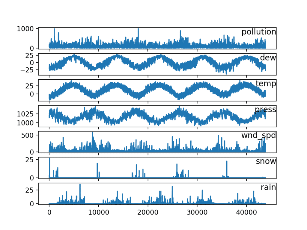
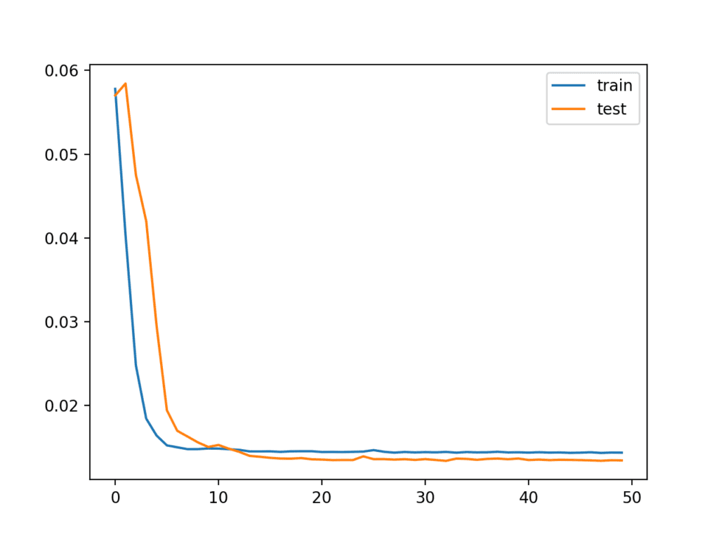
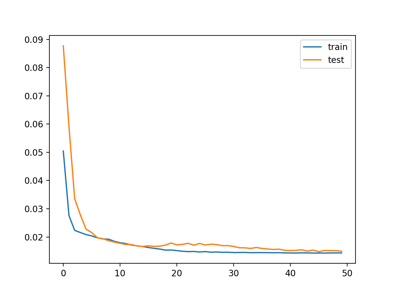


except wind *dir*, which is categorical.
Thanks, fixed!
how to use grid search for neurons
I want to apply grid search in this to tune neurons and add layers
and to find best parameters
See this post:
https://machinelearningmastery.com/tune-lstm-hyperparameters-keras-time-series-forecasting/
hello Jason,
I have run the code in my spyder and I know the RMSE index is good enough for this model. However, I added the accuracy index in this code, that is
model.compile(loss=’mae’, optimizer=’adam’, metrics=[‘accuracy’])
and the accuracy is totally the same in each epoch and is very low (0.0761). I also use my own data to run your code, and the result is the same, with good RMSE values but bad accuracy. I have troubled by this for several days and looking forward to your reply.
You cannot measure accuracy for regression.
Learn more here:
https://machinelearningmastery.com/classification-versus-regression-in-machine-learning/
Hi,Jason.
I have the same problem as qing.I don‘t know why we cannot measure accuracy for regression.And the website you provided cannot be opened.
Could you please help me with that?
Accuracy summarizes correct predictions for class labels. It cannot be used for regression. Instead you must calculate an error metric, like RMSE.
Learn more here:
https://machinelearningmastery.com/faq/single-faq/what-is-the-difference-between-classification-and-regression
And here:
https://machinelearningmastery.com/classification-versus-regression-in-machine-learning/
Thank you very much!
You’re welcome.
That is correct! You can only use accuracy for class labels. You could calculate RMSE or R^2 instead
hi,Jason,I‘m a new learner. There is no real curve and predicted curve in your tutorial.
I want to know how can I get it? I mean how to write it in the code?
Sorry, I don’t understand your question Mike, can you elaborate?
I guess he means the predicted value vs ground truth chart.
I see.
You can call model.predict() to get yhat and create a line plot with y and yhat.
I have done this in some other tutorials, for example:
https://machinelearningmastery.com/time-series-forecasting-long-short-term-memory-network-python/
If this is a challenge for you, I would suggest this tutorial is too advanced for you and I would encourage you to start with intro to time series here:
https://machinelearningmastery.com/start-here/#timeseries
How can predict next three months data for all the daily intervals here excluding weekends. Please help?
Hi Prakash…
To predict the next three months’ data for all daily intervals excluding weekends using multivariate time series forecasting with LSTMs in Keras, you can follow these steps:
—
### 1. **Understand the Data**
– Ensure your dataset has **features (independent variables)** and a **target variable** to predict.
– Ensure the dataset has time indices and does not include weekends for both training and predictions.
—
### 2. **Prepare the Dataset**
1. **Filter Out Weekends:**
– Use the
pandaslibrary to filter out rows with weekend dates.pythonimport pandas as pd
# Assume 'date' is your timestamp column
df['date'] = pd.to_datetime(df['date'])
df = df[~df['date'].dt.weekday.isin([5, 6])] # Exclude Saturdays and Sundays
2. **Scale Features:**
– Normalize or standardize the features for better LSTM performance.
pythonfrom sklearn.preprocessing import MinMaxScaler
scaler = MinMaxScaler()
scaled_data = scaler.fit_transform(df.drop(['date'], axis=1))
3. **Create Input Sequences:**
– LSTMs require sequential data. Create sequences for a rolling window.
pythondef create_sequences(data, seq_length):
X, y = [], []
for i in range(len(data) - seq_length):
X.append(data[i:i+seq_length, :-1]) # All features except the target
y.append(data[i+seq_length, -1]) # The target variable
return np.array(X), np.array(y)
seq_length = 30 # Example: Use 30 past days to predict the next day
X, y = create_sequences(scaled_data, seq_length)
—
### 3. **Build the LSTM Model**
pythonfrom keras.models import Sequential
from keras.layers import LSTM, Dense
model = Sequential([
LSTM(128, return_sequences=True, input_shape=(X.shape[1], X.shape[2])),
LSTM(64),
Dense(32, activation='relu'),
Dense(1) # Predicting one value
])
model.compile(optimizer='adam', loss='mse')
—
### 4. **Train the Model**
python
history = model.fit(X, y, epochs=50, batch_size=32, validation_split=0.2, shuffle=False)
—
### 5. **Make Predictions for the Next Three Months**
1. **Prepare Future Input Data:**
– Start with the last known data points and iterate to predict the next day, using each prediction as input for subsequent predictions.
pythonimport numpy as np
def forecast_future(model, initial_input, days_to_forecast):
input_seq = initial_input.copy()
predictions = []
for _ in range(days_to_forecast):
pred = model.predict(input_seq[np.newaxis, :, :])[0, 0]
predictions.append(pred)
# Update the input sequence with the new prediction
input_seq = np.vstack([input_seq[1:], np.append(input_seq[-1, :-1], pred)])
return predictions
2. **Generate Future Dates Excluding Weekends:**
– Calculate future dates without weekends.
pythonfrom datetime import timedelta
last_date = df['date'].max()
future_dates = []
while len(future_dates) < days_to_forecast: last_date += timedelta(days=1) if last_date.weekday() not in [5, 6]: # Skip weekends future_dates.append(last_date)
3. **Generate Predictions:**
- Use the
forecast_futurefunction to predict daily intervals and map them to future dates.pythonlast_input = scaled_data[-seq_length:, :] # Use the last known input sequence
predictions = forecast_future(model, last_input, len(future_dates))
# Inverse scale predictions
predictions = scaler.inverse_transform(np.array(predictions).reshape(-1, 1))
4. **Map Predictions to Dates:**
python
prediction_df = pd.DataFrame({
'date': future_dates,
'predicted_value': predictions.flatten()
})
---
### 6. **Validate the Model**
- Use a separate validation dataset to check the accuracy of your model.
- Consider tuning hyperparameters or using advanced architectures like Seq2Seq or attention mechanisms if accuracy is unsatisfactory.
---
### 7. **Plot the Results**
pythonimport matplotlib.pyplot as plt
plt.figure(figsize=(12, 6))
plt.plot(df['date'], df['target_variable'], label='Historical Data')
plt.plot(prediction_df['date'], prediction_df['predicted_value'], label='Forecast')
plt.legend()
plt.show()
---
This method ensures that predictions align with your requirements, excluding weekends and providing forecasts for the next three months.
Hi Jason, in all this implementation, how does thw feedback implementation occur? How do we account for lags in predicted time series?
Lags are accounted for as input time steps to the model.
Perhaps read this:
https://machinelearningmastery.com/faq/single-faq/what-is-the-difference-between-samples-timesteps-and-features-for-lstm-input
Many thanks for this incredibly useful example!
I think I might have a small suggestion: I’ve downloaded the “pollution” data set from the Github link provided, and I found out that maybe the column to be encoded is now column 8 and not 4 like in the original code, so I made this amendment and it all worked: (apologies if I’m missing something):
# I’ve replaced this line:
#values[:,4] = encoder.fit_transform(values[:,4])
# … with this line:
values[:,8] = encoder.fit_transform(values[:,8])
Thanks for your help!
Perhaps you downloaded the wrong dataset?
Here it is:
https://raw.githubusercontent.com/jbrownlee/Datasets/master/pollution.csv
good afternoon,i m new to machine learning and trying to run ur code on google colabs,but i getting the following error.
2003
2004 if not is_integer(x):
-> 2005 x = names.index(x)
2006
2007 self._reader.set_noconvert(x)
ValueError: ‘year’ is not in list
pls help me to slove out
Sorry, I don’t know about colab.
Try running the example on your workstation.
Hi Jason. Do you know why i can’t inverse scaler transform in inv_yhat and why appear this error?
operands could not be broadcast together with shapes (157,13) (7,) (157,13)
Perhaps this will help:
https://machinelearningmastery.com/machine-learning-data-transforms-for-time-series-forecasting/
I know how I can help you! In Jason’s code it is as follows:
inv_yhat = concatenate((yhat, test_X[:, -7:]), axis=1)
But make sure instead of 7 you use number_of_features -1, otherwise you have the value error.
So in my case, I use 31 features (including the one I wanna predict), and it is the following code:
inv_yhat = concatenate((yhat, test_X[:, -30:]), axis=1)
as well as for inv_y:
inv_y = concatenate((test_y, test_X[:, -30:]), axis=1)
Hope this helps!
Great post Jason. Thank you so much for making this material available for the community..
Thanks Francois, I’m glad it helped!
hi, jason. There were some problems under my environment which were keras2.0.4and tensorflow-GPU0.12.0rc0.
And Bug was that “TypeError: Expected int32, got list containing Tensors of type ‘_Message’ instead.”
The sentence that “model.add(LSTM(50, input_shape=(train_X.shape[1], train_X.shape[2])))” was located.
Could you please help me with that?
Regards,
yao
I would recommend this tutorial for setting up your environment:
https://machinelearningmastery.com/setup-python-environment-machine-learning-deep-learning-anaconda/
Thx a lot, doctor, it works! fabulous! 🙂
I’m glad to hear that.
Dr.Jason, I update TensorFlow then it works!
Sorry to bother you.
Thank you very much !
Best wishes !
I’m glad to hear that!
I met the same problem .
Did you uninstall all the programs previously installed or just set up the environment again?
Thx a lot!
Hi Jason,I set up my environment as the your tutorial.
scipy: 0.19.0
numoy: 1.12.1
matplotlib: 2.0.2
pandas: 0.20.1
statsmodels: 0.8.0
sklearn: 0.18.1
theano: 0.9.0.dev-c697eeab84e5b8a74908da654b66ec9eca4f1291
tensorflow: 0.12.1
Using TensorFlow backend.
keras: 2.0.5
But the bug still existed.Is the version of tensorFlow too odd?How could I do?
Thanks!
It might be, I am running v1.2.1.
Perhaps try running Keras off Theano instead (e.g. change the backend in the ~/.keras.jason config)
It seems that inv_y = scaler.inverse_transform(test_X)[:,0] is not the actual, should inv_yhat be compared with test_y but not pollution(t-1)? Because I think this inv_y here means pollution(t-1). Is this prediction equals to only making a time shifting from the current known pollution value (which means the models just take pollution(t) as the prediction of pollution(t+1))?
Sorry, I’m not sure I follow. Can you please restate your question, perhaps with an example?
Sorry for the confusing expression. In fact, the series_to_supervised() function would create a DataFrame whose columns are: [ var1(t-1), var2(t-1), …, var1(t) ] where ‘var1’ represents ‘pollution’, therefore, the first dimension in test_X (that is, test_X[:,0]) would be ‘pollution(t-1)’. However, in the code you calculate the rmse between inv_yhat and test_X[:,0], even though the rmse is low, it could only shows that the model’s prediction for t+1 is close to what it has known at t.
I am asking this question because I’ve ran through the codes and saw the models prediction pollution(t+1) looks just like pollution(t). I’ve also tried to use t-1, t-2 and so on for training, but still changed nothing.
Do you think the model tends to learn to just take the pollution value at current moment as the prediction for the next moment?
thanks 🙂
If we predict t for t+1 that is called persistence, and we show in the tutorial that the LSTM does a lot better than persistence.
Perhaps I don’t understand your question? Can you give me an example of what you are asking?
Hmm, it’s difficult to explain without a graph.
In a word, and also it’s an example, I want to ask two questions:
1. In the “make a prediction” part of your codes, why it computes rmse between predicted t+1 and real t, but not between predicted t+1 and real t+1?
2. After the “make a prediction” part of your codes run, it turns out that rmse between predicted t+1 and real t is small, is it an evidence that LSTM is making persistence?
RMSE is calculated for y and yhat for the same time periods (well, that was the intent), why do you think they are not?
Is there a bug?
I think Songbin Xu is right. By executing the statement at line 90: inv_y = inv_y[:,0], you compare the inv_yhat with inv_y. inv_y is the polution(t-1) and inv_yhat is the predicted polution(t).
On line 50 the second parameter the function series_to_supervised can be changed to 3 or 5, so more days of history are used. If you do so, an error occurs in the scaler.inverse_transform (line 89).
No worries, great tutorial and I learned a lot so far!
I see now, you guys are 100% correct. Thank you!
I have updated the calculation of RMSE and the final score reported in the post.
Note, I ran a ton of experiments on AWS with many different lag values > 1 and none achieved better results than a simple lag=1 model (e.g. an LSTM model with no BPTT). I see this as a bad sign for the use of LSTMs for autoregression problems.
Hi Dr. Jason,
As for this:
Updated Aug/2017: Fixed a bug where yhat was compared to obs at the previous time step when calculating the final RMSE. Thanks, Songbin Xu and David Righart.
It seems to have some errors on calculating RMSE based on (t-1) vs (t) different time slots before. I’m just curious how it is corrected? Can you elaborate that little bit more? Because for me, I’m still thinking it is RMSE based on (t-1) vs (t)
Thanks
I have updated tutorials that I think have better code and are easier to follow, you can get started here:
https://machinelearningmastery.com/start-here/#deep_learning_time_series
hey,Janson.The RMSE before you updated it was 3.386. Is this article RMSE 26.496 the correct answer after you updated it? In other words,inv_y = scaler.inverse_transform(test_X)[:,0] is not true,test_y = test_y.reshape((len(test_y), 1))
inv_y = concatenate((test_y, test_X[:, 1:]), axis=1)
inv_y = scaler.inverse_transform(inv_y) is the correct code,is it right?I find so many people use the incorrect code .
I don’t recall.
I recommend starting with a more recent tutorial using modern methods:
https://machinelearningmastery.com/start-here/#deep_learning_time_series
Hi Jason, great post!
Is it necessary remove seasonality (by seasonal differentiation) when we are using LSTM?
No, but results are often better.
Good article, thank.
Two questions:
What changes will be required if your data is sporadic? Meaning sometimes it could be 5 hours without the report.
And how do you add more timesteps into your model? Obviously you have to reshape it properly but you also have to calculate it properly.
You could fill in the missing data by imputing or ignore the gaps using masking.
What do you mean by “add more timesteps”?
But what should I do if all data is stochastic time sequence?
For example predicting time till the next event – when events frequency is stochastically distributed on the timeline.
Good question, this sounds like survival analysis to me, perhaps see if it applies:
https://en.wikipedia.org/wiki/Survival_analysis
Dr.Jason,
Thank you for an awesome post.
(I was practicing on load forecast using MLP and SVR (You also suggested on a comment in your other LSTM tutorials). I also tried with LSTM and it did almost perform like SVR. However, in LSTM, I did not consider time lags because I have predicted future predictor variables that I was feeding as test set. I will try this method with time lags to cross validate the models)
Nice Jack, let me know how you go.
Hi Jason,
Can I use ‘look back'(Using t-2 , t-1 steps data to predict t step air pollution) in this case?
If it’s available,that my input data shape will be [samples , look back , features] isn’t it?
You can Adam, see the series_to_supervised() function and its usage in the tutorial.
Hi Jason,
If I used n_in=5 in series_to_supervised() function,in your tutorial the input shape will be [samples, 1 , features*5].Can I reshape it to [samples, 5 , features]?If I can, what is the difference between these two shape?
The second dimension is time steps (e.g. BPTT) and the third dimension are the features (e.g. observations at each time step). You can use features as time steps, but it would not really make sense and I expect performance to be poor.
Here’s how to build a model multiple time steps for multiple features:
And that’s it. I just tested and it looks good. The RMSE calculation will blow up, but you guys can fix that up I figure.
Jason, great post, very clear, and very useful!! I’m about 90% with you and think a few folks may be stuck on this final point if they try to implement multi-feature, multi-hour-lookback LSTM.
Seems like by making adjustments above, I’m able to make a prediction, but the scaling inversion doesn’t want to cooperate. The reshape step now that we have multiple features and multiple timesteps has a mismatch in the shape, and even if I make the shape work, the concatenation and inversion still don’t work. Could you share what else you changed in this section to make it work? I’m not so concerned about the RMSE as much as that I can extract useful predictions. Thank you for any insight since you’ve been able to do it successfully.
# make a prediction
yhat = model.predict(test_X)
test_X = test_X.reshape((test_X.shape[0], test_X.shape[2]))
# invert scaling for forecast
inv_yhat = concatenate((yhat, test_X[:, 1:]), axis=1)
inv_yhat = scaler.inverse_transform(inv_yhat)
inv_yhat = inv_yhat[:,0]
…
Hi Jason,
Great and useful article.
I am somewhat puzzled by the number of features you specify to forecast the pollution rate based on data from the previous 24 hours.
Do not we have 8 features for each time-step and not 7?
After generating data to supervise with the function series_to_supervised(scaled,24, 1), the resulting array has a shape of (43800, 200) which is 25 * 8.
To invert the scaling for forecast I made few modifications. I used scaled.shape[1] below but in my opinion it could be n_features. Moreover, I don’t know if the values concatenated to yhat and test_y really matter, as long as they have been scaled with fit_transform and the array has the right shape.
yhat = model.predict(test_X)
test_X = test_X.reshape((test_X.shape[0], n_obs))
# invert scaling for forecast
inv_yhat = concatenate((yhat, test_X[:, 1:scaled.shape[1]]), axis=1)
inv_yhat = scaler.inverse_transform(inv_yhat)
inv_yhat = inv_yhat[:,0]
# invert scaling for actual
test_y = test_y.reshape((len(test_y), 1))
inv_y = concatenate((test_y, test_X[:, 1:scaled.shape[1]]), axis=1)
inv_y = scaler.inverse_transform(inv_y)
inv_y = inv_y[:,0]
The model has 4 layers with dropout.
After 200 epochs I have got
loss: 0.0169 – val_loss: 0.0162
And a rmse = 29.173
Regards.
We have 7 features because we drop one in section “2. Basic Data Preparation”.
Hi Jason,
It’s really weird to me :(, as I used your code to prepare the data (pollution.csv) and I have 9 fields in the resulting file.
[date, pollution, dew, temp, press, wnd_dir, wnd_spd, snow, rain]
😯
Date and wind direction are dropped during data preparation, perhaps you accidentally skipped a step or are reviewing a different file from the output file?
Hi Jason,
So that’s fine, in my case I have 8 features.
When reading the file, the field ‘date’ becomes the index of the dataframe and the field ‘wnd_dir’ is later label encoded, as you do above in “The complete example” lines 42-43.
It is now much clearer for me. I am not puzzled anymore. 😉
Thanks a lot for all the information contained in your articles and your e-books.
They are really very informative.
🙂
I’m glad to hear that!
Hi Jason,
I think the output is column var1(t), that means:
train_X, train_y = train[:, 0:n_obs], train[:, -(n_features+1)]
am I right?
In case the “pollution” is in the last column, it is easy to get train[:, -1]
am i right?
I just want to verify that I understand your post.
Thank you, Jason
I have some confusion for this problem.
I want to use a bigger windows (I want to go back in time more, for example t-5 to include more data to make a prediction of the time t) and use all of this to predict one variable (such as just the pollution), like you did. I think predicting one variable will be more accurate than predicting many. Such as pollution and temperature.
What should I do to apply more shift?
I show in another comment how to update the example to use lab obs as input.
I will update the post and add an example to make it clearer.
First of all, thanks for your work and the effort you put in!
I tried to implement your suggestion for increasing the timesteps (BPTT). I have intergrated your code but I keep getting this error in when reshaping test_X in the prediction step:
test_X = test_X.reshape((test_X.shape[0], test_X.shape[2]))
ValueError: cannot reshape array of size 490532 into shape (35038,7)
Do you have any tips on how to proceed?
I will update the post with a worked example. Adding to trello now…
Hi Jason.
In the code you wrote above, should the following code:
train_X = train_X.reshape((train_X.shape[0], n_hours, n_features))
be actually
train_X = train_X.reshape((train_X.shape[0]/n_hours, n_hours, n_features))
Why is that?
Hi,Janson.I am a new leaner. First, thank fou for your share! But, when I run the complete code, it has an error: pyplot.plot(history.history[‘val_loss’], label=’test’)
KeyError: ‘val_loss’
How can I sovle it!
Perhaps you did not use a validation dataset when fitting the model. In that case you cannot plot validation loss.
Hi Jason,
Thank you for this excellent tutorial. I recently started working on LSTM methods. I have a doubt regarding this input shape. In case if the n_hour >1 , how to inverse transform the scaled values? Thanks in advance. Thanks in advance.
You’re welcome.
This will help with the input shape:
https://machinelearningmastery.com/faq/single-faq/what-is-the-difference-between-samples-timesteps-and-features-for-lstm-input
Hi Jason, I get the following error from line # 82 of your ‘Complete Example’ code.
ValueError: Error when checking : expected lstm_1_input to have 3 dimensions, but got array with shape (34895, 8)
I think LSTM() is looking for (sequences, timesteps, dimensions). In your code, line # 70, I believe 50 is timesteps while input_shape (1,8) represents the dimensions. May be it’s missing ‘sequences’ ?
Appreciate your response.
Ensure that you first prepare the data (e.g. convert “raw.csv” to “pollution.csv”).
I have the same error too. Cannot figure out what’s wrong
Something changed, the problem is on the model evaluation section, specifically the reshape line
test_X = test_X.reshape((test_X.shape[0], test_X.shape[2]))
as it is, is 2 dimensions (34895, 8)
we need to add one dimension but I can’t figure out how (noob here)
tried this: test_X = test_X.reshape((test_X.shape[0], test_X.shape[2]))
but didn’t work (IndexError: tuple index out of range)
any ideas anyone?
You can use the reshape() function or the expand_dimensions() function in NumPy.
https://docs.scipy.org/doc/numpy/
Does that help?
Greetings Sir..
I’ve run into the same problem as well. And I’m confident that I’m using “pollution.csv” data.. How can I rectify this?
I have some suggestions here:
https://machinelearningmastery.com/faq/single-faq/why-does-the-code-in-the-tutorial-not-work-for-me
Hi Jason, I am wondering what the issue that I’m getting is caused by, maybe a different type of dataset then the example one. basically when I run the history into the model, When i check the History.history.keys() I only get back ‘loss’ as my only key.
You must specify the metrics to collect when you compile the model.
For example, in classification:
Hi Jason,
If you replace in this example the target by a binary target, let us say one that says if the var_1 goes up or not in the next move, thus : :
reframed[‘var1(t)_diff’]=reframed[‘var1(t)’].diff(1)
reframed[‘target_diff’]=reframed[‘var1(t)_diff’].apply(lambda x : (x>0)*1)
it gives this error :
””
You are passing a target array of shape (8760, 1) while using as loss
categorical_crossentropy.categorical_crossentropyexpects targets to be binary matrices (1s and 0s) of shape (samples, classes). If your targets are integer classes, you can convert them to the expected format via:””’
I have :
test_y.shape as (35038,)
but if we follow another example from you with the PIMA dataset on a simple classification : https://machinelearningmastery.com/tutorial-first-neural-network-python-keras/
which was :
X = dataset[:,0:8]
Y = dataset[:,8]
model = Sequential()
model.add(Dense(12, input_dim=8, activation=’relu’))
model.add(Dense(8, activation=’relu’))
model.add(Dense(1, activation=’sigmoid’))
model.compile(loss=’binary_crossentropy’, optimizer=’adam’, metrics=[‘accuracy’])
model.fit(X, Y, epochs=150, batch_size=10)
it gives no error whereas the Y have the same shape … why ?
How can we make it work for the lstm classification please ?
Thanks
I have an example of LSTMs for time series classification here:
https://machinelearningmastery.com/how-to-develop-rnn-models-for-human-activity-recognition-time-series-classification/
Yes thanks I looked at it:
if you do one example inside :
trainX, trainy = load_dataset_group(‘train’, path + ‘HARDataset/’)
trainy = trainy – 1
Note :
set(list(pd.DataFrame(trainy)[0]))
Out[217]: {0, 1, 2, 3, 4, 5}
But
trainy_postcategorical = to_categorical(trainy)
trainy_postcat.shape
gives
print(trainy_postcat.shape)
(7352, 7)
which means one additional variable has been created while we were expecting 6 dummies only.
pd.DataFrame(trainy_postcat)[0].sum() gives 0 so empty column for 1st one
Come back to the sahpe of lstm.
the output of your pre process work gives :
trainy_postcat.shape
Out[219]: (7352, 7)
which for a single dummy (the case of this article and my original question)
is the analogy of
”’ You are passing a target array of shape (8760, 1) ”
which should be good.
Any idea ? the activity recognition analogy does not solve the shape issue.
Sorry, I don’t have the capacity to review/debug your code, more here:
https://machinelearningmastery.com/faq/single-faq/can-you-read-review-or-debug-my-code
Hello Jason,
Thank you for such a nice tutorial.
Since you have published a similar topic and few other related topics in one of your paid books (LSTM networks), should the reader also expect some different topics covered in it?
I’m an ardent fan of your blogs since it covers most of the learning material and therefore, it makes me wonder that will be different in your book?
Thanks Arman.
The book does not cover time series, instead it focuses on teaching you how to implement a suite of different LSTM architectures, as well as prepare data for your problems.
Some ideas were tested on the blog first, most are only in the book.
You can see the full table of contents here:
https://machinelearningmastery.com/lstms-with-python/
The book provides all the content in one place, code as well, more access to me, updates as I fix bugs and adapt to new APIs, and it is a great way to support my site so I can keep doing this.
Thank you for accepting my opinions, such a pleasure!
Running the codes u modified, still something puzzles me here,
1. Have u drawn the waveforms of inv_y and inv_yhat in the same plot? I think they looks quite like persistence.
2. Curiously, I computed the rmse between pollution(t) and pollution(t-1) in test_X, it’s 4.629, much lower than your final score 26.496, does it mean LSTM performs even worse than persistence?
3. I’ve tried to remove var1 at t-1, t-2, … , and I’ve also tried to use lag values>1, and also assign different weights to the inputs at different timesteps, but none of them improved, they performed even worse.
Do you have any other ideas to avoid the whole model to learn persistence?
Looking forward to your advices 🙂
Thank you for pointing out the fault!
The final line plot shows loss on the transformed train and test sets.
Yes, LSTMs are no good at autoregression, yet I keep getting asked to develop examples (tens of emails per day)… See here:
https://machinelearningmastery.com/suitability-long-short-term-memory-networks-time-series-forecasting/
Consider developing a baseline with an MLP, you’ll find it tough to beat it with an LSTM!
Why are you only training with a single timestep (or sequence length)? Shouldn’t you use more timesteps for better training/prediction? For instance in https://github.com/fchollet/keras/blob/master/examples/lstm_text_generation.py they use 40 (maxlen) timesteps
Yes, it is just an example to help you get started. I do recommend using multiple time steps in order to get the full BPTT.
Hi Jason and Varuna,
When the timesteps = 1 as you mentioned, does it mean the value of t-1 time was used to predict the value of t time? Is moving window a method to use multiple time steps? Is there any other way? Has Keras any functions of moving window?
Thank you very much.
Keras treats the “time steps” of a sequence as the window, kind of. It is the closest match I can think of.
Hi Jason,
I met some problem when learning your codes.
dataset = read_csv(‘D:\Geany\scriptslym\raw.csv’, parse_dates = [[‘year’, ‘month’, ‘day’, ‘hour’]],index_col=0, data_parser=parse)
Traceback (most recent call last):
File “”, line 1, in
dataset = read_csv(‘D:\Geany\scriptslym\raw.csv’, parse_dates = [[‘year’, ‘month’, ‘day’, ‘hour’]],index_col=0, data_parser=parse)
NameError: name ‘parse’ is not defined
>>>
It looks like you have specified a function “parse” but not defined it.
Hi Jason,
Can I use “keras.layers.normalization.BatchNormalization” as a substitute for “sklearn.preprocessing.MinMaxScaler”?
No, they do very different things.
Hi Jason, Its a very Informative article. Thanks. I have a question regarding forecasting in time series. You have used the training data with all the columns while learning after variable transformations and the same has been done for the test data too. The test data along with all the variables were used during prediction. For instance, If I want to predict the pollution for a future date, Should I know the other inputs like dew, pressure, wind dir etc on a future date which I’m not aware off? Another question is, Suppose we have same data about multiple regions(let us consider that the pollution among these regions is not negligible), How can we model so that the input argument while prediction is the region name along with time to forecast just for that one region.
It depends on how you define your model.
The model defined above uses the variables from the prior time step as inputs to predict the next pollution value.
In your case, maybe you want to build a separate model per region, perhaps a model that improves performance by combining models across regions. You must experiment to see what works best for your data.
Thanks! I missed the trick of converting the time-series to supervised learning problem. That alone is sufficient even for multiple regions I guess. We just have to submit the input parameters of the previous time stamp for the specific region during prediction. We may also try one-hot encoding on the region variable too during data preprocessing.
Thank you for your excellent blog, Jason. I’ve really learnt a lot from your nice work recently. After this post, I’ve already known how to transform data into data that formates LSTM and how to construct a LSTM model.
Like the question aksed by Naveen Koneti, I have the same puzzle.
Recently I’ve worked on some clinical data. The data is not like the one we used in this demo. It is consist of hunderds of patients, each patient has several vital sign records. If it is about one individual’s records through many years, I can process the data as what you told us. I wonder how I can conquer this kind of data. Could you give me some advice, or tell me where I can find any solutions about it?
If I didn’t state my question clearly and you’re interested it, pls let me know.
Thanks in advance.
PS. the data set in my situation is like this
[ID date feature1 feature2 feautre3 ]
[patient1 date1 value11 value12 value13 ]
[patient1 date2 value21 value22 value23 ]
[patient2 date1 value31 value32 value33 ]
[patient2 date2……………………………………..]
[patient3 ……………………………………………..]
You could model one patient at a time, or groups or all of them. Try different approaches and see what works best.
I cannot tell you what would work best – I have no idea – you must discover it.
See this post:
https://machinelearningmastery.com/a-data-driven-approach-to-machine-learning/
Hi Naveen, I have the same your question: the model is defined such that if you know the input features at time t, then you can predict the target value at time t+1. If you want to predict the target variable at time t+2, though, you would need to know the input features at time t+1. If a feature does not change over time, it is no problem; but if a feature changes over time, then its value at time t+1 is not known and may be different from its value at time t.
I am thinking that to solve this, you would need to define such features as output of the model as well as the target variable. In this way, at time t, you can predict the target variable for time t+1, but also the feature for time t+1, so that this predicted value can be used as input to predict the target variable for time t+2.
What do you think about that? Did you think of a different solution?
Many thanks
Hi,
again a nice post for the use of lstm’s!
I had the following idea when reading.
I would like to build a network, in which each feature has its own LSTM neuron/layer, so that the input is not fully connected.
My idea is adding a lstm layer for each feature and merge it with the merge layer and feed these results to the output neurons.
Is there a better way to do this? Or would you recommend to avoid this because the features are poorly abstracted? On the other hand, this might also be interesting.
Thank you!
Try it and see if it can out-perform a model that learns all features together.
Also, contrast to an MLP with a window – that often does better than LSTMs on autoregression problems.
Hi Jason,
I have two questions:
1) I have a question/ notice regarding the scaling of the Y variable (pollution). The way you implement the rescaling between [0-1] you consider the entire length of the array (all of the 43799 observations -after the dropna-).
Is it rightto rescale it that way? By doing so we are incorporating information of the furture (test set) to the past (train set) because the scaler is “exposed” to both of them and therefore we introduce bias.
If you agree with my point what could be a fix?
2) Also the activation function of the output (Y variable) is sigmoid, that’s why we rescale it within the [0,1] range. Am I correct?
Thanks for sharing the article!
No, ideally you would develop a scaling procedure on the training data and use it on test and when making predictions on new data.
I tried to keep the tutorial simple by scaling all data together.
The activation on the output layer is ‘linear’, the default. This must be the case because we are predicting a real-value.
Hi,
First I wanna thanks for your helpful and practical blog.
I tried to separate train and test set to do normalization on training but I have gotten error related to test set shape something like that “ValueError: cannot reshape array of size 136 into shape (34,2,4)”, which I don’t know how to fix it!
Do you have an example on LSTM which run normalization on train and used in test, or do you explain that in your book?
Thanks
This post will help you learn how to reshape your input data:
https://machinelearningmastery.com/reshape-input-data-long-short-term-memory-networks-keras/
Hi,
I did some changes and just use transform method on test set, is that correct?
firstly I divided my data-set to two different sets ,(train and test)
secondly I ran fit_transform on train set and transform on test set
But I get rmse=0 ? which seems weird. am I correct?
Sounds correct.
An RMSE of zero suggests a bug or a very simple modeling problem.
Thank you very much for your tutorial.
I have one question,
but I failed to read the NW in pollution. csv.(cbwd column)
values = values.astype(‘float32’)
ValueError: could not convert string to float: NW
How do you fix it?
sorry, I saw the text above and solved it.
Glad to hear it!
Hi, I would like to know how did you fix it? I still have that problem, tried to find the solution above but didn’t find one. Thank you !
You have to prepare the Data befor you convert (see “Basic Data Preparation”). In Jason’s complete Example of the LSTM this preparation step is missing (more likely left out).
Yes the note above the complete example says clearly:
Hi Jason!
I assume there is little mistake when you calculate RMSE on test data.
You must write this code before calculate RMSE:
inv_y = inv_y[:-1]
inv_yhat = inv_yhat[1:]
Thus, RMSE equals 10.6 (on the same data, in my case), that is much less than 26.5 in your case.
Sorry, I don’t understand your comment and snippet of code, can you spell out the bug you see?
This beats further exploration
I agree with @Dmitry here. The prediction “inv_yhat” is one index ahead of real output “inv_y”.
It can be seen by plotting predicted output v/s real output:
pyplot.plot(inv_y[:-1,], color=’green’, marker=’o’, label = ‘Real Screening Count’)
pyplot.plot(inv_yhat[1:,], color=’red’, marker=’o’, label = ‘Predicted Screening Count’)
pyplot.legend()
pyplot.show()
Compute RMSE by skipping first element of inv_yhat, and better RSME score is presented:
rmse = sqrt(mean_squared_error(inv_y[:-1,], inv_yhat[1:,]))
print(‘Test RMSE: %.3f’ % rmse)
rmse = sqrt(mean_squared_error(inv_y, inv_yhat))
print(‘Test RMSE: %.3f’ % rmse)
Hi Jason,
great post! I was waiting for meteo problems to infiltrate the machinelearningmastery world.
Could you write something about the changed scenareo where, given the weather conditions and pollution for some time, we can predict the pollution for another time or place with given weather conditions?
For example: We have the weather conditions and pollution given for Beijing in 2016, and we have the weather conditions given for Chengde (city close to Bejing) also in 2016. Now we want to know how was the pollution in Chengde in 2016.
Would be great to learn about that!
Great suggestion, I like it. An approach would be to train the model to generalize across geographical domains based only on weather conditions.
I have tried not to use too many weather examples – I came from 6 years of work in severe weather, it’s too close to home 🙂
Hi Jason,
I have read many of your posts about LSTM. I have not completely clear the difference between the parameters batch_size and time_steps. Batch_size means when the memory is reset (right?), but this shouldn’t have the same value of time_steps that, if I have understood correctly, means how often the system makes a prediction?
Great question!
Batch size is the number of samples (e.g. sequences) to that are used to estimate the gradient before the weights are updated. The internal state is reset at the end of each batch after the weights are updated.
One sample is comprised of 1 or more time steps that are stepped over during backpropagation through time. Each time step may have one or more features (e.g. observations recorded at that time).
Time steps and batch size and generally not related.
You can split up a sequence to have one-time step per sequence. In that case you will not get the benefit of learning across time (e.g. bptt), but you can reset state at the end of the time steps for one sequence. This an odd config though and really only good to showing off the LSTMs memory capability.
Does that help?
Thanks, now it’s more clear!
Hi,I ger this error at this step, could you help me please?
model.add(LSTM(50, input_shape=(train_X.shape[1], train_X.shape[2])))
—————————————————————————
TypeError Traceback (most recent call last)
in ()
—-> 1 model.add(LSTM(50, input_shape=(train_X.shape[1], train_X.shape[2])))
C:\Anaconda3\lib\site-packages\keras\models.py in add(self, layer)
431 # and create the node connecting the current layer
432 # to the input layer we just created.
–> 433 layer(x)
434
435 if len(layer.inbound_nodes) != 1:
C:\Anaconda3\lib\site-packages\keras\layers\recurrent.py in __call__(self, inputs, initial_state, **kwargs)
241 # modify the input spec to include the state.
242 if initial_state is None:
–> 243 return super(Recurrent, self).__call__(inputs, **kwargs)
244
245 if not isinstance(initial_state, (list, tuple)):
C:\Anaconda3\lib\site-packages\keras\engine\topology.py in __call__(self, inputs, **kwargs)
556 ‘
layer.build(batch_input_shape)‘)557 if len(input_shapes) == 1:
–> 558 self.build(input_shapes[0])
559 else:
560 self.build(input_shapes)
C:\Anaconda3\lib\site-packages\keras\layers\recurrent.py in build(self, input_shape)
1010 initializer=bias_initializer,
1011 regularizer=self.bias_regularizer,
-> 1012 constraint=self.bias_constraint)
1013 else:
1014 self.bias = None
C:\Anaconda3\lib\site-packages\keras\legacy\interfaces.py in wrapper(*args, **kwargs)
86 warnings.warn(‘Update your
' + object_name +call to the Keras 2 API: ‘ + signature, stacklevel=2)87 '
—> 88 return func(*args, **kwargs)
89 wrapper._legacy_support_signature = inspect.getargspec(func)
90 return wrapper
C:\Anaconda3\lib\site-packages\keras\engine\topology.py in add_weight(self, name, shape, dtype, initializer, regularizer, trainable, constraint)
389 if dtype is None:
390 dtype = K.floatx()
–> 391 weight = K.variable(initializer(shape), dtype=dtype, name=name)
392 if regularizer is not None:
393 self.add_loss(regularizer(weight))
C:\Anaconda3\lib\site-packages\keras\layers\recurrent.py in bias_initializer(shape, *args, **kwargs)
1002 self.bias_initializer((self.units,), *args, **kwargs),
1003 initializers.Ones()((self.units,), *args, **kwargs),
-> 1004 self.bias_initializer((self.units * 2,), *args, **kwargs),
1005 ])
1006 else:
C:\Anaconda3\lib\site-packages\keras\backend\tensorflow_backend.py in concatenate(tensors, axis)
1679 return tf.sparse_concat(axis, tensors)
1680 else:
-> 1681 return tf.concat([to_dense(x) for x in tensors], axis)
1682
1683
C:\Anaconda3\lib\site-packages\tensorflow\python\ops\array_ops.py in concat(concat_dim, values, name)
998 ops.convert_to_tensor(concat_dim,
999 name=”concat_dim”,
-> 1000 dtype=dtypes.int32).get_shape(
1001 ).assert_is_compatible_with(tensor_shape.scalar())
1002 return identity(values[0], name=scope)
C:\Anaconda3\lib\site-packages\tensorflow\python\framework\ops.py in convert_to_tensor(value, dtype, name, as_ref, preferred_dtype)
667
668 if ret is None:
–> 669 ret = conversion_func(value, dtype=dtype, name=name, as_ref=as_ref)
670
671 if ret is NotImplemented:
C:\Anaconda3\lib\site-packages\tensorflow\python\framework\constant_op.py in _constant_tensor_conversion_function(v, dtype, name, as_ref)
174 as_ref=False):
175 _ = as_ref
–> 176 return constant(v, dtype=dtype, name=name)
177
178
C:\Anaconda3\lib\site-packages\tensorflow\python\framework\constant_op.py in constant(value, dtype, shape, name, verify_shape)
163 tensor_value = attr_value_pb2.AttrValue()
164 tensor_value.tensor.CopyFrom(
–> 165 tensor_util.make_tensor_proto(value, dtype=dtype, shape=shape, verify_shape=verify_shape))
166 dtype_value = attr_value_pb2.AttrValue(type=tensor_value.tensor.dtype)
167 const_tensor = g.create_op(
C:\Anaconda3\lib\site-packages\tensorflow\python\framework\tensor_util.py in make_tensor_proto(values, dtype, shape, verify_shape)
365 nparray = np.empty(shape, dtype=np_dt)
366 else:
–> 367 _AssertCompatible(values, dtype)
368 nparray = np.array(values, dtype=np_dt)
369 # check to them.
C:\Anaconda3\lib\site-packages\tensorflow\python\framework\tensor_util.py in _AssertCompatible(values, dtype)
300 else:
301 raise TypeError(“Expected %s, got %s of type ‘%s’ instead.” %
–> 302 (dtype.name, repr(mismatch), type(mismatch).__name__))
303
304
TypeError: Expected int32, got list containing Tensors of type ‘_Message’ instead.
Perhaps check that your environment is setup correctly:
https://machinelearningmastery.com/setup-python-environment-machine-learning-deep-learning-anaconda/
Also, ensure that you have copied all of the code.
Hi Jason,
I was curious if you can point me in the right direction for converting data back to the actual values instead of scaled.
Yes, you can invert the scaling.
This tutorial demonstrates how to do that Neal.
Hi Jason, I did have an issue converting back to actual values, but was able to get past it using the drop columns on the reframed data which got me past it.
When looking at my predicted values vs actual values, I’m noticing that my first column has a prediction and a true value, but for every other variable, I only see what I can assume is a prediction? does this make a prediction on every column, or just one particular one.
Im sorry for asking a question such as this, I just think I’m confusing myself looking at my results.
The code in the tutorial only predicts pollution.
Dr. Jason,
I have been trying with my own dataset and I am getting an error “ValueError: operands could not be broadcast together with shapes (168,39) (41,) (168,39)” when I try to do
inv_yhat = scaler.inverse_transform(inv_yhat)as you have in line 86 in your script. I still can not figure out where my issue is. I haveyhat.shapeas (168,1) and test_X.shapeas (168,38). When I do this,inv_yhat = np.concatenate((yhat, test_X[:, 1:]), axis=1), myinv_yhat.shapeis (168,39). I still can not figure whyinverse_transformgives that error.The shape of the data must be the same when inverting the scale as when it was originally scaled.
This means, if you scaled with the entire test dataset (all columns), then you need to tack the yhat onto the test dataset for the inverse. We jump through these exact hoops at the end of the example when calculating RMSE.
This seems to be the same issue I am having at the moment also. i concatenate my inv_yhat with my test_X like you said, but the shape of inv_yhat after is still not taking into account the 2nd numbers(in posts case (41,).
Ask a question in stackoverflow and post the link, I should be able to help. I spent lots of time on this and have a decent idea now.
Yes, you’re right! I did that and it worked, nice! Thank you for your comment!
Glad to hear that Jack.
How did you solve the problem??
here’s link to solution on stackoverflow:
https://datascience.stackexchange.com/questions/22488/value-error-operands-could-not-be-broadcast-together-with-shapes-lstm
Nice!
I am having the same problem, but cannot solve the issue. everytime i try to concatenante them together, there is not change to my inv_yhat variable. i still am unable to understand this issue if you can expand a bit more that would be amazing
@John Regilina,
Check the shape of data after you scale the data and then check the scale again after you do the concatenation. Remember, when your
yhatshape will be (rowlength,1) and after concatenationinv_yhatshould be the same shape after you scaled the data. Look at Dr.Jason’s answer to my comment/question. Hope that will help. (Thanks to Dr.Jason saved a lot of my time)Hello Sir, thank you for the awesome tutorial. But I still couldn’t understand what exactly needs to be done. I am getting the error:
> operands could not be broadcast together with shapes (12852,27) (14,) (12852,27) ”
This the line which generates the error:
inv_yhat = scaler.inverse_transform(inv_yhat).fit()
Could you please give me a small example to understand what went wrong. Thanks in advance Sir.
I am also stuck with same thing. How did you fix it?
Same question here, how did everyone fix this? From your answers I cannot deduce what exactly went wrong in your case, and what you did to solve it.
I am suffering from the same problem when i am trying it on my dataset having np.shape(test_X) as (89070,13) size. Kindly kindly help me out if you have got the solution.
This will help with preparing data for LSTMs:
https://machinelearningmastery.com/faq/single-faq/what-is-the-difference-between-samples-timesteps-and-features-for-lstm-input
Hi Jason, In dataset.drop(‘No’, axis =1, inplace = True), what is the purpose of ‘axis’ and ‘inplace’?
Great question.
We specify to remove the column with axis=1 and to do it on the array in memory with inplace rather than return a copy of the array with the column removed.
Fabulous tutorials Jason!
Thanks Lizzie.
Can you show how the multi variate forecast looks like?
Looks like you missed it in the article.
Sure,
You can plot all predictions as follows:
You get:
It’s a mess, you can plot the last 100 time steps as follows:
You get:
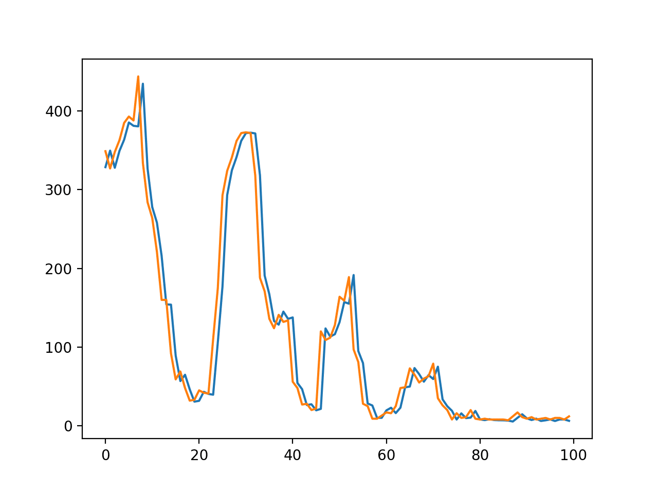
The predictions look like persistence.
Jason, what am I missing, looking at your plot of the most recent 100 time steps, it looks like the predicted value is always 1 time period after the actual? If on step 90 the actual is 17, but the predicted value shows 17 for step 91, we are one time period off, that is if we shifted the predicted values back a day, it would overlap with the actual which doesn’t really buy us much since the next hour prediction seems to really align with the prior actual. Am I missing something looking at this chart?
This is what a persistence forecast looks like, that value(t) = value(t-1).
So how would you get the true predicted value(t)? I am thinking of the last record in the time series where we are trying to predict the value for the next hour.
Sorry, I don’t follow. Perhaps you can restate your question?
Hello Jason Brownlee
Thank you for your great posts. I run the model above for my data and it works perfectly, how ever when I draw the real data (blue one – inv_y) and the prediction (the orange one – inv_yhat), the result shows the prediction is delay after 1 step. it should be predicted one step before as your graph. your model is the same with the matlab tool:
https://nl.mathworks.com/videos/maglev-modeling-with-neural-time-series-tool-68797.html
And after running the model, I applyed realtime this model for my problem to compute the inv_yhat in every step. I got the result is really bad, since I have never had the real inv_y. I took the prediction to feed the input ( instead of real data inv_y)
My problem is: I received some signals as inputs, then I labeled offline to have output (real data inv_y or the first column in train_X)
Do you have the model that trains without the real data in the first column?????? thank you
Your model may have low skill and be simply predicting the input as the output (e.g. persistence).
You may need to continue to develop your model, I list some ideas for lifting model skill here:
https://machinelearningmastery.com/improve-deep-learning-performance/
hi, i have the same confusion as you. i think the prediction problem should be value_predict(t-1) = value_real(t). the label “train_y” indicates value_real(t+1). we input the train_x(t) into the model to get the prediction and the prediction should match “train_y” , not one step after “train_y”. did you solve this problem?
It’s definitely similar to a persistence model since we trained the model using the
var1(t-1)feature (i.e. the lagged pollution feature). The model certainly found that to be the strongest predictor. This would be ok if we were doing predictions later on an hour-by-hour basis. But, if, say we want to predict the pollution 20 hours from now, we aren’t yet going to know what the hour-19 pollution is. So it seems like cheating to include this variable in the training and prediction sets.I removed this variable to train the model, leaving other parameters about the same, and was then only able to get a minimum validation loss of 0.55 and test RMSE of 87.02
Nice work.
It’s not cheating, it comes down to different framings of the problem based on the requirements of the problem.
This post can help if you want to explore direct multi-step forecasting:
https://machinelearningmastery.com/multi-step-time-series-forecasting-long-short-term-memory-networks-python/
It looks the prediction is pretty good. Can we say the lstm model is good?
I think LSTMs are poor at autoregression.
Hi, Jason.I have a question on the transform, which is I found the predicted data after inverse_transform() were not same as the original value. For example, my original data is at the range from 0 to 850, but the prediction data is at 0 to 8. Is there any problem?
Perhaps there is a bug in your implementation?
Hi Jason
I have two questions:
(a) based on the graphs that you have shown for the y_inv and yhat_inv, it looks like your model has overfit on the test set. Don’t you agree ?
(b) In all time series prediction posts I have seen, the validation part uses the tail of the data to do validation (predict(yhat)). How can we modify the code in order to predict the future which is not covered in the dataset.
The model in this tutorial is probably underfit – e.g. it learned a persistence model.
Fit the data on all available data then call model.predict() to predict out of sample.
Wind dir is label encoded not wind speed!!!
Yes.
First of all, thanks. All of this material on the blog is super interesting, and helpful and making me learn a lot.
Of course… I have a question.
I’m surprised by the use of LSTMs here. The property of them being “stateful” I guess is being used. But is there “sequence” information flowing?
So when I used LSTMs in Keras for text classification tasks (sentence, outcome), each “sentence” is a sequence. Each observation is a sequence. It’s an ordered array of the words in the sentence (and it’s outcome).
In this example, I could not see a sense in which var1(t-1) is linked to var1(t-2). Aren’t they being treated as independent Xs in a regression problem? (predicting var8(t))
Correct, we are not providing a sequence of observations and therefore not getting good BPTT.
Based on my tests, I have found LSTMs to be poor at autoregression, and in this case, as I added more history to the model (longer sequences), performance degraded.
I would strongly encourage you to use an MLP baseline that any MLP would have to out-perform.
See this post for more on the limitations of LSTM for time series:
https://machinelearningmastery.com/suitability-long-short-term-memory-networks-time-series-forecasting/
Awesome article, as always.
Btw, what is your view on using an autoencoder/ restricted Boltzmann layer compressing features/ features before feeding an LSTM network ? For example, if one has a financial timeseries to forecast, e.g. a classifier trying to predict increase or decrease in a look ahead time window, via numerous technical indicators and/or other candidate exogenous leading indicators…..
Could you write an article based on that idea?
I have seen better results from large MLPs, nevertheless, try it and see how you go.
autoencoder/ restricted Boltzmann layers also deal with multicollinearity issues… do MLPs also deal with multicollinearity if you have multicollinearity in the features, right?
MLPs are more robust to multicollinearity than linear models.
Hi, I am always amazed at your article. Thank you.
I have a question.
Is this LSTM code now weighted for each features?
Nowdays, I’m predicting precipitation, that is the trend is correct, but the amount is not right.
What’s wrong with that?:(
Thanks!
Sorry, I’m not sure I understand the question, perhaps you could rephrase it?
I can say that I would expect better skill if the data was further prepared – e.g. made stationary.
Hi Jason,
Thanks for wonderful explanation!
Could you please help me to understand dimensionality reduction concept. Should PCA or statistical approach be used before feeding the data to LSTM OR LSTM will learn correlation with the inputs provided on its own? how to approach regression problem in LSTM when we have large set of features?
Your reply is greatly appreciated!
Generally, if you make the problem simpler using data preparation, the LSTM or any model will perform better.
How can I predict a single input ?
for example :
[0.036, 0.338, 0.197, 0.836, 0.333, 0.128, 0.00000001, 0.0000001]
how do i reshape and do a model.predict () ?
Thank you
Perhaps this post will make it clearer:
https://machinelearningmastery.com/make-predictions-long-short-term-memory-models-keras/
Thank you, Jason.
I applied:
my_x = np.array([0.036, 0.338, 0.197, 0.836, 0.333, 0.128, 0.00000001, 0.0000001])
print(my_x.shape) # (8,)
my_x = my_x.reshape((1, 1, 8))
my_pred = model.predict(my_x)
print(my_pred)
The answer is the “scaled” answer which is 0.03436
I tried applying the scaler.inverse_transform(my_pred) to GET the actual number
But I get the following error:
on-broadcastable output operand with shape (1,1) doesn’t match the broadcast shape (1,8)
Thank you
Yes, the transform requires data in the same form as when you “fit” it.
Then what if I use multi-time step prediction? (use several lags for prediction)
The y_hat and X_test can not have the same dimension.
If the size of X or y must vary, you can use padding.
Hi Jason,
Thanks for the tutorial!
Maybe I missed something, but it seems that you provided the model with all of remaining data as ‘testdata’ and then tried predicting it? Isn’t that kind of pointless, since we should be interested in predicting unknown data in the future, instead of data that the model has already seen? Wouldn’t it make more sense to try the model to predict a first timestep into the future that neither the training nor the test data knew anything about? (Perhaps only give the model training data, but no test data, and afterwards ask it to predict first time step after training data?) How would I have to change the code to achieve that?
The model is fit on the training data, then makes a prediction for each step in the test data. The model did not “know” the answer to the test data prior to making each prediction.
Normally we would use walk-forward validation:
https://machinelearningmastery.com/backtest-machine-learning-models-time-series-forecasting/
I did use walk forward validation on other LSTM examples (use the blog search) but it confuses readers more than helps it seems.
Hi Jason.
I am digging into your example and maybe missing something because I agree with Fejwin.
I mean, as long as real Pollution in t-1 is introduced in the test_X set, instead of predicted Pollution in t-1, when you run model.predict(test_X) each output is not considered for future prediction.
This is with all the features, including real Pollution(t-1) the model predicts an output: predicted Pollution(t). But on the next step, when the model predicts Pollution(t+1) it doesn´t take predicted Pollution(t), it takes real Pollution(t) instead.
Can you clarify this point please?
Thank you.
Yes, the assumption in the setup of the problem is that each prior hours pollution is available when predicting t+1.
You could change the framing of the problem if you wish.
Hi Jason,
I applied your code to my real dataset and it worked fine all the way to getting predicted for test dataset. But I’m stuck with how to get predicted value for future beyond the max timestamp in the actual input dataset. I know one way of iteratively feeding each prediction back in as input but concerned about getting bigger and bigger error by keeping using predicted value as the input
Perhaps this will help:
https://machinelearningmastery.com/make-predictions-long-short-term-memory-models-keras/
And this:
https://machinelearningmastery.com/how-to-make-classification-and-regression-predictions-for-deep-learning-models-in-keras/
Can I use part of trainX to predict testY ? (lags needed to predict testY is in trainX) Not sure if it is a logical way to do it.
Yes.
Dear Jason Brownlee,
I have a little different question, Actually I have a sequence of characters as input and I want to project it into a multidimensional space.
I mean I want to project each sequence of chars (let say word) to an vector of 100 real numbers along my corpus, so my input is a sequence of chars (any char-emedding is welcome) and my output is a vector for each sequence (which is a word ) and Im really confused how to define the model,
I would appreciate if you give any clue help or sample code to define my model.
Thanks a lot in advance.
Keras provides an Embedding layer that you can use directly:
https://keras.io/layers/embeddings/
Hi,
I am also having trouble understanding the difference between the walk-forward validation (prediction) method, and the “simple” prediction method being carried out here in the example.
Why does the walk-forward prediction (with an appended history) give different predictions than the simply calling predict on the test set, if the model is not re-fitted (that is including the new available observations, and training again) ?
Has the cumbersome walk-forward any advantage over this approach here in the example?
Can the walk-forward be carried out also for multivariate-multistep forecasting ?
Thanks,
Balint
Walk-forward validation simulates how we expect to use the model in practice, it evaluates the model under those conditions.
The procedure can be adapted based on how you want to use the model, e.g. when to refit, when new obs are available, how many steps to predict, etc.
You can learn more about walk-forward validation here:
https://machinelearningmastery.com/backtest-machine-learning-models-time-series-forecasting/
Hey, thanks for the quick answer.
So as far as I see your point, the walk forward approach, without refitting the model at each iteration, is the same as calling model.predict(X_test) at once.
And the reason why you still implement it without refitting, is to provide the framework properly, and make it easier for us to work further with it, right ?
If I am wrong, and it is not the same, why is it not the same? I went through many of your posts, including the one you posted, but I didnt manage to comprehend the difference, if there is any, so far.
For example: https://machinelearningmastery.com/update-lstm-networks-training-time-series-forecasting/
Here you explain the updating, which awesome, but at the baseline part, where you do not apply updating (so no iterative re-fit), you still do iterative walk-forward predicting instead of calling model.predict() on the test set as whole. Would that be the same in the no update case?
Sorry for being annoying. I really appreciate your help, and time.
Many thanks
Balint
Probably.
Sometimes I like to drive the epochs manually for lots of reasons – e.g. so I have more control over the process/do things in between epochs.
We use walk-forward validation as it is the only valid approach for evaluating models on sequence data:
https://machinelearningmastery.com/backtest-machine-learning-models-time-series-forecasting/
Hi Jason,
Thanks for the wonderful tutorial!
Could you please explain how to deal the problem when situation is “Predict the pollution for the complete month (assume month has 30 days. t+1…t+30) and given the “expected” weather features for that month…assuming we have been provided historic data of pollution and weather data on daily basis”
How should the data be prepared and how it should be feed into LSTM?
As I new to LSTM model, I have problem understanding the data preparation and feeding to LSTM.
Thanks in advance for your response
Predicting for a month is called multi-step forecasting.
Here is a post on the general approach:
https://machinelearningmastery.com/multi-step-time-series-forecasting/
Here is an example of doing multi-step forecasting with an LSTM:
https://machinelearningmastery.com/multi-step-time-series-forecasting-long-short-term-memory-networks-python/
Hi Jason,
Thanks for sharing. I added accuracy info to model while training using ‘ metrics=[‘accuracy’] ‘.
So model.compile(loss=’mae’, optimizer=’adam’) becomes :
model.compile(loss=’mae’, optimizer=’adam’, metrics=[‘accuracy’])
This adds acc & val_acc to output. After 100 epochs the acc value appears quite low : (0.0761) :
Epoch 100/100
1s – loss: 0.0143 – acc: 0.0761 – val_loss: 0.0132 – val_acc: 0.0393
The accuracy of the model appears very low ? Is this expected ?
Further info on acc & val_acc values : https://github.com/tflearn/tflearn/issues/357 “acc is the accuracy of a batch of training data and val_acc is the accuracy of a batch of testing data.”
This is a regression problem. Accuracy does not make sense.
Hi Jason, I’ve recently discovered your site and have been so pleased with your information – thank you. I’ve been trying to model data which is much like the air quality data described here, but every few time steps there will be a change in the number of features present.
Example: in my data a time step = 1 day and a sequence can be 800 – 1200 days long. Normally the data consists of features
– pm2.5: PM2.5 concentration
– DEWP: Dew Point
– TEMP: Temperature
– PRES: Pressure
– cbwd: Combined wind direction
– Iws: Cumulated wind speed
– Is: Cumulated hours of snow
– Ir: Cumulated hours of rain
But then every (random-ish amount of time) there will be an additional number of features for a day and then back to the baseline number of features.
I’ve no idea on how to handle variable feature length. I’ve seen and played with plenty of variable sequence length examples, but I have both variable sequenceS and features. I’d love your input!
Thanks!
-Eric
You will need to normalize the number of features to be consistent for all time.
Is it possible to use (what in TensorFlow – land is called) SparseFeatures or SparseTensors to represent sparse datasets, or is there a fundamental issue with handling sparse datasets within RNNs?
Good question, I’m not sure off the cuff. Keras may support sparse numpy arrays – try it and see?
Hi Jason,
Thanks for the amazing articles. They are really helpful.
Lets say I want to forecast with lead 2. I mean by that forecasting values at time t using t-2 values, without using t-1 elements. I have to remove columns from reframed after running function series_to_supervised right ? To remove all columns with values t-1?
reframed.drop(reframed.columns[…])
Thanks
Yep, looks good.
Hello!
Thanks for articles.
I have a question related with time series. Is it possible to forecast all variables? For example, I have ‘pollution’, ‘dew’, ‘temp’, ‘press’, ‘wnd_dir’, ‘wnd_spd’, ‘snow’, ‘rain’ and want to predict all of them for the next hour. We know about trends and common rules (because of data amount: few years), so we can do forecasting. Where can I find more info about it?
Yes, this example can be modified to predict each variable.
Thank you Jason for the great tutorial! I’m adapting it for different data, and i’m trying to use >1 time step. However I noticed something strange in the series-to-supervised: Since the first loops ends at 0 and the last loops starts at 0, won’t there be two columns that are the same?
No, try it with the data and see.
Hi Jason,
Thanks for the tutorial. I had just one question though.
I’ve seen tutorial using multivariate time series to train a lot of dataset (all have correlation between each other) at the same time and were able to predict for each dataset used.
For sake of argument let’s say than one of the dataset is broke, the sensor that get the information to feed it is out of service (let’s say at some point one of the column of data only have 0 instead of whatever value). Do you think that we could use the other spot to continue to predict the broken one? (there is correlation between them and there would be a lot of non broken data from before the bug)
Best regards,
Yes, you could try it and see. Or impute the missing data and see if that is better.
Thank you Jason,
I shall try that as soon as possible.I guess that the overall accuracy will lower for every set prediction (since my goal is to use multivariate, feed it every spot data set and predict each of them (with possibility to predict a broken one)) so one spot being fed “wrong” data should lower each spot accuracy no?
Best regards,
It will.
Is there any time parser like date parser? I am working with data which is in milliseconds.
It can handle parsing dates and times I believe.
i got this error when i tried to run the program
pyplot.plot(history.history[‘val_loss’], label=’test’)
KeyError: ‘val_loss’
Ensure you copy all of the code.
Hi Jason,
Wouldn’t it be better to scale the data after you run the series_to_supervised function? As it stands now, the inverse scaling doesn’t work if n_in > 1 since the dimensions don’t line up anymore.
It would, but the scaling would be column-wise and incorrect.
Could you expand more on this and how the code might be modified to incorporate multi-step? I’m also playing around with turning this into a classification problem, would it still work if the feature we are trying to predict is a classifier?
I give the code to do this in another comment.
For classification, you will need to change the number of neurons in the output layer, the activation function in the output layer and the loss function.
I have a little question. I’ve successfully built my own LSTM multivariate NN using your code as a basis (thanks!). It forecasts export growth for the UK using past export growth and GDP. It perform decently but the financial crisis kinda messes things up.
Now I want to add data to this model, but I can’t go further back than 1980 for the time-series (not for now at least). So what I want to do is add the GDP growth rate of all the UK’s major trading partners. Should I be worried about adding another 20 input neurons (e.g. countries)? Do you have a post talking about the risks of using data that is low in rows (e.g. years) but high in columns (e.g. inputs).
I hope my question makes sense.
Cheers
I don’t have posts on the topic of more columns than rows. It does require careful handling.
As a start, I would recommend developing a strong test harness, then try adding data and see how it impacts the model skill. Experiment.
Jason
Thanks a lot for your tutorial!
Is there a feature importance plot for cases like this?
sometimes is very important to know it
Good question. I’m not sure about feature importance plots for LSTMs. I would expect that if feature importance can be calculated for MLPs, then it could be calculated for LSTMs, but this is not something I have looked into sorry.
Thanks a lot, Jason!
No problem.
Hi Jason,
Great post as always!
I have a question regarding scaling. My problem is quite different as I have to apply series to supervised function first on the data coming from different source and then combine the data… my question is, can I apply scaling at the end? Should scaling be applied column wise or on complete matrix/array?
The key is being able to scale the data consistently. The place in the pipeline is less important.
Hi Jason thank you very much for your tutorials!
I’m trying to develop an LSTM for time prediction having as input 3 features (2 measurements and a third one is a sort of control of the system) and the output (value to predict) is not a single value but a vector of 6 values. So, at every time step my network should be able to predict this entire vector. Two questions:
1. Since my inputs are not correlated between them, their order in the input array will not influence my predictions?
2. How can I shape my output in order to estimate all the 6 values of the vector for each time step?
Thanks for any kind of help!
This post will help you understand how to prepare data for multi-step forecasting:
https://machinelearningmastery.com/multi-step-time-series-forecasting-long-short-term-memory-networks-python/
I replicated the example described on this page, and saved my test_y and yhat vectors to csv so that I could manually check how my prediction compared with the true values. However, when I did this, I discovered that every yhat value in my array is the exact same value (~34). I was expecting a unique yhat value for each input vector. Do you have any suggestions to help fix this?
Follow up on this — when this error arose, I was using my own data set that I want to perform time series forecasting on. When I duplicated the guide exactly as described above, the issue goes away. Do you have any idea why this issue comes up (where every predicted yhat value is the exact same) when I use a different data set?
Perhaps the model needs to be tuned to your specific dataset?
Hi Jason thank you very much for your tutorials! I try to delete the columns [‘dew’, ‘temp’, ‘press’, ‘wnd_dir’, ‘wnd_spd’, ‘snow’, ‘rain’] from the train_X data, and I also get the almost same test RMSE. It is 26.461. It seems to show that the 8 weather conditions have no affect on the prediction result. The code is below.
# fit an LSTM network to training data
def fit_lstm(train, test, batch_size, neurons):
# split into input and outputs
train_X, train_y = train[:, 0:1], train[:, -1]
test_X, test_y = test [:, 0:1], test [:, -1]
train_X = train_X.reshape((train_X.shape[0], 1, train_X.shape[1]))
test_X = test_X.reshape((test_X.shape[0], 1, test_X.shape[1]))
print(train_X.shape, train_y.shape, test_X.shape, test_y.shape)
# design network
model = Sequential()
model.add(LSTM(neurons, input_shape=(train_X.shape[1], train_X.shape[2])))
model.add(Dense(1))
model.compile(loss=’mae’, optimizer=’adam’)
# fit network
history = model.fit(train_X, train_y, epochs=50, batch_size=batch_size, validation_data=(test_X, test_y), verbose=2, shuffle=False)
#history = model.fit(train_X, train_y, epochs=50, batch_size=72, verbose=2, shuffle=False)
return model
# make a prediction
def make_forecasts(model, test_X):
test_X = test_X[:, 0:1]
test_X = test_X.reshape((test_X.shape[0], 1, test_X.shape[1]))
forecasts = model.predict(test_X)
return forecasts
Nice one!
The real motivation for me writing this post was to help the 100s of people asking how to develop a multivariate LSTM.
This is more substantial than I think is being acknowledged. What is the point of creating a multivariate lstm if all of the other variables don’t have an impact on the outcome? Has this been attempted with other data sets?
It is an example for those who want to explore the approach.
I don’t have more examples because it turns out the method is outperformed by MLPs for autoregression problems. At least in my experience.
even when we are looking at multivariate times series forecasting?
It really depends.
I recommend this framework:
https://machinelearningmastery.com/how-to-develop-a-skilful-time-series-forecasting-model/
Hi Dr. Brownlee,
As you mentioned that MLP ususally have a good performance for autoregression problems. Do you have any post with an example code for that? Thanks.
Yes, many examples – use the search box.
Perhaps start here:
https://machinelearningmastery.com/how-to-develop-multilayer-perceptron-models-for-time-series-forecasting/
Can you explain why the train_X and test_X data sets are reshaped to this?
train_X = train_X.reshape((train_X.shape[0], 1, train_X.shape[1]))
test_X = test_X.reshape((test_X.shape[0], 1, test_X.shape[1]))
The shape is: samples, time steps, features.
Hi Jason
Great post.
Suppose i want to predict the next 24h using previous one year dataset. How can we do it?
Thanks
I give an example in another comment.
Also, generally, see this post on multi-step forecasting with LSTMs:
https://machinelearningmastery.com/multi-step-time-series-forecasting-long-short-term-memory-networks-python/
I think I’m missing something fundamental in my understanding of LSTM/s and BPTT. I’ve read through many of your posts and have come to understand RNN’s and LSTM in particular much better because of them, so thank you for that!
My question that I hope you can shed some light on is what is the difference between passing the past information, i.e. var(t-n)…var(t-1) in the input vector for a single sample, and passing multiple sequences, of length n as a single sample?
To help clarify, using temsteps of length N, I have a configuration that looks like this:
Input to LSTM is [samples, timesteps, features].
Each sample/observation consists of a vector of timestamps (of size N+1) where each of these vector’s values corresponds to the input feature’s values I.e.
Observations for each time t, with features f and r
[
time t
[
[ f(t-N) r(t-N) ]
[ f(t-N+1) r(t-N+1) ]
[ f(t-N+2) r(t-N+2) ]
. .
. .
. .
[ f(t) r(t) ]
]
]
And for each observation/sequence the target is Y(t).
Or, as many of your examples do, you can include the the past information in the form of a windowed input, with a single time step, so something like:
Input is [samples, 1, features]. So for every observation, we include previous time values as features
Observations for each time t, with features f and r
[
time t
[
[ f(t-N), r(t-N), f(t-N+1), r(t-N+1), f(t-N+2), r(t-N+2), f(t), r(t) ]
]
]
And again, for each observation, the target is Y(t).
I understand that having sequences longer than 1 allows BPTT to work over the length of those sequences, but I don’t think I really understand the difference in these two methods.
I have tried the described two options, and I find the the latter is performing better based on preliminary tests. I can use a window size of 3 and a sequence length of 1 and get good results, but if I use the first approach and a window size of 12, the model actually fails to learn within the same amount of time.
Hence, I wonder if I don’t have a fundamental misconception. If you have some time, I would like to hear your explanation on this difference and how the LSTM responds in terms of “memory” based on these two different types of input setup. (I have read a lot of articles, blogs, git hub issues, and stack overflow posts trying to wrap my head around this, but I haven’t found anything that address this directly.)
Thanks!
Generally, the multiple steps for one sequence are required for BPTT:
https://machinelearningmastery.com/gentle-introduction-backpropagation-time/
Without the history, the training will not have sufficient context to estimate the error gradient and your model will learn a function mapping rather than a sequence prediction problem.
Does that help?
With this line…
# drop columns we don’t want to predict
reframed.drop(reframed.columns[[9,10,11,12,13,14,15]], axis=1, inplace=True)
I don’t understand the numbers used here, doesn’t the data not even have that many columns? There are 8 feature columns and 1 index column.
I’m adapting this code for my own use and have very different features but I’m not sure I’m getting that line adapted right.
Thanks for the great post!
Nevermind! I figured it out.
Glad to hear it Paul.
It does have that many columns after we reshape it to be a supervised learning problem.
This is awesome!
Helping me a lot in my real work!
Thanks, I’m glad to hear that.
Hi Dr. Jason, I am working on a project for sleep stage classification where the number of timesteps (observations) in the input series (ECG signal) is different than the number of timesteps in the output series (sleep stage scores).
The issue here is that the input and output time series are not equal in terms of timesteps as the examples you have shown in your problems.
I have tried to frame the problem in different ways without getting results that make sense. Could you please provide guidance on how to approach this problem?.
Thanks,
Vilmara
Generally, I would recommend an encoder-decoder model:
https://machinelearningmastery.com/encoder-decoder-long-short-term-memory-networks/
Hi Jason,
If we want to predict multiple features as output and having multiple feature as input. How can we solve this problem. For example input variables are temperature and humidity and want to predict both temperature and humidity, can we solve this with single LSTM model.
Thanks for your anticipated response.
Yes you can. Change the multivariate input model to output more than one value in the output layer.
Hi Jason,
Thank you for taking the time to write such an excellent post and follow up with questions. The mechanics of the data conversion & training work great.
However, my first reaction is that the LSTM doesn’t seem to have learned anything more than to copy the previous value. As BECKER states:
> it looks like the predicted value is always 1 time period after the actual?
These are the same results as in your Shampoo example: the predicted value appears to be equal to the previous value (possibly with some constant offset).
Have you found a different network architecture that performs better than a DNN without LSTM layers?
Agreed, LSTMs do not seem to be very good for autoregression. I would generally recommend using an MLP with a window for time series forecasting instead.
See this post:
https://machinelearningmastery.com/suitability-long-short-term-memory-networks-time-series-forecasting/
Hi Jason,
Would like to understand how to go about when the problem statement is framed like below.
Predict the pollution for the next hour as above and given the “expected” weather conditions for the next hour. And this is to be done for next n days at hourly level, ie n * 24 time steps in the future with other variables given at those time steps.
Hope you can point out to some resources and if LSTM would be a good way to go for this formulation.
Thanks,
Avinish
You may need a multi-input model, e.g. one input for the sequence, and one for the static data, this will help:
https://machinelearningmastery.com/keras-functional-api-deep-learning/
Thank you so much Jason for the wonderful article, learnt a lot… I wanted to have a comparison shown on multivariate statistical methods and neural networks and I was looking for some post/article on multivariate time series model using ARIMA. I would be glad to know if anything you know of the same.
Thank you
You will need to look into using SARIMAX, sorry I do not have an example at this stage.
Hi Jason, is there any library available to perform feature extraction/ dimensionlity reduction for sequential LSTM model?
Often an embedding layer is used to project observations at each time step prior to feeding them into the LSTM.
How does multivariate LSTM compare to Multivariate ARIMAX? Are there use cases where one model outperforms the other?
I would recommend using a linear model first and only moving to a neural net if it delivers better results on your specific problem.
Hello,
There are some problem of scaling back when we use more than one shift in time, I mean something like this:
reframed = series_to_supervised(scaled, 6, 1)
I can train and test the model, but some errors appears in the scaling back section which I couldn’t fix.
Please have a look. I really appreciate it.
Hi Jason, thanks for the great series of articles. How should I modify the code from changing the LSTM code from preiction to classification?
One sample input data is 60 time steps over 2 features and I want to classify the 60 step input sequence into 3 classes. To start with is LSTM the right approach?
Hoping that you wold take any requests, I would definetly love to see an article on Multivariate classification in Keras using LSTM/GRU and it would be really helpful for analyzing sensor data. You could look at the Human Activity Recognition dataset
Change the loss function and the activation function of the output layer to categorical_crossentropy and softmax respectively.
Hi Jason, thanks yor nice article.
I have a question!
That algorithm is many to one right?
How can I slove many to many?? for example, i want predict pollution and rain
It is many-to-one in terms of features.
You can change it to be many-to-many by outputting multiple features.
3 Things:
1) Thanks so much for this. I’ve used this as a basis for some code I’m writing and it gave me a great head start.
2) One thing that would be great to help with understanding the meanings of variables you’re using is to first put them into variables rather than using the integers. For example,
x_size = 1
train_X, train_y = train[:, :-x_size], train[:, -x_size:]
test_X, test_y = test[:, :-x_size], test[:, -x_size:]
This way, as people are reading the code they understand why it’s “-1” in case their adapted usage has different dimensions, they can change one variable and have it used everywhere it’s needed.
3) For instance, I’m trying to make this code output multiple predictions and am having a bit of trouble figuring out all the variables I need to change.
I have 368 columns of data, the first 168 are what will be predicted based on the other 200 points.
x_size = 200
# split into input and outputs
train_X, train_y = train[:, :-x_size], train[:, -x_size:]
test_X, test_y = test[:, :-x_size], test[:, -x_size:]
# reshape input to be 3D [samples, timesteps, features]
train_X = train_X.reshape((train_X.shape[0], 1, train_X.shape[1]))
test_X = test_X.reshape((test_X.shape[0], 1, test_X.shape[1]))
print(train_X.shape, train_y.shape, test_X.shape, test_y.shape)
# design network
model = Sequential()
model.add(LSTM(50, input_shape=(train_X.shape[1], train_X.shape[2])))
model.add(Dense(1))
I get the error:
ValueError: Error when checking target: expected dense_1 to have shape (None, 1) but got array with shape (659, 200)
Should the Dense(1) be Dense(x_size) where for me that is 200? (this is why it would be great to use variables so I know what that 1 means). When I try it as 168 (which is what it seems like it should be), I get an error.
When I switch to x_size, it actually runs without errors, but I’m not sure if that means I’m correct or not.
I’m so confused.
Thanks!
I have an example of multiple timestep outputs here that you could use as a starting point:
https://machinelearningmastery.com/multi-step-time-series-forecasting-long-short-term-memory-networks-python/
Rather than trying to predict many timestep outputs, I’m looking to output multiple predicted values per timestep.
One thing I don’t understand is this section:
# invert scaling for forecast
inv_yhat = concatenate((yhat, test_X[:, 1:]), axis=1)
inv_yhat = scaler.inverse_transform(inv_yhat)
inv_yhat = inv_yhat[:,0]
Why is it inserting the yhat values as the *first* column? The scaler has a different scale per column so positioning is important, and the Y data had been the last column in the row, hadn’t it? So won’t it get scaled incorrectly?
The first column is the pollution value, we remove it from the test data, concat our prediction so we have enough columns for the transform’s expectations, then invert the transform and get the predicted pollution values in the correct scale.
Does that help?
First of all ,thanks a lot for the great tutorial Jason.
I just have one question regarding the achieved predictions using the LSTM network.
I just don’t understand why are you making “trainPredict = model.predict(trainX)” .
I get the predict method using the testset testX, but using this method for trainX is not like if you were in some way cheating? I say this because we train the network using the trainX and trainY and trainY corresponds to the labels you are trying to predict in the predict method using trainX.
Is it performed for validation purposes only?
I’m still learning to work with the Keras API so I might be confused with the syntax of it
Many thanks
Where am I doing that exactly?
Jason
Thanks a lot for your tutorial!
I still have some question,looking forward to your answer.
If I want use the feature(t) 、 feature(t-1) and pollution(t-1) to predict pollution (t), how can I do to reshape my input?
Hi Jason, Thank you very much for the wonderful post. I have a few questions.
1. You did not de-trend by using diff for above example. Diff from multi step only works for series. Can you please share how can we de-trend of multivariate time series?
2. I’d like to use past 3 days of above data to predict 3 time steps for multivariate data as above. Can you please let me know how I can do that with the example above?
Thanks for your help.
You could de-trend each input series separately. Here is an example of using diff to detrend:
https://machinelearningmastery.com/remove-trends-seasonality-difference-transform-python/
I give an example in another comment of how to use multiple lag obs as input.
Hi, Jason. First of all, any thanks for your post. And I have some problems.
1. I don’t really get the meaning of hidden_units? Can you please explain a little bit.
2. I am building a lstm network as you do. I just follow your ways and build the network but got an error, as described here https://stackoverflow.com/questions/46811085/dimension-error-building-lstm-with-keras.Could you please help me?
Thanks!!
A hidden unit is a neuron or cell in a hidden layer.
A hidden layer is a layer that is not the output or the input layer.
Change your code to set “return_sequences” to be “False”.
So in your example you are using the data this way:
No,year, month,day,hour,pm2.5,DEWP,TEMP,PRES,cbwd,Iws,Is,Ir
1, 2010,1,1,0,NA,-21,-11,1021,NW,1.79,0,0
Is possible to use the data in a way that lets say we could have multiple input numbers in one of the columns like for example, having
No, year, month, day, hour, pm2.5, newVariable
and in the new variable position instead of having just one integer like 20
to have a sequence of integers like (5,10,3,50,23)
Would that be possible using it on the same context, or is there any scenario that we could
use the data the way I mentioned ?
If you mean, can you predict a sequence output, then yes. Here is an example:
https://machinelearningmastery.com/multi-step-time-series-forecasting-long-short-term-memory-networks-python/
I might have not been clear enough, and sorry for that.
What I mean is that as an input I will have 4 different categories of data lets call them A, B, C, and D, that each one of them will have more than one integer, to be exact they will have 10 integers
so for example:
A = {3,4,6,8,34,65,43,1,54} and so on with the other three categories.
The sequence of numbers within the four categories belong on different time stamps, for example 3 -> t0 , 4-> t1 and so on.
So what I need is to classify them for different data samples.
These would be parallel series (columns) that could be all fed to one LSTM model like the example in the above tutorial.
The model will process the parallel series one at a time step at a time.
If the series extends beyond 200-400 time steps, then they could be split into multiple samples (e.g. multiple sub-parallel series).
Does that help?
So so helpful, I tried it and worked like a charm.
Great job, and so helpful all the material you provide, and the way you do it !!
Thanks a lot Jason !!
I’m glad to hear that, well done!
Really appreciate all the work you have done!
Thanks Tim.
Hi Dr Brownlee. Thank you for this tutorial.
inv_yhat = concatenate((yhat, test_X[:, 1:]), axis=1)
inv_yhat = scaler.inverse_transform(inv_yhat)
what does these steps do?
Because I am getting a ValueError: operands could not be broadcast together with shapes (1822,11) (6,) (1822,11) on this step.
I am applying on my own dataset
These steps add the prediction to the test input data so that we can inverse the transform and get the prediction back into the scale we care about.
Hi Abhinav,
I am facing a similar problem. What did you do to rectify it ?
Thanks
Hi Jason,
Thanks for sharing your awesome work, I’ve been learning a lot from you!
I have been struggling with increasing the second dimension to fully benefit from the BPTT though. I keep getting lost in the shapes. Would you mind sharing your code for multiple time steps aswell?
That would be awesome!
Keep up the good work!
This post might help clear things up:
https://machinelearningmastery.com/reshape-input-data-long-short-term-memory-networks-keras/
Awesome work, thanks for sharing it!
Could it be possible that you switched up the chronological order of your predictions?
It looks to me that you predict the pollution of the previous hour, instead of predicting the future.
That is what a persistence model looks like exactly.
Hi Jason, I’m new to Deep Learning, so sorry if this is a fundamental question. I am trying to use an LSTM NN to create a super fast surrogate for a coastal circulation model (something sort of similar to this, but with time dependency: https://arxiv.org/pdf/1709.08725.pdf)
My training set looks something like this:
-samples: 2000 – (I modeled a year with hourly output)
-timesteps: 7 – (t-6, t-5, …, t)
-features: 4 – (offshore boundary tide, 1st derivative of offshore boundary tide, boundary river discharge for river-1, and boundary river discharge for river-2)
Currently, my target is velocity magnitude for one node in my model domain ([2000,1]
My question is: When you do this tutorial, you assign the time steps as additional features (i.e. for my problem, our train_X = [2000,1,28]). I did this and it works fine, but eventually I’d like to scale this, and I thought I’d try to reshape my data to it’s intended shape for the model (i.e. [2000,7,4]). However, when I do this, my training time goes way down (it’s probably 3-4x slower.
Does the model treat these two shapes differently? If not, why does it take so much longer to train with the latter shape?
More time steps is slower.
Perhaps this post will clear things up re input shapes:
https://machinelearningmastery.com/reshape-input-data-long-short-term-memory-networks-keras/
Hi Jason,
Great article.
I have a small question:
In previous article you pointed out that we need to make the data stationary,
Do we need to do it for multi-variant as well?
Ideally, yes.
Nice article! I think one question remains unanswered. Why use RNNs if we only use one previous step to predict the next step? Why not SVM for example?
No reason at all, we cannot what will work best for a given problem.
Try it and compare the results!
Hi Jason,
Thanks for this very informative post! Before applying to my financial dataset, I would like to consult you about my case. The type of my data is almost the same. I have financial risk factors like equity values, interest rates, foreign exchanges etc. values on daily basis and their corresponding dependent variable which is profit or loss of a portfolio. My goal is to detect the patterns and features (if any) responsible for the highest profits or lowest losses. So my question is can I convert your code above to a classification problem if I label my classes as 0 for the lowest losses and 1 for the highest profits?
Thanks in advance!
Sure.
Great! One more small thing. When dealing with tails (let’s say 0 for lower, 1 for other than tail, 2 for upper tail), the classes and the features of course will be highly imbalanced. What would your approach be?
You might need to adjust the distribution via rescaling to make the least represented classes better represented.
Hi Jason,
Thanks for this very informative post! Before applying to my financial dataset, I would like to consult you about my case. The type of my data is almost the same. I have financial risk factors like equity values, interest rates, foreign exchanges etc. values on daily basis and their corresponding dependent variable which is profit or loss of a portfolio. My goal is to detect the patterns and features (if any) responsible for the highest profits or lowest losses. So my question is can I convert your code above to a classification problem if I label my classes as 0 for the lowest losses and 1 for the highest profits?
Thanks in advance!
Try it and see.
Hello
What we should do if the time itself would be a value that we must predict, such as predicting time and date for the next rainfall?
You could predict the likelihood of rainfall for each hour and then use code (an if statement) to interpret those predictions and only output the predictions with a probability above a given threshold.
Hello Jason,
Could you perhaps show me exactly where to change as to predict the temperature instead of pollution?
You can change the column used as the output variable when fitting the model.
Around line 52 in the full example where we drop columns we don’t care about. Change it to drop the pollution as well and not drop temperature.
Can you please help me further as i can’t manage to find where to change to predict for the temperature instead of pollution
“” Next, we need to be more careful in specifying the column for input and output.
We have 3 * 8 + 8 columns in our framed dataset. We will take 3 * 8 or 24 columns as input for the obs of all features across the previous 3 hours. We will take just the pollution variable as output at the following hour, as follows:
# split into input and outputs
n_obs = n_hours * n_features
train_X, train_y = train[:, :n_obs], train[:, -n_features]
test_X, test_y = test[:, :n_obs], test[:, -n_features]
print(train_X.shape, len(train_X), train_y.shape)
Where and how should i change to chose the temperature column?
Sorry, I cannot prepare an example for you.
You might want to explore getting more familiar with NumPy arrays first:
https://machinelearningmastery.com/index-slice-reshape-numpy-arrays-machine-learning-python/
Thanks Jason
can you at least point to me where in these lines the clue is?
train_X, train_y = train[:, :n_obs], train[:, -n_features]
test_X, test_y = test[:, :n_obs], test[:, -n_features]
Hi Jason,
Thanks for sharing your awesome work, I’ve been learning a lot from you!
I have a small question:
In previous article you pointed out that “Predict the pollution for the next hour as above and
given the “expected” weather conditions for the next hour.” , eg “pollution,dew,temp”.
What would your approach be?
For the case: “Predict the pollution for the next hour as above and given the “expected” weather conditions for the next hour.”
You would not need to transform the dataset, you would simply pretend that the actual weather conditions for the next hour are a forecast and predict the pollution value at that time.
first thanks for the post I learned a lot. I have a fundamental question about LSTM. lets say, I have 3 variables X, Y, and Z. I want to predict on Z.
if I make the input(train_X in example above) time lagged. So I pass it x(t), x(t-1), x(t-2), x(t-3) etc…. then will the time component of LSTM matter or not? For example we have:
t, x, y, x-1, x-2, y-1, y-2, z-1, z-2, z
1, 1, 2, 0, 0, 0, 0 , 0, 0, 3
2, 2, 4, 1, 0, 2. 0, 3 0, 3
3, 3, 6, 2, 1, 4, 2, 3, 3, 6
4, 4, 8, 3, 2 6, 4 6, 3, 6
5, 5, 10, 4, 3, 8, 6 6, 6, 9
traditionally we would train on variables (x, y, x-1, x-2, y, y-1, y-2, z-2, z-2) on the first 4 time-steps then evaluate on the 5th.
my question is if I train it on time step,(1, 2, 4, 5) and evaluate on step 5, will I have the same result? mainly if I add the time-lag as an input can I reshuffle the data?
If you reshuffle the data and the result is better/same then the LSTM is probably not the right method to use. I would recommend using an MLP. See this post:
https://machinelearningmastery.com/get-the-most-out-of-lstms/
Hi Jason,
if we pass in previous time lag can we shuffle the data around in the model? in other words make the input timeless?
sorry when I refreshed my question didn’t appear, I thought it did not go through….did not mean to impatiently spam. apologies.
No problem, I moderate comments so there is some delay before they appear.
Thanks for this great post.
So how do you assess graphically your forecast with the actual?
You could plot both with matplotlib.
Hello, I have a problem that’s highly related to this guide.
I have a time series where the predicted variable is (allegedly) in part dependant on some features from that time step, and these features are known before it (they are “planned prices” and “expected value” for different feature). I would like to include them as input into the LSTM.
For one output, this turned out to be easy (just keep them in), but if I try to predict several outputs, I am having troubles formating the input correctly.
For better understanding, the desired input would be features x1 through x8 for t-1,t-2…etc and then x1 through x7 for t,t+1,t+2…etc.
Is this even possible with the example given here?
I believe you could adapt the example for your problem.
Spend some time with this post:
https://machinelearningmastery.com/convert-time-series-supervised-learning-problem-python/
PM2.5 is just one time series to predict, clearly. Predicting say 3 (or even 100,000) time series would be nice to look at too. An real life example where it’s useful is inventory management in retailing businesses. How many units will be sold in the next day of eggs, mascara, paper plates, frozen corn, 2% milk, skim milk, etc etc. Many of these TS will be correlated. Might need multi-tasking neural network outputs. LSTM would offer more automatic feature engineering than, say, using a boosted tree traditional machine learning algorithm which is natively unaware of time series. The latter needs manual feature creation of time-windowed aggregates by the data scientist. The LSTM just inputs the raw time series values directly by contrast, finding its own features. A bonus when using the LSTM is there may be some time-window or other features the human didn’t know about in advance. Another bonus is multiple-output (multitasking) that neural networks can naturally provide, unlike boosted trees for example. I’d suggest to start with only 2 or 3 TS at first, because a whole grocery store’s worth of items for even just a one day example is way too cumbersome to look at and manipulate easily on one small monitor screen. Just a warning: This may be frontier research, believe it or not.
Thanks for the suggestion Geoffrey. I hope to spend more time on this soon.
I plot inv_yhat and inv_y in a same figure, and I found an interesting fact, that the training result is shifted to right for an hour compared with the ground truth. That’s to say the predicted result is almost the one hour ago data, or X_t = X_{t-1} approximately.
Actually, the best estimation for RNN is to output the latest result, without doing any prediction. How do you think about this?
When a prediction looks like a shifted input it means the model has no skill because it is predicting the input as output, e.g. a persistence model:
https://machinelearningmastery.com/persistence-time-series-forecasting-with-python/
I’m using my own dataset and I’m not using the series_to_supervised method because I already have the dataset prepared in 2 files, train and test files. I still have the error:
Traceback (most recent call last):
File “teste.py”, line 64, in
inv_yhat = scaler.inverse_transform(inv_yhat)
File “C:\Users\rafae\AppData\Local\Programs\Python\Python35\lib\site-packages\sklearn\preprocessing\data.py”, line 385, in inverse_transform
X -= self.min_
ValueError: operands could not be broadcast together with shapes (52,12585) (12586,) (52,12585)
To load the datasets
#Train dataset
dataset = read_csv(‘trainning_small.csv’, header=None, index_col=None)
dataset.drop(dataset.columns[[0]], axis=1, inplace=True)
train = dataset.values
encoder = LabelEncoder()
train[:,-1] = encoder.fit_transform(train[:,-1])
train = train.astype(‘float32’)
scaler = MinMaxScaler(feature_range=(0, 1))
train = scaler.fit_transform(train)
#Test dataset
dataset_test = read_csv(‘test_passare.csv’, header=None, index_col=None)
dataset_test.drop(dataset_test.columns[[0]], axis=1, inplace=True)
test = dataset_test.values
encoder = LabelEncoder()
test[:,-1] = encoder.fit_transform(test[:,-1])
test = test.astype(‘float32’)
test = scaler.fit_transform(test)
train_x, train_y = train[:, :-1], train[:, -1]
test_x, test_y = test[:, :-1], test[:, -1]
train_x = train_x.reshape((train_x.shape[0], 1, train_x.shape[1]))
test_x = test_x.reshape((test_x.shape[0], 1, test_x.shape[1]))
print(train_x.shape, train_y.shape, test_x.shape, test_y.shape)
THE RESULT FOR THE PRINT:
(838, 1, 12585) (838,) (52, 1, 12585) (52,)
Dr. Brownlee,
First of all, thanks for this wonderful post. I have applied your code with the following parameters:
lags=8, features=8, epochs=50, batch=104, neurons=150
And got almost perfect match between train and test. The test RMSE is 26.526.
My question is that what does this result stand for?
Well done. The result is a summary of the error between predicted and expected values.
I launched this example on my notebook (AMD FX-8800P Radeon R7, 8GB RAM), it runs already 4 hours and I even can’t see what is going on with the model training and how long will it run. Is it possible to include in the example some monitoring and visualization of the training process, ex. using callbacks.RemoteMonitor ?
P.S. previously I worked with Matlab, it was so nice to see number of epochs, accuracy, error, and many other parameters during the training process. It helped a lot to understand should I continue training, or should I change the model.
You should see the progress for each epoch and across epochs as output on the command line.
Hm, relaunched the example step-by-step and found out it’s stuck not at training, but at model compilation. Working for hours at 100% CPU load on block:
# design network
model = Sequential()
model.add(LSTM(50, input_shape=(train_X.shape[1], train_X.shape[2])))
model.add(Dense(1))
model.compile(loss=’mae’, optimizer=’adam’)
What’s wrong?
Ubuntu 16.4, Keras 2.0.6, Theano 0.9.0, Python 3.6.2, Anaconda custom
Are you running on the command line? If you run in a notebook, you may hide error or verbose messages.
I updated all libraries and anaconda and python and now it works! Sorry for disturbance 🙂 BTW, monitoring tool can be used for callbacks.RemoteMonitor is hualos-master
I’m glad to hear that, well done!
Thanks for the very well written article. I really appreciate the detailed walkthrough.
I have been looking for a way to apply multivariate input to a machine learning prediction model of any sort. I’m doing this in order to predict the growth of compute systems in excess of hundreds of thousands of nodes bases on 6 years of daily samples. Simply looking at the Y growth over time and feeding that into something like Facebook prophet has proved somewhat insufficient because it only looks at the problem as a function of past behavior.
In reality there are more variables at play that control or effect that line of growth. As such, simple univariate approaches fall short and the predictions can be very good or very bad.
When I found this article I thought to myself, Eureka! I will be able to use this approach in order to feed in multivariate data along with the growth of my systems in order to get better predictions. However I was somewhat crestfallen at the revelation of 2 key problems discussed over the last several months here in the comments…
One problem you acknowledged as a potential/known issue and linked to another article explaining why autoregression time series problems may not be best solved with lstm neural networks. The article posits that better results might be obtained by stacking or using more layers. Have you tried this? If so, what did it look like and what results did you get?
The second and more concerning problem was when one commenter performed the same exercise as laid out in this article, but removed all of the multivariate data and still obtained the same rmse rate as you did. It was as if none of the other variables had any bearing on the prediction. This is deeply concerning, because as I see it, either this event was anomalous and driven by the input data, or the overall approach itself may be flawed, or the implementation thereof is broken. I’m not sufficiently versed in the technology to make a value statement on any of those points.
I’m hoping that you would be willing to share your thoughts on possible answers to these questions.
The tutorial is a demonstration of a method, not the best way of solving or even framing the presented problem.
I should have made that clearer, but that is the philosophy behind every single blog post on my site. I show how to use the methods, not how to get the best results (for a specific problem). The former problem is tractable the latter is not.
Thanks for the clarity and candor! As a long-time comp-sci person, I find it very strange to run these tensorflow sessions and get different results for the same inputs (I’ve been putting your code through the paces) … I found I needed to add this, or every subsequent run would result in predictions that seemed to augment each previous run:
try:
keras.backend.clear_session()
except:
pass
For what it’s worth, I zeroed out all the other variables (instead of eliminating them) and it /did/ have bearing on the output. I don’t think this methodology can be dismissed as ineffective. It seems to be approximating a workable solution. More exploration is necessary.
Thank you for setting me on the path!
Damn.
Well, these are stochastic algorithms in general, but a single trained model should be deterministic and when it’s not, we’re in trouble.
Have you tried running multiple iterations and examining yhat_inv?
I keep getting different output, and I didn’t expect that. Am I looking in the wrong place?
I can send a catalog of my results if that helps…
I have not.
In general, we do expect different results across different runs given the stochastic nature of neural networks (forgive me if I am missing the point):
https://machinelearningmastery.com/randomness-in-machine-learning/
Hi Jason,
multivariate time series forecasting possible for multi-step??
Sure.
Hi,
Jason Can you please explain..How to prepare dataset for train models.. let’s suppose i have 5 feature and i want to predict t + 5 value..
For example..
x1 = (2,3,4,3,1,6,8,9,4,1)
x2 = (5,2,5,7,9,9,6,3,1,3)
x3 = (2,3,4,8,1,6,8,9,1,1)
x4 = (5,1,5,7,9,9,6,3,1,7)
x5 = (2,3,4,6,8,3,1,3,5,7)
y = (8,7,6,5,4,3,2,8,9,7)
Thanks,
What do you think about putting a dropout layer between the LSTM and Dense layers to address the overfitting phenomenon?
Try it and see, I’d love to hear how it goes.
Hi, Jason, we need a similar tutorial of Multivariate time series using the Recurrent neural network in R.
Thanks for the suggestion.
Hello Jason!
You say in your post:
“We can use this data and frame a forecasting problem where, given the weather conditions and pollution for prior hours, we forecast the pollution at the next hour.”
Is it possible to do the same without prior knowledge of the pollution levels?
I am working on a very similar time series forecasting problem. However, in my case, I don’t have access to intermediate level of pollution.
Thank you
Yes, but it is important to spend time exploring different framings of the problem.
Hi,
I have a question about splitting the data.
I have the data month wise for around 20 years.
How should I split it?
Thanks.
See this post:
https://machinelearningmastery.com/prepare-univariate-time-series-data-long-short-term-memory-networks/
Hi Jason,
Thank you for this excellent tutorial!
This may or may not be a slight variation of your “Train On Multiple Lag Timesteps Example”, but I was wondering how I should modify your example to do a multivariate one to multiple time step prediction i.e. look at one time step of 8 dimensional data and predict 10 time steps of 8 dimensional data. Or a multivariate seq2seq prediction i.e. show 10 time steps of 8 dimensional data and predict 10 time steps of 8 dimensional data.
Thanks
Hmmm, I have to think about that. It might be best to do a multiple output model:
https://machinelearningmastery.com/keras-functional-api-deep-learning/
Hi Jason,
First of all, thank you very much for this excellent post. I would be grateful if you can show how to do multivariate time series forecasting per group. In other words, lets say we have data for many cities and we would like to add the forecasting per city ? How we can feed the data to LSTM for a given city and get inv_y, inv_yhat to compare to see how model does ?
Thanks again,
Sammy
You could model each city separately or combine all cities into a single dataset, or do both and ensemble the result.
Hi Jason.
I have a dataset of 169307 rows and 41 features. I want to use timestep of 5. So, when I am using X=np.reshape(X, (169307, 5, 41)), I am getting an error that “cannot reshape array of size 6941587 into shape (169307,5,41)”. Does this mean that n_samples*n_features in the orginal dataset should be divisible by n_timesteps? If this is true, then how can I be able to use timestep of my choice?
Perhaps this post will help:
https://machinelearningmastery.com/prepare-univariate-time-series-data-long-short-term-memory-networks/
Hi Jason.
I referred to this post. But it explains data preprocessing in which only 1 feature is present. But my dataset has multiple features..I am confused on how to reformulate the data and then reshape it…for example, let us say, the following is my dataset:
Slno f1 f2 f2 target
1. 2. 3. 1. 0
2. 1. 7. 9. 1
3 . 3. 3. 1. .1
……
Here it has three features f1 f2 f3..and a target label with two classes.here the classification cannot be done only on the current feature vector, since the output has a dependence on previous feature vectors..can u plz explain me the data formulation for this case to the format n_sample, time steps, n_features…where n_sample is the same as number of sample in the original dataset X and n_features is the same as number of feature I.e 3. Let’s say the time step is 5. Plz help in this.
This post will help you frame your data as a supervised learning problem:
https://machinelearningmastery.com/convert-time-series-supervised-learning-problem-python/
Hi Jason,
I’m a little confused about the range of scaling.
In many other posts you mentioned the following:
“Transform the observations to have a specific scale. Specifically, to rescale the data to values between -1 and 1 to meet the default hyperbolic tangent activation function of the LSTM model.”
Is there a reason for the use of 0 to 1 ?
Isn’t -1 to 1 better for scaling, since the activation function is tanh?
Thank you,
Chris
Great question, a scale of 0-1 results in better skill in my experience.
Hi Jason,
Thank you so much for the wonderful tutorial! That was so helpful for me.
When i read your post, my questions was solved about how to predict multi-output multi-input system in multi-step time series because of your great illustration.
But I have a question, in my problem, we have many observations for some cases in each time (about 500), so we have multiple series inputs and outputs in each time.
Could you please help me how can solve this issue.
Any help will be useful for me. i will be very appreciated for your help.
Thank you,
Somayeh
I would recommend exploring many different framings of the problem to see what works best and consider a baseline MLP model.
May I ask how you solved your problem of multiple outputs? I am having trouble implementing it.
I see this question has been raised before, I’m sorry for beating a dead horse. I’ve been struggling with the inverse_transform step.
I tried to implement this algorithm using my own dataset and had trouble with it. Then I tried to run the example with the example dataset as in the tutorial and also had an error on the inverse_transform step.
inv_yhat = scaler.inverse_transform(inv_yhat)
(on my data)
ValueError: operands could not be broadcast together with shapes (15357,287) (8,) (15357,287)
on the tutorial data set:
ValueError: operands could not be broadcast together with shapes (35037,24) (8,) (35037,24)
PS. your blog is great. Keep up the the good work!
Generally, you must make sure that the data has the same shape and that columns have the same index when transforming and inverse transforming.
Confirm this before performing each operation.
Does that help? Let me know how you go.
Hi Jason,
I am unable to fix a similar valueerror. Initially when the data is normalized the shape is different. Can you give an example of what needs to be done from your tutorial?
First of all, a lot of people are getting this same mistake, I am not an exception, and I followed the exact code. There might be some problems in the code itself. This answer is so general and does not help at all.
Sorry, here are some specific things to check:
https://machinelearningmastery.com/faq/single-faq/why-does-the-code-in-the-tutorial-not-work-for-me
This error is because he applied scaler.fit_transform on the dataframe that only had 8 columns (the original dataframe), but then he apply the scaler.inverse_transform on the test_X dataframe which had 16 columns; hence, the mismatch. I don’t know why he was able to upload the full code without reproducing this error.
The code works as is.
Ensure you have copied the code from the complete example.
The code doesn’t work, and you doesn’t help. Is it so hard to answer: what can I do with this mistake? I have copied the code from the example correctly
Perhaps these tips will help:
https://machinelearningmastery.com/faq/single-faq/why-does-the-code-in-the-tutorial-not-work-for-me
HI jason,
Thanks for great tutorial. I have a question how to choose the no. of timesteps as you always choose 1 timestep ? From where can I see the predicted value as graph just showing training of model and how can I predict the value for different time intervals (e.g. if I want to predict the value for next 1, 2, 4 or hours)?
I recommend experimenting with different numbers of time steps on your problem to see what works best.
You can collect predicted values and plot your own graph using matplotlib. I provide examples on other posts, for example:
https://machinelearningmastery.com/multi-step-time-series-forecasting-long-short-term-memory-networks-python/
Hello Mr Jason Brownlee, Your tutorial is awesome, it helped me in my project. I have been really interested in machine learning and this place has given me a lot.
My next move was to find a way to input data to my code and predict the future value. Like for example, for predicting air pollution. A user will keep todays data like N02 and windspeed and the code will spit out tomorrow’s air pollution. In other words how to apply the code to practice?.
Thank you.
I think “yhat” is the predicted value regarding “test_X” actual value because we are providing test_X as input to predict.
Sounds correct.
Here is an example:
https://machinelearningmastery.com/make-predictions-long-short-term-memory-models-keras/
Hi Jason,
In series_to_supervised() function, when we change the value of variable “n_in” (e.g. if we say 2 in this example ,does it mean we are now predicting for the next two hour because now the dataframe will have 16 columns instead of 8)? How the value of “n_out” effects please explain that also .
Best Regards,
You can learn more about that function here:
https://machinelearningmastery.com/convert-time-series-supervised-learning-problem-python/
Hi Jason,
i took the “yhat” array as my predicted values and “test_X” array as actual values because we predicted on test_X array and draw a plot using matplotlib , did I do the right ?
Hi Jason,
I wanted to have n_in: Number of lag observations as input (X) set to 3 (using my own data) as can be seen below
49 # frame as supervised learning
50 reframed = series_to_supervised(scaled, 3, 1)
I make the data samples
86 inv_yhat = scaler.inverse_transform(inv_yhat)
and I get the following error:
File “/usr/local/Cellar/python3/3.6.2/Frameworks/Python.framework/Versions/3.6/lib/python3.6/site-packages/sklearn/preprocessing/data.py”, line 385, in inverse_transform
X -= self.min_
ValueError: operands could not be broadcast together with shapes (67112,57) (19,) (67112,57)
I have initially 19 variables and I have number of observations set to 3 the text_X has following shape
>>> test_X.shape
(67112, 1, 57)
yhat = model.predict(test_X) and
>>> yhat.shape
(67112, 1)
I don’t understand the error above. I would be grateful if you can help me see what I am doing wrong.
Again, thanks a lot. You are awesome !
Sammy
Hi Sammy, did you try the section “Update: Train On Multiple Lag Timesteps Example”?
No as I didn’t see the update before. I will try it now. Thanks a lot
No problem.
Hi Jason,
First of all, many thanks for this great tutorial!
I’m trying to apply this to my own problem. However, I’m facing some problems.
Let’s say we have the time series of multivariate data structured like this:
x1,x2,x3,…x30, y1
x1,x2,x3,…x30, y2
….
where x1 – x30 are numeric (continues) values and y1 – yn are labels which I want to predict.
Y can only be 1 (on) or 0 (off). Some of these parameters are raw sensor data, which increase or decrease over n samples, so I know that this problem is ideal for RNN.
But I am not sure if my approach is ok.
Is it ok to re-factor the data in a way, that I take the first 10 samples (without y values of course), create the 2D array of them and try to predict the output of sample n10 and then move for 1 place and take next 10 samples and predict sample n11 and so on… So not to combine them into one vector like you did.
For example, if I have 10,000 samples, each for 100ms and I want to look at the last 10 samples (1 second) I train the data with samples of shape (99990, 10, 30 ) where 99990 represent the number of samples, each containing 10 readings (1 second) with the dimension of 30.
My current model looks like this, but it is not as successful as I want it to be (I think it can be a lot better):
model = Sequential()
model.add(LSTM(100, input_shape=(nsamples, nbatch, ndimension))
model.add(Dropout(0.2))
model.add(LSTM(100))
model.add(Dropout(0.2))
model.add(Dense(1, activation=’sigmoid’))
model.compile(loss=’binary_crossentropy’, optimizer=’adam’)
Can you please point me in the right direction?
Hi Maha,
Can you tell me why you are just applying “Activation Function” to just output layer I mean why there is no “Activation Function” for hidden layer?
We are using the default activation functions for the LSTM hidden layers.
train_X = train_X.reshape((train_X.shape[0], 1, train_X.shape[1]))
test_X = test_X.reshape((test_X.shape[0], 1, test_X.shape[1]))
I’m having a lot of troubles with these two lines.
I don’t understand why it isn’t like so
train_X = train_X.reshape((1, train_X.shape[0], train_X.shape[1]))
test_X = test_X.reshape((1, test_X.shape[0], test_X.shape[1]))
I thought (and obviously I’m wrong, but I want to know why) that we had 1 sample because we have one city, but have multiple timesteps one for each set of measurements.
If we had 3 cities would we then have 3 instead of 1?
In this example, we are only using a single time step per sample.
It is unrelated to the number of cities.
See this post for more on how to reshape data for LSTMs:
https://machinelearningmastery.com/reshape-input-data-long-short-term-memory-networks-keras/
Hi Jason,
If I have data for every city then how can I build one LSTM model. Here data is for only one city and have to forecast pollution. Lets suppose if I append data for other cities so can we predict pollution using single LSTM
Yes,we can build model for each city separately but can we build a single model?
There is no one best way. I would encourage you to explore different ways to frame this problem, perhaps one model per city, perhaps one model for regions or all cities, perhaps ensembles of models. See what works best for your data.
Hi Jason,
If instead of single time series we have multiple time series, how should we normalize data?
i.e. if we have pollution data for 100 cities, normalization should be done citiwise or across all cities ?
It really depends on the model that you are constructing.
Your goal is to ensure input data to the model is consistent.
Hello Jason, one question is why didn’t you used scikit-learn train_test_split function instead of
# split into train and test sets
values = reframed.values
n_train_hours = 365 * 24
train = values[:n_train_hours, :]
test = values[n_train_hours:,
By all means, try it. Note that you cannot shuffle the series.
oh,jason,
in my computer, every epochs used 191s! emmmmmm……….. this time is too long .
i want to ask ,you used GPU to speed up ? or other problems?
thank you!!
GPU can speed up LSTMs somewhat, but not as much as MLPs.
Hi Jason,
Thank you so much for your brilliant website helping us all get good at machine learning!
Please could you clarify the line of code that outputs the next hour’s pollution reading? I’ve run the model and it return the RMSE but I’m interested to see the t+1 prediction.
What code would I add at the end so that when the model has finished running it prints the next hour’s predicted pollution reading?
Many thanks!
Thanks Mark!
See this post on how to make predictions with a finalized LSTM model:
https://machinelearningmastery.com/make-predictions-long-short-term-memory-models-keras/
Thank you, Jason.
I’m almost ready to apply what you’ve taught me here to my use case. The only other thing that isn’t 100% clear to me is the dropping columns number references 9,10,11,12,13,14,15 (below):
# drop columns we don’t want to predict
reframed.drop(reframed.columns[[9,10,11,12,13,14,15]], axis=1, inplace=True)
I get that you’re dropping the columns after ‘pollution’ because you only want to predict the pollution readings but why are they referenced 9-15?
Thank you in advance!
We are dropping variables that we do not want to predict at the next time step. We only want to predict pollution.
I understand that. My question was around the numbering. If we’re dropping columns ‘dew’ through to ‘rain’ i.e. columns number 3 to 9 in the prepared “pollution.csv” dataset above then why isn’t the code written:
reframed.drop(reframed.columns[[3,4,5,6,7,8,9]], axis=1, inplace=True)
It’s the 9 – 15 that I just need an explanation for please.
Many thanks
We are dropping them from the new dataset that has lag variables.
Try printing the version of the dataset that we are modifying to get an idea of its shape.
Hello json,
again a very successful contribution.
What I would like to do is something like a early warning system that predicts as early as possible, as safely as possible for example in the case of natural disasters, financial forecast or driving data from the prediction output of a Multivariate Time Series LSTM Forecast.
Suppose I get the prediction, e.g. x, y and z and each area labeled with x or z must be K-units long, each time they occur. X and z make up 10 percent of the data.
The ground truth and Prediction would then look like e.g.
GT:y y y y y y y y x x x x x x y y y y y y z z z z z z y y y y y y y y y y y y y y y y
PR:y y y x x y y y x x x x x x y y y x y y y z z z y y y y y y y y y z z y y y x x y y
Now I would like to determine an overall probability for an event, based on the PR sequence.
Op:y – – – – – – – – X – – – – – – Y – – – – – – Z- – – – – -Y – – – – – – – – – – – – – – – – –
I had the idea of a window with a threshold or a sequence classification task.
Since I am fairly new to machine learning and co, but I’m thinking that this problem has probably been discussed and solved very often, I would be very happy about your advice.
There is not one best way to solve a problem like, this, but many. I’d encourage you to brainstorm different ways of framing this as a prediction problem and see what works best.
Hi Jason,
These days LSTM is also popular for sentimental analysis. Have you written any tutorial on Sentimental Analysis using LSTM or something like that ?
Yes, see here:
https://machinelearningmastery.com/develop-word-embedding-model-predicting-movie-review-sentiment/
Hi,jason
can i save my model ? i don’t want to train it everytime….
oh,and do you have any article to talk how to predict next n step in Multivariate Time Series Forecasting with LSTMs in Keras??
thank you!!!
Yes you can save your model, here’s how:
https://machinelearningmastery.com/save-load-keras-deep-learning-models/
Here’s how to make predictions:
https://machinelearningmastery.com/make-predictions-long-short-term-memory-models-keras/
Hi, jason
I read your article and run the code.But i have some questions .Can you give me some suggestions?
1. In this article, you prepare the pollution dataset for the LSTM. All features are normalized, your dataset is transformed a supervised learning problem . I want to ask ,why the code is ‘MinMaxScaler(feature_range=(0, 1)) ‘, rather than ‘MinMaxScaler(feature_range=(-1, 1))’ ?I remember the default activation function for LSTMs is the hyperbolic tangent (tanh), which outputs values between -1 and 1. Why we set (0,1) in there?
2. In this code,we don’t transform Time Series to Stationary. Why? I think we must transform Time Series to Stationary. It’s necessary,right?
3. the important arguments are batch_size, n_neuron and epochs. How shoud i adjust them?
4. Can i use CNN network to predict Multivariate Time Series ? Too many people all think LSTM is the best way, Really?
Thank you very much!
Results are better if you normalize the data.
Making the data stationary may improve the skill of the model. I was trying to keep the example simple.
Use experiments to see what values give the best results. Be systematic.
I think MLP is better at time series, here’s why:
https://machinelearningmastery.com/suitability-long-short-term-memory-networks-time-series-forecasting/
thank you jason,
your reply it’s very usefu. But i still don’t understand why the code is MinMaxScaler(feature_range=(0, 1))? in your other article ,you use feature_range=(0, 1),
so i’m very wondering . what is the reason? The activation function for LSTMs is changeable?
Sorry, I don’t follow?
i am foolish,I write it wrongly ,i am sorry,
my question is:
But i still don’t understand why the code is MinMaxScaler(feature_range=(0, 1))? in your other article ,you use feature_range=(-1, 1),The activation function for LSTMs is tanh? i think thnh is in (-1,1) , why in there ,we use (0,1)?
thank you so much….
LSTMs generally perform better with normalized data (in the range 0-1).
Hi Jason, great article.
Can you please explain why it is OK to use feature_range [0. 1] as opposed to [-1, 1].
In another article (https://machinelearningmastery.com/time-series-forecasting-long-short-term-memory-network-python/) you said that the feature_range should be [-1, 1] in order to be the same range as the hyperbolic tan (tanh) function, which default LSTM uses. In fact, you said “This is the preferred range for the time series data.”.
I am not sure why it is OK to now use [0, 1]. Are you taking absolute value of tanh somewhere in your LSTM layer?
The range [0,1] results in better skill.
Hi,Jason,
The work you have done is wonderful. i’m interested in time series forecasting with lstm.
i have two questions.
1.In some cases in time series forecasting, especially the single series, the features are the data of previous time(t-1,t-2…). For example,only the series of pm2.5, i want to predict the value on t+1,depending on the data of t-k……t-1,t. how should i set the “time-steps” and “features”, [samples, k+1, 1]or [samples, 1, k+1](treat the previous data as features).
2.you have mentioned “LSTM does not appear to be suitable for autoregression type problems”. did you mean that LSTM didn’t perform well in the cases like the example i mentioned in the first question(single series ,and predict t+1 with data before t).
This post may help you with preparing the data:
https://machinelearningmastery.com/convert-time-series-supervised-learning-problem-python/
And this post has an example:
https://machinelearningmastery.com/prepare-univariate-time-series-data-long-short-term-memory-networks/
Correct.
Hello Jason,
I hope you are doing fine.
I am getting this error and i don’t know why. I used my own data set for Ammarilo Texas.
raceback (most recent call last):
File “/Users/Ahmed/Desktop/Coding/P.prediction.py”, line 118, in
inv_yhat = scaler.inverse_transform(inv_yhat)
File “/Library/Frameworks/Python.framework/Versions/2.7/lib/python2.7/site-packages/sklearn/preprocessing/data.py”, line 385, in inverse_transform
X -= self.min_
ValueError: operands could not be broadcast together with shapes (3567,13) (10,) (3567,13)
The size of your data may not match the expectations of your model?
Hi Jason,
Currently I am working on a project and I am following your tutorials , they are great but I have some questions regarding LSTM. First is can you briefly tell what timestep is exactly and how that affects the performance of model?
In the above example, we used model.add(LSTM(50)), if we increase the no. LSTM cells, how that will affect the performance of model ?
In the above example, why did you assign shuffle = False, If we keep it true , dont you think that will increase the performance ?
How can I check the underfitting and overfitting of my model and result accuracy of the model ?
Best Regards,
You can learn more about LSTM inputs here:
https://machinelearningmastery.com/reshape-input-data-long-short-term-memory-networks-keras/
I recommend testing different numbers of cells on your problem to see what works best.
We do not want to shuffle inputs because all samples are sequential, learn more here:
https://machinelearningmastery.com/handle-long-sequences-long-short-term-memory-recurrent-neural-networks/
More about model diagnostics here:
https://machinelearningmastery.com/diagnose-overfitting-underfitting-lstm-models/
hi Jason, I want to ask why you do normalization (scale) for data before “series to supervised operation”. for another example, this may cause denormalization errors when using n_in=2, n_out=1 .
So , It is better to do normalization after “series to supervised” operation?
I recommend normalizing before splitting the series into multiple features.
Hi Jason,
Again appreciation for your blogs and thanks for the quick response but still have some queries.
I am working on a dataset whose size is approximately 2.5 Million and more than 10 features and this is a time series data and interval is 5 min so in my case should I use Truncated Backpropagation Through Time or just I should increase the no. of timesteps to 250-500 as mentioned in one of your blog ?
I have followed many of your tutorials but I did not see “dropout” anywhere but I have read at some places it dcreases the learning time ?
No. of timesteps tells that how many times we are going to backpropagate ? Please correct me if I am wrong.
One big confusion is when to use LSTM and when to Bidirectional LSTM .e.g. as I mentioned my dataset above what will be useful in my case ?
Best Regards,
Here are some ideas on strategies for dealing with long sequences:
https://machinelearningmastery.com/handle-long-sequences-long-short-term-memory-recurrent-neural-networks/
Here is an example of dropout with LSTMs:
https://machinelearningmastery.com/use-dropout-lstm-networks-time-series-forecasting/
Yes, time steps define BPTT, here’s more on BPTT:
https://machinelearningmastery.com/gentle-introduction-backpropagation-time/
Try bidirectional and see if it lifts model skill, here is an example:
https://machinelearningmastery.com/develop-bidirectional-lstm-sequence-classification-python-keras/
hello, nice example.
If you want to “compress” time, before entering the LSTM, using convNet1D how would you do ?
thanks in advance,
Rui
Depends on the problem.
Perhaps you can compress all obs from an hour, day or week into a CNN output vector to feed into an LSTM.
Hi Jason,
I do not understand why you swap “samples” and “timesteps” meaning. From the Keras’ FAQ, a sample is an element of the dataset. In the case of timeseries prediction, an element of the dataset is a timeseries. In this case, you have just one timeseries. Instead you have N timeseries with just 1 timestep. A timeseries with 1 timestep is not really a timeseries. Anyway, you are not even setting the stateful property and the internal state is going to be reset at each step (sample in your case). So, how does the network remember?
Best regards
When we frame our time series problem as a supervised learning problem, we can choose what constitutes a sample or a time step.
Indeed, we need multiple timesteps in order to achieve true BPTT:
https://machinelearningmastery.com/gentle-introduction-backpropagation-time/
LSTMs can remember across samples if internal state is not reset.
Hi Jason,
Really great blogs. I have never seen such nice blogs. But again I am disturbing you.
If I have a time series dataset at 5min interval which contain 250000 rows and 10 features and I want to predict one feature and If I apply Backpropagation Through Time (BPTT) using 200 timesteps:
1-> I have to reshape into [samples, timesteps, features] = [ 250000, 200, 10] ?
or
2-> I will have to split the 250000 time steps into 1250 sub-sequences of 200 time steps each and I have to reshape into [samples, timesteps, features] = [ 1250, 200, 10] ?
Which approach is the right for BPTT, both of them have mentioned in your blogs and now I am totally confused between these two ?
And kindly mention the reshape [samples, timesteps, features] for the above example in case of Truncated Backpropagation Through Time (TBPTT).
Regards,
Good question, here are some ideas that may help:
https://machinelearningmastery.com/handle-long-sequences-long-short-term-memory-recurrent-neural-networks/
Dear Jason,
I am trying to Solve a problem using RNN and wish to explain that problem using this example and want to know how to apply RNN
If the test data had every other data other than PM2.5 ( Pollution) for few days , how to predict pollution using the Training data and test data with RNN
thanks
Sorry, I’m not sure I follow. Can you perhaps rephrase your question?
Dear Jason,
Let me Rephrase my question
We have a problem to solve similar to example you have explained above.
Instead of explaining my problem, I would like to pose a question on this problem hoping that would provide some clues to solve my problem
You had Stated
Predict the pollution for the next hour based on the weather conditions and pollution over the last 24 hours.
Predict the pollution for the next hour as above and given the “expected” weather conditions for the next hour.
The first one is clear. But the second line is not clear to me
Are you predicting the pollution for next hour based on Model created using past data AND using weather conditions like temperature, pressure for next hour ?
if yes, then i would go ahead and read more on the solution you have posted
if no, i am wondering how RNN can be used to solve a problem like
Predict the pollution , not just for next hour but , say, for next 15 hours based on past data and with weather conditions also provided for those 15 hours
Thanks
Yes, I use the weather conditions for the next hour with the conceit that we pretend they are forecast weather condition rather than obs.
Hi,jason
if i want to make Multivariate Time Series classification Forecasting with LSTMs in Keras.
what should i do ? my dataset is Y: classified variable(0/1) , X1:numericalvariable,X2:numerical variable,X3:numerical variable,and all of these variables are timeseries. i want to predict Y’s class.
thank you very much!
Perhaps you can use the above tutorial as a guide?
HI Jason,
You are not using in this blog “stateful = True”, how your network will remember the previous history ?
When we use property “returnSequences = True” ?
Please give a brief description.
This model is not rolling-forecast, so we don’t need to manually reset the cells memory as of reset_states() method, and therefore the model is not required to be “stateful = True”
“returnSequences = True” is necessary for LSTM multi-layer stacking (probably not only), when each previous layer should return the same vectors as it received from the previous layer. In this post model Jason used only 1 LSTM layer, so it should transmit only one flat value to Dense(1) layer.
Am i right?
The LSTM is still stateful, although state is reset at the end of each batch.
Return sequences is appropriate when stacking LSTMs or when outputting a sequence.
Hi Jason!
Is it important (or even necessary) to include the pollution of the previous timestep as the feature of observation to predict next?
var1(t-1) var2(t-1) var3(t-1) var4(t-1) var5(t-1) var6(t-1) \
1 0.129779 0.352941 0.245902 0.527273 0.666667 0.002290
var7(t-1) var8(t-1) var1(t)
1 0.000000 0.0 0.148893
I’m asking about var1(t-1)
Bacause if the pollution value is a result of all the other variables in the past, so why should we feed it to the LSTM?
Thanks for your great work!
Test and see.
Hello Jason,
thank you very much for your turorial. I am wondering if it is possible to adapt your code to the a multi-step forecasting problem.
Can I predict multiple time steps of the pollution value under consideration of the other variables?
Thank you for your great work!
Yes, use this post as a template:
https://machinelearningmastery.com/multi-step-time-series-forecasting-long-short-term-memory-networks-python/
Hi Jason!
Thanks for your tutorial, and the time you have dedicated to make it and answer all of us. And also sorry for my bad english!
I’m making a prediction model for water consumption, and I have for inputs, the real aggregated consume of a pool of people of the previous day, the previous-day forecast of consume for the day, if the day is labor/no labor, day of the week, and the average anual consume and standard dev for 10 subtypes of persons.
For last inputs, I have 20 columns, 10 for average consume, and 10 for standard dev.
With this, my question is, may I link in any way average consumue and std-dev, as something similar than a tuple, as input? I’m afraid that the model misunderstand relations between them.
Thank you in advance!! Best regards.
I would recommend brainstorming many different ways of framing the problem and test each to see what works best for your data, even ensemble a few of them together.
Thanks for this blog on using RNN and using LSTM for forecasting.
and its very enlightning
i have been working on an energy dataset with dimensions(87647,7).(approx five years of data).The data is collected at every half an hour
.I have trained my model using a single LSTM and Dense Layer with test batchsize of 4 years and predicted and validated over a 1 year of data .
The test rmse is about 0.458 and train rmse is 0.058 .does this means my model badly overfits the data. i have scaled the data using minmax scaler just like your post
i have read your other blog of diagnosis of underfitting and overfitting and played with batchsize and epochs but it doesnt helps much .
can you give me insights upon how to improve my model performance ?
does LSTM regressor work well ?
Great work! I have some ideas for lifting model skill here that might help as a first step:
https://machinelearningmastery.com/improve-deep-learning-performance/
Hello Jason
thank you for such a great tutorial, I implement the code and it works fine with no problem.
but I was wondering about the future I mean how we may predict the next 10 hours or 5 days after the dataset ends based on this proven model
You can call model.predict()
Learn more here:
https://machinelearningmastery.com/make-predictions-long-short-term-memory-models-keras/
Hi,
Why have you trained both examples till the 50 epochs? because the lowest validation error on each example might happen somewhere before the 50th epoch. for example, 10th at the first one and 15th at the second one.
the 50th epoch might not be the best point.
It is just a demonstration. You can tune the model with early stopping or any way you wish.
Hi Jason
Thanks for this awesome web site where I learned a lot about deep learning, but I have a question:
How to feed a multiple data sources (several csv files) special if these files are time series to neural network?
we may have a multiple data frames, different date format with different time steps, and may be different data format…etc.
Perhaps you can use a multi-headed model, see an example on this post:
https://machinelearningmastery.com/keras-functional-api-deep-learning/
Hello Jason
thanks for the tutorial, I did the example you did with no problems at all, thanks for the detailed description you did, but I have a question about what’s next.
I mean how to publish this model into a complete application that can make prediction with different data based on the model without repeating the whole training process all over again and again.
I have notes on finalizing the model here:
https://machinelearningmastery.com/train-final-machine-learning-model/
I have some ideas on moving a model to production here:
https://machinelearningmastery.com/deploy-machine-learning-model-to-production/
hello
when using K.set_image_dim_ordering(“th”)
on LSTM the input_shape(timeSteps,variables) becomes input_shape(variables, timeSteps) ?
I don’t know, try it and see.
I tried , In my problem I am using K.set_image_dim_ordering(“th”) the acc drop when I use input_shape(variables, timeSteps) … Looking on the internet (on completely different approaches) it looks like it does not change the dim ordering on LSTM like on ConvNets.
With all that I assume the dim_order is always the same in LSTM : input_shape(timeSteps,variables)
for K.set_image_dim_ordering(‘th’) or K.set_image_dim_ordering(‘tf’)
I believe dimensional order is always the same for LSTMS and that changing dim ordering is only for images (e.g. impacting CNNs) as the name suggests.
Hello Jason,
I am wondering if I would one hot encode the wind feature, what modifications should be done on the shape of input?
Br,
The length of the binary vector would be added to the number of input features.
Jason,
Great tutorial, and outstanding book btw. I have two related conceptual questions and would appreciate your expertise:
1. Given that LSTM is stateful and has memory, what would be a valid reason to use multi-lag input? Is it just to force a quasi-working memory onto the LSTM or are there some other reasons?
2. You mention that LSTM is not ideal for autoregression. I don’t get this. Doesn’t the inbuilt memory make LSTM ideal for autoregressive time series?
And one more question: what’s your view on combining convolutional NN with LSTM for time series predictions, for instance to capture multi-scale patterns?
Happy New Year!
Time steps are required for BPTT:
https://machinelearningmastery.com/gentle-introduction-backpropagation-time/
The memory in LSTMs is simple and cannot act like a stack making it poor for autoregression. Please read this post:
https://machinelearningmastery.com/suitability-long-short-term-memory-networks-time-series-forecasting/
I have not tried combining CNN and LSTM for time series, but I have for video classification:
https://machinelearningmastery.com/cnn-long-short-term-memory-networks/
Hello. Thank you so much. Dr.Jason
I have a question. How can we see a graph of a prediction, not loss graph? like 1 year after
You can collect predictions and plot them using matplotlib.
As far as I can understand so far (and I am a beginner in deep learning space), LSTM cannot handle trends or seasonality (you recommend making all series stationary with differencing and seasonal adjustment first). In practical business problems trends and seasonality are the most important aspects of forecasting so separating them out leaves us very little to work with. Any thoughts on how trends and seasonality could be handled by NN’s? In principle, NN’s are good at finding patterns and these are exactly that
Many thanks!
Exactly as you say, model the structure and remove it, then model what you have left.
I would encourage you to explore MLPs and only move to LSTMs if they lift model skill.
Also, get creative about inputs to the model.
I keep hoping that given deep learning success across such a variety of applications it can also be used eventually to pick up these patterns just like today it can handle video. I doubt that there is something structurally intractable about trends, seasonality, lifecycles, etc. If people can do it, ML should be able to even if not just yet.
Was looking at your CNN LSTM tutorial. Seems like a step in that direction. Of course, there we are dealing with a sequence of patterns each of which can be interpreted by CNN and then submitted to LSTM. Time series are not quite like that, they are sequences WITH patterns. But hopefully there is an architecture to handle that too
It might come down to how the series is presented to the network.
Hi Jason,
I have question, I am new to ML so please don’t get annoyed. I am actually trying to understand why the shape of a prediction does not have the same shape of test_X, I have fed the model with my data which is originally a time series with 3 values of a parameter max,min and avg, I have converted it to a supervised problem, I would like to predict these 3 values, so I’d expect the prediction to have more than one column, but I always get one column as output and I don’t understand which of the parameter values either min, max or avg is predicting.
Thanks a lot,
Antonio
See this post for a good explanation of input shape:
https://machinelearningmastery.com/reshape-input-data-long-short-term-memory-networks-keras/
Thanks!
Hay, I would like to predict the pollution data for the next 10 timesteps so t+1 till t+10, just knowing the ‘dew’, ‘temp’, ‘press’, ‘wnd_dir’, ‘wnd_spd’, ‘snow’, ‘rain’ data of timestep t.
Is this possible? What do I have to change in the definition of series_to Supervised function?
Thank a lot in advance!
This post has an example of multi-step forecasting:
https://machinelearningmastery.com/multi-step-time-series-forecasting-long-short-term-memory-networks-python/
Hello and a happy new year! 😀
I’m back with more pertinent quesions. Managed to create the ml environment, finally, and ran this example with my own data (the values are all integers so i have not used the labelencoding() feature – used here for the wind dir)
i’ve transformed the data so it resembles the pollution data input, trained it but when executing
inv_yhat = scaler.inverse_transform(inv_yhat)
it returns the following error:
Traceback (most recent call last):
File “/Users/vlad/anaconda3/lib/python3.6/site-packages/IPython/core/interactiveshell.py”, line 2862, in run_code
exec(code_obj, self.user_global_ns, self.user_ns)
File “”, line 1, in
inv_yhat = scaler.inverse_transform(inv_yhat)
File “/Users/vlad/anaconda3/lib/python3.6/site-packages/sklearn/preprocessing/data.py”, line 385, in inverse_transform
X -= self.min_
ValueError: operands could not be broadcast together with shapes (13,13) (7,) (13,13)
the data structure is 303 rows x 7 columns (excluding the date)
training data size is 289.
Any idea what i’m doing wrong?
Does the example in the post work as-is?
Perhaps this post will help you reshape your data:
https://machinelearningmastery.com/reshape-input-data-long-short-term-memory-networks-keras/
Hi Jason, thank you for the great post. I have a short question that hope you may address:
Is this fair to normalize both training and test datasets at the same time? I think in your post, the test dataset is truly the validation one so it should be ok. However, how do we normalize and re-scale the unseen test data in the future, in which they may contain values (at some features) larger/smaller than the max/min that we have seen in our training data?
Yes, normalize the training dataset and use the min/max from training to normalize the test set.
sklearn makes this really easy with their data transform objects.
Hey Jason, great work, thank you very much for your blog, it gives me many help.
However, I have a question. Your code removed the other 7 features from the test data, therefore, we need to restore them in last section to do the invert scaling. But, the code :
concatenate((yhat, test_X[:, -7:]), axis=1),
whether the test_X should be replaced by test_y in this line? is it right? Or it does not matter
Thanks again and happy new year!
In fact, I mean the test_X[:, -7:]) should be replaced by test[:, -n_features:]?
Did you try it, does it work?
I think it should be test_X[:, -(n_features-1):])
By the way, thanks Dr Jason a lot for the useful articles and help through comments!
It does not matter.
Hi Jason, thanks for the great post and I recently purchased your book. Equally helpful for learning (I’m completely new to ML techniques!). I have question which is probably straight forward but has me puzzled.
In the China Pollution multivariate prediction code, what exactly is required to predict and print the next time hour prediction once I have updated all other variables with new data in the pollution.csv file? I have read other posts but it is still not clear to me. So essentially, I have run all the code as provided above not problems. I now have updated pollution.csv with my own variable data but can’t copy and paste any of the code provided to obtain new predictions….what is the exact code to use so I get a pollution value to be predicted and printed? Thanks in advance!
Good question, I spell out how to make a prediction here:
https://machinelearningmastery.com/make-predictions-long-short-term-memory-models-keras/
Dr. Jason. Thank you so much always.
I have a question.
The value of result on your air pollution example was got 0.xxx. In other words, it is new value.
But in my case, the results exist. For example, area, weather, person are multivariate depends on time. And the sold number of icecream is the value of result through area, weather, person etc. And then i want to predict the sold number of ice cream in real time seeing datas. How can i make this codes? I think it can be regression or mixed regression and time series.
Thank you!
Sorry, I don’t follow. Perhaps use the above code as a template for your problem?
HI Jason,
I have a question I hope you can answer, the prediction you make with your model, are a step-by-step prediction, that is you use the current pollution value to predict the next one, so their variations are not very big and I assume the predictions are very accurate because of that. My question is: how would I predict all the values of the next hour based on past data, in other words how would you predict the shape of the pollution function for the next x seconds based on past data?
This is called multi-step forecasting, see this tutorial:
https://machinelearningmastery.com/multi-step-time-series-forecasting-long-short-term-memory-networks-python/
Jason-
This example is fantastic, but I have some questions. If I alter the model to where n_in = 12 and n_out =3, am I correct in understanding that I am essentially using the last 12 time points to forecast the next three in time? If that is so, wouldn’t there theoretically be multiple forecasts for each point in time? If so, how do we come up with the values that are output?
There are multiple ways to predict 3 time steps ahead:
https://machinelearningmastery.com/multi-step-time-series-forecasting/
I would recommend this approach:
https://machinelearningmastery.com/multi-step-time-series-forecasting-long-short-term-memory-networks-python/
Hello, Brownlee.
First of all, thanks!
If your problem were classification, what “loss” function would you indicate?
What changes would you do in “design network” section?
Thanks
I intend to use “categorical_crossentropy” loss function.
My problem has 3 possible output classes (0,1 or 2)
So the last layer I put 3 neurons. Right?
Before all of this, i need to use LabelEncoder class and np_utils.to_categorical() method. Right?
My doubts is about what activation function is better to my problem.
Nope, you need to use categorical_crossentropy for > 2 classes.
binary_crossentropy for 2 classes otherwise categorical_crossentropy.
Hi Jason,
Nice example, very detail and great responses to questions. I just found this post when tried to see if LSTM outperforms normal statistical learning methods. From your answers, you alluded two important points:
1. LSTM is not great for autoregression, compared to MLP
2. SARIMA is better fit to this particular dataset
Can you elaborate the first point? Do you mean there is an AR model in the dataset, esp., pollution? I did acf and pacf on pollution (in R, not Python):
acf(pollution,plot=T)
Autocorrelations of series ‘pollution’, by lag
0 1 2 3 4 5 6 7 8 9 10 11 12
1.000 0.659 0.507 0.405 0.328 0.273 0.228 0.193 0.164 0.143 0.127 0.111 0.102 …
pacf(pollution,plot=T)
Partial autocorrelations of series ‘pollution’, by lag
1 2 3 4 5 6 7 8 9 10 11
0.659 0.128 0.053 0.024 0.023 0.012 0.012 0.006 0.011 0.011 0.004
From your experience, how would compare performance between MLP and linear regression (SARIMA or whatever)? I understand you don’t have an example on linear regression yet. So just keep the discussion in general.
Thanks,
Steven
Yes, but we are modeling it as an AR: t = f(t-1, t-2, …).
See more here:
https://machinelearningmastery.com/suitability-long-short-term-memory-networks-time-series-forecasting/
Compare the methods based on skill directly. Perhaps I don’t understand your question.
Ah, now I realized what you refer “AR” to is different than I referred to after reading your link. Your AR is defined as the learning method: model prediction is based on previous knowledge at t-1, t-2, etc. What I referred to was time parametric behavior in the data itself. In other words, the dataset itself can or can’t be fit into AR, ARIMA… etc models and thus if LSTM would be advantageous to these parametric modeling methods.
Hi Jason,
Thank you for this perfect post.
For prediction, in multivariate model, after saving this model, How I should call it back?
This post will help you understand how to make predictions:
https://machinelearningmastery.com/make-predictions-long-short-term-memory-models-keras/
I have been working on this and I added the accuracy metric to compile and the results were really low. Is the accuracy supposed to be low?
model.compile(loss=’mae’, optimizer=’adam’,metrics=[‘accuracy’])
Epoch 50/50
1s – loss: 0.0143 – acc: 0.0761 – val_loss: 0.0141 – val_acc: 0.0393
You cannot measure accuracy for regression.
Learn more here:
https://machinelearningmastery.com/classification-versus-regression-in-machine-learning/
Hi Jason,
Thank you for your article. I have a question about the encoding part right after the normalization. Why are you doing that since we don’t have classes as data are time series ?
Thanks in advance.
Sorry, I don’t follow John, what do you mean encoding?
Dear Jason,
Thank you very much for this tutorial, it helped me a lot
I have one question: how should we model our LSTM to produce predictions for the next N days instead of just the current hour?
It makes more sense to produce a larger prediction windows for other applications such as sales forecast or weather forecast
Regards.
See this post:
https://machinelearningmastery.com/multi-step-time-series-forecasting-long-short-term-memory-networks-python/
Your explanation is awesome and most helpful. My problem has multiple variables (5 input variables) of previous 24 time steps as an input,where n_in=24*5=120 and the output (forecast) only one variable with next 24 time step, where n_out=24*1=24. How can I solve this problem. Please help me.
Hello Jason. I am working on a project where i try to predict the evolution of a stock index. I used your function series_to_supervised to have one feature (which is obtained by offseting the stock index by one step). I trained my model on the data i have until. Then i tried to predict tomorrow index by using the model. Then i trained the model on the previous data plus the new information predicted for tomorrow in order to have a model that will be used to predict the stock index of day 2. But the problem is, besides it takes a lot of time, the result isn’t good. Do you have any idea how i can improve my algorithm ? Thank you
Perhaps try an MLP instead? LSTMs are generally poor at autoregression type problems.
Hi Jason, when you refer to LSTMs being generally poor at autoregression type problems, would you be able to elaborate a little? The reason is I am confused by some literature which mentions that LSTM’s as being superior to ARIMA models for certain time series applications, and I thought ARIMA was an autoregressive type model. Perhaps I am misunderstanding something. Thanks!
What literature have you seen Dan? I’d love to see. Any links?
I see MLPs or ARIMA outperform LSTM on pretty much every time series problem I try.
Also see this post with some refs on why LSTMs are poor at autoregression:
https://machinelearningmastery.com/suitability-long-short-term-memory-networks-time-series-forecasting/
Hello Jason,
How to add in your code the forecast for “date”. Let’s suppose that now we have test RMSE for ***next value*** – how to print something like that: The dust for 1/22/2018 will be around 9.16, and add forecast for longer times period like one month, one year.
Bartek
This post explains how to make predictions in more detail:
https://machinelearningmastery.com/make-predictions-long-short-term-memory-models-keras/
Thank you so much.
I have a question about this concept.
And then this LSTM get one formula and put the test_X on that formula
and compare between prediction by test_X and test_y?
If that operate like that, where can we see that formula?
Thank you!
There is no over arching formula. There is an opaque model.
Hi Jason!
Thank you for your post!
How would you do to predict future values ? As you don’t have future values of your features, how will you manage to have futures y_hat ? Does it mean that you will do yours predictions step by step and use y_hat of day to be the feature that will be used for day 2….etc ?
model.predict(…)
Do i need to train again the model with including the future value predicted in order to predict the ones after ? Or do we keep the same model ?
You can try both approaches and see which results in the most accurate predictions.
I tried both of them. Both of them gave very bad results. Do you have an idea to improve it ?
Yes, I have a few ideas:
https://machinelearningmastery.com/improve-deep-learning-performance/
Hi Jason,
thanks for sharing all this knowledge, much appreciated.
I managed to run my model and i have a few observations/questions. My data is composed of 20’000 minutes of 10 inputs and 1 feature. My test data is the next 8’000 minutes. My objective is to forecast the next minute feature. So far i have used only the last minute data to train.
– On the first run, i let the model used the feature as an input and i got excellent results. But in reality i do not have that feature available, at least not in the last hour or two.
– So i removed the feature from the input (by removing it using the reframed.drop command) and then the results got pretty poor. I could not calculate the RMSE though as i got the error (operands could not be broadcast together with shapes (8098,9) (10,) (8098,9)), on instruction inv_yhat = scaler.inverse_transform(inv_yhat). Any idea how i can go around that ?
– So to improve on this i will use the code in the second part of your tutorial above to use more than 1 minute step as inputs, ideally 15, 30 or 60 minutes if possible/not too slow to train.
– In the discussions above, you often mention that MLP should give better results than LSTM for time series, at least they should be tried first. You gave the link where this is discussed, but have you made a tutorial on how to set-up a model with MLP ? Or is it part of your book ? I would like to try.
thanks for all your help,
Hugues
sorry, above i wrongly used “feature” , i wanted to say output or target.
This post will help you prepare the data so you can try an MLP:
https://machinelearningmastery.com/convert-time-series-supervised-learning-problem-python/
I hope to write a book on this topic soon to address all of these questions.
thanks Jason,
after googling MLP for time series, i bumped into this article of yours: https://machinelearningmastery.com/exploratory-configuration-multilayer-perceptron-network-time-series-forecasting/
Can i follow this to build an MLP network for my time series ?
You could use it as a starting point.
Hi,
I’m running the code:
however there is an error in model.add(LSTM(50, input_shape=(train_X.shape[1], train_X.shape[2])))
the error is Expected int32, got of type ‘Variable’ instead.
How I can resolve it.
Sorry to hear that, I have not seen this error.
Dear Dr. Jason,
Hello, I was wondering why you ignore the first column of X_test here in this line:
inv_yhat = concatenate((yhat, test_X[:, 1:]), axis=1)
where you look at “test_X[:, 1:]”. Aren’t you losing one of the weather condition features? If not, then what is that column?
Thank you
Why do you think that? Perhaps inspect the test_X to confirm what is going on.
Hi Jason,
I have specific business problems and want to implement LSTM for the same.
1.Sales forecast with effect of promotion: Actual sales has trend and seasonality AND which is effected by promotions. I want to capture both the time series pattern AND promotion effectiveness on sales to get a final sales forecast.
2.Order forecast : My partner places orders on the company, which has its own pattern ALSO it is effected by the Inventory levels and the sales of a particular week.
Kindly advise on how to use LSTM for both the cases, since both have their own time series pattern (auto correlated) AND effected by other variables.
I would recommend getting a handle on time series forecasting first:
https://machinelearningmastery.com/start-here/#timeseries
Hi Jason,
thanks for the reply. Dont you think only time series models wont help in my case, since i need to not only get the pattern of order forecast but also how inventory is effecting the order pattern.
Kindly advise.
Thanks.
Perhaps try a few methods and see what works best.
Dear Dr. Jason,
your post here helped me a lot to get my LSTM model working.
I tried to create a second model, also using a multivariate time series, but this time i did not want to predict a single value from the data, I wanted to predict the data for the next timestep.
Assuming we have the data: [1.0, 0.2, 0.3], [0.9, 0.3, 0.1], [0.7, 0.1, 0.5]
I want to predict the whole term, not a single value. So for example [0.9, 0.3, 0.1] instead of [0.9].
I am kind of stuck on how to modify the model settings and i can not find any good references on this.
Do you have any suggestions?
Thanks a lot
This post will help you prepare your data:
https://machinelearningmastery.com/reshape-input-data-long-short-term-memory-networks-keras/
Thanks a lot for the answer.
But does changing the input_shape have any effect on the output?
That’s the point I am struggling with. I am trying to understand or go find a way to tell the network how many values it should predict. Shouldn‘t I change the shape of the train_Y data?
I already prepared the data according to my plans: 8 features, 10 rumratend. For both train_X and train_Y. But when I try to fit the model, I am getting an input_dim error (expected shape (None, 10), so 10 single values rather than 10 series of data-vectors.
Thanks and best regards
Yes, you want to predict multiple output variables, you will need to shape your y variable accordingly.
Maybe this post will help:
https://machinelearningmastery.com/multi-step-time-series-forecasting-long-short-term-memory-networks-python/
Hello again Jason,
i’m making good progress,
i’m trying your multiple lags timesteps code above,
the results are pretty good, but again, my output is fed as an input, which is not realistic for me. In the single step code, i managed to change your code to remove my output from my input (by playing on the reframed.drop line.
But in the multiple lags timesteps, you do not show this reframed.drop line. I tried to add it, but for some reason it does not change my inputs, so my output is still in. Any idea how I can remove my output from my inputs in this scenario ?
forgot to mention above, i reduce the n_features parameter but it did not change my input data.
Thanks for good examples!!!
I wonder the concept of this code is only to predict ‘pollution’ when we have other parameters (dew temp, press, wnd_spd, snow, rain) at the same time of prediction.
But can we predict all columns beyond 2014-12-31 23:00:00 (the last entry of the data)?
Let’s say we want to predict pollution level in 2015-01-01 01:00:00 and our current time is 2014-12-31 23:00:00. Since we don’t have any data about dewtemp, press, wnd_spd, snow, rain for the time 2015-01-01 01:00:00, how can we predict pollution level in 2015-01-01 01:00:00?
Thanks,
You can frame the prediction model to predict tomorrow from today.
And can we predict all column data at once?
Thanks,
Sure.
Hi, I know this is completely off-topic but would it be possible to code this in R?
I don’t see why not.
Hello and thank you for all the information on the site.
I may be confused here, but it seems to me that all the examples given throughout various posts deal with predicting the future based on historical data (e.g. predicting pollution for tomorrow based on observations from today, yesterday, etc.). Am I correct in assuming that this is what you refer to as “auto-regression problem”?
The scenario I would like to solve is a bit different: I want to predict the future based on predicted observations for the future (e.g. predicting pollution for tomorrow based on predicted temperature, dew, etc. for tomorrow (perhaps in addition to real, measured data from today, yesterday, etc.)). Is this a completely different problem category, or is it just a variation on the examples you have provided? Are LSTMs the right tool for this kind of problem?
Autoregression means that output is a function of observations at prior time steps.
Making predictions from predictions can become very unstable. It is called a recursive model in this post:
https://machinelearningmastery.com/multi-step-time-series-forecasting/
Thank you, but this is not quite what I had in mind. Recursive model predicts the future and then uses those predictions to predict even further, and like you say, this can become unstable.
The situation I am talking about is this:
– we have historical observations for certain variables, including the target variable
– we have future predictions about the same variables (except the target variable)
– we want to predict the target variable based on the available predictions of other variables (let’s say we get predictions of temperature, dew, etc. from a meteorogical service)
In the pollution scenario, this would mean that we want to find the correlation between the temperature, pressure, etc. and pollution (and this correlation can exist between lagged inputs and current pollution, but also between current-time inputs and current pollution).
When the net learns this correlation, we will feed it information about temperature, pressure, etc. “from the future” and expect the pollution at said future date.
But in the given example, it seems to me that the net only searches for the correlation between current pollution (at time t) and historical observations of certain variables (temp, dew, ..) Or am I missing something? Because the “present-day” observations are dropped from the training array, so the net can’t learn this correlation at time t.
So I guess what I’m really asking is, whether LSTMs are only suitable for predicting the future based on historical (and only historical) observations, or can they also use input at time t to predict for time t?
There are no rules. Suitability is to hard to comment on. To check if the method is appropriate for your data, try it.
What is the best framing for your specific data? No one can say. I’d recommend brainstorming 5-10 framings, test each and see what works best for your data.
Hi Jason,
thanks for your post, it was really interesting and helpful!
I was wondering, why does scaling the values into the range (0,1) affect the accuracy of the prediction? Is it a common practice in time series forecasting?
In fact, I tried to repeat the experiment without scaling, and I got an RMSE of 100.35. Also, the loss functions were much less steep. Could you please help me understand why this happens?
Thank you in advance,
Luca
This is a good practice for neural networks, although is not always required.
Quick one from me — I’m finding that my model doesn’t converge, and is pretty spiky. See loss graph here:
https://drive.google.com/file/d/1fLmgtP_YgBH67GWI9Is_nb8tihQd_vMj/view
Gonna play around with learning rate, drop-off and regularization — but had a feeling folks might have seen a graph that looks exactly like this before.
Welcome any thoughts!
Might also try a larger network.
This post might help:
https://machinelearningmastery.com/diagnose-overfitting-underfitting-lstm-models/
Thanks — I’ll give it a go. Both neurons and layers?
The interesting thing I’m finding is that because of the spikes in test performance I can just get one run that’s pretty good, and the next one is terrible (with the same input). I realize I can fix seed, but I’m more worried about the results in “production”.
Is it normal to do something like fitting for a few cycles, and forecasting each time and averaging the results? Or should I be trying to solve the “spiky-ness” problem directly?
FYI: so far a dropout, and and a decaying learning rate have helped a bit … regularizaton might, but it’s just then taking too damn long to get to an answer 🙂
Thanks for an awesome resource.
Yeah, this is common.
You could search for a config that is more stable. You could also try and iron out the forecast skill by creating n models and making predictions with an ensemble of all of them.
I have notes here on how to control for the stochastic natural of the method:
https://machinelearningmastery.com/evaluate-skill-deep-learning-models/
And more general notes here:
https://machinelearningmastery.com/randomness-in-machine-learning/
Perfect — giving that a whirl and seems to be doing ok! many thanks.
Glad to hear it.
Hey Jason,
thanks for the great post.
I am a pretty new in machine learning, but I have to see how to predict the pollution for the next hour as above and given the “expected” weather conditions for the next hour. Can you help me with the code or how to change the current one in order to get such a prediction?
Thank you very much in advance!
I believe you have everything you need to make this change.
Hey Jason, thanks to answering. Unfortunately I have tried already and I did not get it working. That is why I’ve text you. Some hint or code will help me really very much. As I said, I am a pretty new in python and machine learning…..
# design network
model = Sequential()
model.add(LSTM(50, input_shape=(train_X.shape[1], train_X.shape[2])))
model.add(Dense(1))
model.compile(loss=’mae’, optimizer=’adam’)
SIR,
WHAT IS DENSE? HOW WILL IT BE VARIED? IS IT RELATED TO THE NUMBER OF DATA POINTS WE WOULD LIKE TO PREDICT IN SINGLE FORECAST?
Dense just means a fully connected layer, the parameter is the number of neurons in that layer.
Does that help?
Do you have a recommendation for situations where we soon by have the target data available when using the NN? In this example, you may have a dataset that has monitored pollution but you cannot measure that on an ongoing basis and let:s suppose, for the sake of argument, that it cannot be easily calculated using ng an equation either.. Therefore, perhaps the LSTM needs to have its own calculated pollution fed back, in addition to easier measurements like wind and rain, in order to make a prediction about pollution at the next step. Suggestions?
I would recommend exploring multiple different framings of your problem, evaluate them and see what works best for your specific data.
Fair enough. It seems like you are suggesting that other NN formulations are more appropriate for such a problem. I think i agree.
In my experience MLPs perform better for autoregression type forecasting.
Jason, thank you for your guide.
I have a general question regarding training (and predicting) on multiple time-series. I understand that the answer might be “it depends”, but I hope you can give some insight (or point me in the right direction).
I have N time series of variable length Mi, each sample in each time series having the same dimension D. My goal is to have the network train on some fraction of these N series and then predict on the remaining series. That is, unlike your tutorials, I am not interested in training a fraction of ONE time series and predict the rest of the same series.
Currently, I pad each time series so they are all equal length and create a matrix of shape (N*M’ x D) where M’ is the length of the longest time series. I split the matrix into two smaller matrices (train/test) and during training I feed the RNN network with (1 x D) samples in batches of some batch size B.
That is, in my sequential keras-model, my first layer (SimpleRNN) has input_shape=(1, D) and since I am trying to predict the following F steps my Dense output layer is a Dense(F) layer.
This works (at least, I get a result) but I am wondering if there is a better way to do it. Is it possible (and if so, better) to feed the network with samples of shape (Mi x D) (i.e. one time-series a the time)? Are there any “general rules” to follow when it comes to these sorts of things (if so, where can I read up on them)?
Thank you for a very interesting blog.
Cheers
I would recommend brainstorming multiple framings of the problem and evaluate each to see what works best for your specific data.
Also, consider starting with MLPs and only move to LSTMs or RNNs generally if they offer better results (often they don’t).
Let me know how you go.
Hey Jason,
can I make out-of-sample forecast using LSTM network. Can you help and give me a hint how to do this in python.
Thank you very much in advance!
TZ
Yes, I show exactly how in the tutorial above.
Hi, thanks for your tutorial. It helps me a lot. And I’m wondering if there is only one hidden layer in this neural network. And how to determine the number of neurons?
Thank you very much.
Trial and error is the best way to configure the number of layers and neurons. There are no reliable analytical methods to configure neural nets as far as I know.
Jason, your website has been such any amazing resource for me. I have had trouble in my searches on Google scholar and elsewhere in finding the appropriate way to construct a NN for panel data and any tips would be greatly appreciated.
How would the data preparation/model change here if you were using a panel data set? In that case, the date would not be unique and so I assume should not be used as a index.
Also, how do you create the LSTM in such a way that it will produce predictions for all locations at time period t?
Sorry, I have not worked with panel data. I don’t have good off the cuff advice.
Hello Jason, I have read your work and it has been great advice for me. I have tried to implement it on time series (dynamic) analysis of buildings due to ground motion. Could you kindly consider the following:
I have the input as the ground acceleration X(t) and target as the motion of the first floor Y(t). I would like to train the network on LSTM, or any other RNN that would be suitable. However, researchers have published ideas that make use of other RNNs and Wavenet, yet they do not share their codes.
Could you kindly have a look at my work and inform me if there are better techniques to work with? Do you have any idea on how to use Wavelet Neural Networks?
Thank you for considering it.
Work found here: https://www.dropbox.com/sh/lqt97olutq9uca2/AAB1aCWlfFtP3BRJcGjjqwXUa?dl=0
Sorry, I am not familiar with that paper, perhaps contact the authors of the paper?
Thank you for your reply. What do you think of having both the predictor and target variables in time, would you use LSTM, or would ConvLSTM2D be better? I am not entirely confident in LSTM, and have read that applications like DeepMind have had better results with Wavenet. I am looking forward to you sharing your ideas because I trust your opinion.
Thank you.
Ahmed
A good place to start would be an MLP. I’d only recommend moving to an LSTM if you can lift model skill.
Hi Jason,
Thanks for the great resource. I have a question.
Shouldn’t you apply MinMaxScaler normalisation after splitting the dataset into train/test? If you apply MinMaxScaler normalisation before splitting the dataset, the LSTM model will have sufficient information about the test sample during training? Therefore, it is not a true “test” sample. Or does it only apply for standardisation (z-score)? Could you please clarify on this matter? Thanks.
Bosco
Yes, correct. I was trying yo keep things simple for the tutorial.
Hi Jason
Thank you for this tutorial. I am new to RNN and this has helped me a lot. Is it possible to train a LSTM model to do forecasting using multiple multivariate time series?
I am currently working with a dataset that has N individuals and each individual has a time series that has 3 features and 16 samples (the time series are all of equal length, have the same time step and contain no missing values). What I would like to do is to train LSTM with the 3 feature values from t1, t2,…t15 to predict the 3 feature values at t16 for this sample population. Would you be able to offer some advice or point me to the right direction?
Thanks in advance
Yes. You could predict a vector for each time step, e.g. multiple units in the output layer and a TimeDistributedDense for the time steps.
Thank you for very interesting articles Jason.
You’re welcome, I hope they help.
Hello Jason,
I have a question about prediction in general.
1. Does it matter if you predict one value ahead or multiple values? for example: would 24 x one hour ahead forecast be more accurate than 24 hours ahead forecast if we do not use lags?
2. If we want to predict 24 values at a time for one day ahead forecast(wind, solar) how do we do that?
One step forecasts are more accurate if you are using real obs as input to make the forecast.
Forecasting a long time ahead with any model is really hard and will have a high error.
In general, try multiple approaches with your data/model and see what has the lowest error.
Hi Jason,
Thanks for your articles. With a good combination of theory and code, it really helped me to get a kickstart in RNNs.
In your post, you mentioned that: “Remember that the internal state of the LSTM in Keras is reset at the end of each batch”. In addition, I would like to know if the LSTM reuses any hidden state among the instances within a batch.
For example, the first instance is: 0.129779 0.352941 0.245902 .. -> 0.148893. The second instance is 0.148893 0.367647 0.245902 .. -> 0.159960. If both belong to the same batch, will there be any hidden state which will get transferred to instance 2 after training based on instance 1 (or vice versa).
What I understood is that hidden states are maintained across timesteps within an instance. But hidden states are not reused/transferred across instances.
Yes, state is reused between instances within a batch.
According to the accepted answer here https://stackoverflow.com/questions/43882796/when-does-keras-reset-an-lstm-state, the states of samples within a batch are independent, stored in parallel, and completely don’t affect each other.
Does not seem correct to me. Perhaps check the Keras API docs.
Hi Jason, I’m so sorry, it’s too hard for me to read all of these comments.
My question is like this, now I have data from 80 cities, every city has 4 years of 8 input variables(pm2.5, DEWP, TEMP, PRES, cbwd, Iws, Is, Ir), I want to train a model which use all of these data from 80 cities, but only to predict in a specifed city.
I read some articles like “Example of LSTM with Multiple Input Features”, or “o Convert a Time Series to a Supervised Learning Problem”.
Q1: If I train a model by input shape(8760, 80, 8), how can I use model to predict air pollution of a single city, I do not have data from other 79 cities, so I can’t input (n, 80,
8), I can only input(n, 1, 8)
Q2: Convert LSTM to supervised learning may solve the problem, but I want to use time series RNN in the model, because In my dataset all features have strong time series relationship.
There is so little articles about this multi-input single-output RNN instance, I wonder if LSTM cannot do it.
Generally LSTMs are poor at autoregression type forecasting problems. I would recommend MLPs first and only jump to LSTMs if they give better skill.
Generally, you could model each city separately or have one model for all cities. I would recommend testing both and see what works best.
This post will help you to better understand how to reshape input data:
https://machinelearningmastery.com/reshape-input-data-long-short-term-memory-networks-keras/
Let me know how you go.
I have a question about the graph. Should the test line match the train line? I understand why we plot the error for the train and for the test, but since the model is trained when computing the test data, should it not be a straight line across the bottom (assuming a well trained model)? I guess I am concerned about ‘over-fitting’, something else I am confusing about.
I have modified the example given above, and I am getting Test RMSE: 22.027, and my line is fairly flat across the bottom, with a better rme than the training line.
I changed to use 90% of the data to train with, added another layer of lstm, changed the number or neurons to 32/16, and set the epoch to 10, batch size of 24.
Thanks for these great tutorials
They could match, in general it would be nice if they did. You may see different results each run given the stochastic nature of the algorithm.
Interesting, I don’t see why they would ever match, unless the training model was not working or a bug in the code. It seems counter intuitive to me.
Thanks for the reply
Interesting! This is very useful for me, but I have a question that the features contain the historical PM2.5 what it is say all the train process contain y. I think it may be not right.
Why is that?
Hi Jason, while feeding the data to series_to_supervised function, it returns one row less than number of rows originally. Can you please have a look into it ?
Yes, rows with NaN are removed.
Perhaps read this post about why this is the case:
https://machinelearningmastery.com/convert-time-series-supervised-learning-problem-python/
Hi Jason,
thanks alot for this very interesting and useful tutorial!
Just one question…When you are scaling the data, you are using a range of (0,1). But then in LSTM you are not specifying the activation function. Doesn’t Keras assume tanh by default? If so shouldn’t the the data be scaled between -1 and 1 then?
thanks
My own experiments have shown that 0-1 results in faster learning for LSTMs. Experiment for your dataset and use what works best.
I’m working on a project about bus trip scheduling where I need to predict values for a particular timeslot, say 10:00:00-11:00:00 for the next week based on data from earlier months. Can this timeseries forecasting model be used to keep the timeslot same and just increment the day?
I would recommend exploring multiple different framings of the problem and see what works best for your specific data.
Hi,
How we can use sklearn train_test_split method for the second example?
Thanks
What do you mean exactly?
I meant instead of splitting data like this
# split into train and test sets
values = reframed.values
n_train_hours = 365 * 24
train = values[:n_train_hours, :]
test = values[n_train_hours:, :]
# split into input and outputs
n_obs = n_hours * n_features
train_X, train_y = train[:, :n_obs], train[:, -n_features]
test_X, test_y = test[:, :n_obs], test[:, -n_features]
print(train_X.shape, len(train_X), train_y.shape)
What if we split the data using sklearn method?
I split the data using sklearn method but I have got problem with reshaping, because I cant use hour and feature like you did.
The reason for this question is that when I tried to use your sample I have got rmse=0 which means over fitting, so I decided to first split data to training and test data then do Normalization for each set, also I want the split be random because in this sample we don’t have random split (means we start at first row to 365*24 and the rest is for test).
I hope I was clear.
This post can teach you about reshaping data for lstms:
https://machinelearningmastery.com/reshape-input-data-long-short-term-memory-networks-keras/
Hi,
Thanks for your help.
No problem.
Hi,
Do we need to scale output? for example I have y_train and y_test do I need to scale these or not?
Thanks in advance
It can help.
Hi Jason,
I would like to predict next 12 months of employee number based on 24 or more history data.
I have multiple features for this task such as turnover, profit and salaries.
So my first concern is what parameters should I supply for series_to_sequence function, would it be (values,24,12) appropriate solution?
Next, how should I use this time series frame from series_to_sequence to train on 24 months and predict employee numbers for next 12 months?
What should be the input for prediction model if I want to train on 24 months of 2016 and 2017 data and want to predict for whole 2018 year when I do not have any of the turnover, profit and salaries feature data for that year?
Thanks a lot!
Perhaps you can use this post as a template:
https://machinelearningmastery.com/multi-step-time-series-forecasting-long-short-term-memory-networks-python/
Hi Jason,
I tried this code and modified it a bit according to my problem, the queries i had are:
1.The predicted forecast is yhat right? And if that is the case then, inv_yhat should be the forecast after scaling it back to the defined domain of values, now I’m getting negative values in these forecasts which should not be possible since the actual prediction and even the data does not have any negative values at all. (Assuming min-max scaler would map it back to the actual domain and there aren’t negative values in the domain)
2. If yhat isn’t the predicted forecast then which variable is?
This post was really helpful for implementing LSTM. Hopefully you can help me with my query.Thanks in advance.
Hi Jason,
Thank you so much for this great tutorial. I just need your suggestion/ reference to solve the business problem I have.
I have a dataset containing Dates, Product (Categorical Variable) and Quantities sold.
How can I forecast the Quantities sold for each Product(category)?
Say in this example, how can I use wnd_dir as categorical input to forecast the output?
Any suggestion would be highly helpful.
Thanks and Regards,
Vishnu
This process will help you work through your problem systematically:
https://machinelearningmastery.com/start-here/#process
Thanks for your reply!
This is very useful post!
However, I still do not see if I use whole dataset of two years for training what should be the input in prediction model after I reframe to supervised sequence.
For example if I would use template from that post with series_to_supervised(values,1,3) with 6 features I would get (46,24) dimesion. So 3*6 is number of input columns and last 6 is output.
So expected output would be 10 3-month forecasts, but what would be the input to prediction model in real case without splitting the test set from reframed dataset in order to predict sequence for the next 12 months?
Thanks a lot!
You define the input and output of the model. To make a prediction, you provide the required input.
Perhaps this post will make this input/output relationship clearer for you:
https://machinelearningmastery.com/how-machine-learning-algorithms-work/
Also, this post will show you how to call the predict function:
https://machinelearningmastery.com/make-predictions-long-short-term-memory-models-keras/
Thanks Jason!
Something is still keeping me down, so to be sure I understand I will give some example:
If I have this reframed series with one lag value and 12 predictions for each month in a year.
var3 corresponds to value that should be predicted, using multistep approach, from December in last year to predict January in next year and use January to predict February and so on.
So what should be training set in model.fit, is it the first two columns (13, 2) for X and the third column (13,1) for y?
What should be the argument in model.predict(?) for each time step prediction?
(13, 39)
var1(t-1) var2(t-1) var3(t-1) var1(t) var2(t) var3(t) var1(t+1) \
1 -20.0 43000.0 3.0 -18.0 50692.0 3.0 -15.0
2 -18.0 50692.0 3.0 -15.0 66060.0 3.0 -12.0
3 -15.0 66060.0 3.0 -12.0 87786.0 3.0 -10.0
4 -12.0 87786.0 3.0 -10.0 117319.0 3.0 -8.0
5 -10.0 117319.0 3.0 -8.0 152754.0 4.0 -6.0
6 -8.0 152754.0 4.0 -6.0 196452.0 5.0 -4.0
7 -6.0 196452.0 5.0 -4.0 247350.0 6.0 -2.0
8 -4.0 247350.0 6.0 -2.0 303460.0 6.0 -1.0
9 -2.0 303460.0 6.0 -1.0 368524.0 8.0 1.0
10 -1.0 368524.0 8.0 1.0 438343.0 9.0 2.0
11 1.0 438343.0 9.0 2.0 517572.0 10.0 3.0
12 2.0 517572.0 10.0 3.0 604000.0 12.0 3.0
13 3.0 604000.0 12.0 3.0 688251.0 13.0 4.0
var2(t+1) var3(t+1) var1(t+2) … var3(t+8) var1(t+9) \
1 66060.0 3.0 -12.0 … 8.0 1.0
2 87786.0 3.0 -10.0 … 9.0 2.0
3 117319.0 3.0 -8.0 … 10.0 3.0
4 152754.0 4.0 -6.0 … 12.0 3.0
5 196452.0 5.0 -4.0 … 13.0 4.0
6 247350.0 6.0 -2.0 … 15.0 4.0
7 303460.0 6.0 -1.0 … 16.0 4.0
8 368524.0 8.0 1.0 … 18.0 4.0
9 438343.0 9.0 2.0 … 20.0 4.0
10 517572.0 10.0 3.0 … 23.0 4.0
11 604000.0 12.0 3.0 … 25.0 3.0
12 688251.0 13.0 4.0 … 27.0 2.0
13 788380.0 15.0 4.0 … 30.0 1.0
var2(t+9) var3(t+9) var1(t+10) var2(t+10) var3(t+10) var1(t+11) \
1 438343.0 9.0 2.0 517572.0 10.0 3.0
2 517572.0 10.0 3.0 604000.0 12.0 3.0
3 604000.0 12.0 3.0 688251.0 13.0 4.0
4 688251.0 13.0 4.0 788380.0 15.0 4.0
5 788380.0 15.0 4.0 892134.0 16.0 4.0
6 892134.0 16.0 4.0 1006428.0 18.0 4.0
7 1006428.0 18.0 4.0 1123891.0 20.0 4.0
8 1123891.0 20.0 4.0 1252351.0 23.0 4.0
9 1252351.0 23.0 4.0 1388010.0 25.0 3.0
10 1388010.0 25.0 3.0 1526148.0 27.0 2.0
11 1526148.0 27.0 2.0 1675973.0 30.0 1.0
12 1675973.0 30.0 1.0 1827819.0 33.0 0.0
13 1827819.0 33.0 0.0 1991810.0 36.0 -2.0
var2(t+11) var3(t+11)
1 604000.0 12.0
2 688251.0 13.0
3 788380.0 15.0
4 892134.0 16.0
5 1006428.0 18.0
6 1123891.0 20.0
7 1252351.0 23.0
8 1388010.0 25.0
9 1526148.0 27.0
10 1675973.0 30.0
11 1827819.0 33.0
12 1991810.0 36.0
13 2163000.0 39.0
I very appreciate your help!
Think of your problem in terms of model inputs and outputs, X and Y.
Just short explanation of the previous post. The thing is that I do not have available real features var1 and var2 for these months that I need prediction so that is why I am confised. What I am looking is similar behavior to generate prediction sequence like in Arima passing number of prediction steps if not input vector of var1 and var2.
Thanks!!!
Hello, what if we have both categorical and numerical dataset? Is the code works fine?
Categorical variables might need to be integer encoded or one hot encoded first.
Hi Jason,
I have read the article on how to tune the parameters on the LSTM neural network and i have tried to do it on this dataset. My problem is the following: everytime i run the model even with the same number of epochs and without changing the parameters i obtain different results in term of RMSE. So even if found that the optimal number of epochs is 90, when i run the model with 90 epochs i obtain everytime different results.
Why does this happen? Do you have any suggestion ?
Yes, this is a feature of neural networks. Perhaps this post will make things clearer:
https://machinelearningmastery.com/randomness-in-machine-learning/
See this post for a better way to evaluate neural networks:
https://machinelearningmastery.com/evaluate-skill-deep-learning-models/
See this post for locking down randomness if you want to go that route:
https://machinelearningmastery.com/reproducible-results-neural-networks-keras/
I hope that helps.
Hi Jason,
I want to predict the air pollution in next two, three or more hours instead of only next one hour, how can i modify the code?
Thank you so much.
Use this post as a template:
https://machinelearningmastery.com/multi-step-time-series-forecasting-long-short-term-memory-networks-python/
Hi Jason,
Thanks for your excellent blogs and it gave me much help! I am confused about the sequence length, the lag timestep and timestep. Is lag timestep same as the sequence length? I used your codes on my data and I set the lag timestep as 12. When I used the built model to predict new data, the number of the result became less. For example, I want to predict the number of 13 but I only got 1 result data.
Perhaps this post will help you understand lag obs:
https://machinelearningmastery.com/convert-time-series-supervised-learning-problem-python/
This post will help you understand how to reshape input:
https://machinelearningmastery.com/reshape-input-data-long-short-term-memory-networks-keras/
hi, this post really helps me a lot. thank you. i am confused that why the test set has more samples than the training set and the loss on test set is smaller than the training set. wish to get your reply, thank you.
The training set has more than test, 4 years vs 1 year.
A test loss less then training loss my be a statistical fluke.
sorry, i missed these words in your blog: “To speed up the training of the model for this demonstration, we will only fit the model on the first year of data, then evaluate it on the remaining 4 years of data.” and “Interestingly, we can see that test loss drops below training loss. The model may be overfitting the training data.” I trained the model with the first year of data, and the test loss less than training loss maybe because “the model is overfitting the training data”. i will try to train the model with 4 years data, and calculate the loss on training set and test set to see if the overfitting can be solved. Thank you for your reply.
i am also confused about these words in your blog: “Interestingly, we can see that test loss drops below training loss. The model may be overfitting the training data.”as what i have learned, if the model overfits the training data, the model will perform better on training set than test set and loss on training set will be less than on the test set.
Hi,
How we can use model to predict value on new input data?
I saw you have post that talks about save and load model , if I want to apply this model on new data what should be the shape of input? (none, timestep, feature)?
Thanks,
This post will show you how:
https://machinelearningmastery.com/make-predictions-long-short-term-memory-models-keras/
Hi Dr.Jason,
Firstly, thank you very much for this tutorial!
My question is, how to interpret the result and make a prediction, how to make a prediction using a new data?
Thank you,
See this post:
https://machinelearningmastery.com/make-predictions-long-short-term-memory-models-keras/
Hi Dr.Jason,
Thank you very much for this tutorial!
Not sure if you have the same problem as I had, Well, keras is using tensorflow as the backend, it was kinda of using this code ( x = tf.placeholder(dtype, shape=shape, name=name)
and then this error shows up.
TypeError: ‘NoneType’ object is not callable
Sorry, I have not seen this error. Perhaps you could try posting to stackoverflow?
Hi,
Thanks for the post.
Is it possible to frame the supervised learning problem as predicting the pollution at the next time step based only on the weather conditions at the current time?
Cheers,
Christian
Sure.
Hi Jason,
As some other people notice when you plot the graph of predicted and real values, it seems that they are shifted by one. I think that the main reason of this problem is the following line:
68 – test_X, test_y = test[:, :n_obs], test[:, -n_features]
The problem i that in this way when you do ‘test[:, :n_obs]’ you are you using the data of the previous hour, while the corresponding label that you have are scaled by one.
Instead if you do like this ‘test[:, n_obs : ] ‘ the results will be corrected and not shifted:
68 – test_X, test_y = test[:, n_obs : ], test[:, -n_features]
I have made some tests and i am quite sure that this is an error. Let me know what do you think
Hi Jason, I have followed your tutorials and they are very nice and helpful.
I’ve made a LSTM wheat price prediction model on Kaggle based on your tutorial.
Just want to share it and encourage others to try their hands on.
https://www.kaggle.com/nickwong64/lstm-wheat-price-predictions/
Well done!
Perhaps you could link back to where you copied the code from and credit the source?
Sure, added it back.
cool
Hi Jason,
I still have a problem with defining the input data in prediction. If I reframe the problem for example as 1 lag value and 1 prediction, from previous month to predict the next, I get (24,14) for 2 years of history data and 7 features so when I reshape it I get X for training with this dimension (24,1,13) and y (24,). I am using whole this history data to train LSTM and up to this step everything is ok when I design and train LSTM.
But if I pass last row from history data that represents December 2017, as input data in prediction method which is this dimension (1,1,13) I actually evaluating prediction of the last row for employee count that corresponds to this December, not generating new prediction for January 2018.
I do not have new features (salaries, turnover, etc) from the next month (January 2018) to generate prediction (number of employees) for that month.
I really do not understand what to pass as input in prediction to generate sequence of next 12 months from previous lag values. Can this be done like in ARIMA where we just pass the number of time steps for which we need prediction?
Thanks a lot!
I am sorry for bothering you with this!
Sir,can you please provide me with a python code for “NETWORK ANOMALY DETECTION IN RNN USING LSTM”.
Thanks for the suggestion.
TypeError: parse() takes 1 positional argument but 4 were given
while converting into timestamp
Perhaps confirm that you are using Python3 and all libraries are up to date.
Hi Jason, I confirm I am using Python3.6 with Spyder IDE and I have just installed DateTime package thruogh conda but problem still remains. Yet I don’t understand the syntax in *date_parser=parse*. Shouldn’t it be *date_parser=parse(x)* with x being a tangible variable?
PS:I’ve found and installed DateTime package..is it the one required?I have not found any other similar.
We are providing the name of the function, not calling the function.
my bad, there was a misplelled % inside the function…
Glad to hear you worked it out.
You need to import datetime as following:
from datetime import datetime
Hi Jason,
I’m considering the structure of this LSTM network. Is there a recurrent loop between hidden layer and output layer? Or is there a recurrent loop just in the hidden layer? I want to know where the circular structure is.
Recurrence occurs within the LSTM layer.
Hi I got the code examples to run but I am curious how to make use of it?
I seen this use case for tuning boilers or furnaces.
https://www.itl.nist.gov/div898/handbook/pmc/section4/pmc451.htm
You can use it however you like. Perhaps I misunderstand your question?
Hi Jason,
I stumbled upon your website through a referral link in LinkedIn. You have some great tutorials and a great teaching style, kudos to you. I followed through this tutorial and have a question related to a problem that I’m trying to solve. I’ve a time series data similar to the example in this tutorial except it has the following format:
t-n: x1(t-n) x2(t-n) x3(t-n) x4(t-n) x5(t-n) y(t-n)
:
:
t-2: x1(t-2) x2(t-2) x3(t-2) x4(t-2) x5(t-2) y(t-2)
t-1: x1(t-1) x2(t-1) x3(t-1) x4(t-1) x5(t-1) y(t-1)
t : x1(t) x2(t) x3(t) x4(t) x5(t) y(t)
I’m trying to predict y but y can’t be part of the feature vector [x1, x2, x3, x4, x5]. Will a LSTM architecture be able to predict y(t-n),…, y(t-1), y(t) in such a scenario? Thinking of y as say, temperature, y could be increasing as a function of time even for the same set of values of the feature vector. Will the code and example in this tutorial be applied to this case?
Thank you.
Generally LSTMs are pretty poor at time series. Perhaps explore using an MLP instead?
Hello,
Thanks for your article and I have a question.
In most cases, as you explained in your article, the goal of model is to predict y(t) given x1(t-n), x1(t-n-1),…,xn(t), y(t-n), y(t-n-1),…,y(t-1).
But in my case, I have lot’s of person’s time series data like the following. So I don’t know about how to split and use my data for model training.
[data for person #1]
x1(t-n) x1(t-n-1) … xn(t-1) xn(t) y(t-n) y(t-n-1) … y(t-1)
2011
2012
2013
…
2017
[data for person #2]
x1(t-n) x1(t-n-1) … xn(t-1) xn(t) y(t-n) y(t-n-1) … y(t-1)
2011
2012
2013
…
2017
…
[data for person #n]
x1(t-n) x1(t-n-1) … xn(t-1) xn(t) y(t-n) y(t-n-1) … y(t-1)
2011
2012
2013
…
2017
The goal of my model is to predict y(t) given a new person’s time series data.
Any opinions on how to design and train model will be appreciated.
Thank you
Perhaps model per person, per group of people or for all people.
Try each and see what works best?
Hi Mr Jason,
I made a prediction with this model using new data, I want to know what is the relation with the prediction value an RMSE? for exemple: real prediction=model prediction+RMSE?
Thank you
The RMSE is an estimation of the model error when making a prediction.
It cannot be used directly for calculating a confidence interval or a prediction interval.
i transform a new dataset using function series_to_supervised, some of the values become negative, hows that happened
That is surprising. The values are not changed. Perhaps check your original dataset?
Is there a way to initialize the hidden state to a specific non-zero value in Keras? My understanding is that hidden and cell states are initialized to zero by default. Are you aware of any setting where I can set h0 to an arbitrary value for LSTM?GRU layer?
In all of my testing, initializing state or warming up state has had no effect on model skill.
Hi Jason,
In this example you use the data of the previous n hours to predict sample measure of the actual hour, but if i understand well you are not using the values of Humidity, Pressure ecc… of the hour you want to predict, but only of the previous hours. How can i do to use also the weather data of the hour that i want to predict?
Take a look at the section “LSTM Data Preparation” to change the data yo wish to feed into the model.
What i want to do is :
‘Predict the pollution for the next hour as above and given the “expected” weather conditions for the next hour.’
The problem is the following,the input_shape of the LSTM layer is :
input_shape=(train_X.shape[1], train_X.shape[2])
So if we have a lag=3 and a features=8 the shape will be (3,8).
If i want to add the weather conditions of the next hour i should use instead 7 features since i cannot insert the feature that contain the value i want to predict(the pm 2.5 concentration), and this will raise an error in the LSTM
How can i solve this problem?
I have this same question/issue as Marco. Should we drop the pollution from the features altogether when training the model?
Why? We have a time series of pollution values in the past, they may be useful in predicting pollution in the future.
Hi Jason, thank you for your quick response. I agree I would like to keep the pollution for previous timesteps, but I encounter the issue I will attempt to describe below.
My goal is to include the features of the current timestep when predicting the pollution of the current timestep. The problem I have is that the current timestep has only 7 features since we do not have the pollution, but the previous timesteps have 8 features since we do have the pollution for those.
This creates a problem when attempting to reshape the features into (samples, timesteps, features) because the current timestep has 7 features and previous timesteps have 8. Does that make sense?
You need a new framing of the problem, where pollution at the current time step is not used as input.
Remember, the way the model is trained is the way the model will be used when making predictions. Start with what you want to forecast and with what input and work backwards to the framing required to address it.
Hi Andy did you find any solution?
Very excellent code, really thanks Jason
How we update the last example train on multiple lag timesteps to be at the same time forecast multi step in futures
(I.e. multivariate & multisteps with the same code)
I tried that but I faced some problems with difference
Thanks again
Here’s an example of multi-step forecasting with LSTMs that you can use as a starting point:
https://machinelearningmastery.com/multi-step-time-series-forecasting-long-short-term-memory-networks-python/
hi Doctor:
thanks for sharing.
I have a question:
why use all the 35k samples for training. its too long. You said the time-step is nice between 200-400.In this blog,the time-step is 1.why dont split to 35k/20 samples?
In the example, we do split up and only use the prior time step as input.
Quoting from the post:
many thanks, Jason! you sovled my big problem. So,If the sequence is long enough, I can use 200 time-steps right?
thanks a lot.
Yes.
excellent blog!! Thanks Jason.
Can LSTM output more than one type of output at the same time? like pollution and rainfall.
Absolutely.
You can output a vector each time step.
Dear Jason:
Is there any way to output more than one type of sequence at the same time? Like pollution and rainfall
Yes, the model can output a vector at each time step.
Hello everyone,
here you find a script for several hours forecasting based on Jason’s code: https://github.com/gabrielamolinar/LSTM_TSForecasting.git
I hope you find it useful.
Cheers!
Gabriela
Nice work!
Hi Jason,
Thanks for the post and tutorial.
Having calculated the RMSE for the LSTM, how could we now show pollution(t) from the previous one time step, say pollution(t-1), using real values, after knowing the error?
For example, I want to feed in previous pollution value for the past one hour, and see the corresponding forecast for time t, or t+1.
That is what the model is doing.
Perhaps I misunderstand your question?
That is, looking at the Temperature variable, I want to see the value 148 printed when I feed in 129(previous value) to the model, just as we do in feed forward networks, or do we just conclude that since the test or validate error is close to train error, and these error values are small, that the model has accomplished its expectation?
I used my dataset to adapt your code, with few modifications, for the multivariate, one time step forecasting, and I got a RMSE of about 3.5. I’m wondering if that should be indication that the model is performing well.
I’m not sure I follow, sorry.
This post has more information on how to make predictions with LSTMs:
https://machinelearningmastery.com/make-predictions-long-short-term-memory-models-keras/
This post has more information on how to determine if model performance is good or not:
https://machinelearningmastery.com/how-to-know-if-your-machine-learning-model-has-good-performance/
Does that help?
Thanks, Jason. Your send link helps.
Dr. Brownlee, thank you for your tutorial. I’ve learned so much from you.
Here is something I don’t understand. In this example, the past pollution data (t-1) is an input variable, but what if I don’t have this data? Say if I have the past pollution data and past weather condition data and the next-24-hour weather condition data, and I want to use it to predict the pollution values for the next 24 hours, what should I do? How does it work if I don’t have the true values of current pollution data and just want to predict it?
You must design a model to predict based on what data you do have or expect to have.
You can frame the problem any way you wish, there are just no guarantees that the problem can be learned sufficiently.
You mean I have to design my own model? Is there any adjustments I can make to the LSTM model? I’m dealing with a time series prediction problem now. I want to combine the past time series data with the influencing factor data, and that’s why I choose to do it with LSTM, because I think this model incorporate both. My objective is to forecast the target variable in the future, but I can’t do it without the corresponding time series data. I’m kind of stuck here, so what do I do now?
Not quite, I meant that you have control over the inputs and the outputs of the model.
Does that make sense? In the example above I took the dataset and decided what the inputs and outputs were going to be. It is not obvious, there are many ways to do it, and there is no one best way. Frame the problem in a way that makes sense based on data you do have, or enumerate many framings of the problem to see what works best (if you have the resources).
There models are approximating a mapping function, learn more about this here:
https://machinelearningmastery.com/how-machine-learning-algorithms-work/
For help on defining this for your dataset, see this post:
https://machinelearningmastery.com/how-to-define-your-machine-learning-problem/
If you are struggling to prepare time series data for the model, perhaps this post will help:
https://machinelearningmastery.com/convert-time-series-supervised-learning-problem-python/
Can I do a multi-step multi-variable forecasting?
Sure.
Do you have an example of multi-step multi-variable forecasting?
Not directly, you can combine this tutorial (above) with this tutorial:
https://machinelearningmastery.com/multi-step-time-series-forecasting-long-short-term-memory-networks-python/
‘ProgbarLogger’ object has no attribute ‘log_values’
could you tell me how can i fix it?thx!
Sorry, I have not seen this error.
Perhaps try searching and/or posting on StackOverflow?
Great article! I just have a quick question: because of the inherent nature of the RNN, if we’re trying to understand the fit for y(t), we use information from the past such as y(t-1), y(t-2).. etc. as part of the ‘features’. But when we’re performing prediction, in this example, it seems like the lag values are actually coming from the existing data as well.
In a real world scenario, should we predict for one time step at a time, and then use the predicted values as the ‘past’ values for the next prediction?
Good question, there are multiple ways to solve this and I recommend testing each on your specific prediction problem.
For an overview see this post:
https://machinelearningmastery.com/multi-step-time-series-forecasting/
For one example with LSTMs see this post:
https://machinelearningmastery.com/multi-step-time-series-forecasting-long-short-term-memory-networks-python/
Hi Jason,
This tutorial helps me a lot.
And I want to add more LSTM layers instead of only one LSTM layer, how can I modify the code?
Thank you very much.
Here is an example of adding more LSTM layers:
https://machinelearningmastery.com/stacked-long-short-term-memory-networks/
Hi Jason:
A quick one. The example that is here takes care of multi variate,multi time lag time series. Wondering if there is any example of multi dimension.By that I mean,with the multi variate and multi time lag aspect remaining the same, we want to predict say pollution of not only 1 place but of 2 places.
Thanks
Yes, this is called multi-step, you can see an example here:
https://machinelearningmastery.com/multi-step-time-series-forecasting-long-short-term-memory-networks-python/
Thanks
Hi Jason, thank you for such a wonderful post. I am new to this time series data implementation and to be honest, I do not know where to start from. I have this dataset which I am using to predict the activity energy expenditure of a person. I just wanted to find out that using this same preprocessing analysis of converting the data to supervised learning, can I use it on my classification data? If yes, does it mean my t(1) value I want to predict here will be the labels am to predict? Thanks in advance
I would recommend starting here:
https://machinelearningmastery.com/start-here/#timeseries
Hi Jason,
If I want to use multiple recent time steps to make the prediction for the next time step, that is the window method, how can I do? And I already read one of your tutorials named “Time Series Prediction With Deep Learning in Keras”, the window method was introduced, but there is only one variable in that case. So how can i use the window method when there are multiple input variables?
Thank you so much.
This post will show you how to prepare data for the window method:
https://machinelearningmastery.com/convert-time-series-supervised-learning-problem-python/
Hi Jason,
Thanks for your tutorial. And I’m wondering if I want to use multiple recent time steps to make the prediction for the next time step, what can I do? And I have read one of your posts named “Time Series Prediction With Deep Learning in Keras”, and you mentioned the window method to solve this problem, but there is only one variable in that case, so how can I apply the window method to multiple variables condition?
Thank you so much.
This post will help you prepare your data for the window method:
https://machinelearningmastery.com/convert-time-series-supervised-learning-problem-python/
Hi Jason,
Thanks for your reply. And I have tried the window method on LSTM network, It seems work worse than using only one previous time step.
And I want to try MLP using the window method, and I have 13 variables, do you have any tutorials about it?
No but I hope to prepare some soon.
please help, i got an error when I try to change the codes,
AttributeError: ‘DataFrame’ object has no attribute ‘inverse_transform’
please let me know how to solve this, thanks
It looks like you may have modified the code. Perhaps ensure that you copy all of the code exactly.
This might help:
https://machinelearningmastery.com/faq/single-faq/how-do-i-copy-code-from-a-tutorial
Hi,Jason.
I have used the model to forecast the numbers of crime of every grid in a street. But the forecast result is exactly the same as test_y. How could I improve the model ?
This is a common question that I answer here:
https://machinelearningmastery.com/faq/single-faq/why-is-my-forecasted-time-series-right-behind-the-actual-time-series
Thanks for your reply.
And I want to use the trained model to predict the numbers of crime of every grid.
I input the predict_X , but i don’t know the predict_Y , to use the model , i should assign values to predict_Y randomly.
When i give different values to predict_Y, the final results are also different. Why is it ?
Theoretically, the predict_Y should not influence the forecast results, right?
I’m not sure I follow, sorry.
Hi Jason
Thanks for your well-explained examples.
I am using your code to predict the ice-jam occurrence in the rivers in Quebec (Canada) using daily hydrometeorological variables (i.e. temperature, precipitation, and river discharge). My problem is that I want to develop one model for whole the rivers so there are various data for one day from different rivers. How can I handle this spatial problem?
Thanks
Sure.
Perhaps look up some similar examples in the literature to get an idea of the type/structure of the models used for similar spatial problems.
Thanks
hii jasoni sir,I reallly like your research blogs in machine learning and so on may i knew how much harder to be like you and how much time did u take for preparing each blog and writing ur findings in blog can u just summarise how to be master sry doctor like u in machine learning how to prepare ourself i am enthusiastic in machine learning and ai but failing in publishing research paper and publishing it seems hard to get my own finding i am failing from last 1 year and trying to publish a good research work paper in machine learning and artificial intelligence can i have guidance how to master in it and crystal clearly and perfect I personally an below average student thats i regret myself i am seriously expecting few words from u its really helpful to find my self to “regularise” and “fit to ai,ml world research” i request a few words from ur precious time to correct myself and set to this world.ai
My best advice is to write every day and get critical feedback from your advisor.
Hi,
First of all thanks a lot for this nice article. I just have a question here. I have a similar use case when I would like to predict power based on sensors data. However, I have multiple assets (30 Turbines). I am wondering if I can just simply add an ID column (1 to 30) and use the same approach? I appreciate if you can help me with this.
Thanks so much,
Mah
Do you have an example of this:
Predict the pollution for the next hour as above and given the “expected” weather conditions for the next hour.
First Question:
Basically in a real world scenario, I have a set of features (sensors), for some of them like temperature, I have the expected value that I can use for prediction. However, for some of the features, I don’t have any expected value and I need to use the past values. Is it possible to do this?
Second question: I was looking at this post:
https://machinelearningmastery.com/multi-step-time-series-forecasting/
In addition to predict the outcome variable for time t, I would like to do that for more timessteps ahead. If I Don’t have any expected value of my features other than the current value at t, I assume I cannot do the multi step time series forecasting for t+1, t+2 and t+3. right? For some features I have expected values like temperature and wind speed but not for every single feature.
I really appreciate your comment.
Thanks,
Mah
Yes, I believe this is what the tutorial shows.
Yes, you can predict the future from the past, this is the field of time series forecasting:
https://machinelearningmastery.com/start-here/#timeseries
Yes, here is an example of multi-step forecasting with an LSTM:
https://machinelearningmastery.com/multi-step-time-series-forecasting-long-short-term-memory-networks-python/
Thanks so much for your quick reply.
In your multivariate time series example in this port (Train On Multiple Lag Timesteps Example), can we do multi step forecasting and predict pollution for t, t+1, t +2 and t+3?
Sure.
You can try to model each case standalone or try to model groups or even all cases together.
No need to add id’s as they do likely do not contain information.
Hi Jason, how can i change the problem setting in case i have 4 different datasets, 1 for each monitoring station of PM2.5. Should i create a LSTM neural network model for each station or there is a way to do it with only one neural network?
Thank you
Try modeling each standalone and all together and double down on what works best.
I would like to thank you firstly for this nice job. I have a question that concerns a different case.
The idea is to make a prediction at time ‘t’ based on the values of this feature at time ‘t-1’ and an other feature at time “t”.
A real use case: we want to make prediction of the solar power production of tomorrow giving the historical production data and the temperature of tomorrow (given the value of production of today and we know that tomorrow will be hot 35° for example what will be the estimation of the production for tomorrow )
How can use the RNN and LSTM in this case?
Use can use the above example as a template for getting started.
What problem are you having exactly?
Hi Jason,
Is there a way to find what input that contributed the most to affect the output?
You can try removing one feature at a time from the model and evaluate the impact.
Hi Jason, thank you for this amazing article.
My question is : can we add more hidden layers for example two or three ? if yes, how can I do this ? Which part of code should i modify ?
# design network
model = Sequential()
model.add(LSTM(50, input_shape=(train_X.shape[1], train_X.shape[2])))
model.add(Dense(1))
model.compile(loss=’mae’, optimizer=’adam’)
# fit network
history = model.fit(train_X, train_y, epochs=50, batch_size=72, validation_data=(test_X, test_y), verbose=2, shuffle=False)
Yes, here is more info on stacking LSTMs:
https://machinelearningmastery.com/stacked-long-short-term-memory-networks/
Hi! Do you know what embedding’s are? Also is it possible to use RNN’s for unsupervised learning and predict for multivariate time series?
I have an introduction to embeddings for NLP here:
https://machinelearningmastery.com/what-are-word-embeddings/
Would this be the right approach to take if I wanted forecast for a certain timeframe? Say, I have timeseries data in 2min buckets for January 2018 and February 2018, and I wanted to forecast based on two independent variables for the first week of March to determine some dependent variable. I have data for the two independent variables, also in 2min buckets, but I’m trying to predict the dependent variable. Reading through this blog, I think this is the approach I want to take — it makes a lot of sense to me. However, I’m having trouble making sense of predicting that first week of March in isolation.
1) Do I use the complete data from January 2018 and February 2018 to develop a training and testing sample, and then use the model to predict the March timeseries? Running into some errors in this, so I’m assuming this is not the right approach, but open to feedback.
2) Do I include the March timeseries in the testing sample and get the resulting values from that? If so, how does one map these testing values (predictions) to the the original timeseries/timeframe.
Regardless of either approach, what is the right way of mapping back the prediction of ‘foo’ back to timeframe ‘bar’? Perhaps this is a straight index lookup? There should be an easier way, no?
Thank you very much! This blog was very helpful 🙂
I recommend trying a suite of approaches and see what works best for your data.
Be systematic and use data/results to make decisions around model design.
Hi Jason, thanks a lot for all clear explanations. what if I want to predict all the variables at the time (t+1)?
Change the the model to output a vector or change the model to be a seq2seq such as an encoder-decoder.
I have examples of both approaches on the blog, use the search.
Hello Jason, I read your this article and run the code.
However, it works just like persistence model~ I’m so confused
Generally, LSTMs and neural nets in general are poor a time series forecasting, learn more here:
https://machinelearningmastery.com/faq/single-faq/how-do-i-use-lstms-for-time-series-forecasting
Nevertheless, there is huge demand for knowing how to do it.
I cannot believe how helpful you are Dr. Brownlee. Your are really a great man.
God bless you.
You’re welcome!
Lots of fun debugging this code!!
Thanks!
Hi Jason,
Using the same test set for validation during training and then for prediction wouldn’t cause biasness. If yes, how to specify a validation set from the training set.
Thanks
It would introduce a bias.
Try not to use the validation set too often.
Hello Jason, Ran your model with a 15 min timestamp dataset with 11 features. Used a 2 period lookback var1(t-2) and a forecast with var1(t+1). Since the output is an array of 11 features, how can I reconcile these forecasted sequences (inv_yhat) with my original timestamps? Pls let me know if you want me to send my data and model.
The number of output time steps will match the number of input time steps directly.
How do I get the result values themselves (not the diffs). Let’s say I wanna output them.
Invert the diff operation.
There’s an example in this post for example:
https://machinelearningmastery.com/remove-trends-seasonality-difference-transform-python/
Hi,
First of all thank you for sharing your knowledge. I learn a ton of things reading your blog.
My question is bit tricky. How would you aproach mv time series problem but not on one long observation, like in the example but on multiple smaller observations with diferent features of the same problem?
They can last for 40 to 180 days and can also overlap each other so one starts and next one starts after lets say 14 days and they run parallel. Then 3rd one starts and so on.
What I come up with:
I was thinking of showing observations like “slides” and train on single observations and save them somehow. End slide will be my observation that I want to predict. My concern is that showing multiple “slides” will confuse the network and it won’t be able to give good prediction.
Can you coment on that? How would you approach this problem? MAybe someone already did that and you can point me in the right direction?
I’m not sure I follow sorry.
Do you mean discontinuous observations over time?
Ok, maybe example will cast some light:
lets say you have time series starting 2016-01-01 it lasts for 90 days
2nd starting 2016-01-20 lasting 90 days
3rd starting 2016-02-10 lasting 90 days
They all fall into same category but they have different features resulting in different outcomes
Now I have 4th starting 2016-03-30 and it will last for 90 days. Based on trained data from 1, 2, 3 I want to forecast 4
You must get creative and try many different framings of the problem to see what works best.
Perhaps ignore the difference in periods and treat them as parallel variates?
Perhaps pad all variates to the same lengths?
Perhaps not all variates are useful?
…
Brainstorm and test.
thank you for nice tuto,
I have a problem when I tested the code on my own data
after computing the inverse transform, the inv_y does not match with the original test data:
test=dataset[‘consom’].values
test.reshape(-1,1)
test[n_train:]
* n_train is n_train_hours in your code and consom is the output (to predict)
test: array([ 54.779979, 56.330428, 55.546604, …, 43.95959 , 43.196657,
43.160589])
inv_y: array([ 5.70597649, 5.62580299, 5.35393763, …, 4.44062805,
4.36259127, 4.35890198], dtype=float32)
could you help me please, thank you
I really like your blogs and these are really knowledgeable. Thank you for doing this.
I have a question, when i graph the test_y and predicted_y, the predicted_y is shifted to the right .Its not completed shifted it does overlaps over some of the points especially the minimum. Is there a way to make it better
I figured it out i just added more time steps but now the problem is that is over-fitting. I have multiple data-sets so it works really well for most of them.
Thank you again for this blog
This is a common question that I answer here:
https://machinelearningmastery.com/faq/single-faq/why-is-my-forecasted-time-series-right-behind-the-actual-time-series
I have some suggestions here:
https://machinelearningmastery.com/improve-deep-learning-performance/
Hi, thanks for this great tutorial. Could you please answer why did you give LSTM 50 neurons although data has 7 features. Weren’t 7 nodes (aount of features) would be enough for this, or, For example why didn’t you give 100 ?
Thanks in advance
I configured the network via trial and error.
The number nodes in the hidden layer is unrelated to the number of input and output time steps.
Hi. I am trying to build my own! I have data which is days rather than hours. I have 3 years of days and I want to predict a week ahead. So each week I would like to run my model on a Tuesday and produce an output (linear value of percentage) for each day of the coming week – Wednesday to Wednesday. Right now though I am just starting and what I have done is divide my training and test set as follows:
n_train_days = math.floor(tot_days * 0.8)
train = values[:n_train_days, :]
test = values[n_train_days:, :]
These are my training and test shapes:
(298, 21, 11) (298,) (75, 21, 11) (75,)
Which come originally from:
values = reframed.values
Which has the shape:
(373, 242)
– I have 11 features and n_days = 21 (so 3 weeks of training)
Everything runs and at the end, I get inv_yhat and inv_y to plot, but I have an issue: I want to plot them against another model (ARIMA) output and the actual dates that they occur. So I go back to my original csv file and I extract what I think is the dates:
data_csv = load_csv(data.csv)
test_dates = data_csv[‘DATES’][n_train_days:]
arima_out = data_csv[‘ARIMA’][n_train_days:]
Now I want to plot inv_yhat and arima_out against dates – but the lengths are different:
Length of test_dates : 96, Length of arima_out : 96, Length of inv_yhat : 75, Length of inv_y : 75
I am confusing myself. Can you help me, please?
I’m eager to help, but I don’t have the capacity to debug your code. I’m sure you can understand.
Thanks – it’s all working correctly! no debugging needed! I just need to understand why there is a change in dimensions when going to a supervisory learning problem.
My original data has 96 rows in the test set. but for some reason when making test and training sets I get 75 – its a 3-week difference, 21 days. But which three weeks is it, does the training set actually have 21 more days, and the test set have 21 less?
Perhaps it is related to your chosen lag?
Yes. I think so. I shifted the input to just continue as if three weeks had already gone past. But I thought this was too simple. But simple is always better!
Why in line
inv_y = concatenate((test_y, test_X[:, -7:]), axis=1)
there’s a “-7” ? I guess its something with number of features but then why didn’t you use the “n_features” variable here?
Correct.
Learn more about working with numpy arrays here:
https://machinelearningmastery.com/index-slice-reshape-numpy-arrays-machine-learning-python/
Hello Matt,
Very good example, but I want to use LSTM method on my data. Due to multiple reasons, the time series includes 10% missing data. Do you have some suggestions on this problem?
Thanks,
Best,
jay
Here are some examples for working with missing data:
https://machinelearningmastery.com/faq/single-faq/how-do-i-handle-missing-data
Jason,
I have a question about your preprocessing step – a lot of sources state that data normalization should be done separately on test and train but in your example you normalize the data and then split into test and training datasets. Is there something that I’m missing or does this not matter?
Yes, that is correct. I simplified data preparation in this tutorial to focus on the learning method.
If I want to predict more than a day ahead – so I have 3 weeks in and one week out (like 21*24 hrs and 7*24 out) do I just update the Dense(1) to be Dense(7) ?
When I try this I get an error:
ValueError: Error when checking target: expected dense_11 to have shape (7,) but got array with shape (1,)
And it comes from this line
—> 10 history = model.fit(train_X, train_y, epochs=50, batch_size=12, validation_data=(test_X, test_y), verbose=2, shuffle=False)
I have an example here of multiple-step forecasts that you can use as a template:
https://machinelearningmastery.com/multi-step-time-series-forecasting-long-short-term-memory-networks-python/
Thank you!
I just published a new book related to time series:
Full title: Applied Stochastic Processes, Chaos Modeling, and Probabilistic Properties of Numeration Systems. Published June 2, 2018. Author: Vincent Granville, PhD. (104 pages, 16 chapters.)
This book is intended for professionals in data science, computer science, operations research, statistics, machine learning, big data, and mathematics. In 100 pages, it covers many new topics, offering a fresh perspective on the subject. It is accessible to practitioners with a two-year college-level exposure to statistics and probability. The compact and tutorial style, featuring many applications (Blockchain, quantum algorithms, HPC, random number generation, cryptography, Fintech, web crawling, statistical testing) with numerous illustrations, is aimed at practitioners, researchers and executives in various quantitative fields.
New ideas, advanced topics, and state-of-the-art research are discussed in simple English, without using jargon or arcane theory. It unifies topics that are usually part of different fields (data science, operations research, dynamical systems, computer science, number theory, probability) broadening the knowledge and interest of the reader in ways that are not found in any other book. This short book contains a large amount of condensed material that would typically be covered in 500 pages in traditional publications. Thanks to cross-references and redundancy, the chapters can be read independently, in random order.
This book is available for Data Science Central members exclusively. The text in blue consists of clickable links to provide the reader with additional references. Source code and Excel spreadsheets summarizing computations, are also accessible as hyperlinks for easy copy-and-paste or replication purposes. The most recent version of this book is available from this link, accessible to DSC members only.
About the author
Vincent Granville is a start-up entrepreneur, patent owner, author, investor, pioneering data scientist with 30 years of corporate experience in companies small and large (eBay, Microsoft, NBC, Wells Fargo, Visa, CNET) and a former VC-funded executive, with a strong academic and research background including Cambridge University.
For details about the book, go to https://www.datasciencecentral.com/profiles/blogs/fee-book-applied-stochastic-processes
Thanks for sharing.
Hi Jason,
Your website is a treasure of knowledge on Neural networks and Machine learning. Thank you so much for sharing with others.
I am trying to implement a time series forecasting where each row in my dataset has 3 columns: timestamp, 2D numpy array(10000×6000), float32. The numpy array is my input data in each row.
I have decided to use input of previous 12 timesteps and predict output for 4 future timesteps. I have a couple of questions, and hoping to find answers here:
1. Can I only have the numpy arrays in my input sequence without having the output value ? (in your example I see var1(t-1) … var8(t-1) and then var1(t). This means the var1 is being forecasted and you have var1 in input sequence as well.
2. what is the best way to use a 2D array as input ? I am flattening it to a 1D array but its too big.
3. if my dataset is a dataframe with columns X, y where X is my input and y is the output, can we use the LSTM to predict say, y[11] through y[15] using X[1] through X[10] as input.
Thanks.
Yes, data must be in numpy arrays.
My best advice on preparing data is here:
https://machinelearningmastery.com/faq/single-faq/how-do-i-prepare-my-data-for-an-lstm
Hi Jason,
Thank you for sharing your wealth of knowledge with every one !!
I am attempting to forecast a specific value for next 5 timesteps. Here is how my data looks:
time input output
timestamp 2D numpy array float32
In the above example, I have seen that var1 is the input, and var2 is the output. I see totally 8 variables created where var1 is mentioned twice. This indicates you are adding the output variable also as part of input sequence.
Is this mandatory ? Or, can we have intput variables in the following way :
var2 through var8 for (t-1) and predict var1 for t, t+1
Also, is it valid to use a 1D numpy array as an input variable, just wanted to confirm since I haven’t seen this in examples
You can frame your problem any way you wish.
Hi Jason, thanks for the post, it is so great. I have two quick question after go through it.
1. how did you decide the batch size? is there any rule to follow?
2. The input data you use for each time step is 1×8 (8 attributes for one feature), could we update it into nxm dimension? I mean for each time step we have n training samples and each of them contains m attributes. If we could, where is the best palce to change the code?
Thx, Tin
I used trial and error and careful experimentation.
Yes, you can change the lag in the call to transform the data from time series to supervised to add more past observations as input.
How many attribute did you have used for predicting pollution? Kindly specify with code.
Where have you used date in your code as it is present in the data set?
All input attributes were used.
Date is discarded as the observations are contiguous and evenly spaced in time.
Hi Jason.
I am getting the following when I want to calculate the rsme. Actually the error comes from concatenate((yhat, test_X[:, 1:]), axis=1)
Any idea?
from numpy import concatenate
from keras.layers import concatenate
from keras.layers import *
# invert scaling for forecast
inv_yhat = concatenate((yhat, test_X[:, 1:]), axis=1)
inv_yhat = scaler.inverse_transform(inv_yhat)
inv_yhat = inv_yhat[:,0]
Layer concatenate_1 was called with an input that isn’t a symbolic tensor. Received type: . Full input: [(array([[0.03575472],
I have some ideas here:
https://machinelearningmastery.com/faq/single-faq/why-does-the-code-in-the-tutorial-not-work-for-me
I got the same error as you and I found that you just have to remove the “from keras.layers import concatenate” line to fix that error.
Seems like compiler confused and use keras’s concatenate instead of numpy’s.
I have better idea for you.
The compiler is confusing about which concatenate to use.
Just remove “from keras.layers import concatenate” and you are good to go.
Or better…
import numpy as np
then use np.concatenate instead of just concatenate from now on.
Hi,I met the same problem,and I have make it, you can try this:
from numpy import concatenate, sqrt
from sklearn.metrics import mean_squared_error
Hi Jason,
I have been following your tutorial. You mention in the initial parts that one can predict the pollution for the next hour as above and given the “expected” weather conditions for the next hour. I have been trying to do the same but in my case it I have 6 variables and i have to predict the sixth variable for time t+1 based on the expected five for t+1.
I have noted that you have kept pollution as the first variable in the data set that you have used. This quite nicely translates to your problem of predicting the pollution level for the next timestep when you are using some time lag, e.g. 3 in the tutorial, given pollution and weather variables for previous timesteps. This is because pollution at the next timestep becomes natural for the sequence, as a total of 24 data points are there in the sequence (after taking 3 lags) and the 25th one is naturally the pollution for the next timestep.
For the problem I have at hand, I am facing serious limitations in selecting the number of lags I can use for training. I had to keep the variable to be predicted in the sixth column in the dataset and take a lag of 5 and deliberately keep the features to be equal to 7. That created a sequence of length 36 (I have 6 variables in the data and lag used is 5) and taking the number of features equal to 7 framed the problem in a way that I can predict the 6th variable given the other five variables expected values for the next timestep. I cant use lag 4 because 4*6 = 24, 24-1 = 23 and 23 is not a composite number. I hope I have made the problem clear.
Question:
1) How can I generalize the data preparation for the prediction problem that I have been facing?
Please help!
Perhaps this function will help:
https://machinelearningmastery.com/convert-time-series-supervised-learning-problem-python/
Hi Jason! thanks for the link.
I have a quick question.
For example- Lets say I have a data frame of 6 variables. 5 of them are weather variables and 1 is a disease incidence variable for a plant. I need to predict the disease incidence given weather at the next timestep. I take a lag of 3, and I end up with 24 columns. So, technically I have to predict the 24th instance, which is the disease, in the sequence and I have to use the sequence of length 23 as the input. How can I achieve that?
I had thought of using the input as (Number of samples, timestep = 1, features = 23).
Is it appropriate if I don’t keep the number of timesteps in the input to LSTM equal to the number of lags I have taken?
Thanks!
You would have 3 time steps, and 5 features.
Hi Jason,
Thank you so much for the time you have been devoting to questions asked on your blogs. I do really appreciate your selfless service.
Please I have couple of questions regarding the multistep, multivariate time forecasting. I have already seen the articles you wrote on them, but I have to ask from the following section of your code that I’m adapting to my data:
1. I have 6 features(0-5), and I will like to predict the last feature, is the following code correct?
# split into input and outputs
n_obs = hours_past * n_features
train_X, train_y = train[:, :n_obs], train[:, -1]
test_X, test_y = test[:, :n_obs], test[:, -1]
2. Inverting normalization of forecast and actual values like the following :
# invert normalization of forecast values
inv_yhat_i = concatenate((yhat_i, test_X_reshaped[:, 0:4]), axis=1)
inv_yhat_i = scaler.inverse_transform(inv_yhat_i)
inv_yhat_i = inv_yhat_i[:,0]
# invert normalization of actual values
inv_y_i = concatenate((test_y_i, test_X_reshaped[:, 0:4]), axis=1)
inv_y_i = scaler.inverse_transform(inv_y_i)
inv_y_i = inv_y_i[:,0]
produces the following ValueError:
“operands could not be broadcast together with shapes (2958,5) (6,) (2958,5) ”
What am I doing wrong here?
Also, can I forecast more than one features with values from other features?
Thank you again , in advance
Regards,
Kingsley
Hi Jason,
I’m still waiting to hear from you regarding my previous post at your most convinient time.
Thank you
My best advice on how to prepare data for LSTMs is here:
https://machinelearningmastery.com/faq/single-faq/how-do-i-prepare-my-data-for-an-lstm
Hello Jason, I have data consisting of 6,000 time steps by 11 features. I am looking back 3 steps and want to project 2 steps forward for all 11 features. train_X.shape is (1760,33) and train_y.shape is (1760,22). my network design is:
# design network
model = Sequential()
model.add(LSTM(50, input_shape=(train_X.shape[1], train_X.shape[2]), return_sequences=True))
model.add(LSTM(50))
model.add(Dense(1))
model.compile(loss=’mae’, optimizer=’adam’)
# fit network
history = model.fit(train_X, train_y, epochs=10, batch_size=32, validation_data=(test_X, test_y), verbose=2, shuffle=False)
print(model.summary())
# plot history
pyplot.plot(history.history[‘loss’], label=’train’)
pyplot.plot(history.history[‘val_loss’], label=’test’)
pyplot.legend()
pyplot.show()
model.save(‘SP-LSTM.h5’)
however I get the following error on my fit line:
ValueError: Error when checking target: expected dense_1 to have shape (1,) but got array with shape (22,)
Also what changes will I need to make to output the two forecast time steps with 11 forecasted features each?
I explain how to prepare data for LSTMs here:
https://machinelearningmastery.com/faq/single-faq/how-do-i-prepare-my-data-for-an-lstm
sir,
From my understanding here we are doing uni-variate forecasting considering Multivariate as an input. This can also be called MISO (multiple variable as an input and single variable as an output) technique.
how we can we do MIMO (multiple variable as an input and multiple variable as an output) ?
please do correct me if i am wrong?
The above tutorial does exactly this.
how we can we do MIMO (multiple variable as an input and multiple variable as an output) ?
This post has an example of multiple outputs that you can use as a template:
https://machinelearningmastery.com/multi-step-time-series-forecasting-long-short-term-memory-networks-python/
in dense layer just give Dense(train_.shape[1])
Hi Jason, Such a wonderful post for me to get started with multi variable input.
After that I extended to make_forecast for 5 more timesteps using other post.
but the prediction comes as 1 variable and now I need to feed for 5 more times but it expects 8
and getting this error.
ValueError: all the input arrays must have same number of dimensions. Any clue how to feed the prediction to get more predictions.
def make_forecast(model: Sequential, look_back_buffer: numpy.ndarray, timesteps: int=1, batch_size: int=1):
forecast_predict = numpy.empty((1, 1), dtype=numpy.float32)
for _ in trange(timesteps, desc=’predicting data\t’, mininterval=1.0):
cur_predict = model.predict(look_back_buffer)
forecast_predict = numpy.concatenate([forecast_predict, cur_predict], axis=0)
# This is where I am not sure if I need to have 8 input variable.
cur_predict = numpy.reshape(cur_predict.shape[0],1, cur_predict.shape[1])
look_back_buffer = numpy.delete(look_back_buffer, 0, axis=1)
look_back_buffer = numpy.concatenate([look_back_buffer, cur_predict], axis=1)
return forecast_predict
Sorry, I don’t have the capacity to review your modifications.
Hi Jason,
Thanks for an interesting tutorial!
I discussed some performance metrics with a colleague and he suggested comparing all results to a benchmark where we simply use the most recent value in the time series as the next forecast, i.e Pollution(t=n) = Pollution(t=n-1).
I then calculate the RMSE of the benchmark as:
rmse_bench = np.sqrt(mean_squared_error(inv_y[1:], inv_y[:-1]))
The trained LSTM gives me a RMSE of 26.4 and my Benchmark RMSE is 26.6. Do you think this is a valid comparison and in that case have we really added that much value by using the LSTM model?
Kind regards,
Fredrik
Yes, this is called a persistence model or the naive model.
Yes, it is an excellent baseline, I explain more here:
https://machinelearningmastery.com/persistence-time-series-forecasting-with-python/
LSTMs don’t add much value, I explain more here:
https://machinelearningmastery.com/suitability-long-short-term-memory-networks-time-series-forecasting/
Nevertheless, there is a huge demand for LSTMs applied to time series.
I couldn’t understand the ‘invert scaling for forecast’ section of the code. Can you please explain it briefly?
Also , in my case , there are total 62 features where the 62nd feature is to be predicted.
test_X has the following shape:-(70080,61).yhat has shape:-(70080,1). Hence the concatenation statement is posing to be a problem as they are not of the same shape.
Hi Jason,
I wonder if there is any approach to forecast multifactor based on their history data via LSTM?
Best Regards,
Xiaolu Wei
Yes, you could predict each series using the LSTM via a seq2seq type model.
Hi Jason Brownlee!
Thank you for all your really useful Topics!
I’m wondering about a thing related to the timesteps. Let’s suppose in an LSTM that I have a batch_size equal to 5 and timestep equal to 1 (like your examples). Is this architecture like an MLP or does it take into account the memory cell between one prediction and the next one?
Thank you!
The memory cell may add value, as it is not reset until the end of the batch.
I would be skeptical though and strongly suggest comparing results to an MLP to ensure the LSTM is adding value.
# split into input and outputs
train_X, train_y = train[:, :-1], train[:, -1]
test_X, test_y = test[:, :-1], test[:, -1]
In this portion of code you have taken all the lagged value with time step 1 even included pollution with 1 time lag.
Why have you included the 1 time lag of pollution in the train_X and test_X?
Perhaps re-read the definition of the problem.
Can we predict future values of pollution in numeric form?
Yes.
What code do we need to add to predict the future value? I might have missed that, sorry.
You can call model.predict() to make a prediction.
This tutorial offers more help:
https://machinelearningmastery.com/make-predictions-long-short-term-memory-models-keras/
How to validate or get model score of the lstm model which you have applied?
We calculate the RMSE, perhaps re-read the tutorial.
what is training and test losses as in your code?
They are the losses calculated on the training and test sets respectively.
Hi Jason,
thanks for all these interesting and useful tutorials!
I was wondering how to decide the range in which to scale our data. In the “Time Series Forecasting with the Long Short-Term Memory Network in Python ” post, you suggest [- 1, 1]; here [0, 1]. There is a precise rule or something?
Moreover, do you have a tutorial, example or anything else about learning from several trajectories? For instance, I have N training examples of a paraboloid trajectory made of 3 features (x, y and z coordinates) and I want to predict the next point (so, again, x, y and z).
Instead of looping n_epochs times over the same trajectory (like for the shampoo dataset), I’d like to loop over these N trajectories.
Thanks!
Normalizing to the range 0-1 is a good idea.
I am currently preparing tutorials on activity recognition that I think will be helpful.
Thank you very much! Can’t wait to read it.
Do you have an estimate of the publishing period of these tutorials?
August.
Hi Jason,
Thanks for your amazing work! It’s super useful.
I was wondering if you have a tutorial (or other suggested readings) about how to train a model on series of different length and with more than 1 feature. For instance, how to predict a 3D trajectory with (x,y,z) coordinates (3 features) training the model on N examples (possibly with different length, but not necessarily).
Thanks again!
(PS: I wrote something similar before, but I’m not sure it was sent successfully)
Yes, you can pad all sequences to the same length, more on padding here:
https://machinelearningmastery.com/data-preparation-variable-length-input-sequences-sequence-prediction/
Can you please provide me the code for predicting pollution in numeric form ?
I don’t understand sorry, can you please explain what you mean by “numeric form”?
I mean i want to predict pollution at 48th hour in numeric form not on plot.
So how can i do that?
You can make a prediction with a fit model by calling the predict() function.
I explain more here:
https://machinelearningmastery.com/how-to-make-classification-and-regression-predictions-for-deep-learning-models-in-keras/
Is there any post of multivariate VAR model in python?
Yes, see here:
http://www.statsmodels.org/dev/vector_ar.html
what does model.evaluate function do in lstm?
Can we apply r2score for getting r2 score of model in lstm?
It makes predictions using the model for a test set, then evaluates it.
You can use any of the metrics or loss functions provided by keras or write your own. More here:
https://machinelearningmastery.com/custom-metrics-deep-learning-keras-python/
Hi Jason,
I am thinking of using this multivariate time series is kind of the combine of many single variate time series.
For example, I use the pm2.5, NO2, SO2 data to predict the next month’s pm2.5. In keras model, is it real to use pm2.5, NO2 and SO2 data to predict the next month’s pm2.5, NO2 and SO2 data? Or it just use pm2.5 LSTM to predict pm2.5, NO2 LSTM to predict NO2, SO2 LSTM to predict SO2? This is kind of fake multivariate LSTM.
The model predicts pm2.5 from all input variates.
Specifically, from the post:
Nothing fake about that.
Hi Jason, would encoding the wind direction with something like sin(dir) and cos(dir) where dir = “N” = 0, dir = “NE” = 45 etc. be better than integer or one-hot encoding? This (co)sine encoding would retain the “circularity” of the data in a sense, I think.
What do you think about this?
Great idea!
I followed your example in both Python and R code and was able to get the same answers as per the tutorial. Then, I tried some variations, swapping the size of the Train /Test data to be four years of train followed by one year of test data. I also used a different method of normalisation based on percentiles instead of min/ max, and applied the train normalised dataset to the future test dataset. Running this model gave a RMSE = 35 versus 25 (the original method using min /max across both train /test).
Perhaps this result is the effect of the bias of using a normalisation method across both train and test data and not from the changed method of using percentiles which are a better reflection of the train dataset, especially so if you use an accurate data extraction technique such as a constrained cubic spline.
So, a RMSE of 35 > RMSE of 30 for the persistence model, thus negating the LSTM’S supposedly superior forecasting!
Yes, LSTMs and neural nets in general are terrible at time series forecasting. Yet, people are obsessed with using them.
Hi Dr. Brownlee! Thank you so much for these amazing tutorials! They’ve so deepened my understanding of both deep learning and python.
I’m working on a problem with my own Multivariate dataset (have 12 time series, one of which my goal is to also predict). I’ve been using the pandas diff function, as you went over in another article, to convert alll of my 12 series into 12 time series of differences over 1 time period. When I use this adjusted dataset as input into the model, and train the model, from the get-go, the validation loss is weirdly lower than the training loss, for up to 300 epochs of training. If I don’t do “diff” on my dataset, this behavior does not occur. It’s been bewildering to me, and I’ve tried other random data on the network to make sure there is not a problem with the network, and there doesn’t seem to be. This behavior has been confounding for over a week now, and I would really appreciate and suggestions or hints you may have. Thank you 🙂
Test loss lower than training often means an unstable model:
https://machinelearningmastery.com/faq/single-faq/what-if-model-skill-on-the-test-dataset-is-better-than-the-training-dataset
Perhaps start by modeling the univariate series first and use the results as a baseline for more sophisticated methods:
https://machinelearningmastery.com/start-here/#timeseries
Hi Dr. Brownlee, thank you for the reply! I’ve varied the lookback, the test/training sizes, and model configurations, tried a univariate model, and tried modeli the time series with various lookbacks as a normal ANN, and the behavior was still exhibited. If you would indulge me, I have a couple questions I could use your advice on!
One thing I’ve noticed is that, even after inverting the predicted data back to scale, my models still have a hard time learning the proper magnitudes of the data. This is true for both the univariate and the multicariate models, of all varieties. For example, if the distribution of actual inv_y is Norma with its tails at [-5, 5], the model’s predicted data after inversion may or may not demonstrate Gaussian behavior, but its distribution’s tails are in the range of, say, [-.5 ,0], and the predicted values are always much smaller than the actual values. Sometimes the values are all positive, or all negative, too. Is this a known problem with a known solution?
My dataset has approximately 2300-2600 samples, depending on how large of a lookback I choose for the series_to_supervised input. Is it possible that I just have far too few samples for any robust model to be developed, irrespective of the lookback?
Lastly, I’m wondering if there’s a good rule of thumb for determining the proper ranges of hidden units in the LSTM layer. I’ve read your articles that touch upon this topic and paid especially close attention the the hyper parameter grid search article, and as you choose a pretty wide range, I’m wondering if you have a rule of thumb we could use in the initial stages of building our network. Thank you so much!
This might help:
https://machinelearningmastery.com/faq/single-faq/how-many-layers-and-nodes-do-i-need-in-my-neural-network
Hi Jason,
Really useful post. I have a problem running the code, in line
inv_yhat = scaler.inverse_transform(inv_yhat)
I get the following error
X -= self.min_
ValueError: operands could not be broadcast together with shapes (35063,23) (12,) (35063,23)
Do you know the reason why?
Regards
Ensure that your libraries are up to date.
Hi Jason,
I am just wondering how I can just invert scaling for forecast and skip the concatenate part? I just need to have the actual outcome values and I don’t need the rest of variable.
Thanks
# invert scaling for forecast
inv_yhat = concatenate((yhat, test_X[:, -7:]), axis=1)
inv_yhat = scaler.inverse_transform(inv_yhat)
inv_yhat = inv_yhat[:,0]
The scaler expects data to have the same dimensions for the inverse operation.
You could write your own function to do this if you wish.
Thanks Jason.
This might not be related to this example but I really would like to get your opinion.
I have a MLP model and I standardized both input features and my outcome variable. I deployed my model as a web service. As part of deployment I have a scoring script.
When I use the web service to score my raw data, the predicted value is between 0 and 1 because my outcome was scaled to 0 and 1 before training the model. How can I rescale the predicted values? In scoring script, I standardized my input values and use the web service to predict the outcome. So, in raw data I don’t have the outcome variable. I hope this makes sense.
In summary, when we use scaled outcome in training the model, how can we have the predicted outcome in actual scale in scoring phase with new data.
PS. I tried MLP without standardizing the outcome variable and I didn’t get accurate predictions.
I really appreciate your input here.
Thanks so much.
You can invert the transform on the predicted values prior to evaluating them.
In sklearn you can call inverse_transform(), otherwise you can do it manually if you know the mean and standard deviation used for standaridzation or the min/max for normalization.
Hi Jason,
I am confused. In a production case, when we call a web service (our deployed ml model), we have the raw data and the raw data is not normalized (like sensor data). However, the machine learning model was trained on standardized features. In this situation, I don’t know what we can do. Can we train a MLP model without standardization at all? I know in neural net we need to convert feature to [0,1].
Can you help me and explain more?
Thanks,
Mah
We must hang onto the objects that prepared the data or the coefficients within those objects so that we can prepare new data in the same way as the training data.
can I just use min and max values in the training dataset and change the scale to 0 and 1 for data coming from sensors?
Exactly.
hi Jason
about the scaler too, should we not use a different MinMaxScaler for each column of the database ?
especially for pollution column for the invert transform ?
to keep the same scale from the pollution column of the raw file
all of that to calculate the RMSE
Thank you
A very important point Alex. In fact, it scales per column by design.
Great demonstration and tutorial thank you very much!
I get stuck on an detail… how to reshape my data if I have for exemple
6 features and 3 hours times step
and the features #6 become my “y” on the last hours
#1 to #5 are observed feature on all timestep include “t”
#6 t-1, t-2 and t-3 are observed too
I want to predict #6 at “t”
Thank you very much for your attention
This is a common question that I answer here:
https://machinelearningmastery.com/faq/single-faq/how-do-i-prepare-my-data-for-an-lstm
Hi,
Great site, it’s proving to be a useful resource.
Perhaps I’m misunderstanding some LSTM fundamentals, but as I understand it, the ‘memory’ of the network is inherent in the structure of the LSTM node. Because of this, I’m a little confused why we structure the data as a lagged time series in the initial stages, in a manner similar to if we were using autoregression.
You say:
‘The LSTM is exposed to one input at a time with no fixed set of lag variables, as the windowed-multilayer Perceptron (MLP).’
in:
https://machinelearningmastery.com/suitability-long-short-term-memory-networks-time-series-forecasting/
which I think supports my thoughts. Could you perhaps explain this a little more please? Many thanks in advance.
Yes, but we must still provide vectorized inputs to the model with the shape [samples, timesteps, features].
Therefore we must take our data and shape it with this structure, the timesteps look like lags, they are just not treated as such by the model.
Does that help?
Hello Jason, I am facing a problem as follows:
In this tutorial, the train and test splits have 8 features viz., ‘pollution’, ‘dew’, ‘temp’, ‘press’, ‘wnd_dir’, ‘wnd_spd’, ‘snow’, ‘rain’ at step ‘t-1’, while the output feature is ‘pollution’ at current step ‘t’.
After fitting the model to the training and testing data splits, what if I want to make predictions for a new dataset having 7 features since it does not have the ‘pollution’ feature in it (while the remaining 7 features remain the same).
How do I handle such a situation?
Thanks and excellent tutorial!
I would recommend training a different model that does not use pollution as an input.
Can you recommend some other different models capable of handling such situations?
Thanks!
Do you mean training a separate LSTM model as demonstrated above and not using ‘pollution’ as an input feature? If yes, how should the training be done?
Because if the target variable (‘pollution’ for this tutorial) is not included while training the model, how will the model make predictions for it?
Or, do you mean training a different type of a neural network, say a Multi layer Perceptron, etc. for Time Series Predictions?
Lag pollution values are used in the above model.
I recommend testing a suite of methods to see what works best for your specific dataset.
Dr. Brownlee,
Thank you so much for such an interesting post. I am attempting to run this program but am getting the following error.
TypeError: while_loop() got an unexpected keyword argument ‘maximum_iterations’
Do you have an idea of how this could be fixed?
Thanks
I have not had this error myself, perhaps try searching or posting on stackoverflow?
This is caused by the old version of tensorflow. Updating tensorflow should fix the problem!
Good tip!
Hi Jordan,
I had the same issue when I tried to run the code. The I tried to upgrade my tensorflow, but it then gave me this error: ImportError: cannot import name ‘abs’.
Then I uninstalled keras and tensorflow, and reinstall tensorflow and keras. The problems all cleared after that.
python -m pip install –upgrade pip # upgrade pip
pip uninstall keras
python -m pip uninstall tensorflow
pip3 install tensorflow
pip3 install keras
Please note I am using Anaconda 3, and details are shown below:
‘3.6.3 |Anaconda custom (64-bit)| (default, Oct 15 2017, 03:27:45) [MSC v.1900 64 bit (AMD64)]’
Hope this helps.
Nice tip, thanks for sharing!
Just an aside: It looks to me like you are performing fit_transform() on the total
data set but performing inverse_transform() only on the test data set. An
inverse_transform() on a small subset of the original transformation may not result in equivalent scaling to the original (larger data set). Thus inv_yhat and inv_y are
comparable but they may now be in different ranges than train_y
Your work is extremely helpful! Like many others I read lots of different topics on ml and
you are a *go to* for better explanations.
I don’t see the problem. Perhaps I am missing something?
good job doctor
I want to know if this job can be applied with stock indexes, for example if the stock index “x”, affects the price movement (up or down) of the stock index “y”.
More on stocks here:
https://machinelearningmastery.com/faq/single-faq/can-you-help-me-with-machine-learning-for-finance-or-the-stock-market
Dear Jason,
I have one question, it may sound naive. But this is bugging me. For prediction you are using (t-1) step data as input. at every time step you are using the data of (t-1) pollution data. means we can only predict one time step ahead?
What if I want to predict several time steps ahead. assuming that I have the data of all other variables wind, temp, etc. I want to input the data of pollution from the previos prediction.
thank you for answering
This post gives an example of a multi-step forecast:
https://machinelearningmastery.com/multi-step-time-series-forecasting-long-short-term-memory-networks-python/
Dear Jason,
I can see that to predict the pollution in we are using the (t-1) time step pollution data.
what if I want to predict several time steps ahead of pollution data.(t+1, t+2,t+3) but using predicted pollution (t,t+1,t+2) data and the existing data from other variables such as wind velocity and all
Here is an example of a multi-step forecast:
https://machinelearningmastery.com/multi-step-time-series-forecasting-long-short-term-memory-networks-python/
Hi Jason,
I noticed that when I set n_out=0 in the series_to_supervised method, my results are almost perfect. This is pretty suspicious to me, but I went through the code and can’t figure out what is going wrong, if anything. The model is still predicting on the right column and using the other columns are the X data. I read your article linked above which discusses the method in more detail but couldn’t figure out what was going on from that. Interestingly, the results get worse as n_out increases, but when I look through the code, the future steps shouldn’t ever be used – so why any change at all? I’m pretty confused here, so any help would be greatly appreciated, and thanks for an awesome tutorial.
As you increase the number of output steps you will have less training data. This may explain the decrease in performance.
Hi Jason,
This article has really helped me.
I have a question, I want to predict for next 30 days and I have a lag of 4, I give the required value for 1 variable and constantly shift after each prediction. But since the value is scaled between 0 and 1 the predicted value differs from that scale. Causing problem after 10 days of predicted value. Is there any better way to predict for the next 30 days from the model that you have above
Perhaps this post will help:
https://machinelearningmastery.com/multi-step-time-series-forecasting-long-short-term-memory-networks-python/
Hi Jason,
Very useful tutorial! I am trying this on a different dataset and the results are really good. However, I am afraid I am cheating by letting the output be part of the input?
Shouldn’t the non-shifted pollution column be dropped as well?
The output at the time step being predicted is not part of the input.
Hi, Jason,
In section 2 Basic Data Preparation, when you plot all the data, how can I show date in the transverse axis instead of number counts?Please help me.
You can set the axis of the graph to be anything you wish.
Hi Jason,
Why isn’t the pollution column removed when this is the one we are trying to predict? is it not cheating to use the actual values in the prediction?
No, we are providing the pollution at the last time step as an input.
I usually never comment on those things, but you just saved my skin. I’ve been trying to create a good and generic way to produce a multivariate data frame for LSTM analysis and this is the only one with a good explanation that I’ve found. Keep doing this amazing job.
Thank you!
Thanks.
Fantastic article! It’s also great to see that you’re still actively helping students a year later.
So, to be clear, this setup does not work for more than a single time-step into the future (i.e. autoregression), is that correct? I encountered numerous problems, but one in particular I couldn’t solve is when extending this problem to both 1.) predict multiple time-steps down the road (by changing the respective value in the series_to_supervised() fxn); and 2.) predicting more than a single value at a particular time step, e.g. predicting the temperature and dew point at the same time. Please let me know if I’m overlooking anything.
Here is an example of multi-step forecasts:
https://machinelearningmastery.com/multi-step-time-series-forecasting-long-short-term-memory-networks-python/
Hi Jason,
Thanks for your incredible posts and tutorials. I ran your model with some modifications for my own problem and it just worked well.
I have a few questions. It will be the great if have some advice from you.
1) Is training neurons using a shape of ( number of samples, timesteps = 1, features = 24) the same as training using a shape of (number of samples, timesteps=3, features=8) ?
2) I don’t get the difference between the number of timesteps and the number of training samples. For example, If we use timestep=1, does it mean that we don’t need samples before timestep t-1 for updating weights? Of course we do. but I don’t know how.
3) Are validation set used for updating weights? If yes, why you used validation set to predict. This makes bias and over fitting.
Perhaps this will help:
https://machinelearningmastery.com/faq/single-faq/how-do-i-prepare-my-data-for-an-lstm
The validation set is not used for updating weights.
Dear Dr. Jason Brownlee,
First of all, thank you so much for a wonderful tutorial. I can learn faster in neural network and work faster in my project.
Today, I have a few questions that would like to ask about implement LSTM in multivariate time series data.
1. How to modify code if I would like to change column I would like to predicted? For example, predicted wind speed from other columns.
2. Similar to first question, but what if I would like to predicted columns from specific columns? For example, predicted wind speed only from temperatures and pollution values.
3. About model, how to know if this model is model is well-tuned already, or need more tuning? I am a little bit confused about it.
4. About RMSE, if I use another dataset, how could I know if this values is good or bad for regression prediction?
5. This question may out of this tutorial, but what if I would like to do classification problem instead of regression? I would like how to work out with multivariate time series data with LSTM? or maybe if you have another suggestion, I would appreciated it.
I am sorry if some question maybe too weird to ask, but I stuck with this problems for a while now. Also, sorry for my terrible English
Thank you so much for your answer in advance. I am looking forward to hear a response from expert like you.
More on data prep for LSTMs here:
https://machinelearningmastery.com/faq/single-faq/how-do-i-prepare-my-data-for-an-lstm
You can use diagnostics to see if the model is well suited:
https://machinelearningmastery.com/diagnose-overfitting-underfitting-lstm-models/
You can use grid/random searches of hyperparameters to see if you can do better.
Error is relative, and “good” performance is determined against a baseline method like persistence, more here:
https://machinelearningmastery.com/how-to-know-if-your-machine-learning-model-has-good-performance/
More on how to change a neural net to/form regression to classification:
https://machinelearningmastery.com/faq/single-faq/how-can-i-change-a-neural-network-from-regression-to-classification
Thank you so much for your knowledge resources, Dr. Jason.
I’m glad it helps.
hello,i have tried your univariable method and multivariable method on the problem of prediction for bank businnessvolume.The latter is much better.thanks for your courses.
Is there some suggest on chossing GRU or LSTM or reLSTM for prediction?
Well done!
Perhaps try each and see what works best for your problem?
Since we are providing the pollution from the last time step does that mean we are only forecasting tomorrow “then we wait until tomorrow, get the actual value” to predict the day after that?
I apologize for asking this a third time, I am quite new to this concept.
We are providing pollution from the prior time step (hour) to predict the pollution at the next time step (hour).
Generally, LSTMs are terrible at time series forecasting.
Perhaps start with intro to time series:
https://machinelearningmastery.com/start-here/#timeseries
Thanks for your article Dr. Jason.
I have two question that would like to ask.
How to improve RMSE values using LSTM model, What parameter(s) do I have to change in code? I have tried to edit some of parameters but it not work for me.
And is there any other way to predict future more than LSTM method?
I have some suggestions here:
https://machinelearningmastery.com/improve-deep-learning-performance/
Also, try other methods, LSTMs are terrible at time series forecasting.
Thanks Jason for sharing. I am considering using RNN to predict customer attrition, that is given all customers’ purchase data in history and labelled attrition status, predict the churn probability of the customers who are still active. I am wondering if LSTM can be applied in such case with such time series data.
Hi Alice, try a suite of methods and see what works best for your specific problem.
Why does lstm forecast for my data gives a smooth curve instaed of following the given data?
It may not be a suitable model for your data.
Hi Jason,
Thanks for the good article Dr.Jason.
Is it possible for you to give pointers on multi entity time series forecasting.
I need to forecast for 1000 customers. So was wondering if there is a way of doing so using Lstms or any other technique where multiple models are not required.
Appreciate the help.
Good question.
Some ideas:
– try a model per customer
– try a model per a group of customers
– try a model for all customers
Go with whatever works best.
Dear Dr. Jason,
Thank you so much for your tutorial on air pollution.
I just want to try bidirectional LSTM for the above LSTM model to predict the air pollution.
I have same pollution dataset which is used for above LSTM model.
How to develop bidirectional LSTM for that pollution dataset.
Here is an example of a bidirectional LSTM:
https://machinelearningmastery.com/develop-bidirectional-lstm-sequence-classification-python-keras/
Dear Dr. Jason,
I changed above code from LSTM to bidirectional LSTM model like
model = Sequential()
model.add(Bidirectional(LSTM(50, return_sequences=True), input_shape=(train_X.shape[1], train_X.shape[2])))
model.add(Dense(1))
model.compile(loss=’mae’, optimizer=’adam’)
# fit network
history = model.fit(train_X, train_y, epochs=50, batch_size=1, validation_data=(test_X, test_y), verbose=2, shuffle=False)
————————————————-
but I got error like the following
ValueError Traceback (most recent call last)
in ()
74 model.compile(loss=’mae’, optimizer=’adam’)
75 # fit network
—> 76 history = model.fit(train_X, train_y, epochs=50, batch_size=1, validation_data=(test_X, test_y), verbose=2, shuffle=False)
77 # plot history
78 pyplot.plot(history.history[‘loss’], label=’train’)
ValueError: Error when checking target: expected dense_1 to have 3 dimensions, but got array with shape (50, 1)
—————————–
can you help me to fix the error.
Perhaps don’t return sequences.
Dear Dr. Jason,
I find this very helpful. I was wondering what changes in this code if you would want to predict each and every time series that you put as input (i.e. pollution, dew, snow, pressure, etc) not just one target variable.
You could use a TimeDistributed layer wrapping the output model (a dense layer) and have one node for each series to be predicted.
I have no idea how this might perform.
Hi Jason,
Thank you very much for this tutorial, I found it very useful. I was wondering if you can be of help and assistance in sharing an insight into how to do precipitation forecast using the set of images. I was tasked to train a model to take any number (determined by you) of daily precipitation maps as input, and generate precipitation forecast maps for one week (7 days) into the future. My challenge is how to transform the image dataset into something I can use for precipitation forecasting. Do you have the idea on how I can convert the images to numerical to allow me to use the LSTM and follow the process in your tutorial? I will really appreciate your help since this is my first task in machine learning project.
A good model for working with a time series of images is the CNN LSTM, you can learn more here:
https://machinelearningmastery.com/cnn-long-short-term-memory-networks/
I also have an example in my LSTM book.
how can i resolve this problem?
“model.add(LSTM(50, input_shape=(train_X.shape[1], train_X.shape[2])))
Traceback (most recent call last):
File “”, line 1, in
model.add(LSTM(50, input_shape=(train_X.shape[1], train_X.shape[2])))
NameError: name ‘LSTM’ is not defined”
Thanks for your help.
You need to import the LSTM layer.
Perhaps make sure you have copied all of the code.
Hi Jason,
i get the following error: Input contains NaN, infinity or a value too large for dtype(‘float32’)
I suggest that the algorithm is still working with the wind direction, which causes the error due to the dtype is somehow still a string and can not be converted to float.
Does anybody has the same problem and can help out?
Did you copy all of the code? Perhaps you skipped a step?
Hi Jason
I am having the same issue with the Ian. My data does not have any nan values. Algorithm is producing this error: Input contains NaN, infinity or a value too large for dtype(‘float32’)
with certain epochs or bach sizes. When I chance epoch, or batch size with the same data, I am not getting this error.
I made a research on it and having 0 values in data cause the nans. However, after I remove the 0’s, I still get the same error. I don’t know how epochs or batch size, cause this problem.
Thank you Jason and Ian
Perhaps try scaling or not scaling the data before modeling?
Hi Jason, This is super helpful. You mention that LSTM is not good for time-series/sequence models. Why is that, and what would you recommend as the optimal algorithm to use for such models? Thanks!
See this post for why:
https://machinelearningmastery.com/suitability-long-short-term-memory-networks-time-series-forecasting/
There are no optimal algorithms, just methods we test on a given problem to discover what works.
I am finding CNNs to be very effective for time series problems at the moment. I have a ton of posts scheduled on the topic.
This is perfect–thanks so much for your reponse!
I tried with Random forest.It is giving less mse and rmse compared to LSTM
I’m not surprised.
DR. Jason
Thanks for your tutorial. I am a little bit confused with # drop columns we don’t want to predict.
reframed.drop(reframed.columns[[9,10,11,12,13,14,15]], axis=1, inplace=True)
This line, means that we predict 8) Polution and use 1) Polution 2) dew 3) temp 4) press 5) wnd_dir 6) wnd_spd 7) snow 8) rain as features for prediction model, am I right?
so if we change the number, we can predict another column, am I right?
and if I want to predict more than 2 columns and/or use only some feature, what can I do?
Yes.
You can predict more columns by having more nodes in the output layer.
Thank you for your reply. I have some more question about split into input and output
# split into input and outputs
train_X, train_y = train[:, :-1], train[:, -1]
test_X, test_y = test[:, :-1], test[:, -1]
from here, what does -1 means exactly? Thank you for your reply in advance.
You can learn more about how to slice and split in Python here:
https://machinelearningmastery.com/index-slice-reshape-numpy-arrays-machine-learning-python/
Hello Jason, thanks for a nice article.
I am struggling with some error once I tried predicted more variables and use less variable to predicted. But there seems to be error like this while it is going to report RMSE value.
ValueError: operands could not be broadcast together with shapes (10000,18) (16,) (10000,18)
in this line
—> inv_yhat = scaler.inverse_transform(inv_yhat)
Any suggestion to modify code?
Looks like there is something going on with the shape of your data.
Confirm you copied all of the code exactly?
Confirm the shape and content of the data?
Thanks for your reply Jason.
I am pretty sure all code are the same except the number in drop column in reframed. Because I want to try predict another column. (I use another dataset, it works well when I predicted only one column and use all columns for prediction but, it return value error when I want to predicted more than one or not use all column for prediction)
any advice please?
If you have changed the example, it is hard for me to help without debugging your changes, which I don’t have the capacity to do.
Hi Jason, agin thanks for your tutorial
There is one of your tutorial you said ” It also requires explicit resetting of the network state after each exposure to the training data (epoch) by calls to model.reset_states()”
-name of that tutorial is “Time Series Prediction with LSTM Recurrent Neural Networks in Python with Keras”
I am wondering why that idea was not implemented in this code
Thanks
By all means you can try it.
I wanted the focus of the tutorial to be how to get multivariate time series going with LSTM, not all the variations in which to do it.
Thank you for your answer.
One last question.
According to your sample, if I change like this
# drop columns we don’t want to predict
reframed.drop(reframed.columns[[6, 7, 8,10,11,12,13,14,15]], axis=1, inplace=True)
What should I edit more to make it work?
I’m eager to help, but I don’t have the capacity to customize the tutorial for you.
Hi Jason, Thank you so much for such useful code. It works very well.
By the way, my data set has hundreds of features and the number of lag time to be considered is over 10000. Therefore, when using the function “series_to_supervised”, insufficient memory happens and the operation stops completely.
I think it can be solved by using model.fit_generator, but I can not make generator code that incorporates series_to_supervised function….
Could you tell me your opinion?
I really need your help…
Perhaps try working with less data?
Perhaps try working on a machine with more RAM?
Perhaps try writing a custom data generator?
Hi Jason
I did as you suggest reset the states after every epoch, results become better. Unfortunately when i add stateful = True at lstm layer, the results become not good and I used time series data. So is it OK to train with both stateful and return_sequence to be False
If stateful = False means the RNN does not learn the relation between sequences, it means sequence 1 will be treated independently of sequence 2?
Not quite. A stateful LSTM will give you control over when internal state is reset.
A “stateless” lstm will reset state after each batch of samples during training.
Hi Jason Thank you for your great code.
I was following your direction and I got some error at
model.add(LSTM(50, input_shape=(train_X.shape[1], train_X.shape[2])))
this code named ‘while_loop() got an unexpected keyword argument ‘maximum_iterations’.
Do you know how to solve this problem?
I have some suggestions here:
https://machinelearningmastery.com/faq/single-faq/why-does-the-code-in-the-tutorial-not-work-for-me
Hi Jason,
Thanks for the code and explanations.. Really helped me get a handle on time series using RNNs..
One question, I found during the data preparation phase, if I use a StandardScaler as opposed to a MinMaxScaler, the accuracy deteriorates by huge amount.. Can you throw some light on why a standard scaling cannot provide even a close result on the same code which MinMax scaling can?
Thanks and really appreciate your work in this blog
Regards
Kaushik
It depends on the data and the model that you are using.
I was using the same pollution data and the model is the LSTM, coded in the way, which you have shown… All I did was change the scaling to StandardScaler and the prediction accuracy just went out of bounds… Any pointers/ thoughts you can provide on this would be helpful..
Thanks in advance…
Hi,
I also run Jason’s tutorial with changing MinMaxScaler to StandardScaler (just change like this: scaler = StandardScaler() and everything else keeps no change) and I got a better RMSE of 24.619.
Hope this help you !
Thanks Le Van. However in my case using a Standard Scaler takes down the RMSE quite a few notches… Not sure why!!
Nice tip!
I am curious about RMSE part.
First, does inv_y equivalent to test_y ? because inv_y is inverse of test_y.
And in RMSE calculation, why don’t we use rmse = sqrt(mean_squared_error(yhat, test_y)) instead? because mean square error should calculated from prediction and test. Or did I missing something?
We are inverting the transform on the prediction before comparing yhat to y_true in original units.
Thank you for your answer. Nevertheless, I am really confused in Evaluate model part.
In my understanding, we use inverse to inverse value that we normalized back to same value just like in dataset.
But when I try to print(inv_y)
and result in
[31. 20. 19. … 10. 8. 12.]
If this is really inverse of y or something we want to predict or test (Pollution). It should be as same as value in dataset. But those first 3 lines of values is not like to any value in pollution dataset column.
To summarize my problem. I mean like this
inv_y : 31, 20, 19
Polution : 129, 148, 159
They are not the same.
I followed all of your code and it give me result of RMSE but I am a bit confused about this.
Am I missing something? Thanks for your reply in advance.
Are you sure you’re printing the correct column of data?
I am pretty sure that I am printing correct data. Even though I print wrong column, it should be same as some column in dataset, but it don not match any column at all. That’s why I am curious about it.
Thank for your answer in advance, looking forward for your reply soon.
I just found something that maybe useful.
After I print test_y, it result like this
[[0.03118712]
[0.02012072]
[0.01911469]
…
[0.01006036]
[0.00804829]
[0.01207243]]
And when I print inv_y, it result like this
[31. 20. 19. … 10. 8. 12.]
For some reason, this look like inv_y is test_y * 100, not the inverse of data column.
What if we don’t have the target variable ‘Y’ in the test.
In the above case we have the target variable in both train and test.
Can u please suggest?
You must have targets in train and test.
If you don’t have a target for a dataset, then you are making a prediction with a final model:
https://machinelearningmastery.com/train-final-machine-learning-model/
Here’s how:
https://machinelearningmastery.com/make-predictions-long-short-term-memory-models-keras/
i have 4 years of data 2007,2008,2009,2010 data with 10 predictor variables and 1 target variable .
Target variable is continous.
train data:2007,2008,2009
test data:2010
I have to forecast the target variable for 2011
Note: predictor variables are not given for 2011 data .
Once you choose your model configuration, you can train a final model and use it to predict 2011.
I have more on final models here:
https://machinelearningmastery.com/train-final-machine-learning-model/
I will check and get back to u
It is multivariate or multivariable ? I think it is multivariable in this case (many “indicators” to predict one value : https://www.ncbi.nlm.nih.gov/pmc/articles/PMC3518362/ )
Thanks for the ref.
For evaluation, how about:
pyplot.scatter(test_y, yhat)
Very nice.
Sir, First of all Great Tutorial
I am new to this. In the tutorial, reframed.drop the columns u want to predict. how can i make changes such that i can predict more columns??
Change the model to have multiple nodes in the output layer, then change the data accordingly.
Hi Jason,
in case know the covariates value in next 24 timesteps and i want to estimate thevalue of pollution. How can I adjust the model you have published? Thx A
I don’t follow, perhaps you can rephrase your question?
Good Day Jason,
Thank you for this example. I hope you do not mind a couple of questions:
1. Are you perhaps aware of similar example for time series stock market forecasting?
2. Could you clarify whether the back propagation algorithm is used in this demonstration?
Tx, FP
I have more on the stock market here:
https://machinelearningmastery.com/faq/single-faq/can-you-help-me-with-machine-learning-for-finance-or-the-stock-market
Backpropagation was used to train the model. specifically Backpropagation through time or BPTT.
Dear Jason
Thanks for the good tutorial, I have another question regarding usage of dataset.
We used test_X, test_y as validation dataset and again we used test_X, test_y for prediction as testing dataset. Some data science tutorial said need three separate dataset for train, validation and testing. There is no effect of using the same dataset during fitting the model and evaluating the model
Yes, you can learn more about the use of the different datasets here:
https://machinelearningmastery.com/difference-test-validation-datasets/
Hi Jason,
Thank you so much for creating this amazing blog. I have learned so much about time series modeling from you.
I’m new to machine learning and have a basic question about LSTMs. When you split your data into a test and training set as you did in your example, is the training set using the LSTM model-predicted value to predict the next time step value; or does the test set use the real previous day’s value to go to the next time step?
For example, I used an LSTM model with a 10 day lag and 7 independent variables to predict a dependent variable. All values are measured once a day and I had 2876 days of data. I made my training set the first 2000 values and used that model to predict the next 876 days. I got a RMSE of less than 1 and the plot between modeled and observed (real data) was extremely well fit. It was so well fit that it made me wonder if I was missing something.
To help illustrate my question, let’s say I’m looking at data point 2300, which is in the test set. Is the LSTM using the real dependent variables from days 2290-2299 to predict the dependent variable on day 2300 or is it using the predicted values for days 2290-2299 to predict day 2300? I understand that each day in the test set would use the real data for the 7 independent variables.
Please let me know if I need to clarify this further. I really look forward to hearing from you. Thanks.
Katya
You can choose to model the problem any way you wish.
I’d encourage you to explore a few framings of the problem in order to discover work works well.
Thanks Jason. I meant in your example, which way did you do this? Is your model predicting all of the data in your test set using predicted y-variables the whole time, or is each new y-prediction going back to the real data to forecast ahead? It seems the model is way more accurate if it can correctly simulate 800+ days of data when predicted values for t-1 and t-2 are used as opposed to using the real data, the x-variables, and the model to predict the next day’s value. Hopefully this makes sense.
What I’m modeling varies between 60 and 200, and only moves up and down a few points each day. So it wouldn’t be hard to forecast it using a moving average if all you had to do was correctly guess the next day. But to correctly guess 800+ days in a row, which I thought it what a validation (test set) does, is much more impressive.
I also had another question. Can you write a more detailed explanation of what “n_features = 8” means? I thought it would be something like the number of independent variables in your model, but there are only 7 of those so I am confused. Thanks.
This post will better explain how to prepare input data for the LSTM:
https://machinelearningmastery.com/reshape-input-data-long-short-term-memory-networks-keras/
Hi Jason. Thank you. I appreciate your help.
Hi Jason,
Can this algorithm be used to find outliers or anomalies in the data set? If so, what changes would be used?
Thanks,
Rich
Perhaps this will help:
https://machinelearningmastery.com/how-to-use-statistics-to-identify-outliers-in-data/
How can we do it for images ?
Do what?
Hello Jason, I took your example to make a hydrological forecast for the next hour using meteorological forecasts available as explanatory variables at time t + 0 and the hydrological variable t-1. It works pretty well thank you very much.
Given that I have weather forecasts for the next 72 hours, how do I run the model 72 times, taking each time my previous forecast (Y) as a new entry and having 72 hours of forecast? There I am stuck
Perhaps try a for-loop.
Helllo again
I tried to adapt the multivariate forecast above on several timestamps to my case an it works. But I can not make a loop for my model outputs as model entries, for example for the next 72 hours. How are you doing that? It’s probably a bit like this example below, but it’s multivariate… Pease I would take any help :
# make one forecast with an LSTM,
def forecast_lstm(model, X, n_batch):
# reshape input pattern to [samples, timesteps, features]
X = test_X.reshape(1, 1, len(X))
# make forecast
forecast = model.predict(X, batch_size=n_batch)
# convert to array
return [x for x in forecast[0, :]]
# evaluate the persistence model
def make_forecasts(model, n_batch, train, test, n_lag, n_seq):
forecasts = list()
for i in range(len(test)):
X, y = test[i, 0:n_lag], test[i, n_lag:]
# make forecast
forecast = forecast_lstm(model, X, n_batch)
# store the forecast
forecasts.append(forecast)
return forecasts
This may help:
https://machinelearningmastery.com/multi-step-time-series-forecasting-long-short-term-memory-networks-python/
What do you think about PyTorch, Jason? Is it going to replace Keras as a go-to toolkit for newbies? Maybe you can write an article comparing the two platforms and why you think one might be better than another.
Perhaps, but not yet.
Keras might be easier to use, pytorch might have more flexibility.
Hi Jason
Thank you for your great blog and examples.I am very new in Machine Learning topic and I was wondering If we could just predict the Pollution based on the other inputs, not included the Pollution as input. I appreciate your help in advance.
Yes, you will have to modify the example to only use the other variables as input.
Hello, could you please to tell me how to modify it ? I am new in the python. Thanks.
This is a common question that I answer here:
https://machinelearningmastery.com/faq/single-faq/can-you-change-the-code-in-the-tutorial-to-___
“Perhaps you can try to make the change yourself?”
????
Hello Aynaz Biniyaz,
Didi you solve this problem, not include the Pollution as input, to predict Pollution ?
Hi Jason,
I have read also other answers you provide and also your article about the difference between training, validation and test set. But it is still not clear to me why during the training of our model when we fit it we use ” validation_data=(X_test, y_test)” , that is the same test dataset we will use to make the final predictions. I hope you can help me to understand it since for me this is not clear.
Thank you,
Marco
You do not need to use a validation dataset, it is a choice.
You can learn more about validation datasets here:
https://machinelearningmastery.com/difference-test-validation-datasets/
Dear Dr. Jason:
Thanks for your share. Your example data is formed by weather conditions and pollution,and your goal is to predict current time’s pollution according to previous time step(s’)’s weather conditions and pollution. What if the weather conditions are the artificial control variables,and can I use LSTM to solve it? For example,my data is formed by system’s control variable and system performance(ipc,etc.) in time series, that is, each interval I change the systems control variable and measure a instant performance during emulator’s working. My goal is to train a model between system’s control variable and system’s performance, is it proper for me to use a LSTM to solve it? Hope your answer,thanks.
Sure, try it and see.
hai,I have a question. when normalize data, you use all the data, including input and output.
and when invert scaler, you use all the training or test data, including input and output. why not
invert just output? because when compute rmse, we just need pre_y and true_y, if I invert only output values, not input value, is it right?
We only need to invert the output to calculate RMSE. We create a larger matrix because the sklearn library requires the data to be the same shape on each call to fit(), transform() and invert_transform().
Hi Dr Brownlee
Deeply enjoyed this article, and all other ones.
I have a question regarding a problem I have, which is that I have a data with a timeline for 2 years and with data each week of 10 variables. eg, 2017/01/01 var1 = a, var2 = b, var3 = c etc. All data are numeric. i want to predict all varibales for the next 3 month for example, Is this a problem that lstm time seris can solve or is it a surviavl problem, thank you very much for your help.
I recommend testing many other methods first.
Follow this process:
https://machinelearningmastery.com/how-to-develop-a-skilful-time-series-forecasting-model/
Thanks so much for this Jason! I have a question about seeding the forecast. With the LSTM, it looks like I have to provide a “guess” at the pollution for the forecast to work (e.g., I can’t just give it the inputs from the previous day and get an answer without also providing a “guess” at what the answer might be). This will probably work well for trying to predict the next day. But what if I wanted to forecast every day for the next month where I don’t have a good guess at what the pollution level might be?
Is this basically just a multi-step multivariate time series forecast? And do you have a tutorial for something like this?
Thanks!
No guessing is going on.
You can frame the problem any way you wish.
Nail down the inputs you want to use and the outputs required, then define a model to meet that, then reshape your data into that form.
I have a number of multivariate multistep examples written already and scheduled. I also have some in my new book that should be out in a week or two on deep learning for time series forecasting.
So if I wanted to follow this same example (forecasting air pollution), but I didn’t want to use the previous day’s pollution as an input, I could just drop that column from reframed dataframe, correct? e.g. Change
# frame as supervised learning
reframed = series_to_supervised(scaled, 1, 1)
# drop columns we don’t want to predict
reframed.drop(reframed.columns[[9,10,11,12,13,14,15]], axis=1, inplace=True)
to
# frame as supervised learning
reframed = series_to_supervised(scaled, 1, 1)
# drop columns we don’t want to predict
reframed.drop(reframed.columns[[0,9,10,11,12,13,14,15]], axis=1, inplace=True)
Dropping the first column drops the previous day’s pollution from the input.
Yes, sounds good, although I’ve not tested your changes.
Fantastic. Going to try it. Will let you know how it turns out.
Hi jashon,
Can I apply lstm if I want to categorize my input into 4 classes? Like the iris problem.
LSTMs are not suitable for non-sequence prediction problems like the iris flower problem.
Learn more here:
https://machinelearningmastery.com/faq/single-faq/when-should-i-use-an-mlp-cnn-and-rnn
Hi Jason,
Firstly I am new to this technology and this is has served as a great example, thank you! I have modified the example and built a number of LSTM models that appear to forecast properly based on 1 second data. Two questions:
1. What is the best way to predict given a real-time prediction scenario. I can loop thru the real-time data and update a prediction every couple of minutes. (i.e. wait until i have 60 rows of features then perform a prediction, wait for another 60 rows of features then re-predict etc …) Would i change series_to_supervised(scaled, 60, 1) to support looking at 60 seconds at a time?
2. I am new and therefore cautious of using the predict feature with the feature (y variable) we are trying to predict in the data set (yhat = model.predict(test_X)). Can we strip this variable out before loading the model.predict (e.g. yhat = model.predict(test_X[:,1:])? I have tried this but it complains about a shape error … I am probably be overly cautious but when i predict in a real-time scenario we won’t have the y variable …
It depends on your domain, e.g. whether there is benefit in fitting one final model, whether a model needs to be updated or whether a new model should be fit. Experiment and see what results in the best skill on your data.
You can model the problem anyway you wish.
Hi Jason. I apply LSTMs to the traffic flow predictiom(time series data). I have some questions to consult. First, i use “mse” as the loss function, but the test loss is always lower train loss during the whole process. And i get the same result even if change the dataset. That is why? Becase the loss function、model…? Second, you suggest that LSTMs can not be applied for time series data prediction and what preprocess(except for normalizition) needs to be done berfore features come into LSTMs, just do like your this example? In addition, i find that LSTMs can capture the trend of time series, but it is sometimes weak in accuracy.
I have some notes on having better performance on the test dataset here:
https://machinelearningmastery.com/faq/single-faq/what-if-model-skill-on-the-test-dataset-is-better-than-the-training-dataset
Try Relu activation functions with LSTMs. Also, I have found LSTMs work better if the data is differenced to remove trends/seasonality.
Also try CNNs, CNN-LSTMs and ConvLSTMs on time series, I’ve had great success.
Hi Jason,
model = Sequential()
model.add(LSTM(50, input_shape=(train_X.shape[1], train_X.shape[2])))
In the code you have mentioned LSTM layer with 50 neurons, On what basis are we deciding the number of neurons here?
Trial and error. You can learn more here:
https://machinelearningmastery.com/faq/single-faq/how-many-layers-and-nodes-do-i-need-in-my-neural-network
Hi, Jason,
I want to predict daily temperature based on historical data which is measured in each 15 minutes.
6/16/07 4:45 1.94 1180 16.7
6/16/07 5:00 1.94 1180 16.7
6/16/07 5:15 1.95 1190 16.7
6/16/07 5:30 1.94 1180 16.6
6/16/07 5:45 1.94 1180 16.6
6/16/07 6:00 1.93 1180 16.6
6/16/07 6:15 1.94 1180 16.6
6/16/07 6:30 1.94 1180 16.5
6/16/07 6:45 1.94 1180 16.5
6/16/07 7:00 1.93 1180 16.5
# specify the number of lag hours
n_hours = 4*24 (is that correct ? if I want to have daily prediction)
n_features = 3
# split into train and test sets
values = reframed.values
n_train_hours = 365 * 24*4*8 (I have 10 years historical data. So I split 80% as train data. )
I’m eager to help, but I don’t have the capacity to debug your changes.
Thanks, Jason. You suggest that LSTMs will work better if data is difference to remove trends/seasonality. Can you give me some examples or posts about it?
Yes, I have a number scheduled and I have examples in the new book:
https://machinelearningmastery.com/deep-learning-for-time-series-forecasting/
You can prepare your own examples also, fit a univariate problem that has trend+seasonality with and without differencing and compare results.
Thanks,Jason. I find that predicted value x(t) is equal to actual value x(t-1), which means that the model has one step delay by LSTMs. Can you give me some suggestions on how to improve or solve this problem?
I have some suggestions here:
https://machinelearningmastery.com/improve-deep-learning-performance/
Hi Jason,
Exceptional tutorials you have here on this website. I have been following this website for a while now.
I am kinda new to RNNs. I have a few questions/doubts –
1. In the example above, do we predict only for one time step in the future? What if I want to predict multiple time steps into the future? Will this code work or I need to make changes?
2. I read through Andrej Karpathy’s blog “The Unreasonable Effectiveness of Recurrent Neural Networks”. He performs a sampling process where he generates new characters once the RNN has learned. The following excerpt is from the blog –
“At test time, we feed a character into the RNN and get a distribution over what characters are likely to come next. We sample from this distribution, and feed it right back in to get the next letter. Repeat this process and you’re sampling text! Lets now train an RNN on different datasets and see what happens.”
Can we do something similar in this RNN? Like feed it data for one time step and keep feeding the result back to the RNN and predict for multiple time steps? If this is how it is being done in your code then could you please point me to the code section.
Thank you for all your help.
Here is an example for predicting multiple future time steps:
https://machinelearningmastery.com/multi-step-time-series-forecasting-long-short-term-memory-networks-python/
You can use RNNs as a generative model for time series. Not sure why you would want to though?
Hi Jason,
Thanks for your reply.
I am working on predicting stock prices based on historical stock market data available. I would like to predict stock prices for future dates. I plan to use RNNs to learn the features and make predictions. Once the predictions are generated, I want to apply a reinforcement learning algorithm to maximize the future profits. Does that sound feasible? I am new to RNNs and RL so not sure if this is the right path. Please let me know your thoughts.
Thanks.
I’m not a fan of predicting stocks:
https://machinelearningmastery.com/faq/single-faq/can-you-help-me-with-machine-learning-for-finance-or-the-stock-market
Nevertheless, you can get a long way with stochastic optimization first, before trying RL methods.
Thanks for your reply.
I am a graduate student working on a thesis to study the efficiency of Deep RL algorithms in predicting stock prices. I will really appreciate if you could point me to some good resources.
Thank you for all your help.
Sorry, I don’t have material on deep RL, I cannot give you good ad hoc advice.
Hello Jason
I have a time series dataset which include 30 attributes and the price.I would like to predict the price.All 30 fields are related to the price and the price in the past is also an important input.
Any suggestions.
Thanks
Yes, try a suite of different methods and discover what works best for your specific dataset:
https://machinelearningmastery.com/how-to-develop-a-skilful-time-series-forecasting-model/
Thanks Jason
I have read the article , very comprehensive .Thanks a lot.
Is there any way that we can convert multiple inputs to one variable that represent all the inputs.For example I have 30 attribute which are all related to prediction .Is there any algorithm that receive multivariate and convert it to univariate before we make the final prediction.
Yes, you can train an autoencoder to compress multiple sequences to a fixed length vector.
I have a post on this topic scheduled.
Hi Jason
Great. Will look into it an wait for your new article.
You are the ML Wikipedia 🙂
Thanks.
I wonder if this method can be applied to real-time prediction or online learning? Perhaps change batch_size to 1 might make it online?
What do you mean by online?
The model can make make predictions from one sample directly.
Hi Jason,
I am relatively new to the topic. According to my understanding of the code, you have forecasted the pollution value for tomorrow providing today’s feature values(temperature, and the like). How can we do the same with forecasted feature values?
Thank You
What do you mean exactly, what are the inputs and outputs that you want?
Suppose I have trained the data using 3 months features f1 , f2 to predict w. Now I have an external data of f1 and f2 of the day after the trained 3 months. I need to predict the corresponding w for the same.
call model.predict()
What problem are you having exactly?
According to the model that you have created, the argument in the model.predict() has values in f1, f2 and w right?
I know the f1 and f2 values of the next timestep. I need to get the corresponding w value.
You can define the inputs and outputs of the model to be anything you wish.
Hi Jason,
Thank you for this tutorial.
I have a question on “how to automatically identify time series data using python”. I want to build one data science workbench, where I need to classify the problem type programatically by reading the data. We can easily differentiate Regression Vs Classification Vs Clustering. But I am looking at differentiating Time-Series Vs Regression problems.
Need to know your suggestions on how to differentiate the problem type, like, Time-Series Vs Regression programmatically.
Thank You
Uday
If observations are ordered by time, it is a time series.
Hi why are you using the same data for test and validation.Using the same data for both will not give proper info about its performance on truely unseen values.Or am i missing sth here.Thanks
To simplify the example.
Hi Jason,
Amazing job! Thank you for sharing. I have one question. I have 3 features and I want to look 20 steps back in time. I read in your other post “Time Series Prediction with LSTM Recurrent Neural Networks in Python with Keras” you define that as look_back. Then in my case my input will be 3*20=60?
Thank you.
Regards,
Akim
I would recommend preparing data using this post:
https://machinelearningmastery.com/convert-time-series-supervised-learning-problem-python/
Hi Jason Thank you for the code. I used a random input variable to predict pollution data. I did not change anything in pollution variable.
random_var=(np.random.randint(50, size=(1, 43800))).T
Add random variable as a column in dataset
random_var=dataset.iloc[:,8]
So basically input data is only pollution data and random variable
input_da=pd.concat([dataset.iloc[:,0:1],dataset.iloc[:,8]], axis=1)
dataset = input_da.iloc[:,0:3]
values = dataset.values
Model is predicting well even with random variable. How is that possible?
I expect it did not do well.
Hi Jason
thanks for this tutorial ! and the many others you made ! these are great learning tools, very practical !
I see this in the code , and I think there is a look ahead bias:
# normalize features
scaler = MinMaxScaler(feature_range=(0, 1))
scaled = scaler.fit_transform(values)
and then later a split to train and test:
train = values[:n_train_hours, :]
test = values[n_train_hours:, :]
the usual approach is to 1st split in train and test and then do scaler.fit_transform(train) and scaler.transform(test)…
test data should be treated as unseen…
I have advice on the ordering of transforms here:
https://machinelearningmastery.com/machine-learning-data-transforms-for-time-series-forecasting/
Hi Jason,
First of all, thank you for this wonderful blog.
I am actually trying to use your LSTM however, I don’t see how I can do that given my data structure.
I currently have time series for 500 stock returns over 5 years on a monthly basis (60 months total) along with characteristics of these companies (50 features like market capitalization, book-to-market ratio etc…), I want to apply the LSTM to predict one month ahead for all the stocks. So my dependent variable is a 60×500 and features 60x500x50.
Do you think there is a best practice for doing that? Consider that my output is multivariate or univariate and do a loop over my stocks? I am still struggling to build my input data for RNN. For MLP and RF I just did a pooled data by training on 55×500 and testing on 5×500 without really worrying about time series and stocks but it didn’t give good results.
Thank you!
Thanks.
Should not be a problem, although I think predicting stocks is a waste of time (you can’t).
Thank you for the tutorial.
Question: When training a multi-lag timestep regression problem with LSTM model, does the model need to understand the sequential order of the input variables (e.g., t-3, t-2, t-1), or is it expected to be able to learn the sequence and apply the appropriate weights during the training process?
If the former, can you please explain where in the code this understanding occurs (e.g., when defining the 3D tensor)? I envision a LSTM model that looks back three previous periods (i.e., t-3) to have three separate LSTM cells that are performing the input, forget, and ouput gate calculations in each cell, but I want to make sure that my expectation lines up with what is actually going on in the Keras model.
Thanks in advance.
The order of time steps in a given sample is the order that the model is shown prior observations.
Jason,
It would appear that UCI has changed access (and content) of their databases. Your link is broken (or rather meets with “you don’t have permission…”
I was able to locate the public facing database, but it doesn’t include the “Air Pollution” data set any more.
http://mlr.cs.umass.edu/ml/datasets.html
Good luck,
Mitch
Thanks, I have updated the link to my mirror. Here is a direct link:
https://raw.githubusercontent.com/jbrownlee/Datasets/master/pollution.csv
Very impressive. But for the certain scenario, I found the predict is just the pollution of last hour. For more generally speaking, in a “smooth” curve prediction scenario, use the value from last time step to predict current value is not a bad idea. 😛
I would encourage you to try a CNN, I would expect it to perform much better on this dataset.
Hi thanks for this great post, it was very useful.
I was not sure of what you mean here : “Remember that the internal state of the LSTM in Keras is reset at the end of each batch, so an internal state that is a function of a number of days may be helpful (try testing this).”
Could you elaborate on that please ?
I mean changing the model to stateful and controlling when the state is reset based on the properties of the problem may change the performance of the model.
Hi thanks for this great post, it was very useful. But,how can I get the real number and the predicted number? There is no answer.
Call model.predict() to make a prediction.
Hi,Jason. First, I have to say you are a great master. But I don’t know how to predict, you just given the Trained model. How can I get the predicting number?
Call model.predict()
Here’s an example:
https://machinelearningmastery.com/make-predictions-long-short-term-memory-models-keras/
Hi,master. I am coming to trouble you…Look:
# make a prediction
yhat = model.predict(test_X)
test_X = test_X.reshape((test_X.shape[0], test_X.shape[2]))
…
You have given the predicted value. But, I have multivariate, how to do? Just like your air pollution forecasting, how to use it in real forecasting?
Good question.
You can use a seq2seq to output multiple time steps and the size of each time step can be the number of features (e.g. multivariate).
I am a new learner, and I am not smart. I know that the test set is used to evaluate the model. It is only useful when building the model, right?
Well, like the example of air pollution forecasting you talked about earlier, you have showed how to training the model,but no predictions. Later you showed the article——How to Make Predictions with Long Short-Term Memory Models in Keras.
However,I still don’t know how can I input the new data to make predictions? How to type the code? I am confused… How to implement it in the new script? Please help me, thank you very much!
What is the problem exactly? Which part is confusing?
Master, I don’t know how to write the code? The real prediction. multivariate time series forecasting in lstm?
Which part are you stuck on?
Hi,Master. How to make predictions about “air pollution”(you trained by LSTM) in new data? Can you show me the code to understand?
This tutorial shows you how to make a prediction with an LSTM:
https://machinelearningmastery.com/make-predictions-long-short-term-memory-models-keras/
Hi,master. Can you tell me how to do with the validation set in this example to set up a reliable neural network model?
It is challenging to use a validation set for time series. I need to think about.
Hi,Jason. I am troubled lately. Cause I have some problems about how to define the networks well. The parameters are quite uneasy to define. Can you show me some guidance?
The code showed above:
#define model
model = Sequential()
model.add(LSTM(50, input_shape=(train_X.shape[1], train_X.shape[2])))
model.add(Dense(1))
model.compile(loss=’mae’, optimizer=’adam’)
# fit model
history = model.fit(train_X, train_y, epochs=50, batch_size=360, validation_data=(test_X, test_y), verbose=2,shuffle=False)
It is a common question that I answer here:
https://machinelearningmastery.com/faq/single-faq/how-do-i-prepare-my-data-for-an-lstm
Does that help?
Hi Jason, from the plot of the meteorological data i can notice that temperature, pressure and dew show a seasonality. Is it necessary to remove this seasonality in this case or not? And why?
I have seen cases where CNNs and even LSTMs can handle trend and seasonality directly. It can simply the problem by first differencing the data.
Hi, i have a doubt, how your fuction know that polluition is your output variable? How do you specify that polluition is your output variable?
The model.fit() function requires that we specify inputs (X) and outputs (y).
Dear Dr. Jason,
Thank you very much for your great tutorial. I tried your code with changed training set to 4 years and validation set is 1 year. The code still run very fast with a little better RMSE of 25.418.
Can I ask one question that with multivariate time series LSTM, each time series in LSTM model is trained and predicted independently ? Or they have some dependent in the trained weights ? Could you clear me about that or point me some references ?
Thank you very much !
Depending on your problem you can train the model once and use it to make predictions going forward.
With enough resources, it might be better to re-fit the model as new data is made available.
Thank you for your quick reply !
I am considering to apply multivariate LSTM to a spatial-temporal air pollution data set (monitoring data in multiple locations of a city and in time series) to predict new value at multiple locations at some time ahead. Could you please have any suggestions in this ? Is this problem more fit to a CNN + LSTM model ?
Thank you very much for your excellent blogs and your kind helping !
I would recommend testing a suite of methods in order to discover what works best for your specific dataset.
For spatio-temporal data, a CNN-LSTM and ConvLSTM would be two great models to start with.
Hi Jason,
your tutorial is very helpful.
But I have a problem with the LSTM by training the model with data from the previous time steps and also data of the current time step t (all variables but pollution) to predict the current time step t of the pollution. If I try to do this, I don’t know what kind of shape to give to the LSTM. Of course I always get an error because there is missing the one column of pollution data. Do you have an idea how to fit a model with input t-1(all parameter), t(all but pollution)?
I have general advice on how to prepare data for LSTMs here that might help:
https://machinelearningmastery.com/faq/single-faq/how-do-i-prepare-my-data-for-an-lstm
Thanks for your quick response, Jason.
It appears that this problem has not yet been addressed. The LSTM wants the input as [sample, timestep, feature]. But in my case (Input: t-1 of all features, t of all features without pollution; Output: t pollution) it is not possible to reshape the data into the dimensions [sample, timestep, feature] because all samples of timestep t from feature pollution are excluded from the input. I cannot find any way to reshape the data for this prediction problem. Thanks for your help.
There are many ways to solve this problem. Perhaps the simplest would be to pad the missing pollution from the t time step with zero and perhaps make use of a masking input layer.
Hi, Jason. In this example,which LSTM type you have used?
A vanilla LSTM.
Hi, Jason. Thank you for your post !
I have a question that whether the date and time info are used in the LSTM model?
I can’t find where we input the index to the model.
Some data may have time periodicity and maybe it’s better to input the time info into the mode?
No, just the sequence of observations.
You can make the series stationary prior to using the LSTM and likely achieve better performance.
Hi Jason, really enlightening tutorial! Thx. I think I found a small problem.
In the one-timestep prediction example you show, I found yhat is not at the same pace as test_y. You see the first four values of yhat are 0.035, 0.032, 0.021, 0.020 while those for from test_y are 0.031, 0.020, 0.019 and 0.018. So it seems that the second to the fourth values in yhat are about the same as the first to the third values in test_y. It seems like the prediction yhat is always one timestep later than it should be. Weird. So if I add the two lines
inv_y = inv_y[:-1]
inv_yhat = inv_yhat[1:]
before calculating RMSE and change nothing else, actually I can get RMSE = 4.234. But if I don’t add those two lines and use your codes literally, I can get RMSE = 26.370 which is similar to yours.
This is called a persistence model and a poor neural net will converge to something like persistence as a worst case.
Indeed, LSTMs often perform poorly for time series forecasting. Instead, I recommend always testing against linear methods (SARIMA/ETS) and compare results to an MLP, CNN and hybrids.
Thank you for your reply!
Hi,master Jason. Can I use the wavelet decomposition and reconstruction with LSTM model to make prediction in this sample? If yes, and how can I do it?
Perhaps. Sorry, I don’t have an example.
Another question, why is there no learning rate?
We use Adam, that adapts the learning rate, more here:
https://machinelearningmastery.com/adam-optimization-algorithm-for-deep-learning/
Hi Jason, nice work going on right here! I was wondering if you can train lstm with multiple time series data? e.g. using your example, maybe use pollutions data on all cities (Beijing, New York etc. ) and then try to predict the pollutions trends on general earth. I would love to see a tutorial on that. Thanks for everything you do here! Respect!
Yes, I call this multi-site forecasting and I have an example here:
https://machinelearningmastery.com/how-to-develop-baseline-forecasts-for-multi-site-multivariate-air-pollution-time-series-forecasting/
Hi Jason,
I read your very good article https://machinelearningmastery.com/multivariate-time-series-forecasting-lstms-keras/ . I am actually working on multivariate time series forecasting with LSTM.
I would like to predict total daily demand order Y for the next day based on Y and on the predicted attributes X over the last 10 days AND given the expected X for the next day. So I have Input: t-10 of all features, …, t-1 of all features, t of all features without Y and Output: t of Y.
In my first attempt, I have passed to the model all features X (from t-10 to t) and historical Y (from t-10 to t-1) in order to predict Y(t). However, I have seen that it is not possible to reshape the data into the dimensions [sample, timestep, feature] because all samples of timestep t from feature Y are excluded from the input.
Someone had the same problem than mine and you’d said « There are many ways to solve this problem. Perhaps the simplest would be to pad the missing pollution from the t time step with zero and perhaps make use of a masking input layer. »
I tried to do what you’d proposed for a week. In particular, I have taken Y(t) in my training set and set it to be equal to -1 (and in a second attempt to zero too). Then I applied the Masking function to the model for all -1 values during the training phase. However, the testing results were definitively wrong : to be clear, when I have set Y(t)= -1, the results of the model.predict were negative. So I guess I need to change something after I have trained the model, in order not to mess the testing predictions up.
I have tried to find an answer in these pages :
https://machinelearningmastery.com/handle-missing-timesteps-sequence-prediction-problems-python/
https://machinelearningmastery.com/make-predictions-long-short-term-memory-models-keras/
https://machinelearningmastery.com/use-timesteps-lstm-networks-time-series-forecasting/
But I didn’t find any help.
To be more complete, you can find here my code :
# normalize features
scaler = preprocessing.MinMaxScaler(feature_range=(0, 1))
scaled = scaler.fit_transform(values)
n_days = 10
reframed = series_to_supervised(scaled, n_days, 1)
target_index = reframed.columns.get_loc(“var1(t)”)
# split into train and test sets
values = reframed.values
n_train_days = 30
train = values[:n_train_days, :]
test = values[n_train_days:, :]
# split into input and outputs
n_features = 13
n_obs = n_days * n_features
train_X, train_y = train, train[:, -n_features]
test_X, test_y = test, test[:, -n_features]
train_X[:,target_index]= -1.
test_X[:,target_index]= -1.
# reshape input to be 3D [samples, timesteps, features]
train_X = train_X.reshape((train_X.shape[0], n_days+1, n_features))
test_X = test_X.reshape((test_X.shape[0], n_days+1, n_features))
# design network
model = Sequential()
model.add(Masking(mask_value=-1., input_shape=(train_X.shape[1], train_X.shape[2])))
model.add(LSTM(100))
model.add(Dense(1))
# MSE loss function and efficient SGD version of stochastic gradient descent
model.compile(loss=’mse’, optimizer=’sgd’)
# fit network
history = model.fit(train_X, train_y, epochs=100, batch_size=72, validation_data=(test_X, test_y), verbose=2, shuffle=False)
# make a prediction : return in 2D
yhat = model.predict(test_X)
Thanks a lot for your time, I really hope you can help me.
Best regards.
If I understand correctly, you want to model a forecast problem by having multivariate input including the series that will be predicted, then make a univariate prediction.
I have an example of exactly this here, in the section titled “Encoder-Decoder LSTM Model With Multivariate Input”
https://machinelearningmastery.com/how-to-develop-lstm-models-for-multi-step-time-series-forecasting-of-household-power-consumption/
Does that help?
Hi Jason,
thank you very much for your quick answer. However I think I didn’t explain you very well my problem.
I guess the part that made you misunderstanding is this :
«I would like to predict total daily demand order Y for the next day based on Y and on the predicted attributes X over the last 10 days AND given the expected X for the next day. So I have Input: t-10 of all features, …, t-1 of all features, t of all features without Y and Output: t of Y. »
When I say «given the expected X» I don’t mean that I need to predict X : X represents a projected value that has already been given to us. So, let me reformulate it in a better form :
I would like to predict Y(t) based on Y(t-1),…,Y(t-n) AND X(t),X(t-1),…,X(t-n).
Hope this helps 🙂
Thanks again for your time and help.
You want to predict the next y given past values of x and y.
Sure, test a suite of models and see what works best:
https://machinelearningmastery.com/how-to-develop-a-skilful-time-series-forecasting-model/
The example I linked to showed exactly this.
Hi Jason,
“You want to predict the next y given past values of x and y.” : no, I don’t. I want to predict the next y given :
– past values of y,
– the next value of x (supposing we have it), and
– past values of x.
Hope this looks clear now 🙂
Thanks again !
I see, thanks for being clear.
I believe you can adapt the example to achieve this. I cannot write the code for you, but what problem are you having in adapting the example exactly?
Hi Jason,
I tried to adapt your example but I have seen that it is not possible to reshape the data into the dimensions [sample, timestep, feature] because Y(t) is excluded from the input, whereas X(t) is included.
In a previous discussion, someone had the same problem than mine and you proposed « There are many ways to solve this problem. Perhaps the simplest would be to pad the missing pollution from the t time step with zero and perhaps make use of a masking input layer. »
I tried to do what you proposed for a week. In particular, I have taken Y(t) in my training set and set it to be equal to -1 (and in a second attempt to zero too). Then I applied the Masking function to the model for all -1 values during the training phase. However, the testing results were definitively wrong : to be clear, when I have set Y(t)= -1, the results of the model.predict were negative. So I guess I need to change something after I have trained the model, in order not to mess the testing predictions up.
Thanks for your help : really hope to find a solution on that 🙂
I have an example of using a Masking layer here:
https://machinelearningmastery.com/handle-missing-timesteps-sequence-prediction-problems-python/
Perhaps this tutorial will help you understand what we’re trying to achieve by reshaping the data:
https://machinelearningmastery.com/convert-time-series-supervised-learning-problem-python/
Perhaps one of these other tutorials will help:
https://machinelearningmastery.com/start-here/#deep_learning_time_series
Hi jason,
I’m facing a problem with a multivariate time series analisys. I was looking into my results, and it seems that the values are only replicating the curve value, but delyed, so when i try to put it online it doesn’t really predict. Could you please help me. Thanks
This is a common question that I answer here:
https://machinelearningmastery.com/faq/single-faq/why-is-my-forecasted-time-series-right-behind-the-actual-time-series
Hi i’m not sure about my neural network being a persistence model or not, there is any way to measure it so i can be sure?
One approach would be to develop a persistence model, evaluate the performance of it and only use a neural net if it can out perform the persistence model.
I explain more here:
https://machinelearningmastery.com/how-to-develop-a-skilful-time-series-forecasting-model/
Hi, Jason. I have trouble, can you help me?
—————————————————————————
IndexError Traceback (most recent call last)
in ()
4 # integer coding
5 encoder = LabelEncoder()
—-> 6 values[:,4] = encoder.fit_transform(values[:,4])
7 # ensure all data is float
8 values = values.astype(‘float32’)
IndexError: index 4 is out of bounds for axis 1 with size 2
I have some suggestions here:
https://machinelearningmastery.com/faq/single-faq/why-does-the-code-in-the-tutorial-not-work-for-me
What‘s the LabelEncoder() used for?
values[:,4] = encoder.fit_transform(values[:,4])
why is 4 ?
A label encoder converts string labels to integers/numbers.
4 in this case refers to column with the index 4. You can learn more about array indexing in Python here:
https://machinelearningmastery.com/index-slice-reshape-numpy-arrays-machine-learning-python/
Hi,Jason. I still can’t understand “lag timesteps=5 and 5 timesteps ahead”,What are the meaning of them and what are the differences between them?
It has to do with the inputs and outputs of the model.
Perhaps this will help:
https://machinelearningmastery.com/time-series-forecasting-supervised-learning/
Hi Jason,
I want to implement your “Multivariate Time Series Forecasting LSTM Keras” model for forecasting spot electricity price.
So for this purpose ı collected the data which i ll use ın the forecasting model.
At begining my first aim is just can running the code smoothly.
So with this purpose ı used the limited inputs data which are wind plant electricity production data and electricity consumption data.
But i couldnt success to run to code smoothly , every my attempt ı ve gotten error.
If you dont mind can you help me for implementing my inputs data to your forecasting model and modifying your model code parameters?
I uploaded the my data file at the link.
https://drive.google.com/file/d/1q0fSAPPVNDDr23o2Z_FgloI2ucmk0EWj/view?usp=sharing
Sorry, I don’t have the capacity to work on your project.
My tutorials and my book will teach you how to work through this type of problem by yourself. Perhaps start here:
https://machinelearningmastery.com/start-here/#deep_learning_time_series
Hi,Jason. In this example,I want to know how can I reduce the training time.
Some ideas:
– smaller network
– faster hardware
– fewer training examples
– fewer training epochs.
– larger batch size
…
Yeah,what you said is quiet useful!But, I don’t want to sacrifice my model training effect to improve operational efficiency. So, how can I do it?
I don’t understand, sorry.
rmse = sqrt(mean_squared_error(inv_y, inv_yhat))
mae=mean_absolute_error(inv_y,inv_yhat)
Why the next line is wrong in my model? The interpreter is anaconda. Can you help me?
Perhaps post your code and problem to stackoverflow so that they can debug it for you?
Hi,doctor Jason. Today,I did a small test. I found that in this example, if I drop out any other features,but only left the “pollution” feature in your model. The test RMSE and the curve of the predicted pollution is the same to yours, why? I can’t figure it out.
Nice work. Perhaps the additional features are not required.
It seems that the model is no use as the multivariate prediction in your example…As I see,we should not build the model with the output feature as the input. Var1 is the pollution in your model, it can’t be used as the input values, we put the other features as the input , and the pollution as the output to make predictions, that’s all.
Hello Jason!
Wonderful blog,
I have a question :
If I want to predict not only the pollution but also other attributes like dew, temp, press (or all other attributes) which changes I need to do in the model (and your code) for allowing multivariable forecasting?
In addition, it will damage in the model accuracy, in the matter of changing the hyper parameters (like num of epocs etch’) ?
Thanks,
Mak
Good question.
This requires that you change the data samples to have n variables as input with m time steps, then the target would become a vector of n variables and probably 1 time step.
The model would require n nodes in the output layer.
You can then measure MSE or RMSE for all variables together or for each variable separately.
Compare results to a separate linear model for each variable.
Hii Jaso,
So the change need to be like :
***************************************************
n_obs = n_hours * n_features
n_predict_features=2
train_X, train_y = train[:, :n_obs], train[:, -(n_features-n_predict_features)]
model = Sequential()
model.add(LSTM(50, input_shape=(train_X.shape[1], train_X.shape[2])))
model.add(Dense(n_predict_features)) // need to change this line
model.compile(loss=’mae’, optimizer=’adam’)
**********************************************************
This is the only change I need to do ? , or I miss something?
In addition , are you think I need to increase the number of epocs or any other hyper paramter )?
Thanks,
Yes, change the framing of the problem and change the model.
Hi Jason,
Thanks for the great article!
I just started working with multivariate time series. I understood the concept of stationary in univariate series. How do we perform it for multivariate? do we have to stationarize each input feature individually along with the output?
Thank you!
Yes, you could try modeling the raw data and then compare results when modeling with a stationary version of each series.
I have ValueError: operands could not be broadcast together with shapes (592095,209) (21,) (592095,209) but i have any idea to ko this problem.i hope that someone can help me.thx
yhat = model.predict(test_X)
test_X = test_X.reshape((test_X.shape[0], test_X.shape[2]))
# invert scaling for forecast
inv_yhat = concatenate((yhat, test_X[:, 1:]), axis=1)
inv_yhat = scaler.inverse_transform(inv_yhat)
inv_yhat.head()
inv_yhat = inv_yhat[:,0]
# invert scaling for actual
test_y = test_y.reshape((len(test_y), 1))
inv_y = concatenate((test_y, test_X[:, 1:]), axis=1)
inv_y = scaler.inverse_transform(inv_y)
inv_y = inv_y[:,0]
rmse = sqrt(mean_squared_error(inv_y, inv_yhat))
print(‘Test RMSE: %.3f’ % rmse)
Are you able to confirm that your version of Keras, TensorFlow and Python are up to date?
I have some suggestions here:
https://machinelearningmastery.com/faq/single-faq/why-does-the-code-in-the-tutorial-not-work-for-me
tensorflow:1.11.0
keras:2.2.4
python:3.6.6
Nice work!
//aqhi(column0)
dataset = pd.read_csv(data.csv’, header=0, index_col=0)
locat = list(dataset.locationCode.unique())
for i in locat:
df=dataset.loc[dataset.locationCode == i,:].drop(columns=[‘locationCode’])
values = df.values
# ensure all data is float
values = values.astype(‘float32′)
# normalize features
scaler = MinMaxScaler(feature_range=(0, 1))
scaled = scaler.fit_transform(values)
# frame as supervised learning
”’
plt.plot(range(dataset.shape[0]),(dataset[‘aqhi’]))
plt.xticks(range(0,dataset.shape[0],250),dataset[‘dateTime’].loc[::250],rotation=45)
plt.xlabel(‘Date’,fontsize=20)
plt.ylabel(‘AQHI’,fontsize=20)
plt.show()
”’
# convert series to supervised learning
def series_to_supervised(data, n_in=1, n_out=1, dropnan=True):
# past obserations(n_in-1,n_out-1) are used to make forecasting
#data: Sequence of observations as a list or NumPy array.
#n_in: Num of lag observations as independent(X). => VALUE(1- len(data))
#n_out: Num of observations as dependent(Y). => VALUE(0- len(date)-1)
#dropnan: Boolean whether or not to drop rows with NaN values.
#Returns: Series framed for supervised learning.
n_vars = 1 if type(data) is list else data.shape[1]
df = DataFrame(data)
cols = list()
names = list()
# input sequence (t-n, … t-1)
for i in range(n_in, 0, -1):
cols.append(df.shift(i))
# shift function also works on so-called multivariate time series problems
names += [(‘var%d(t-%d)’ % (j+1, i)) for j in range(n_vars)]
# [var1(t-1)….var11(t-1)]
# forecast sequence (t, t+1, … t+n)
for i in range(0, n_out):
cols.append(df.shift(-i))
# append value to list
if i == 0:
names += [(‘var%d(t)’ % (j+1)) for j in range(n_vars)]
else:
names += [(‘var%d(t+%d)’ % (j+1, i)) for j in range(n_vars)]
# put it all together
agg = concat(cols, axis=1)
agg.columns = names
# drop rows with NaN values
if dropnan:
agg.dropna(inplace=True)
return (agg)
reframed = series_to_supervised(scaled, 1, 9)
print(reframed.head())
### fit an LSTM on the multivariate input data(split dataset into train and test data sets)
# split into train and test sets
values = reframed.values
hours = 365*24*2
train = values[:hours, :]
test = values[hours:, :]
# split into input and outputs
train_X, train_y = train[:, :-1], train[:, -1]
test_X, test_y = test[:, :-1], test[:, -1]
# reshape input to be 3D [samples, timesteps, features]
train_X = train_X.reshape((train_X.shape[0], 1, train_X.shape[1]))
test_X = test_X.reshape((test_X.shape[0], 1, test_X.shape[1]))
print(train_X.shape, train_y.shape, test_X.shape, test_y.shape)
# design network
model = Sequential()
model.add(LSTM(50, input_shape=(train_X.shape[1], train_X.shape[2])))
model.add(Dense(1))
model.compile(loss=’mae’, optimizer=’adam’)
# fit network
history = model.fit(train_X, train_y, epochs=50, batch_size=72, validation_data=(test_X, test_y), verbose=2, shuffle=False)
# plot history
pyplot.plot(history.history[‘loss’], label=’train’)
pyplot.plot(history.history[‘val_loss’], label=’test’)
pyplot.legend()
pyplot.show()
# make a prediction
yhat = model.predict(test_X)
test_X = test_X.reshape((test_X.shape[0], test_X.shape[2]))
# invert scaling for forecast
inv_yhat = concatenate((yhat, test_X[:, 1:]), axis=1)
inv_yhat = scaler.inverse_transform(inv_yhat)
inv_yhat = inv_yhat[:,0]
# invert scaling for actual
test_y = test_y.reshape((len(test_y), 1))
inv_y = concatenate((test_y, test_X[:, 1:]), axis=1)
inv_y = scaler.inverse_transform(inv_y)
inv_y = inv_y[:,0]
# calculate RMSE
rmse = sqrt(mean_squared_error(inv_y, inv_yhat))
print(‘Test RMSE: %.3f’ % rmse)
Sorry, I don’t have the capacity to debug your code, I have some suggestions here:
https://machinelearningmastery.com/faq/single-faq/can-you-read-review-or-debug-my-code
but i have not any idea why i have error ? Although I have searched releated keyword in StackOverflow
Hi Jason,
I am new at ML and I apprecciate your posts. Actually I have a multi input forecasting problem I use your code and it works well to predict values that I already have. Data is between 2004 and 2017 (all inputs), I just want 1 output, however, the code predict for example, the last 10 observations from 2017, but i want to predict the first step from 2018.
The code works for it? How i can use it? I understand that it is a request for a non supervised problem.
Thanks
Fit the model on all available data, then make a prediction for the new data. More here:
https://machinelearningmastery.com/faq/single-faq/how-do-i-make-predictions
What problem are you having exactly?
Hi Jason , thanks for the fast answer.
The problem is that I need to predict values for the future, for the next time stamp.
I understand that with your code I can predict values that already exist in my available data, but could not predict future values. So the result, is a prediction of existing values calculated using the RMSE, I am rigth?
Call “model.predict()” to make a prediction beyond the dataset.
I explain this here:
https://machinelearningmastery.com/make-predictions-long-short-term-memory-models-keras/
Jason but, you did it in your code not?
Line 82
# make a prediction
yhat = model.predict(test_X)
So, the predicted result “yhat” is that i need?
Yes.
using the latest (pip3 install tensorflow-gpu) as of this date and tweaking the imports to us tf.keras, model.fit() throws
AttributeError: ‘Tensor’ object has no attribute ‘assign’
the values being passed in are ndarray
this is my first keras endeavor, I’m afraid all the bug reports and patch requests about this assertion exceed my grasp of how to remedy the situation.
I developed the code with the standalone Keras library, not tf.keras.
sudo pip install keras
after using Multivariate Time Series Forecasting with LSTMs to predict, how to get a prediction of the date time and its value?
I show how to make a prediction here:
https://machinelearningmastery.com/make-predictions-long-short-term-memory-models-keras/
Pls, can I get the Matlab codes for Multivariate Time Series Forecasting with LSTM? this is my email thomaslass2002@gmail.com
I don’t have any matlab code tutorials sorry.
I explain why here:
https://machinelearningmastery.com/faq/single-faq/do-you-have-tutorials-in-octave-or-matlab
Hi Jason,
Excellent tutorial! I’ve noticed folks asking for how to code a similar model but for multiple outputs. I’ve taken a stab at it below, modifying your multiple lags code.
Changes have the (subtle!) comment CHANGES HERE.
This model predicts the variable ‘pollution’ and the variable ‘dew’.
Problem: I have one RMSE score for each output variable. Is that right? I think not. What should I do instead?
The code:
Thanks for sharing.
Hi Jason,
Thanks for the reply. The problem in the code is that there is one RMSE score for each output variable. Is that right? If not, what should I do instead?
Best regards,
Carolyn
Yes, you can report RMSE for each lead time or combine RMSE into a single score, or both.
Hello Sir,
Thank you for this Great tutorial !
I kindly request you to offer me some tips for my project.
I have hourly data for weather parameters and solar irradiation.
I am willing to predict the solar irradiance from those weather parameters (wind velocity, air temperature, relative humidity).
can you kindly tell me that is this multivariate LSTM model will be suitable for my purpose or should i go for another one ?
i have already applied the statistical approach by using algorithms like random forest, decision trees and multivariate linear regression. However i want to use neural networks for the same, as my data is highly nonlinear and time dependent.
your answer will be greatly helpful. thank you
I recommend this process:
https://machinelearningmastery.com/how-to-develop-a-skilful-time-series-forecasting-model/
train_X.shape[1], train_X.shape[2]
I know the “train_X.shape[0]” means the rows, “train_X.shape[1]” means the columns.
But what does “the train_X.shape[2]” mean?
It would refer to the third dimension of the array.
Hi, doctor Jason. I have another question:
If I use the BPNN instead of the LSTM,
In my model, it has 3 input-timesteps and 1 timestep,9 features.
I did it like this:
# design network
model = Sequential()
model.add(Dense(100,input_dim=27,kernel_initializer=”uniform”)) # input_dim=27,
model.add(Activation(‘sigmoid’))
model.add(Dropout(0.01))
model.add(Dense(100,input_dim=27,kernel_initializer=”uniform”)) # input_dim=27,
model.add(Activation(‘sigmoid’))
model.add(Dropout(0.01))
model.add(Dense(100,input_dim=27,kernel_initializer=”uniform”)) # input_dim=27,
model.add(Activation(‘sigmoid’))
model.add(Dropout(0.01))
model.compile(loss=’mae’, optimizer=’adam’)
But the point is that, what should i do?
ValueError: Error when checking input: expected dense_5_input to have 2 dimensions, but got array with shape (18041, 3, 9)
It suggests that the expectation of your model and the shape of your data differ.
You could change your model or change your data.
Hello, Jason.
Now,I found that I want to do it with multivariate-time-series-forecasting with BP neural network。 In this example, how can I do faster?
What do you mean by faster?
I mean, can I use the Keras to build a BPNN model?
By BPNN, do you mean MLP? If so, sure. Start here:
https://machinelearningmastery.com/how-to-develop-multilayer-perceptron-models-for-time-series-forecasting/
I mean, BP neural networks.
Most neural networks have their weights updated using BP == backpropagation, including CNNs, LSTMs and MLPs. It does not comment on the structure/type of the network, only how the weights are updated during training.
Hello Dr Jason,
Thank you for your Great tutorial
Actually, I have a small question.
In the one-timestep prediction example you show, I found yhat is not at the same pace as test_y.
When I plot the last 100 samples as you do.
pyplot.plot(inv_yhat[-100:])
pyplot.plot(inv_y[-100:])
pyplot.show()
It seems like the prediction yhat is always one timestep later than it should be.
if I add the two lines
inv_y = inv_y[:-1]
inv_yhat = inv_yhat[1:]
before calculating RMSE and change nothing else, the RMSE is much smaller. and the yhat is perfectly at the same pace as test_y.
What’s more, this problem also happened in your other examples such as this one
https://machinelearningmastery.com/time-series-prediction-lstm-recurrent-neural-networks-python-keras/
and this one
https://machinelearningmastery.com/time-series-forecasting-long-short-term-memory-network-python/
Can you explain why there is a one day delay in the result?
Why is it just exactly one day delay in every examples?
Yes, the model has learned a persistence model, meaning that it cannot do better than the most naive model.
LSTMs are generally poor at time series forecasting (yet everyone wants to know how to use them), I recommend reading this:
https://machinelearningmastery.com/how-to-develop-a-skilful-time-series-forecasting-model/
And this:
https://machinelearningmastery.com/findings-comparing-classical-and-machine-learning-methods-for-time-series-forecasting/
Thank you Jason.
Now I am little confused.
What is a persistence model?
If we plot the result like this
pyplot.plot(inv_yhat[-100:])
pyplot.plot(inv_y[-100:])
pyplot.show()
Why is it so regular that a persistence model have exactly one day delay in the prediction result?
Can you explain that in detail?
Can we eliminate the delay in the persistence model?
Thanks a lot
A persistance model uses the input as the output. If the input is the observation yesterday, then the output will have a 1-day delay.
If your model learns a persistence model, you may have to change the configuration of the model or the model itself. I have suggestions here:
https://machinelearningmastery.com/improve-deep-learning-performance/
Well down,Yang. Can I make friends with you? And this is my Q:44706602.
I am quite interesting in multi-steps forecasting, and I will be very glad to make friends with you.
Hi Jason. Thank you for great post every time.
I have tried to predict the difference between current and one-step ahead values instead of one-step ahead value itself.
Is this effective to avoid a persistence model?
Not quite, differencing the data is a good strategy to make it stationary if there is a trend.
Hey Jason,
I tried carrying out the same procedure as you have shown here, but I am getting the following error
yhat = model.predict(X_test)
X_test = X_test.reshape((X_test.shape[0], 1, X_test.shape[2]))
# invert scaling for forecast
inv_yhat = pd.concat((yhat, X_test[:, 1:]), axis=1)
inv_yhat = scaler.inverse_transform(inv_yhat)
inv_yhat = inv_yhat[:,0]
# invert scaling for actual
y_test = y_test.reshape((len(y_test), 1))
inv_y = pd.concat((y_test, X_test[:, 1:]), axis=1)
inv_y = scaler.inverse_transform(inv_y)
inv_y = inv_y[:,0]
# calculate RMSE
rmse = sqrt(mean_squared_error(inv_y, inv_yhat))
print(‘Test RMSE: %.3f’ % rmse)
Traceback (most recent call last):
File “”, line 4, in
inv_yhat = pd.concat((yhat, X_test[:, 1:]), axis=1)
File “C:\Users\kashy\Anaconda3\lib\site-packages\pandas\core\reshape\concat.py”, line 225, in concat
copy=copy, sort=sort)
File “C:\Users\kashy\Anaconda3\lib\site-packages\pandas\core\reshape\concat.py”, line 286, in __init__
raise TypeError(msg)
TypeError: cannot concatenate object of type “”; only pd.Series, pd.DataFrame, and pd.Panel (deprecated) objs are valid
Could you tell me where am I making a mistake?
I have some suggestions here:
https://machinelearningmastery.com/faq/single-faq/why-does-the-code-in-the-tutorial-not-work-for-me
Hey,
I found a workaround for that piece of code and it did work out
# make a prediction
yhat = model.predict(X_test)
X_test = X_test.reshape((X_test.shape[0], X_test.shape[2]))
X_test = scaler.inverse_transform(X_test)
#invert scaling for forecast
# create empty table with 8 fields
yhat_inv = np.zeros(shape=(len(yhat), 8))
# put the predicted values in the right field
yhat_inv[:,0] = yhat[:,0]
# inverse transform and then select the right field
yhat = scaler.inverse_transform(yhat_inv)[:,0]
# invert scaling for actual
y_test_inv = np.zeros(shape=(len(y_test), 8))
y_test = y_test.reshape(y_test.shape[0],1)
y_test_inv[:,0] = y_test[:,0]
y_test = scaler.inverse_transform(y_test_inv)[:,0]
# calculate RMSE
from sklearn.metrics import mean_squared_error
rmse = np.sqrt(mean_squared_error(y_test,yhat))
print(‘Test RMSE: %.3f’ % rmse)
Glad to hear it.
Hi jason,
thanks for great tutorial. I’m trying similar kind of modelling but my applications needs to use iterative predictions. by iterative predictions i mean that use current predictions as input for next prediction and so on. In example given in the post, you predict for whole range of X values in one go. My requirement is to use previous (n) samples to predict next value(t=1) and then club this predicted value with previous (n-1) samples to make a new sample of length (n). use this new sample for predicting (t=2) and so on. Though my model gives good results for predicting in one go for available samples it fails for iterative predictions. Can you share your thoughts about it?
Yes, this is called recursive. Let me know how you go.
Hi Jason,
Thank you so much an amazing tutorial! I managed to use your techniques on my data set and got forecast results. However, I getting a validation loss value that is slightly less than the training loss. Why do you think that is the case.
Secondly, all the test data is converted to supervised time series and normalized. How do I convert it back to how it was – unscaled and unsupervised, so that I get rid of the lagging variables and get back the raw data? I want to append unscaled y_inv and yhat to this dataframe and have a collective view of what was the input, what is the real value and what is the predicted value. How can this be obtained?
It may be cause the validation dataset is less representative than the training dataset, e.g. it’s easier.
You can perform an inverse transform to get back to original units.
Hi Jason,
Big thanks for your tutorial, I’ve tried to apply it to an issue related to CPU utilization. I need to forecast usage of four CPU (cpu1 cpu2 cpu3 cpu4) in next iteration based on present usage and additional variable (ch) which in fact is the root cause of CPU utilization.
For unknown reason the learning process starts with a huge mean_squared_error :
Epoch 1/200
– 2s – loss: 2157.2555 – val_loss: 1959.0597
Epoch 2/200
– 2s – loss: 1994.9966 – val_loss: 1823.9065
and ends with much lower value but its still unsatisfying..
Epoch 199/200
– 2s – loss: 154.8171 – val_loss: 126.7922
Epoch 200/200
– 2s – loss: 150.6429 – val_loss: 126.9605
Do you have an idea what is wrong?
The Data basically looks like that:
ch cpu1 cpu2 cpu3 cpu4
7 24,02 2 0 0
47 24,19 2 0 0
87 25,25 2 0 0
128 25,98 2 0 0
167 26,5 2 0 0
…
2050 28,02 5,29 2,35 9,42
2093 28,02 5,4 2,35 9,58
2134 28,02 5,51 2,35 9,73
…
6014 30,04 14,69 8,02 32,57
6054 30,04 14,77 8,06 32,81
6094 30,1 14,85 8,08 33,08
…
13818 40,56 32,55 60,71 92,31
13818 40,56 32,58 60,71 92,24
13818 40,52 32,61 60,71 92,13
Sounds like a fun project.
Perhaps scale the data?
Perhaps start with a linear model per series?
>> Sounds like a fun project.
Indeed, I truly believe that ML can give better results than standard approach.
Will give you feedback after all
>> Perhaps scale the data?
Please advise,
CPU are 0-100 -> scale to 0-1?
ch is 0- 20k (maybe 30 or even more) cant estimate the max value. -> what scaling
function can I use here ?
>> Perhaps start with a linear model per series?
Do you mean another predictor like for e.g Linear regression?
Try normalizing or standardizing the data prior to modeling.
I meant SARIMA or ETS.
See this process:
https://machinelearningmastery.com/how-to-develop-a-skilful-time-series-forecasting-model/
Hi Jason,
It’s possible to use this code in a unsupervised problem?
I want to predict new data
Thanks
Predicting is a supervised learning problem.
Yes it is, but it doesn’t predict future values?
What i understand it’s that it predict known outputs
Forecasting by definition involves predicting unknown values.
Perhaps I don’t understand your question?
Hi Jason, please help me with two questions about your code:
1. The predicted values are unkown values but, they are found in function of the test data set? In that case, it means it is predicting till actual time step,not to next time stemps. Please explain to me
2. How many predictions does the code? Just one time step? Can I predict more time steps changing the variable n_train_hours (line 58)
Thanks
I have examples of different types of LSTMs for time series forecasting here, including multi-step:
https://machinelearningmastery.com/how-to-develop-lstm-models-for-time-series-forecasting/
hello, I just face the same problem like you.Have you solved this?
Perhaps try another model type, e.g. MLP or CNN?
Hello Zhou, no i don’t.
Tell me if you achieved please
Hi Jason,
the RMSE value magnitude (it’s too large) depends on my data magnitude order?
hello, have you worked out this question?
Hello, I have a question. When I plot the curve of yhat and test_y, I find yhat just follow itself.(like yhat[i] = y[i]).Can you please explain this.
Sounds like a persistence model:
https://machinelearningmastery.com/faq/single-faq/why-is-my-forecasted-time-series-right-behind-the-actual-time-series
Hi Jason,
i have a simple question about the time series to supervised function. In case i want to use a supervised model for a classification problem (e.g. SGDClassifier), do i have to include the original labels as well in the transformed input data for training and testing? It would look like this in case of 2 features in my input data and using a window size of 2:
x1(t-2) x2(t-2) y(t-2) x1(t-1) x2(t-1) y(t-1) x1(t) x2(t) y(t)
y(t) is the label that i either give in the traning stage or predict in the test stage. But do i have to remove the y(t-2) and y(t-1) from my transformed input data or do they have to be included?
This post will help you prepare your data:
https://machinelearningmastery.com/convert-time-series-supervised-learning-problem-python/
Hello,
Congratulate you, guide me and tell how I can reuse the model to predict a future value starting from a model generated and recorded as using for example
lstm.save (my_modelo.h5 ‘)
Now my question is the model that can be used to predict future values with new input, you could help me or guide if you have a post that says how to use multivarinate lstm already trained that iliustre how to process the model with new values.
I hope you can help me,
Greetings from Ecuador
You can load the model and start using it by calling model.predict()
I give more advice on making predictions here:
https://machinelearningmastery.com/make-predictions-long-short-term-memory-models-keras/
And here:
https://machinelearningmastery.com/how-to-make-classification-and-regression-predictions-for-deep-learning-models-in-keras/
Hello Jason
Thank you for your great posts.
Based on my readings, we need to normalize the data after we have splitted our train and test data. Can you please explain why you have normalized all the data at once. Thank you
Sure, I explain how here:
https://machinelearningmastery.com/how-to-scale-data-for-long-short-term-memory-networks-in-python/
Hi Jason,
Thanks for the great article!
In your program, the input X is a one-dimensional vector, which is denoteded as 1*8. And in the model, input_shape=(train_X.shape[1], train_X.shape[2]), here the train_X.shape[2] represents 8 input characteristics. But what should i do when the input X is a two-dimensional vector? For example, sometimes we may want to organise these 8 imput features in a matrix of 2 rows and 4 columns. I hope you can help me.
Thank you for your careful guidance.Best wishes!
Guyi
What do you mean by 2 rows and 4 columns for a single sample?
You can think of it as a matrix on a graph. Or in another way, when I want to put a sequence of images into the LSTM model, what should i do?
Perhaps try a ConvLSTM2D? I have an example here:
https://machinelearningmastery.com/how-to-develop-lstm-models-for-time-series-forecasting/
I find a example of ConvLSTM in this website. But I can’t find the example of ConvLSTM2D. Does ConvLSTM model is suitable for my problem? I am a beginner in deep learning and hope you don’t mind.
The ConvLSTM is implemented using a ConvLSTM2D layer in Keras.
Hi Jason,
Thanks for your fruitful tutorials. I wonder if can use time series in predicting multiple variable? Just like multi-task learning
Thanks
Yes, I have some examples here:
https://machinelearningmastery.com/how-to-develop-lstm-models-for-time-series-forecasting/
hi there!! I have a big question!
So, this predicts the next day pollution, but i want to predict for example, 7 days in advance! not knowing the pollutions behind!
Lets imagine:
You have data until 2014-12-31, and i want to predict pollution data for 1, 2, 3, 4, 5 of January! knowing only the atmospheric data offcourse (dew,temp,press,wnd_dir,wnd_spd,snow,rain).
I ask this because i can’t figure it out how :/.
Yes, this is multi-step forecasting and I have many examples. You can get started here:
https://machinelearningmastery.com/start-here/#deep_learning_time_series
Hi Jason,
Firstly thanks for all useful tutorials so far.
I have one question regarding the first dimension “sample”. I just don’t get the meaning of converting 2D to 3D data frame here, as “Beijing, China” seems to be the one and only “sample” in the dataset. Am I misunderstanding something?
Perhaps this will help:
https://machinelearningmastery.com/reshape-input-data-long-short-term-memory-networks-keras/
Thanks! That did help.
However after reading a comment below that post I had another confusion.
“Am I correct to say that in the iris dataset, the timesteps can be 2, 3, 5, 6 – as long as it neatly divides the dataset into equal number of rows (iris has 150 rows).
And the number of features will be the number of columns (apart from the target column/class)?
—> The iris dataset is not a sequence classification problem. It does not have time steps, only samples and features.”
But in this PM2.5 dataset you converted all time steps into samples, leaving only one time step. Isn’t it equivalent to a dataset with only samples and features (panel data)? Or is it correct to say panel data is 3D data with 1 time-step?
Yes, but problem has a temporal relationship between observations and the LSTM can harness this relationship.
Iris does not have such a relationship, using an LSTM will cause it to try to learn this relationship, which would be problematic (it does not exist).
Perhaps this post on time series as supervised learning will help:
https://machinelearningmastery.com/time-series-forecasting-supervised-learning/
Hi, jason
I have one question, after training the model, I use this code yhat = model.predict(test_X) to predict the pollution, actually the first col of test_X is real pollution, I want to use the other 7 col data to predict the pollution, can I fill the first col of test_X with zero? I do that, the predict result is wrong, why?
thank!
wei
You can remove the variable from the input.
Hi Jason,
Thank you very much for this great explanation of LSTMs for Multivariate Time Series. i have one question regarding the input variables that is included. Is it a good idea to include pollution at (t-1) also as an input variable to predict pollution at (t) along with other input parameters, as we already have information about the pollution available, wouldn’t the LSTM be biased and learn only from the behavior of this variable? Looking forward for your answer!
Thanks
Maybe. Perhaps experiment and discover the answer.
Hi Jason Thanks for all those tutos, they are very helpful.
I’ve a question for the multivariate time series :
When the target Y is at step T, one uses the features and targets of previous steps T-1, T-2, etc. But one does not use the features of step T.
==> Is it possible to use the features contained at time T ?
Hope my question is clear enough.
Thanks in advance,
Best regards
Sure.
Hello again.
Well, i have another noob question.
Here:
train_X, train_y = train[:, :n_obs], train[:, -n_features]
test_X, test_y = test[:, :n_obs], test[:, -n_features]
To this, the test_X will have 3 * 8 columns, but there are 8 columns left, that are the var(t) values. Well, one of this 8 left is the pollution value, so lets say there are 7 columns left.
Shouldn’t text_X have this 7 columns from var(t), so the atmospheric data count for the predict of var(t) pollution day?
Many thanks!
Don’t kniw if you see this post.
But can you check?
Good question, no, we discard the remaining data, but then use it directly for predicting the subsequent time step.
Perhaps this post will help the framing of the problem as supervised learning:
https://machinelearningmastery.com/convert-time-series-supervised-learning-problem-python/
I really tried to figure it out, but I couldn’t :/.
How can I shape de data to contain the atmospheric data of tomorrow excluding the pollution of tomorrow? because this changes the all thing.
because i and appending 7 days (atmospheric data + pollution value (8 columns)), and i want to append the atmospheric data for tomorrow (7 columns of data) so the predict of tomorrow pollution can be more accurate.
What am I missing here? :/
You will have to write some custom code to prepare the data in this way.
Sorry, I don’t have the capacity to write this code for you.
Ok thanks anyway :D.
If i got a solution I’ll post it here.
Hello Dr. Jason,
If I have a RMSE of 25496.75 it’s not a good value?
This is a common question that I answer here:
https://machinelearningmastery.com/faq/single-faq/how-to-know-if-a-model-has-good-performance
Your articles are awesome! For my use as a process engineer, they provide the most useful information I can find. Keep up the excellent work!
Is there a good way to consider a time lag that changes through time in multivariate time series? For example, in a chemical industrial process I work on, the final product may take between 16 hours and 32 hours to get from the beginning to the end of the end process (passing though different stages of the process and through different tanks). The time lag will depend on the product flow in the different stages and on the level of the different tanks (we have real-time measurements of these flows and levels). For example, if tanks are full and all stages are slowed down, the time lag will be much longer for a given period.
I would thus like to predict a quality parameter at the end of the process from different process parameters at the beginning of the process considering this variable time lag. Currently, I do so doing weekly rolling averages, but I would like to improve the prediction precision in time.
Do you have an article on this subject?
Sure, you could pad the variable length sequences with 0 values and use a Masking layer to ignore the padded values.
Hi Jason,
Great article again. Totally love your work.
I am curious to know if you have an idea why all my time series LSTM work is ending up in a network that return the same value for all cases in the dataset (roughly the mean). So instead of predicting (y):
[[-0.01705725]
[ 0.01895695]
[-0.01623851]
[ 0.00772999]
[ 0.00546604]
[-0.01859799]
[-0.00874636]
[-0.01666667]
[ 0.01186441]
[ 0.00201991]
[-0.00290083]
[-0.00986193]]
for example, it would predict (y_hat):
[[0.31817305]
[0.31918538]
[0.3168676 ]
[0.31791273]
[0.31691164]
[0.31631264]
[0.3179203 ]
[0.3183312 ]
[0.3190964 ]
[0.31722257]
[0.3165959 ]
[0.31672308]]
Where the mean of the dataset is 0.317702080498597
So it feels like my model always end-up trying to learn to output the mean (( I noticed the same effect with different time series and different LSTM architectures.
Have you had similar issue in the past ? How did you sort out the problem ? I tried to change the learning rate, the function, the number of layers, the number of nodes per layer, the “lag” length, etc … But it always gets back to outputting the same value ((
Thanks in advance for your answer.
Regards,
Christophe
Yes, it suggests the model has learned a persistance model:
https://machinelearningmastery.com/faq/single-faq/why-is-my-forecasted-time-series-right-behind-the-actual-time-series
I recommend following this process:
https://machinelearningmastery.com/how-to-develop-a-skilful-time-series-forecasting-model/
Hello,
You say:
The first step is to prepare the pollution dataset for the LSTM.
This involves framing the dataset as a supervised learning problem
How does this make sense in the context of LSTM. Your input should just be the sequence. There is no need to frame it as a supervised learning problem by considering lags.
Of course your loss function will have to compare prediction to realized value, but isnt the idea behind RNN that you dont have to resort to the “trick” of reframing your time series problem as a supervised problem.
No, you still need input and output patterns to fit the model, it just so happens that the input patterns are sequences of observations, rather than single observations.
Hello,
I have a univariate time series depicting user activity whose values exhibit diurnal patterns and are strongly dependent on the type of day (workday, weekend, holiday). I want to apply LSTM for forecasting and anomaly detection. Since holidays can happen on a weekday, the series has no clear periodicity. I think of two ways to handle this problem.
1) Split the data into classes and apply univariate LSTM in each class. This requires the use of some classification algorithm to decide how many classes I need to use as it might be sufficient to use a single class for both weekends and holidays.
2) Add an integer variable, encoding the type of day and then perform multivariate LSTM on the resulting 2 variable time series.
Any thoughts on which approach might work better in this case?
I recommend testing a suite of approaches in order to discover what works best for your specific dataset.
Hi Jason
Thanks for great tutorials.
I have a difficulty with a dataset that I am working with and appreciate your feedback very much.
My dataset consist of batches with varied sizes. For example, each batch has 14 to 17 days of worth of data. Each batch has it is own unique conditions and each day in that batch has multiple inputs and outputs and some dependency to previous days in the same batch.
I would like to train the model with this dataset, and then use that to predict a whole batch. For instance, by defining the input and conditions of the batch, what would be the prediction for output for each day of that batch.
There is also this difficulty that some of the batch missing information, for example no information for day 5.
I am not sure where to start as data set has varied batch sizes, missing days, also how to predict the whole batch (output values for all days in the batch) rather than just next day, how to shuffle the data without messing up each batch.
Do you have any suggestion to how to solve this problem or where to start?
You can pad all batches to the same length, the use a masking layer to ignore the padding.
Hi Dr Jason, can I ask you why did you choose to train the network on a little part of the dataset and test it on a much bigger part? Is that typical of a LSTM structure? In the case of a simple MLP I would have expected the opposite.
No major reason, just to speed up training for the example.
Hi Jason,
thank you for this tutorial. One question popped up in my mind while reading it:
Shouldn’t you normalize the data AFTER you split it into training and test set instead of before? As far as I understand it, woudn’t you give your model information about the test set while using the training set if the normalization is done over the whole data?
A quick search on stack overflow seems to validate my concerns.
Is this a valid concern or am I getting something wrong?
Yes, I simplified the example for brevity.
Hi Jason,
Thank you for all the amazing tutorials. Here is something I can’t seem to grasp.
I have a multivariate time series dataset (30-seconds) where the frequency of observations is varying.
Comparing to your dataset, you split train/test set by multiples of (365 * 24).
In my case, day(24) == one observation. But unlike the fixed length of 24 in your example, mine varies between 190 to 200. How do I split the data for train/test? Do I need to pad each observation (which is dataframe)?
The aim is to implement LSTM to make a prediction for future observation at time t=2 given the first time slot (30-sec) passed. And observation has a unique ID.
Yes, I recommend padding each sample to have the same number of time steps – use trailing zeros. Then use a Masking layer on the input to ignore the zeros.
Hi Jason,
I am new to this field, trying to build demo on available data in my project. I only got approval to install only Anaconda so i would like to implement this in my jupyter note book which doesn’t have tensorflow back ground.
How do we use LSTM with tensorflow/keras and build the model
I show how here:
https://machinelearningmastery.com/how-to-develop-lstm-models-for-time-series-forecasting/
Hi Jason,
Thank you for the great post. I have a question on “how to use known features on time T to forecast target on time T”.
For example, I need to predict sales (target) for some product on time t, given historical sales on t-1, t-2, …. Also the price for the product is taken as co-feature to predict sales . Price is time series as well. Sample data is:
price sales
Day 1: 1.2 100
Day 2: 1.3 90
…
Day t: 1.4 ?
Now I want to use LSTM to predict sales on Day t based on
1) historical price and sales and
2) price on Day t.
If I format this time series problem as supervised learning as below (1 lag):
//////////////////////////////////////////////
var(t-1) var2(t-1) var1(t) var2(t)
1.2 100 1.3 90
//////////////////////////////////////////////
var(t-1), var2(t-1), var1(t) should be train_X, and var2(t) should be train_y. But when I re-shape above as input to Keras, I need to put them in 3D format of [samples, timesetps, features].
Now timesteps = 1, because I am taking 1 lag. But “features” vary depending on which time point we look at:
if it is t-1, “features” = 2 (sales and price)
it it s t, “features” = 1 (price only).
Do you know how I can get around this? I am thinking to create a dummy “sales” on t, but not sure if it is the right way to go.
Can you please shed some lights on this? Thank you very much!
Ya
Yes, I have many examples, you can get started here:
https://machinelearningmastery.com/start-here/#deep_learning_time_series
Hi Jason,
Thank you very much for the reply and sharing examples with me. I searched it and couldn’t find a particular example that address it.
Do you have the link for an example that “predict a target based on 1) historical target value 2) historical feature value, and 3) current feature values”?
Thanks a again!
Ya
A good place to start with a basic model is here:
https://machinelearningmastery.com/how-to-develop-lstm-models-for-time-series-forecasting/
Or if you don’t have the example, maybe you could give some directions on how to solve this kind of problem from high level (such as create a dummy column for the feature on time t but use a Masking layer ignore it) ?
thanks
Ya
the LSTM does not appear to be suitable for autoregression type problems.Is there any LSTM’s advantages that solve AR problems?
Is there any posts on MLP with a large window?
Perhaps multivariate inputs/outputs is one advantage.
How to choose loss function?loss=’mae’ or ‘mse’ is applied to your model in the regression problem.
I hold that ‘mse’ make more faster convergence,but not exactly sure accurate.
Yes, you can specify loss=’mae’
“If the coefficients are estimated using the entire dataset prior to splitting into train and test sets, then there is a small leakage of information from the test set to the training dataset. This can result in estimates of model skill that are optimistically biased.” in another post.I note that scaled = scaler.fit_transform(values) before splitting into train and test sets. Is there a small leakage of information from the test set to the training dataset.
Yes, that is correct. I often skip over this separation in the interest of brevity in the tutorials.
Keras author also give the same example code,and he transform(values) before splitting into train and test sets.But he do not given method how to inverse transform after splitting into train and test sets.
Many papers do not inverse transform,but give rmse directly.I I don’t think it’s accurate in really daily life.
But I note that we inverse transform data ,which cause a new err.
Inverting the transform on the predictions is required to return the values to their original scale.
You can choose how to run your project, take my blog posts as suggestions only.
Hi Jason, another great article.
I was wondering if “Batch Normalization” can be applied in LSTM.
For example, can this be written:
model.add(LSTM(50, input_shape=(train_X.shape[1], train_X.shape[2])))
model.add(BatchNormalization())
What will the advantages or disadvantages in doing so?
Yes, it can. It can speed up learning.
Hi
def series_to_supervised(data, n_in=1, n_out=1, dropnan=True): -> when this function is invoked got below error
ipython-input-334-7d369ad51243> in ()
2 def series_to_supervised(data, n_in=1, n_out=1, dropnan=True):
3 n_vars = 1 if type(data) is list else data.shape[1]
—-> 4 df = DataFrame(data)
5 cols, names = list(), list()
6 # input sequence (t-n, … t-1)
~/anaconda3/lib/python3.6/site-packages/pandas/core/frame.py in __init__(self, data, index, columns, dtype, copy)
420 dtype=values.dtype, copy=False)
421 else:
–> 422 raise ValueError(‘DataFrame constructor not properly called!’)
423
424 NDFrame.__init__(self, mgr, fastpath=True)
ValueError: DataFrame constructor not properly called!
I have some suggestions here:
https://machinelearningmastery.com/faq/single-faq/why-does-the-code-in-the-tutorial-not-work-for-me
Hi Jason,
I am trying to use lstm for multivariate time series model. And i could able to build model. But got error when i do predict.
# prediction
yhat = model.predict(test_X)
ValueError: Error when checking input: expected lstm_1_input to have 3 dimensions, but got array with shape (3, 6)
Could you please help me on this. I have referred https://machinelearningmastery.com/faq/single-faq/why-does-the-code-in-the-tutorial-not-work-for-me but no luck.
You can get started with LSTMs for a range of time series problems here:
https://machinelearningmastery.com/how-to-develop-lstm-models-for-time-series-forecasting/
Thanks for the very clear and useful article.
If anyone is interested, I’ve ported the example code to R. You can find it at https://github.com/RJHKnight/MultiVariateLSTMWithKeras
Nice work Richard.
Hi. Thanks for this great tutorial.
How can we use this model to forecast the next 24 hours values that we don’t have?
I tried to put +24, is that right?
pyplot.plot(inv_yhat[+24:])
pyplot.plot(inv_y[+24:])
pyplot.show()
I have many many many examples of this, perhaps start here:
https://machinelearningmastery.com/make-predictions-long-short-term-memory-models-keras/
And here:
https://machinelearningmastery.com/how-to-make-classification-and-regression-predictions-for-deep-learning-models-in-keras/
And here:
https://machinelearningmastery.com/how-to-develop-lstm-models-for-time-series-forecasting/
Hi Jason
Thank you for this great tutorial.
I have one problem.I tried to execute your code for my understanding but I am getting an error in the following line:
values = values.astype(‘float32’)
ValueError: could not convert string to float: ‘NW’
Hope you can help me.
It sounds like there is a string in your data, perhaps double check you followed all of the steps in order.
Hi Jason,
Really appreciated for your tutorial. But I have same issue like Sabeel, I think,
# integer encode direction
encoder = LabelEncoder()
values[:,4] = encoder.fit_transform(values[:,4])
# ensure all data is float
values = values.astype(‘float32’)
in this code Column 4 is not Wind Direction and we can not Encode the directions. Is it right? (May be dataset could be changed).
Data in column 4 is wind direction.
Perhaps I don’t understand the problem you’re having?
Yes, i think you can just labelEncode both columns, 4, and -4.
Jason is as awesome as always, i ve bought a few books and read through a few already, they are the best in the market.
Thanks!
Try to add this line of code to change column 8 from catorigical value to number:
b, values[:, 8] = numpy.unique(values[:, 8], return_inverse=True)
after line:
values[:, 4] = encoder.fit_transform(values[:, 4])
It will solve the problem
Hi Jason,
you mentioned about “Predict the pollution for the next hour as above and given the “expected” weather conditions for the next hour”
if the strategy follow the statement above, how is the data input looks like or features preparation for multi lag and multi step prediction ? for example, to predict multi step ahead pollution (2 days in the future) given “expected” weather and 7 days historical pollution
Perhaps this tutorial will help:
https://machinelearningmastery.com/how-to-develop-lstm-models-for-time-series-forecasting/
Hi Jason , thanks for all your great stuff !
I have data with both categorical feature and numerical (2 features) .
I need to do some kind of sampling, similar to a language model – In train
X = [y,other_feature] and y_hat is compared to y_truth.
In test I will pass the y_hat instead of y , meaning
X_test = [y_hat<t-1,other_feature] .
The y’s are categorical (1,2,3,4) and the other_feature is numerical (1-100) .
I guess I need to one-hot-encode y values with to_categorical and my question is :
1. Do I need to one-hot-encode the y that I use as an input at test?
2. If I do need to encode y , what should I do with the other_feature ? I will have a vector of length 5 and a separate discrete number(the other feature)
3. At test (sampling actually) I guess the y_hat will come up as probability ( I would use a softmax) , I will have to decode it back – and goes back to the same question as 1. Am I right ?
Thanks!
I don’t follow your questions, sorry. Perhaps start with one question and elaborate a little.
Generally, if you’re unsure whether or not to transform a data, try modeling with and without the transform and use the approach that results in the model that learns faster or has better skill.
Sorry , I’ll start with one question :
When I have data that is both categorical and numerical (2 feature) , what should I do ?
One-hot-encode the categorical feature and concatenate the other (e.g. [1,89] will transform to [0,1,0,0,89] ?
Encode them both and get 2 one-hot-encoded vectors (won’t I lose the importance of the numerical feature ?) etc…
Try modeling the data with multiple different transforms, compare results and use the transform that results in the most skillful model.
E.g. some ideas to try:
– without the var
– numeric
– integer encoded
– one hot encoded
– learned embedding
– etc…
Great article! It’d be useful to see how LSTM compares against other learning algorithms (e.g. ensemble regression tree approaches, MLP). Perhaps some proof of improved performance would help motivate people to try out LSTM.
Yes, I teach how to make such comparisons here:
https://machinelearningmastery.com/how-to-develop-a-skilful-time-series-forecasting-model/
More details here:
https://machinelearningmastery.com/start-here/#deep_learning_time_series
Dear Jason,
thank you for answering my other questions from other tutorials. I’ve another, more general question:
Assuming that you wouldn’t want to use your output as input in a multivariate LSTM ( that is, you would want to leave the PM 2.5 feature out of the list of features – you would just use it as the output (train_y/text_y)), would you still difference it?
What is the general consensus on differencing when it comes to categorical data – on the surface it appears to me that it shouldn’t be differenced, but am I missing a logical reason as to why it should? To be more specific in this example, if I LabelEncode the wind direction, would I difference it? If I further OneHotEncode the categorical data after LabelEncoding it, should that be differenced?
Thank you for your patience and again sorry if my questions are trivial or illogical.
Cheers,
Rajesh
One more question:
If I were to difference my data, would I do it before or after I resale it? Is there a difference if I interchange this order?
Cheers,
Rajesh
Edit: “text_y” = test_y, and “resale” = rescale
Cheers,
Rajesh
The order of transforms is here:
https://machinelearningmastery.com/machine-learning-data-transforms-for-time-series-forecasting/
Categorical data would need to be integer encoded, one hot encoded or use an embedding.
No differencing is performed on categorical data.
I applied similar code for my time series data. Is it a good idea to apply cross-validation to such data? How can I apply k-fold cross validation to this problem? Will cross validation improve the results in any way?
Yes, it’s called walk-forward validation:
https://machinelearningmastery.com/backtest-machine-learning-models-time-series-forecasting/
Dear Jason,
Thanks for your open minded.
Actually i tried and tested your sample code to understand LSTM
To check my understanding, i want to ask this.
In your Multiple Lag Timesteps Example,
model.add(LSTM(50, input_shape=(train_X.shape[1], train_X.shape[2])))
model.add(Dense(1))
Its structure is One input layer with 8 inputs, One hidden layer with 50 Units and One output layer with 1 output
And they are densely-connected.
Is it right?
Yes.
Thanks for your answer
Your lessons and opinion in it are super helpful to me.
I got 24.3xx, the minimum value of RMSE.
I thought it was relatively high, because range of air pollution value is 0 to 300 usually.
So i changed many factors, eg. n_train_hours, n_features, n_train_hours and added more hidden layers and tried other loss functions, optimizers and activation functions.
But i couldn’t reduce RMSE.
1.
What do you think the reason is?
Is there any further improvement?
2.
I hope to get under 5 of RMSE value.
Do you think it is possible? if so, what do you think about the solution?
Yes, there are many ways to improve the model.
I recommend starting with this process:
https://machinelearningmastery.com/how-to-develop-a-skilful-time-series-forecasting-model/
Dear Jason,
Thank you for such a clear tutorial about LSTM. I could understand most code above, but in fact I am totally a novice. I am confused about the choice of optimizer. Adam may be the best for this example. If I want to use the method above to predict other time series, how can I get the best optimizer? Do you have any advise or example for me?
Thanks a lot.
BRs
A good starting point is to use SGD and experiment with different learning rates and momentum values.
Once you’ve tuned the model, see if an automatic method like rmsprop or adam can do better.
Or if you don’t have much time, start with adam/rmsprop.
Hi Jason,
I want to know why do you choose the default option as activation function?
Thanks
It works reasonably well as a starting point.
Hi Jason,
I loved the tutorial.
When I practised the steps on a project of mine, it got a bit confusing. I have to predict values of certain data, for which I do not have the actual values (y), due to which, I cannot convert the data to supervised, and hence, cannot be used as input in the prediction function. I hope my doubt is clear, please help.
Thankyou.
If you don’t have outputs, you cannot train a supervised learning model.
Perhaps spend some time defining your problem:
https://machinelearningmastery.com/how-to-define-your-machine-learning-problem/
Hi Jason,
I tried to first apply the function to transform the DataFrame and thereafter apply scaling, as follow:
# frame as supervised learning
reframed = series_to_supervised(dataset, 1, 1)
# drop columns we don’t want to predict
reframed.drop(reframed.columns[[9,10,11,12,13,14,15]], axis=1, inplace=True)
# integer encode direction
values= reframed.values
encoder = LabelEncoder()
values[:,4] = encoder.fit_transform(values[:,4])
# ensure all data is float
values = values.astype(‘float32′)
values[:3,:]
# normalize features
scaler = MinMaxScaler(feature_range=(0, 1))
scaled = scaler.fit_transform(values)
# split into train and test sets
values = reframed.values
n_train_hours = 365 * 24
train = values[:n_train_hours, :]
test = values[n_train_hours:, :]
# split into input and outputs (output in last column/position)
train_X, train_y = train[:, :-1], train[:, -1]
test_X, test_y = test[:, :-1], test[:, -1]
# reshape input to be 3D [samples, timesteps, features]
train_X = train_X.reshape((train_X.shape[0], 1, train_X.shape[1]))
test_X = test_X.reshape((test_X.shape[0], 1, test_X.shape[1]))
print(f’Train shape: {train_X.shape}’,f’Train y length: {train_y.shape}\n’)
print(f’Test shape: {test_X.shape}’,f’Test y length: {test_y.shape}\n’)
……
……
But when I try to inverse transform:
inv_yhat = scaler.inverse_transform(inv_yhat)
inv_yhat.shape
I get the following error:
ValueError: operands could not be broadcast together with shapes (35039,8) (9,) (35039,8)
I can’t figure it out what’s going on?
Could you help?
Thanks.
Both the transform and inverse must take data with the same dimensions, even if you are only intersted in one column.
Hi Jason,
Thanks for your reply.
I finally solved the reported issue by using two separate “scaler” (scalerX for predictors and scalerY for output), one for predictors and one for the output, I think that in this way is clearer.
I have another question regarding how to evaluate the model.
Suppose that I split the whole dataset by year choosing year 2010 for training and year 2011 for test (or I should say validation, eventually applying Early stopping) and I follow along your code example footprint.
Thereafter I want to evaluate my model for each of the remaining year (test datasets).
If I am right, I have to:
1. retrieve predictors and output for each dataset (year)
2. use “scalers” already fitted on year 2010 to transform predictors and output (to avoid data leakage)
3. retrieve model’s (no retraining) prediction as:
yhat = model.predict(test_X.reshape(-1,1, num_features), batch_size=batch_size)
4. do scalerY.inverse_transform(yhat) to retrieve output in original scale
5. evaluate metric of performance.
What reported above is correct? There is perhaps a better way?
All this for a one-step-ahed forecasting, but what if I want to do a multi-step ahead forecasting (24h or 24 samples) ?
On your page https://machinelearningmastery.com/how-to-develop-lstm-models-for-multi-step-time-series-forecasting-of-household-power-consumption/ you describe a different approach for this situation if I have well understood.
It is hard for me to comment on what would be best for your specific project.
Instead, I outline a suite of approaches that you could use in tutorials, and you can select what makes the most sense for your project.
Hi Jason,
I feel your warm heart. Thanks a lot for the dedication.
I have a question regarding the network design:
# design network
model = Sequential()
model.add(LSTM(50, input_shape=(train_X.shape[1], train_X.shape[2])))
model.add(Dense(1))
model.compile(loss='mae', optimizer='adam')
In your design, the number of the timesteps of a sample is 1 but you do not enable
stateful=Trueto keep the states during training and testing. Is LSTM still useful in this way? In other words, is the history of the data embedded inside the cell when you train/test a current sample?I expected the model to be something like:
model = Sequential()
model.add(LSTM(50, batch_input_shape=(some_batch_size, train_X.shape[1], train_X.shape[2]), stateful=True))
model.add(Dense(1))
model.compile(loss='mae', optimizer='adam')
Would it make any difference?
Thanks a lot!
State is maintained between samples within a batch (e.g. between internal calls to the reset_state() function).
Oh I thought
stateful=Truemaintains states of sampels within a batch, which is actually not after carefully reading the API doc. Thanks for the clarification, a lot!When stateful is set to true, it means the model will no longer reset states at the end of each batch and instead you are responsible for when the internal states will be reset.
If you learn a model for the data with a long history (especially with the timesteps=1,) why would you want to reset the internal states? In that case, shouldn’t we set
stateful=True?It really depends if the model is capable of learning something useful/predictive across samples.
HI Jason,
I have a question. In this work you used var1(t-1) in training dataset and you could predict var1(t) which is the air pollution. I am working on same project except I don’t wanna put var1(t-1) in training set and just with other features I have , I am going to predict var1(t). Is LSTM still suitable for this work?
I generally recommend testing a suite of different algorithms in order to discover what works best for your specific dataset, for example:
https://machinelearningmastery.com/how-to-develop-a-skilful-time-series-forecasting-model/
Hi! I really love all of your tutorials, thank you!
However, there’s one thing I wish to do which I cannot find:
I have built my model and trained it on a big data set and now I would like to use that model to predict tomorrows outcome, the two data sets are describing the same thing and structured in the same way. How would I add a row in the dataset with the predicted value for tomorrow?
I have been able to add lines with new dates as my index column, but how do I get the predicted value for tomorrow?
Thank you!
You can call model.predict() with the required input to make a prediction.
Perhaps this tutorial will help:
https://machinelearningmastery.com/make-predictions-long-short-term-memory-models-keras/
Does that help?
Hi Jason
Thanks for good tutorial, I have a question base on reshape input during calculate rmse
For example this are train data shape input
train_X = train_X.reshape((train_X.shape[0], n_hours, n_features))
train_Y = train_Y.reshape((train_Y.shape[0], n_hours, n_features))
and this are test data shape input
test_X = train_X.reshape((test_X.shape[0], n_hours, n_features))
test_Y = train_Y.reshape((test_Y.shape[0], n_hours, n_features))
Now during prediction(evaluate the model) we use test dataset
yhat = model.predict(test_X)
I want to know is it Ok to calculate rmse without reshape?
-rmse = sqrt(mean_squared_error(yhat, test_Y))
Don’t you think reshape to two dimension is not good way to evaluate a model that train with 3D dataset
e.g test_X = test_X.reshape((test_X.shape[0], n_hours*n_features))
When calculating the RMSE, you must provide two arrays or lists of scores, actual and predicted.
how to improve lstm performance?
i have already changed the neurons, epochs size, batch_size , it seems too low acc (20.32%). Have any solution to improve lstm model???
Here are some suggestions:
https://machinelearningmastery.com/improve-deep-learning-performance/
Jason, this is really an in-dept write up on using LSTM for a multivariate time series forecasting problem, thank you.
I understand that you are using the previous datapoints (previous data hour) for the features to predict the next time step (next hour) pollution. This is something like we having 1 lag Auto Correlation for all the variables ? What if there are lag2 or lag auto correlations, in that case we should bring in step 2 /3 lag features as well… the feature set might grow very wide ? Now, what if the time series is non-stationary, in that case shall we stationarize the series first right before creating the AR features? What if there is seasonality shall we deseasonalize first ? Shall we also model the residuals with Auto-regression and think of adding the predicted residuals to the final predictions of the original LSTM model like in ARIMA.
Basically what I am trying to see is if we shall use LSTM with an ARIMA mindset first – deseasonalize , stationarize the model first and apply LSTM with the AR (1,2,3 lags etc..) features, get the prediction and than revert the non-stationarity and seasonality. Is this a viable approach for further improving the accuracy or heuristically this would not help at all or I am just adding too much unwanted complexity ?
Good question.
Maybe. I find that a CNN or MLP can learn a trend/seasonality as well as the residual. Try modeling with and without the trend/seasonality and compare results. Also, try a suite of methods, not just LSTMs.
I have more advice on deep learning for time series here:
https://machinelearningmastery.com/start-here/#deep_learning_time_series
Thank you Jason. I’ve been working with ML for several years now, and still there are many things that I learn from your posts.
Thanks Matty!
Hi Jason – Thanks for this write-up. This dataset was about predicting the weather in China, what if lets say this dataset has another column, which indicates country and lets say we have 2 different countries in the dataset. Does this mean we need to create 2 LSTM models?
Good question, there are many ways to approach the problem. This might help as a start:
https://machinelearningmastery.com/faq/single-faq/how-to-develop-forecast-models-for-multiple-sites
Thanks for the response, Jason. One more question. Do you have a project in one of your books that deal with this scenario?
A suggestion. You may want to consider having a ‘Subscribe’ button so people can subscribe to topics, which can also be used to notify people when their questions are answered.
Not directly.
Thanks for the suggestion.
Please help me to fix this, thanks
ValueError Traceback (most recent call last)
in ()
42 values[:,4] = encoder.fit_transform(values[:,4])
43 # ensure all data is float
—> 44 values = values.astype(‘float32’)
45 # normalize features
46 scaler = MinMaxScaler(feature_range=(0, 1))
ValueError: could not convert string to float: ‘NW’
It looks like you were trying to encode a string variable.
Perhaps you skipped some steps?
he didn’t. i think your code is broken. after ecoding you didn’t replace the string column so values still has the string column
Steve is right.
@Jason: your code is broken
Thanks for your feedback, I recommend following this tutorial:
https://machinelearningmastery.com/how-to-develop-lstm-models-for-time-series-forecasting/
Hi Jason,
Can you please provide code for multi-target prediction using single LSTM ?
What do you mean exactly?
Do you mean multi-step forecasts? If so, you can get started here:
https://machinelearningmastery.com/start-here/#deep_learning_time_series
If you do not mind, can I translate this post into Korean and put it on my blog?
No, please do not translate and re-publish my posts.
I explain more here:
https://machinelearningmastery.com/faq/single-faq/can-i-translate-your-posts-books-into-another-language
Hi Jason, excelent class.
I am implementing this procedure to a dataset quite similar, but I have one doubt.
In order to obtain the best LSTM model, which order do I need to use in my lagged input features ? For example, rain on the last 3 hours must be ordered like: rain(t-3),rain(t-2),rain(t-1) when reshaped, or must be ordered like: rain(t-1), rain(t-2), rain(t-3). My intuition, knowing the structure of a LSTM, says that the first sequence fits better the application, but I really don’t know if if even matter.
Thanks. Best regards!
Perhaps this will help:
https://machinelearningmastery.com/faq/single-faq/what-is-the-difference-between-samples-timesteps-and-features-for-lstm-input
Hi Jason,
I need to ask a very basic question. When I print(test_X), I will get data with 8 columns. And when I use
yhat = model.predict(test_X)
print(yhat)
I will get data with one column, so, basically for which column or feature I am getting predictions for? And why is it not giving predictions for all the features(columns) we have in test_X?
You pass in an array of one or more “samples” and get a prediction for each sample.
Perhaps this will help:
https://machinelearningmastery.com/faq/single-faq/what-is-the-difference-between-samples-timesteps-and-features-for-lstm-input
And this:
https://machinelearningmastery.com/how-to-make-classification-and-regression-predictions-for-deep-learning-models-in-keras/
Dear professor Jason,
I am using the LSTM to forecast Power Quality(PQ) .When i trained the LSTM,i found a strange question.My raw data is periodical,and 24 hours a cycle.Because the value of junction point has a biggish gap,when i tested the testing data using the trained model,the result showed the junction point always had a higher relative error,sometimes even reached 80%.I have tried to fix it,but i failed.So i hope you can do me a favor.
Thanks.Best regards.
Perhaps try removing the seasonality from the data prior to modeling?
Hi Jason,
Problem is regarding Time series, where i have 15 feature variable (x1,X2,X3,——,T) and data collected with 2 hour interval. x1, x2 and x3 is significant feature.
need to forecast value of T for next 24 hours . What would be the approach? I am trying multivariate time series model using LSTM. But not getting clue how can i predict for next 24 hours with current data. Could you please let me know your approach.
Thanks
I recommend following this process:
https://machinelearningmastery.com/how-to-develop-a-skilful-time-series-forecasting-model/
The tutorials here will help:
https://machinelearningmastery.com/start-here/#deep_learning_time_series
Hi Jason,
There’s a part from this that i got indexError: tuple index out of range when i test on my dataset.
May I know what’s the meaning of this line
test_X = test_X.reshape((test_X.shape[0], test_X.shape[2])). What is the value 2 for?
It refers to the third index of the shape variable, e.g. the size of the third dimension of the test_X array.
Crystal clear jason! Thank you! Btw, if i want to get the training error, i just have to
# make a prediction
yhat = model.predict(train_X) right? And continue the rest process with train_x?
Thanks so much for this tutorial. It’s amazing. I’m sure you know this but a lot of your pyplots can be simplified using the plot method available on DataFrames. I recreated your first plot below.
https://i.imgur.com/aDDuEPG.png
Thanks, great tip!
Hello
thank you very much for your tutorials which are very interesants
I wanted to develop an LSTM model for the weather forecast, with several variables, 7 variables, and I wanted to predict the 7 variables for several time steps in the future (24 values in the future) and exactly at this point I encountered errors at level of the output layer ‘Dense’, what is the number of neurons that I have to put, (Dense (?)), is what you can help me please,
Thank you
The Dense or fully connected output layer defines the number of outputs when making a prediction.
Perhaps start here:
https://machinelearningmastery.com/start-here/#deep_learning_time_series
Hi Jason, thanks for this amazing tutorial, this helped me so much! I still have one problem pending here: I set two features A and B (n_features=2) as input features, and the number of outputs as two also (n_outputs=2).
I want to use a naive model for forecasting the feature A based on B. However, yhat=model.predict(test_X) returns a shape of (test_X.shape[0], 1), while test_X (used for persisting by appending the last value of yhat) expected a shape of (1, n_lag, n_features).
I’ve made a naive model with only one feature and it worked pretty well! But with two features I think I’m missing something.
How I accomplish the naive model with two features as input? Setting the last Dense layer with units=2 don’t work out, I’m confused.Thanks!
Perhaps this post will help:
https://machinelearningmastery.com/how-to-develop-lstm-models-for-time-series-forecasting/
Dr.Jason,
Thank you for this great post.
I have multiple time series [180] each having the length of 51. in total I have (180 X 51) data with 24 features each. I guess I have a Multiple Multivariate time series problem. How can I apply LSTM to this data. Any help will be much appreciated.
Perhaps start by reading this:
https://machinelearningmastery.com/faq/single-faq/what-is-the-difference-between-samples-timesteps-and-features-for-lstm-input
Then start here:
https://machinelearningmastery.com/start-here/#deep_learning_time_series
Hi Jason, I am facing an error something like this in line number 45. What am I supposed to do know?
—————————————————————————
ValueError Traceback (most recent call last)
in ()
43 values[:,4] = encoder.fit_transform(values[:,4])
44 # ensure all data is float
—> 45 values = values.astype(‘float’)
46 # normalize features
47 scaler = MinMaxScaler(feature_range=(0, 1))
ValueError: could not convert string to float: ‘NW’
I believe you might have skipped a step where that column was removed from the dataset.
Hi Jason, Thanks for the fabulous tutorial. I have run your multi-step example with fewer hidden neurons and get better RMS errors. For example,
LSTM hidden RMS error
4 24.364
2 24.378
1 24.728
Is that possible?
Well done.
Hi Jason, I have a similar project, but need to predict for the next 3 days instead for 1 day . Please suggest me relevant approach to tackle this challenge. Thanks in advance!!
This is called multi-step forecasting, perhaps start here:
https://machinelearningmastery.com/faq/single-faq/how-do-you-use-lstms-for-multi-step-time-series-forecasting
Hi Jason. I have a similar problem that i’m dealing with which is doing time-series forecasting on hundreds of SKUs in different cities. In other words, predicting how much a SKU is likely to be sold (in quantity) given a certain city, week of year (1 – 52), and temperature (domain experts know a relationship exists between the amount of a certain SKU sold and temperature).
I came across a post on stackexchange (https://stats.stackexchange.com/questions/389291/strategies-for-time-series-forecasting-for-2000-different-products?noredirect=1&lq=1) on which the answerer mentioned that Amazon Forecasting uses a RNN LSTM model to achieve what i’m trying to achieve which is prediction on the SKU level and using just one model to predict multiple-time series instead of a separate model for separate time-series (for different SKUs). And the post is right because after analyzing their “recipes”, few of them are RNNs. Simply knowing that Amazon is utilizing the same methodologies reinforces my idea that I’m on the right path. However, my question is that in your Conclusion of this post, you mentioned that LSTMs are not a good idea for Auto-regression problems. Would my problem be considered as an auto-regression type of a problem? If yes, do you have any strategies for me to use to tackle this specific of a problem in which i’m trying to forecast on the SKU level and ideally use one model for it?
Thanks!
I would recommend starting here:
https://machinelearningmastery.com/start-here/#deep_learning_time_series
Also, this may help (replace sites with SKUs):
https://machinelearningmastery.com/faq/single-faq/how-to-develop-forecast-models-for-multiple-sites
Hi Jason,
I’m a new learner, I just try to get accuracy and validate accuracy using the below code
model = Sequential()
model.add(LSTM(10, input_shape=(train_X.shape[1], train_X.shape[2])))
#model.add(Dropout(0.2))
#model.add(LSTM(30, input_shape=(train_X.shape[1], train_X.shape[2])))
model.add(Dense(1), return_sequences=True)
model.compile(loss=’mae’, optimizer=’adam’, metrics=[‘accuracy’])
# fit network
history = model.fit(train_X, train_y, epochs=50, batch_size=120, validation_data=(test_X, test_y), verbose=2, shuffle=False)
# plot history
pyplot.plot(history.history[‘loss’], label=’train’)
pyplot.plot(history.history[‘val_loss’], label=’test’)
pyplot.legend()
pyplot.show()
print(history.history[‘acc’])
As the loss value is very less (which is round 0.0136) inspite of that I’m getting the accuracy is 6.9% and validate accuracy is 2.3% respectively, which is very low
So, can you please help with this same.
I have suggestions for improving model performance here:
https://machinelearningmastery.com/start-here/#better
im getting this error
line 50, in
values[:,4] = encoder.fit_transform(values[:,4])
IndexError: index 4 is out of bounds for axis 1 with size 0
how to resolve
I have some suggestions here:
https://machinelearningmastery.com/faq/single-faq/why-does-the-code-in-the-tutorial-not-work-for-me
How can we get date on x axis while plotting predicted values?
Good question, this might help:
https://matplotlib.org/gallery/text_labels_and_annotations/date.html
Hi Jason,
I really like your tutorials. However I just came up with a small doubt, so maybe you can help me out. In my dataset I have 2 features and various timesteps. Feature 1 corresponds to the timestamp of feature 2. So in my forecasting problem consist on predicting the future values of feature 2.
So far, everything is good. However, now I’d like to use lag timsteps of feature 2, and lag+1 timesteps of feature 2. This way, when I can set the timestamp of the prediction for feature 2.
Would you know how to address this issue?
The general problem would be: Can we use different lags for different features?
Thanks!
Perhaps create lags of all variables, then remove the unwanted columns.
This post will help, at least as a starting point:
https://machinelearningmastery.com/convert-time-series-supervised-learning-problem-python/
I believe if I do what you recommend I would be considering the lags as features and so I would be miss-using the LSTM celss, or maybe I didn’t explain myself correctly.
Here is an example with data from your link. Suppose we have var1(t-1) and var2(t-1) and we want to predict var2(t), then this would be our data structure:
var1(t-1) var2(t-1) var2(t)
1 0.0 50.0 51
2 1.0 51.0 52
3 2.0 52.0 53
4 3.0 53.0 54
5 4.0 54.0 55
Nevertheless, now I want to predict var2(t), from var1(t-1), var1(t), and var2(t-1). This would mean that var1 has lag=2 while var2 has lag=1. And as far as I know, keras input_shape is only (n_timesteps, n_features), so we would need to adapt our input matrix to that shape, maybe reshaping it somehow like:
1) Considering var1(t) as a new variable called var3(t-1). This would be like lag = 1 and n_features = 3. Although I’m afraid this will be counterproductive for the RNN as I said before.
var1(t-1) var2(t-1) var3(t-1) var2(t)
1 0.0 50.0 1.0 51
2 1.0 51.0 2.0 52
3 2.0 52.0 3.0 53
4 3.0 53.0 4.0 54
5 4.0 54.0 5.0 55
2) Set the lag as long as the longest one, and set Nan or other value that does not naturally appear on the actual dataset. This would be like lag = 2, and n_features = 2. Here the RNN should learn to predict var2_predict(t), although it should also learn to discard var2(t).
var1(t-1) var2(t-1) var1(t) var2(t) var2_predict(t)
1 0.0 50.0 1.0 -1 52
2 1.0 51.0 2.0 -1 53
3 2.0 52.0 3.0 -1 54
4 3.0 53.0 4.0 -1 55
5 4.0 54.0 5.0 -1 56
Unfortunately I can not come up with any other idea… hopefully I explained better this time or you could give me a more thorough insight.
Yes, I think I see.
If you don’t have all time steps for all input variables – as I understand your problem – then two starting options include:
– have all time steps for all input vars and use zero padding with a masking layer
– frame time steps as features.
Hi Jason!
I have two questions regarding this tutorial. I´m a bit confused about how many features that
are used. I saw your answer to Lg that 7 features are used, but when you run print(reframed.head()) under the “LSTM Data Preperation” section it shows 8 input variables and 1 output variable. Can you explain what I’m missing here?
My other question is about the updated example when you’re using multiple lag timesteps. Why do we not drop the columns for all the other fields like in the original example with one timestep?
Best regards,
Andreas
Hi Andreas, the features/timesteps aspect of LSTMs can be confusing, I think this will help:
https://machinelearningmastery.com/faq/single-faq/what-is-the-difference-between-samples-timesteps-and-features-for-lstm-input
Yes, I have a few more advanced examples, you can get started here:
https://machinelearningmastery.com/start-here/#deep_learning_time_series
Thank you for your reply. I’ll check the links you provided.
However, I still wonder in this particular case: How many features are used, 7 or 8? And why are columns dropped in the first example and not in the example with multiple lag timesteps? I mean, we want to predict t1 in both cases so why not drop the columns in both examples?
Thank you for your time,
Andreas
One feature is categorical, we drop it for simplicity of modeling.
Where can I find the persistence model result? The persistence model I tried myself can only reach 80.
This post may help:
https://machinelearningmastery.com/how-to-grid-search-naive-methods-for-univariate-time-series-forecasting/
Hey, Jason, I have a clarifying question. I think LSTM will automatically decide what previous data will be used, and there will be no need for an LSTM model for multiple lag timesteps. This is also the reason why the model with multiple lag timesteps has a bad performance.
This can be the case.
You can choose to use a dynamic RNN and have the model figure this out, or use a large fixed sized input for efficiency reasons and have the model figure it out – either way.
Hi Jason,
Is it always necessary to frame the Dataset as a supervised learning problem ? Do we have any alternative approach where we do not need to frame the dataset as a supervised Learning problem. I am trying to implement a solution which has around 50 Input features. Even , If I try 10 time steps , then my input would become very huge. Please let me know if there is any alternate approach.
Thanks,
Shubha
Yes, always.
Sometimes, the library will do it for you, in the case of some of the linear models like ARIMA.
You can try modeling less data, try a simpler model, or use a larger/faster machine?
Hi Jason,
Your articles are helpful, Thank you so much. Need your help.
My data looks like this
Date Iron Copper Aluminium Zinc Lead
1-Jan-16 345 254 453 542 645
1-Feb-16 346 255 460 575 646
1-Mar-16 347 256 461 576 647
1-Apr-16 348 257 456 545 648
1-May-16 349 583 457 546 649
How do I input this data in LSTM Timeseries for price prediction of each material. Please advice.
Thank you
You can learn how to prepare data for LSTMs here:
https://machinelearningmastery.com/faq/single-faq/how-do-i-prepare-my-data-for-an-lstm
Thanks Jason, really helpfull
I’m glad it helped.
Hi Jason,
First of all. thanks for your great tutorial.
And I wonder that Can we apply this model to the future dates that are not even included in testing data?
I mean, for example, that’s say
now is April 3rd, so the testing data is only until April 3rd
from the similar air pollution data that you use in this tutorial.
But Can I predict the “PM2.5 concentration” in May or June?
and What code should I change to predict for the far future?
(PM2.5 concentration in May (future), which is not even in the testing data)
In other words, the shape of input is different.
Can I use only time (future date) as input to get the output (PM2.5 concentration)
in this trained LSTM model?
Thank you so much.
Yes, you can make out of sample forecasts by calling model.predict()
You can learn more here:
https://machinelearningmastery.com/make-predictions-long-short-term-memory-models-keras/
You can also make multi-step forecasts, I have examples here:
https://machinelearningmastery.com/start-here/#deep_learning_time_series
Hi Jason,
I read those articles, but that’s not what I asked.
I mean, if now (April 4th) I want to predict the air pollution, PM2.5 concentration, in May 1st,
I don’t know any other variable in May 1st.
(Like I don’t know the temperature or wind speed in May 1st in the future)
All I know is the index, which is May 1st,
and other columns like temperature or wind speed in the future is unknown.
So, What kind of input should I put into “yhat = model.predict( ??? )”
the future input for May 1st, X, is actually unknown,
I only know the time index.
And the “X.shape” is totally different.
Can I still make prediction in May 1st when all the other variables are unknown?
Or should I use ARIMA to predict the future temperature and wind speed in May 1st,
and then use these “ARIMA predicted variables” as the input to put into LSTM??
Thank you so much.
Yes, you can frame the problem any way you want, e.g. you can define what inputs and outputs you want use for the model, then train it for your use case.
I am encouraging you to prototype a few different solutions or different framings of the problem to see what works best for your specific dataset. I am linking to the posts to help you prepare those prototypes.
Always start with a linear model, often a neural net cannot out perform it.
Hi Jerry,
I’m also having this problem in my use case, Since we don’t know the exact input feature values for the future, how we can predict our output.
So could you please suggest to me the solution that worked for you?
Thanks
Techai
Design your model to only take as input the data that is available at prediction time.
Or use predictions as input, called the recursive approach to forecasting.
thanks for the tutorial …used it on solar energy prediction and its working great… wanted to how how i can modify it to have more than one output
Well done!
I call this multi-step forecasting, and I have some examples here:
https://machinelearningmastery.com/faq/single-faq/how-do-you-use-lstms-for-multi-step-time-series-forecasting
How will the input array be if i consider categorical data ? Something like this : [value value…..[0 1]] ? How will i model if i have categorical data as one of the feature in the input?
I would recommend using an integer encoding, one hot encoding or an embedding for categorical variables.
Hi Jason
Thank you for your great code and articles. I tried to use the code in the article for my study project.
My data set has 6,913 columns, 14 columns, the first column is time data (df[0]), and the format is datetime.
I want to do multivariate single-step prediction, the target field is in column 6 from the left (df[5])
But try to use your code and always run out of the predicted value in column 2 (df[1])
How can I modify the code to achieve this?
correct the mistake:
Is 6913 rows × 14 columns
By the way, I always get a high RMSE value during the training. Is there any suggestion for improvement?
Yes, perhaps scale the data prior to modeling.
Perhaps you can prepare your data such as that the column you want to predict is on the end of the data frame?
Thank you for your reply.
I have moved the target field to the end of the DataFrame. What should I do next?
Is the code that needs to be modified located inside the series_to_supervised function?
About my data set, it is from a variety of environmental sensors, 1 per hour, from 2018/06/01 to the present, there may be some zero value or missing in the middle, stored in MongoDB.
The goal of the problem is to consider the past 6 hours to predict the soil moisture in the next hour.
(I am also learning time series multivariate multi-step predictions to predict more time in the future, I wonder if there are suggestions for reading?)
Is this parameter correct?
Series_to_supervised(scaled, 6, 1)
The test data used in this code has been scaled by MinMaxScaler, but still get high RMSE values, and what else can I do?
My question is a bit long, I hope I can get some suggestions from you, thank you!
Yes, the usage of the function looks good, if the data is hourly.
Perhaps you need to try alternate models and model configurations, my best advice is to start here:
https://machinelearningmastery.com/start-here/#deep_learning_time_series
We are trying to run this code with a 4-variable-data. One of the variables is the observed wind speed, and other three are output from an atmospheric model (wind speed at different levels). What we have modified are the following lines:
groups = [0, 1, 2, 3, 4]
values[:,3] = encoder.fit_transform(values[:,3])
reframed.drop(reframed.columns[[4,5,6]], axis=1, inplace=True)
n_train_hours = 20 * 72
When we define the groups like above, we have an error (IndexError: index 4 is out of bounds for axis 1 with size 4), and we can not have the last graph plotted. When we have only 0, 1, 2, and 3 in the “groups” line, then we have the graph without errors; but the values in our “dataset” are modified strangely.
Would you think it works fine although the dataset values are modified?
Sorry, I don’t have the capacity to prepare custom code.
Perhaps this will help:
https://machinelearningmastery.com/faq/single-faq/what-is-the-difference-between-samples-timesteps-and-features-for-lstm-input
Respected sir,
I have a doubt regarding lag.
I am working on a project to use lstm to model rainfall – runoff
My input features (X) are – rainfall, min temperature, max temperature
My output (y) – runoff
total 4 columns of data
But the problem is if I am trying to predict runoff at time step t, the train_X before 3D has input features of time step up to (t-1) only.
For example if I want to predict feature ‘a’ using ‘b’,’c’,’d’ features and if I use lag as 1:
your code goves train_x before 3D as a(t-1), b(t-1), c(t-1), d(t-1) (4 columns)
and train_y as a(t)
I want train_x as a(t-1), b(t-1), c(t-1), d(t-1), b(t),c(t),d(t) (7 columns)
and train_y as a(t)
So, when I ran ypur model and tested on test data, the output looks like shifted.
A baseline model predicting at timestep ‘t’ as ‘(t-1)’ performs similarly.
Other algorithms like mlp, xgboost using current time step inputs (7 columns) performed much much better.
So, my question is how can I incorporate current time step (t) input features for predicting at (t).
Thank you.
This post might help, and you may have to manually curate the resulting array to ensure the data has the desired structure:
https://machinelearningmastery.com/convert-time-series-supervised-learning-problem-python/
I’m confused about the X input shape.
In your previous tutorial, you state:
# Samples (one sequence = one sample)
# Timesteps (one timestep = one point of observation in the sample)
# Features (one feature = one observation at at time step)
However, in this tutorial, we are now setting timestep=1 (to fit the model on the first year of data). Doesn’t one year of data represent one sample? Then each sample within that year of data would represent a timestep?
I was expecting the shape to be (1, 8760, 8) instead of (8760, 1, 8).
This will help:
https://machinelearningmastery.com/faq/single-faq/what-is-the-difference-between-samples-timesteps-and-features-for-lstm-input
Hi Jason,
I just wanted to clarify: you use walk-forward validation in this example right? (Or is it a separate implementation?) I know you mention using walk-forward validation in other LSTM examples (e.g. you power consumption tutorial)… is it the same case with this tutorial?
Thank you so much!
Yes, I believe I use walk-forward validation for almost all LSTM demonstrations.
Hi Jason,
First, thank you for this amazing tutorial!
I don’t understand how you use walk-forward validation here in this experiment. How the model.fit() did this implicit? Is it a Keras feature when you pass some subset TEST to validate?
The 16 lines of code which plot the “Line Plots of Air Pollution Time Series” can be cut to 5 lines:
from pandas import read_csv
from matplotlib import pyplot
dataset = read_csv(‘pollution.csv’, header=0, index_col=0).drop([‘wnd_dir’],axis=1)
dataset.plot(subplots=True)
pyplot.show()
Love your blog!
Thanks Evan!
sir,
i have above code.i am getting an error.
OSError Traceback (most recent call last)
in ()
14 print(dataset.head(5))
15 print(“||”*40)
—> 16 dataset.to_csv(‘F:\General dataset\rawpollution.csv’)
C:\Users\Tanu\Anaconda3\lib\site-packages\pandas\core\frame.py in to_csv(self, path_or_buf, sep, na_rep, float_format, columns, header, index, index_label, mode, encoding, compression, quoting, quotechar, line_terminator, chunksize, tupleize_cols, date_format, doublequote, escapechar, decimal, **kwds)
1342 doublequote=doublequote,
1343 escapechar=escapechar, decimal=decimal)
-> 1344 formatter.save()
1345
1346 if path_or_buf is None:
C:\Users\Tanu\Anaconda3\lib\site-packages\pandas\formats\format.py in save(self)
1524 f = _get_handle(self.path_or_buf, self.mode,
1525 encoding=self.encoding,
-> 1526 compression=self.compression)
1527 close = True
1528
C:\Users\Tanu\Anaconda3\lib\site-packages\pandas\io\common.py in _get_handle(path, mode, encoding, compression)
422 f = open(path, mode, encoding=encoding)
423 else:
–> 424 f = open(path, mode, errors=’replace’)
425 else:
426 f = open(path, mode)
OSError: [Errno 22] Invalid argument: ‘F:\\General dataset\rawpollution.csv’
Sorry to hear that, I have some suggestions here:
https://machinelearningmastery.com/faq/single-faq/why-does-the-code-in-the-tutorial-not-work-for-me
sir,
above code you are calculated rmse value and you suggested not good value.. what would be the rmse value…and why cant we use mse for above problem
Great question, I answer it here:
https://machinelearningmastery.com/faq/single-faq/how-to-know-if-a-model-has-good-performance
Hello Jason,
I want to use LSTM-RNN for a large data with 4.4GB. The first 27 signals I want to use as input and the 28th signal as output. I load all the packages that I need for the network. As backend I use TensorFlow. I have a dataframe shape of 21607359, 28. All NaN-values are removed.
I use the “def series_to_supervised (data, n_in=1, n_out=1, dropnan=True)” function. n_vars=1. I load the data and normalize the features with “scaler = MinMaxScaler (feature_range=(0, 1)). After this I use the command “scaled = scaler.fit_transform(values).” I frame the data as supervised learning. After that I drop all columns I don´t want to predict with the command “reframed.drop(reframed.columns[[1,2,3,4 etc.]”. But they are shown me after printing.
The next step is that I split the data into train and test sets:
values = reframed.values
n_timestep = 100
n_train_time = 14260860
train = values[:n_train_time, :]
test = values[n_train_time:, :]
# split into inputs and output
train_X, train_y = train[:, :-1], train[:, -1]
test_X, test_Y = test[:, :-1], test[:, -1]
# reshape input to be 3D [samples, timesteps, features]
train_X = train_X.reshape((train_X.shape[0], n_timesteps, train_X.shape[1]))
test_X = test_X.reshape((test_X.shape[0], n_timesteps, test_X.shape[1]))
After that I print it. But an error message appears: ValueError: cannot reshape array of size 2795128560 into shape (14260860, 100, 196)
My questions are:
1.) Why are the inputs listed although I removed them with reframed.drop(reframed.columns? How can I remove them?
2.) Why does the error message appears? How can I solve this problem?
3.) I want to test different timesteps. How can I do it? With which command?
I searched a lot but couldn´t find anything. I hope you can help me. I´m in a very bad situation now.
Thanks a lot.
Kind regards
Ali
You may beed to reshape the data into sequences of about 200-400 time steps.
This post will give you some advice:
https://machinelearningmastery.com/prepare-univariate-time-series-data-long-short-term-memory-networks/
Also, there’s more help here:
https://machinelearningmastery.com/faq/single-faq/what-is-the-difference-between-samples-timesteps-and-features-for-lstm-input
Let me know how you go.
Hello Jason,
thank you for your answer. I am not sure which method is the right for my problem.
I have 27 measured signal values. These signals shall predict one output signal which was also measured. The output signal has values of 0 and 1. 0 is the “healthy” state and 1 is the “unhealthy” state.
The problem is that I do not know the relationship between each input signal. I want to see the order of influence of the input signals to the output signal and want to predict the output signal.
Each signal is a column and the values to each signal are in the rows. I have nearly 22 million rows.
I want to make predictions for example 1 month into the future.
Shall I use multivariate time series with multi-step forecasting or univariate time series with multi-step forecasting? What would you recommend?
Thanks a lot.
Kind regards
Ali
Perhaps let the models learn any relationship if it exists. Start with something really simple like a RandomForest and then review what features are used/ignored. That would be a great start.
I recommend testing a suite of methods. Start with a naive forecast, then a linear, then explore MLP, CNN, LSTM and hybrids. Discover what works best for your specific problem.
Hello Jason Brownlee,
I work in the field of hydraulics, currently handling the issue of flood control on the river. There are 2 hydropower plants in the upstream branch and 1 downstream Dischare-Gage . At 3 points, I have flow time data on a few yeah, with 15 minimum time steps, I named it Q1, Q2 and Q3 ( flow data ~ time)
Based on ideas from your article here:
https://machinelearningmastery.com/multivariate-time-series-forecasting-lstms-keras/
I built a model to forecast the flow at the downstream Q3 base on data Q1, Q2, and Q3 in the previous 3 days.
The model runs and gives pretty good results.
From here, I wonder, is there any method to determine the optimal Q1 and Q2 process so that Q3 satisfies a certain condition, in this case max (Q3) and the volume of flood is minimum as possible.
Thank you.
Well done.
Good question. My first thought would be to perform a sensitivity analysis to try to understand how the different data/processes impact the model.
hi jason ,
how can we give multiple input to different layers(lstm and dense layer)…i have seen ur blog with two input into dense layer..
Could u tell me that processing data in lstm layer and constant data in the dense and concatenate these two
This might help as a start:
https://machinelearningmastery.com/keras-functional-api-deep-learning/
thanks ,awesome post …In the above link your using numbers..can i use csv file process the data into two different layers…
hi Jason,
I’m working on bitcoin price predict with multiple input LSTM. I have some issues. that’s my codes:
import numpy as np
import pandas as pd
import matplotlib
import matplotlib.pyplot as plt
import math
from sklearn.preprocessing import MinMaxScaler
from sklearn.metrics import mean_squared_error
from tensorflow.python.framework import ops
from tensorflow.keras.models import Sequential
from tensorflow.keras.layers import Dense
from tensorflow.keras.layers import LSTM
data=pd.read_excel(“C:\\Users\\user\\Desktop\\spyder veri\\son.xlsx”)
fige=plt.figure(figsize=(8,5))
dataset = data.values
dataset = dataset.astype(‘float32′)
scaler = MinMaxScaler(feature_range=(0, 1))
dataset = scaler.fit_transform(dataset)
train_size = int(len(dataset) * 0.70)
test_size = len(dataset) – train_size
train, test = dataset[0:train_size, :], dataset[train_size:len(dataset), :]
print(len(train), len(test))
def create_dataset(dataset, look_back=1):
dataX, dataY = [], []
for i in range(len(dataset)-look_back-1):
a = dataset[i:(i+look_back), 0]
dataX.append(a)
dataY.append(dataset[i + look_back, 0])
return np.array(dataX), np.array(dataY)
look_back = 1
trainX, trainY = create_dataset(train, look_back=look_back)
testX, testY = create_dataset(test, look_back=look_back)
# trainX = np.reshape(trainX, (trainX.shape[0], 1, trainX.shape[1]))
# testX = np.reshape(testX, (testX.shape[0], 1, testX.shape[1]))
trainX = np.reshape(trainX, (trainX.shape[0], trainX.shape[1]))
testX = np.reshape(testX, (testX.shape[0], testX.shape[1]))
# print((trainX.shape[0], trainX.shape[1]))
# print(“trainY=”,trainY,”\n”)
# print(“trainY.shape[0]=”,trainY.shape[0],”\n”)
# print(“trainX=”,trainX,”\n”)
# print(“testX=”,testX,”\n”)
# print(“testY”,testY,”\n”)
# print(“trainX.shape[0]=”,trainX.shape[0],”\n”)
# print(“trainX.shape[1]=”,trainX.shape[1],”\n”)
# print(“testX.shape[0]=”,testX.shape[0],”\n”)
# print(“testX.shape[1]”,testX.shape[1],”\n”)
# #print(“scaler.inverse_transform([trainY]=”,scaler.inverse_transform([trainY]))
# print(“trainX, (trainX.shape[0], trainX.shape[1])=”,trainX, (trainX.shape[0], trainX.shape[1]),”\n”)
# print(“testX, (testX.shape[0], testX.shape[1])=”,testX, (testX.shape[0], testX.shape[1]))
model = Sequential()
# model.add(LSTM(40, input_shape=(1, look_back)))
# model.add(Dense(1))
# model.compile(loss=’mean_squared_error’, optimizer=’adam’)
# model.fit(trainX, trainY, epochs=10000, batch_size=256, verbose=2)
model.add(Dense(40, input_dim=1, activation=’relu’))
# model.add(Dense(20, activation=’relu’))
model.add(Dense(1, activation=’linear’))
model.compile(loss=’mean_squared_error’, optimizer=’adam’)
model.fit(trainX, trainY, epochs=1000, verbose=2)
trainPredict = model.predict(trainX)
testPredict = model.predict(testX)
trainPredict = scaler.inverse_transform(trainPredict)
trainY = scaler.inverse_transform(trainY)
testPredict = scaler.inverse_transform(testPredict)
testY = scaler.inverse_transform(testY)
trainScore = math.sqrt(mean_squared_error(trainY[0], trainPredict[:, 0]))
print(‘Train Score: %.2f RMSE’ % (trainScore))
testScore = math.sqrt(mean_squared_error(testY[0], testPredict[:, 0]))
print(‘Test Score: %.2f RMSE’ % (testScore))
trainPredictPlot = np.empty_like(dataset)
trainPredictPlot[:, :] = np.nan
trainPredictPlot[look_back:len(trainPredict) + look_back, :] = trainPredict
testPredictPlot = np.empty_like(dataset)
testPredictPlot[:, :] = np.nan
testPredictPlot[len(trainPredict) + (look_back * 2) + 1:len(dataset) – 1, :] = testPredict
plt.plot(data[‘bitcoin’], label=’Actual’)
plt.plot(pd.DataFrame(trainPredictPlot, columns=[“close”], index=data.index).close, label=’Training’)
plt.plot(pd.DataFrame(testPredictPlot, columns=[“close”], index=data.index).close, label=’Testing’)
plt.plot(‘Train Score: %.2f RMSE\n\n’ % (trainScore))
plt.plot(‘\n\nTest Score: %.2f RMSE’ % (testScore))
plt.legend(loc=’best’)
plt.subplots_adjust(left=0.30,wspace=0.90,hspace=0.40)
plt.show()
fige.savefig(‘fig9.png’)
The error is: non-broadcastable output operand with shape (24,1) doesn’t match the broadcast shape (24,3)
Sorry, I don’t have the capacity debug your code.
If you don’t use all the features in the general (i.e. last) example, lines 63,64 will be problematic
train_X, train_y = train[:, :n_obs], train[:, -n_features]
test_X, test_y = test[:, :n_obs], test[:, -n_features]
For instance, if you only want to use the first 2 features, and naively enter n_features = 2 and run the code, your network will effectively be trying to predict var7(t) and var8(t) from
var1(t-3) var2(t-3) var3(t-3) var4(t-3) var5(t-3) var6(t-3)
instead of predicting var1(t) and var(2) from var1(t-3) var2(t-3), var1(t-2) var2(t-2) , var1(t-1) var2(t-1)
which is what people would probably expect.
You can check this by changing n_features = 2 and running the first 69 lines of the last example. Observe that the first row of train_X is equal to the first 6 elements of the first row of reframed, i.e the var1(t-3) var2(t-3) var3(t-3) var4(t-3) var5(t-3) var6(t-3) elements.
Thanks.
Hello,
Thank you for that very interesting article.
I am curious as to why when I set the test values ( here [n_train_hours:, :]) in the CSV to to some arbitrary value, then the prediction does not work anymore.
If I only keep the dates valid in the test set, and run the prediction, the predicted values have nothing to do with what was predicted if the test values are left untouched.
Shouldn’t the prediction of the test part be the same regardless of the content of the CSV?
Thanks
Not sure I follow sorry. Perhaps there is a fault in your experiment or in the tutorial?
Perhaps these simpler examples might be a better starting point:
https://machinelearningmastery.com/how-to-develop-lstm-models-for-time-series-forecasting/
hi jason,
how to handle time irregularities in time series data (i.e i am having data like 2006,2007,2009) here 2008 data are missing how to handle it.could u suggest me an idea
I have some suggestions here:
https://machinelearningmastery.com/handle-missing-timesteps-sequence-prediction-problems-python/
thanks…………great
hi jason
,
in all time series problem you are using walk forward validation method ,is that necessary to use walk forward validation method to valid the model…
Yes. More details here:
https://machinelearningmastery.com/backtest-machine-learning-models-time-series-forecasting/
thanks for your reply…….really useful….
Hi, Jason. Lately I found a big question which troubled me a lot time. LSTM and XGBoost, LightGBM, they all are the prediction algorithms, but what are the advantages and disadvantages between them, and when use them in different scenes? I have been pondering for a month, still do not understand very well, I hope to get your professional answers here.
The best way to consider the differences across multiple algorithms is by evaluating their performance on your specific problem.
An algorithm is only “good” or “useful” if it makes good predictions for your dataset.
Does that help?
Hi Jason,
First of all, thank you so much for all your posts! I’m picking up Python for ML and your blogs helped me a lot! I have two questions about this tutorial: 1. Is there a specific reason that you picked a batch size of 72? Or is it just an arbitrary number? 2. It looks like you fit transformed all the values including the test data. I thought you should just transform instead of fit transform on the test data. Otherwise, you are assuming you would know about future behavior. Am I missing something?
Not really, it is arbitrary after some trial and error.
Yes, I typically transform all data in one step (data leakage!) for brevity in the tutorials.
Hi jason,
Thanks for a good tutorial.
I wonder it is it possible to plot (show) future data after training.
For example we have upto 2019 data but we try to show 2020 outputs is it possible ?
with LSTM if it is could you explain it ? Thanks a lot
Sure, use the model to make a prediction via model.predict() then create a line plot of the result.
Thanks for really quick reply, i called this funcion it is also giving me same type of the previous result, my question is for example we have pollution value as a 126 after the prediction it gives us only error rate not the value of the polluiton,
do we need to apply |Approximate Value − Exact Value| / |Exact Value | = error rate
So from here we can handle the real value but we did for 50 epoch, and prediction also creates 50 epoch is it in terms of hours, days, years ?
I’m a bit confused about this point we’re handling values what are purpose of these values ?
If I am not cleare please let me know, thank you for sharing your time with us, you’re really good person i’m thankfull.
I got it now i guess,
after model.predict() call we got 50 error rate and each step is next hour the before one,
So
fore ex: first value is : 0.83487886
after multiply 0.83487886*(pollution)=predicted pollution next hour
Thank you so much again.
Hello, would you please tell me whether this experiment is static prediction or dynamic prediction? The results of the experiment I made turned out to be very accurate, so I guess it used all the previous real value predictions — static predictions. Is my guess correct?
What do you mean by static and dynamic exactly?
Static prediction refers to the use of the actual values of all previous sequences in the prediction of the next point, while dynamic prediction refers to the use of the real values of the previous training set and the predicted values of the test set in the prediction of the next point. In other words, static prediction is a one-step time series prediction, constantly adding actual values to predict the next point. Thank you very much!!!
Sounds like a recursive forecasting model, described here:
https://machinelearningmastery.com/multi-step-time-series-forecasting/
I conducted experiments according to your method and found that the prediction accuracy was too accurate. Random factors are also accurately predicted, so I suspect it is a static prediction, using real data to predict one step forward. Because I am a beginner, also hope you can explain some more, thank you!!
It sounds like your model has overfit the training data, you can learn more about this here:
https://machinelearningmastery.com/introduction-to-regularization-to-reduce-overfitting-and-improve-generalization-error/
Yes, you are right! Thank you very much!!
I think he means static and dynamic branch prediction that is used in computer architecture to handle control hazards. Has nothing to do with LSTM or any other ANN.
A small bug exists!
df = DataFrame(data) # this is supposed to be the aggregated DataFrame object
But agg was used in the following code.
agg = concat(cols, axis=1)
agg.columns = names
Ignore it please!
No problem.
Thanks for your post! I learnt a lot about using LSTM in keras. I have a question about the output dimension. Can I use LSTM to predict a whole sequence rather than a value? For example,
the lag is set to 1 and the output step is also set to 1, can we train lstm as the following:
X=[feature1(t-1),feature2(t-1),feature3(t-1)] and Y = [feature1(t),feature2(t),feature3(t)], I predict Y using X. I have tried this by predicting a 3d curve which consists of (x,y,z), the result is not so good as what I expected..
Yes, either directly or via recursive use of the model.
Perhaps start here:
https://machinelearningmastery.com/faq/single-faq/how-do-you-use-lstms-for-multi-step-time-series-forecasting
Dear Jason,
thank you very much for all the posts on your site. Programming on hobby-basis only, I’ve really learnt a lot about ml thanks to you.
Able to combine different examples on your site, I’m running into troubles changing the batch size and implement a multivariate input for this example, even if it looks straight forward to do this, since you are reusing functions from other posts.
Could you please give me a hint where to start?
Sorry, wrong post – this is the correct one:
https://machinelearningmastery.com/multi-step-time-series-forecasting-long-short-term-memory-networks-python/
What batch sizes have you tried and what issues are you getting?
this is what I get if I increase n_batch from 1 to 2:
—————————————————————————
ValueError Traceback (most recent call last)
in
168 model = fit_lstm(train, n_lag, n_seq, n_batch, n_epochs, n_neurons)
169 # make forecasts
–> 170 forecasts = make_forecasts(model, n_batch, train, test, n_lag, n_seq)
171 # inverse transform forecasts and test
172 forecasts = inverse_transform(series, forecasts, scaler, n_test+2)
in make_forecasts(model, n_batch, train, test, n_lag, n_seq)
99 X, y = test[i, 0:n_lag], test[i, n_lag:]
100 # make forecast
–> 101 forecast = forecast_lstm(model, X, n_batch)
102 # store the forecast
103 forecasts.append(forecast)
in forecast_lstm(model, X, n_batch)
89 X = X.reshape(1, 1, len(X))
90 # make forecast
—> 91 forecast = model.predict(X, batch_size=n_batch)
92 # convert to array
93 return [x for x in forecast[0, :]]
~/anaconda3_501/lib/python3.6/site-packages/keras/engine/training.py in predict(self, x, batch_size, verbose, steps)
1167 batch_size=batch_size,
1168 verbose=verbose,
-> 1169 steps=steps)
1170
1171 def train_on_batch(self, x, y,
~/anaconda3_501/lib/python3.6/site-packages/keras/engine/training_arrays.py in predict_loop(model, f, ins, batch_size, verbose, steps)
300 outs.append(np.zeros(shape, dtype=batch_out.dtype))
301 for i, batch_out in enumerate(batch_outs):
–> 302 outs[i][batch_start:batch_end] = batch_out
303 if verbose == 1:
304 progbar.update(batch_end)
ValueError: could not broadcast input array from shape (2,3) into shape (1,3)
It might be a stupid simple solution for this, but i can’t figure out where to start.. Sorry to ask..
I recommend starting here:
https://machinelearningmastery.com/how-to-develop-lstm-models-for-time-series-forecasting/
Great, exactly what I was searching for!
Thank you very much!
I’m happy it helped Chris.
How would you modify the LSTM if there is forecast available for one of the variables ?
It would be another input series, e.g. another feature.
Your post is very helpful to me, thank you very much! I have a problem, in fact, we know that the pollution at time t is not only related to the characteristics of time t-1, but also related to some characteristics (such as temperature) of the current time. If I predict this, when I consider more than 1 hour Enter the time step (such as 3), my X does not seem to be reshape to fit the LSTM input format requirements, because like the example above, 24 X corresponds to a y, we can reshape X to (3, 8), and now X has become 24+7=31, I don’t know how to reshape X, please help me answer it, thank you very much again.
Perhaps this will help:
https://machinelearningmastery.com/faq/single-faq/what-is-the-difference-between-samples-timesteps-and-features-for-lstm-input
I saw the link you sent me. I think I can distinguish between samples, timesteps, and features, but I still don’t know how to answer my question. It may be that I am in some sort of dilemma. Just like the multi-step lag example in the tutorial, if I want to consider the meteorological features at time t, the total number of features becomes 3*8 + 7, then how do I reshape the input data to meet the requirements of the LSTM model. Can you help me answer it, thank you very much again.
If you have weather data at time t as input for forecasting another variable also at time t, then there are many ways to frame this problem, no single best way.
One approach might be to keep all input series in sync, including lags for the target feature, then use zero padding input for time t for the target feature, and a masking layer to ignore it.
Hello Jason,
I am PhD student studying time series prediction and your book Deep Learning for time series forecasting helped me getting my first ever model for time series prediction.
I am now exploring Wavenets and do you know if a Keras sequential model like below will implement a wavenet architecture?
self.model = Sequential()
self.dilation_rates = [2**i for i in range(8)]
for dilation_rate in self.dilation_rates:
self.model.add(Conv1D(filters=64, kernel_size=3, padding=’causal’,
dilation_rate=dilation_rate,
input_shape(self.train_x.shape[1],self.train_x.shape[2])))
Sorry, I don’t have examples of working with wavenets, I hope to cover the topic in the future.
Thank you,Jason.
You’re welcome.
I have time series 10 datafiles. Out of which I am training a LSTM model with 5 datafiles, validation using 3 files and test using 2 files. I have used fit_generator from Keras and have written one generator function for both of the training and validation dataframes. But unfortunately during prediction it’s initial predictions are very higher than original target.
On the other side if I use model.fit for each dataframe then comparatively I am getting better result. My question is is it right approach for time series data where each of the datafiles are separate (e.g, each contains ratings from 0 hr to 24 hrs) to use fit on each iteration for each of the datafiles?
for scaled_dataset in training_list:
reframed_new = series_to_supervised(scaled_dataset, n_in, n_out)
values = reframed_new.values
train = values
# split into input and outputs
train_X, train_y = train[:, :-1], train[:, -1]
# reshape input to be 3D [samples, timesteps, features]
train_X = train_X.reshape((train_X.shape[0], 1, train_X.shape[1]))
model.fit(train_X, train_y, epochs=50, batch_size=475, validation_data=None, verbose=1, shuffle=False)
In my code training list contains all the separate 5 dataframes. So in each iteration I am fitting one model. Can anyone please tell me if it’s right approach or not thanks in advance
Perhaps, as long as you are not training on the future and testing on the past.
Hi Jason,
Thanks a lot for this article! It really helps me a lot. I am wondering if you have any articles or suggestions about 1) how to split train, evaluation, and test sets for time series data and 2) recommended models for multi-target time series regression.
Specifically, I am concerned about using skin elongation to predict human shoulder movements, which are expressed in Euler angles. Therefore, having the machine learning models to understand the dependencies of the three Euler angles is very useful, but I currently don’t know how to do.
I am currently using the beginning 80% of a period of recorded motion as training set and last 20% as testing set and treat three Euler angle outputs as independent variables (which is not ideal). I have tried various models including linear regression, various boosting, MLP, and LSTM. Surprisingly, MLP and LSTM gave me similar if not worse results than linear regression. Any insights on what might be causing this?
Thanks a lot!
Best,
Eric
The split of the data is really dependent on your data and how you intend to use the model.
The goal is to have a test harness that best simulates how to expect to use the model in practice.
LSTMs are generally poor at time series, I recommend testing a range of models, I think this will help:
https://machinelearningmastery.com/start-here/#deep_learning_time_series
Thanks a lot!
You’re welcome.
Hi Jason ,
The article is very informative . I have been going through your different posts . You mentioned an alternate formulation ” Predict the pollution for the next hour as above and given the “expected” weather conditions for the next hour. ” I am currently working on a similar forecasting formulation where i know the values of the independent features for future time periods . I m getting a little confused with the 3D input and output vectors for that . i have 6 features including the time series itself. Do you have a post which elaborates on this type of formulation ?
Perhaps this will help:
https://machinelearningmastery.com/faq/single-faq/what-is-the-difference-between-samples-timesteps-and-features-for-lstm-input
Hi Jason,
Article is very useful. Thanks.
I have a dataset with 23 features with 183 observations(Day 0, Day1,…. Day 183) for a particular location. Data is available for 1000 locations. Target variable is available only at day 183. Can I use LSTM ouput at each time step and feed as input to next time step. After training is it possible to predict output at 183th day if I can give input for say 10 days only.
Perhaps try it and see.
Hello Jason,
thanks a lot it was very useful
I’m new into ML and LSTM so sorry my question might seam a little stupid
How can I print the predicted Value of pollution on the time t+1?
yhat = model.predict()
This may also help:
https://machinelearningmastery.com/how-to-make-classification-and-regression-predictions-for-deep-learning-models-in-keras/
Hey Jason,
I really like your tutorials, but I have a question though:
My dataset is not as large as the one you use here, although it is larger than the other I’ve seen you using (shampoo), but the prediction I’m trying to make are more complex.
So, overall I’m facing the problem that using the techniques of your LSTM tutorials I’m not being able to predict the proper outcomes.
What happens is that my training loss goes down, however, my validation loss never goes down, it either stays the same or just increases, and I’ve noticed that the predictions are really sensitive to the initialization.
So, I’d like to ask you if you knew why that might be or if you have solutions in mind. Right now I’m splitting my dataset in 75% training and 25% for validations, so would you think that using cross validation techniques would help me out? In such case, have you made any tutorial about it with LSTM networks?
Thank you
I recommend starting with similar liner and naive models then try more complex models to confirm they add value. They might not.
Try this framework:
https://machinelearningmastery.com/how-to-develop-a-skilful-time-series-forecasting-model/
Cross validation is not appropriate, instead, use walk-forward validation:
https://machinelearningmastery.com/backtest-machine-learning-models-time-series-forecasting/
Hi Jason,
I have a question about your suggestion for possible alternate formulations of the pollution problem:
* Predict the pollution for the next hour as above and given the “expected” weather conditions for the next hour.
In the LSTM data preparation for the original problem (with 8 input variables and 1 output variable), series_to_supervised() yields something like what I’ve pasted below. I’m trying to wrap my head around how I would use series_to_supervised() and account for the impact of the current-hour weather variables when predicting the pollution level at time, t. Is it as simple as not dropping the weather-variable columns at time, t? My assumption is that LSTM data preparation for this modified pollution problem is a bit more involved.
var1(t-1) var2(t-1) var3(t-1) var4(t-1) var5(t-1) var6(t-1) \
1 0.129779 0.352941 0.245902 0.527273 0.666667 0.002290
2 0.148893 0.367647 0.245902 0.527273 0.666667 0.003811
3 0.159960 0.426471 0.229508 0.545454 0.666667 0.005332
4 0.182093 0.485294 0.229508 0.563637 0.666667 0.008391
5 0.138833 0.485294 0.229508 0.563637 0.666667 0.009912
var7(t-1) var8(t-1) var1(t)
1 0.000000 0.0 0.148893
2 0.000000 0.0 0.159960
3 0.000000 0.0 0.182093
4 0.037037 0.0 0.138833
5 0.074074 0.0 0.109658
It may require that you snip out the relevant columns, e.g. some work is required.
My apologies – a quick followup, with better specifics on my part:
I am trying to understand how I would prepare the data [using series_to_supervised()] in order to account for the “expected” weather conditions at the next hour. My initial thought was that the column structure would look as follows:
var1(t-1) var2(t-2) … var7(t-1) var8(t-1) var1(t) var2(t) … var7(t) var8(t),
where var2(t) … var3(t) var8(t) described the “expected” weather conditions at time, t. However, in this structure, I believe the weather conditions would also be treated as direct output — much like the pollution level at time, t (which we are trying to predict).
Any additional feedback on the column structure that would represent the “expected” weather conditions at time, t, when the goal is specifically not to predict them (just refine the pollution-level prediction)?
Thank you for your time.
I would recommend preparing the data with the required inputs and outputs, and perhaps have the predicted column as an input, at least as an output from to_supervised. E.g. pollution values for t may appear as both inputs and outputs in the raw output from to_supervised..
You can then curate the input columns and remove the value to be predicted.
Does that help?
Hello Doctor Brownlee. Thanks alot for this great tutorials. They have been so helpful. I have a question I want to ask.
I have a dataset with a lot of data similar to this one used in this example. I am trying to start simple first before going advanced with my data.
I have a trajectory dataset with three features (x,y,z). I want to predict the three features (x,y,z) for the next step by inputting the previous three timesteps as the input.
The problem I am having now is that during the Prediction phase,
yhat = model.prediction(test_X) (In your case, yhat = (35039,1)
The output of this is yhat.shape = (timesteps, 1) but I expect it to be (timesteps, 3) since I want three outputs (x,y,z). Please how do I make this change to show that the network has predicted the new x,y and z at the next timestep.
Thanks for your anticipated response.
You can predict 3 values by specifying 3 nodes in the output layer of your network and training the model with a y vectors.
Hello Doctor. I am still not sure how this will work. Can you explain better? Perhaps just specify how this is done briefly.
model = Sequential()
model.add(LSTM(50, input_shape=(train_X.shape[1], train_X.shape[2])))
model.add(Dense(1))
model.compile(loss=’mae’, optimizer=’adam’, metrics=[‘acc’])
yhat = model.predict(test_X)
How do I specify the 3 nodes here and also make a prediction? Sorry for disturbing you and thanks a lot.
Change the number of nodes in the output layer from 1 to 3:
…
model.add(Dense(3))
Thanks Alot.
Hi Jason,
I just wanted to confirm I’m setting up my input correctly. I have 50 sites each with 20 variables that I get a report on everyday. So if I’m using daily values as my timestamp and go back for the last year my input would look like (50,35,20), correct? Each layer of the tensor would be a 365×20 dataframe for a single site. Thanks.
Seems reasonable, try it and see.
How did you do your test and split? Was it on 50 seperate dataframes? If so how did you feed them back into the lstm model to make predictions that take into sccount the time series from the other sites?
I am working on a similar issue in which I have 200 time series of different patient information, i.e 4 columns for each patient. All occuring at the same time. Each time series is specific to the individual. I could run seperate time series for each individual however this wont encorporate information from the other patients.
Run them in one model? How???? LSTM Uses one evolving time series sequence for one entity. I have searched high and low on the net for this and NO ONE has a solution on how to actually put it in the model.
Please help
Dear Jason, thank you for your post. Really, really interesting!
In this framework, I am wondering how to teach the model the “panel” structure of your dataset. In other words, how to account for the fact that hour x in month j and day z is also present in year t-1 and year t-2 in the same day and month.
How can the model process this information?
Good question, sorry I don’t have a tutorial on working with panel data. I hope to cover it in the future.
why did you drop the column[9,10,11,12,13,14,15]?
ca you explain the documentation why dont we need it and if removed these why not other columns too
As it states in the code, we are dropping the columns we do not want to predict.
e.g. everything that is not the pollution column for the time step.
Does that help?
and how did you solve the problem of cbwd as they are in words se,nw ,cv etc
We dropped that column.
Hi,
I’m trying to predict 3 features based on the same 3.
My question is regarding the “Evaluate Model” part. As I understand in your example you swapped the pollution feature with your prediction of the same feature.
In my case I would have to swap all 3.
1. Do I understand correctly?
2. Do I need to do this part x3 for every feature?
3. Is there a better way to do so?
Thanks a lot,
Yes, I believe this tutorial will help as a first step:
https://machinelearningmastery.com/how-to-develop-lstm-models-for-time-series-forecasting/
Thanks,
Did not find a reference to model evaluating in the above article.
Could you maybe describe in general how would you approach this?
No, this is quite an advanced tutorial. I linked to a simpler model for you to start with for your specific problem.
Thanks again,
I’ve managed to evaluate all features, one by one. Here is the code for others interested:
Nice work!
Hi, Alon
I am interested about your code, can you post complete code, thanks
Hi Jason,
Thanks a lot for your post. I have learned a lot. If I try to predict a categorical variable using multivariate time series, how to build such an LSTM model? For example, if i want to predict wind direction the next hour using prior 3 hours pollution, drew, temp….. as inputs? I didn’t konw how to do such a classification using lstm. Loking forward to your reply. Thanks again!
This would be a time series classification problem, I give an example here:
https://machinelearningmastery.com/start-here/#deep_learning_time_series
# make a prediction
yhat = model.predict(test_X)
print(y_hat)
test_X = test_X.reshape((test_X.shape[0], n_hours*n_features))
# invert scaling for forecast
inv_yhat = concatenate((yhat, test_X[:, -7:]), axis=1)
inv_yhat = scaler.inverse_transform(inv_yhat)
inv_yhat = inv_yhat[:,0]
# invert scaling for actual
test_y = test_y.reshape((len(test_y), 1))
inv_y = concatenate((test_y, test_X[:, -7:]), axis=1)
inv_y = scaler.inverse_transform(inv_y)
inv_y = inv_y[:,0]
# calculate RMSE
rmse = sqrt(mean_squared_error(inv_y, inv_yhat))
print(‘Test RMSE: %.3f’ % rmse)
i am getting this error in this code-
ValueError Traceback (most recent call last)
in
89 # invert scaling for forecast
90 inv_yhat = concatenate((yhat, test_X[:, -7:]), axis=1)
—> 91 inv_yhat = scaler.inverse_transform(inv_yhat)
92 inv_yhat = inv_yhat[:,0]
93 # invert scaling for actual
~/.local/lib/python3.5/site-packages/sklearn/preprocessing/data.py in inverse_transform(self, X)
402 force_all_finite=”allow-nan”)
403
–> 404 X -= self.min_
405 X /= self.scale_
406 return X
ValueError: operands could not be broadcast together with shapes (35061,8) (11,) (35061,8)
please help me with this
Perhaps double check the shape of your data.
I am facing the same issue Dr. Jason please suggest what should I be following! Thank you
hi jason can you help me to predict multiobservation data in a single instant just like that i mentioned below
time location temp humidity wind speed
t1 new york …………………….
t1 california……………………………..
t1 texas……………………………………..
t1 LA………………………………………..
I think you’re asking about a multivariate forecast.
You can discover some models for this here:
https://machinelearningmastery.com/how-to-develop-lstm-models-for-time-series-forecasting/
why i am getting this error :KeyError: ‘val_loss’
I have not seen that error before, sorry.
I have some suggestions here:
https://machinelearningmastery.com/faq/single-faq/why-does-the-code-in-the-tutorial-not-work-for-me
I fixed the same error by using ‘validation_split’ instead of ‘validation_data ‘
-before
history = model.fit(train_X, train_y, epochs=50, batch_size=72, validation_data=(test_X, test_y), verbose=2, shuffle=False)
-after
history = model.fit(train_X, train_y, epochs=50, batch_size=72, validation_split = 0.2, verbose=2, shuffle=False)
Hey Jason
I’m fairly new to ML can you tell me if I want to predict the pollution level after 24 hours where should I make the changes?
What do you mean after 24 hours? Do you mean for 24 hours?
Perhaps start here:
https://machinelearningmastery.com/start-here/#deep_learning_time_series
Yet another intuitive and amazing article. Thanks!
One question though. I noticed in the following code:
# normalize features
scaler = MinMaxScaler(feature_range=(0, 1))
scaled = scaler.fit_transform(values)
that you fit the scaler on values, where values in the entire dataset matrix. Is there a reason you do not fit the scaler on the train set, and then transform the test set? In my opinion this should be a relatively quick gain, making the code even better yet.
Thanks
Yes, brevity. Scaling data in these tutorials always causes confusion.
More recently, I just leave it out.
I am building a multivariate Time series prediction model using LSTM.
Is it possible to build a model which can forecast for future horizon ?
Yes. I have many tutorials on this.
Start here:
https://machinelearningmastery.com/start-here/#deep_learning_time_series
Hello, thank you for your post, I have a doubt, Can I use this code for predict the next 24 hours using like input the prior 24 hours, when the model is trained?
Perhaps start with the multi-step forecasting examples here:
https://machinelearningmastery.com/start-here/#deep_learning_time_series
Dear Jason,
Thank you for such an useful article.
Where it’s written “One-hot encoding wind speed”, shouldn’t it be “One-hot encoding wind direction”?
Thanks, fixed.
Dear Jason,
Could you help me please with “Interestingly, we can see that test loss drops below training loss. The model may be overfitting the training data.”? The criteria I know is that when validation loss gets smaller and validation loss starts to get greater, overfitting may have started to happen.
This might help:
https://machinelearningmastery.com/learning-curves-for-diagnosing-machine-learning-model-performance/
Hey Jason,
Thanks for excellent article again. Earlier in the post you mentioned that it is possible to ‘predict the pollution for the next hour based on the weather conditions and pollution over the last 24 hours’.
Could you please let me know how I can modify this program to predict the pollution next hour.
Yes, I have a number of examples of multi-step forecasting with LSTMs, you can get started here:
https://machinelearningmastery.com/faq/single-faq/how-do-you-use-lstms-for-multi-step-time-series-forecasting
Hi jason can you help me to predict for next 6 time steps in a multivariate problem?
You have a few options, perhaps start here:
https://machinelearningmastery.com/faq/single-faq/how-do-you-use-lstms-for-multi-step-time-series-forecasting
Hi Jason!
Really good tutorial. I was able to complete my first LSTM project due to your help. Much appreciate.
However when I tried to run
plt.plot(history.history[‘loss’],label = ‘train’)
plt.plot(history.history[‘val_loss’], label = ‘test’)
it gave me an error saying Sequential does not have history attribute. Do you know why ?
Well done!
Perhaps you skipped some lines/code?
I mean I fixed this error that some people might get
KeyError: ‘val_loss’
Hi Jason. Can you show me how to reshape time series for multivariate multi-step to be like supervised learning. I want for 3 time series (Input is 3 dimensional and output is also 3 dimensional) like 10 steps in future. The functions def_to_supervised either can do multivariate or multi-step but not both do you have any example we can do both together.
Yes, see this post:
https://machinelearningmastery.com/convert-time-series-supervised-learning-problem-python/
Hi Jason,
I have followed your tutorials & these have helped me to a great extent . I am trying to generate forecasts beyond my data points. I have 608 data points & 10 predictors & I want to predict 100 steps into the future & in order to do that I am using the following code:
#future unknown predictions: in this case, test_set doesn’t exist
future_pred_count = 100 #let’s predict 100 new steps
model.reset_states() #always reset states when inputting a new sequence
#first, let set the model’s states (it’s important for it to know the previous trends)
predictions = model.predict(fulldata) #this creates states
#future predictions
future = []
currentStep = predictions[:,-1:,:] #last step from the previous prediction as a 3d array
for i in range(future_pred_count):
currentStep = model.predict(currentStep) #get the next step
future.append(currentStep) #store the future steps
#after processing a sequence, reset the states for safety
model.reset_states()
Basically I am predicting for the entire dataset & trying to use the last step from the previous prediction to forecast ahead. The problem is that the predictions are a 2d array while inorder to use the .predict function I will have to have 3d (sample,timestep,features) & I have 10 features in my model.
Can you please advice how can I achieve this. I am also following your book but could not find an answer to this question.
You can train the model to predict 100 time steps in the future or use the same model recursively.
Perhaps start here:
https://machinelearningmastery.com/faq/single-faq/how-do-you-use-lstms-for-multi-step-time-series-forecasting
Hey Jason,
What do you think about using this RNN model for nowcasting? For example using air temperature to nowcast road surface temperature. Perhaps there is another method you would recommend?
Thank you
Dylan & Erica
I always recommend testing a suite of methods in order to discover what works well/best for a specific dataset.
Thank you so much! This is a fantastic tutorial!
After I run the code, the kernel died after the first epoch:
The following is the results I have got:
Using TensorFlow backend.
(43797, 32)
(8760, 24) 8760 (8760,)
(8760, 3, 8) (8760,) (35037, 3, 8) (35037,)
WARNING:tensorflow:From /Users/nikozhao/anaconda3/lib/python3.7/site-packages/tensorflow/python/framework/op_def_library.py:263: colocate_with (from tensorflow.python.framework.ops) is deprecated and will be removed in a future version.
Instructions for updating:
Colocations handled automatically by placer.
WARNING:tensorflow:From /Users/nikozhao/anaconda3/lib/python3.7/site-packages/tensorflow/python/ops/math_ops.py:3066: to_int32 (from tensorflow.python.ops.math_ops) is deprecated and will be removed in a future version.
Instructions for updating:
Use tf.cast instead.
Train on 8760 samples, validate on 35037 samples
Epoch 1/50
2019-07-02 15:41:45.848357: I tensorflow/core/platform/cpu_feature_guard.cc:141] Your CPU supports instructions that this TensorFlow binary was not compiled to use: SSE4.1 SSE4.2 AVX AVX2 FMA
2019-07-02 15:41:45.848554: I tensorflow/core/common_runtime/process_util.cc:71] Creating new thread pool with default inter op setting: 4. Tune using inter_op_parallelism_threads for best performance.
Kernel died, restarting
Sorry to hear that, it looks like a problem with your development environment.
Perhaps this tutorial will help:
https://machinelearningmastery.com/setup-python-environment-machine-learning-deep-learning-anaconda/
Thank you so much! I have solved this problem!
Now, I am wondering how I can make a prediction based on multiple time series.
I have multiple time series. They are actually the taxi pick-ups at a stadium during and after special events. Therefore, the length of each time series is not very long, about 4 hours ( 15 mins lag, 16 points in each time series) and I have about 100 time series in total. ( I can try to find more)
The lengths of those time series are the same, but the starting times are different. ( special events are all basketball games)
I also want to incorporate other time series into each pick-up time series, maybe, weather condition. Then, it becomes a multivariate forecasting problem.
Therefore, I am facing a multiple multivariate time series forecasting. I want to train a model using those time series and forecast pick-ups at the time “t+1” after a special event starts.
I have searched online for a long time, but have not found anything.
Can this be done by using LSTM, if yes, how can I train this model?
Thank you very much!
Liang
Well done.
Perhaps standard the sequences to start and end at the same time and use zero padding and a masking layer to ignore the padding?
Thank you for your reply, but maybe I did not really explain my question clearly.
What if I want to train a model, that learns the pollution during several special events in Beijing, like the Olympic game, the national holiday, etc. And I want to predict what the pollution will be during the next special event.
Assuming those time series of special events have the same length.
Assuming I want to train over 30 such special events.
Is it a good idea to concatenate those time series together and train a single time series?
I have tried that, but I think a serious flaw is that there is a long time gap between two time periods.
What method do you think can solve this problem?
Thank you very much!
It is a challenging problem. The goal is to find those factors that influence or correlate with the target variable.
The pollution level the day before will be far more relevant than what happened years before.
Yes, I agree with you.
Do you suggest any model that can test whether the factor is correlated with the target variable? I know VAR could do it. What else do you suggest?
If I have found one factor and want to make multivariate forecasting, could you give me some suggestion on how to make this forecasting?
chi-squared might be a good test for a factor, if you make the output discrete via binning.
Yes, this process is my best general advice:
https://machinelearningmastery.com/how-to-develop-a-skilful-time-series-forecasting-model/
Hey Jason,
This is what I have asked one month ago:
—————————————————————————–
Now, I am wondering how I can make a prediction based on multiple time series.
I have multiple time series. They are actually the taxi pick-ups at one stadium during multiple basketball games.
The length and interval of those time series are the same, but the starting times are different.
I also want to incorporate other time series into each pick-up time series, maybe, the score gaps time series of a basketball match. Then, it becomes a multivariate forecasting problem.
Therefore, I am facing a multiple multivariate time series forecasting. I want to train one model using those time series and forecast pick-ups at the time “t” based on past pick-ups and score gaps.
I have searched online for a long time, but have not found anything.
Can this be done by using LSTM, if yes, how can I train this model?
————————————————————————-
And you answered:
Perhaps standard the sequences to start and end at the same time and use zero padding and a masking layer to ignore the padding?
————————————————————————-
I actually did not really understand your reply. What does “standard sequences to start and end at the same time” mean?
In terms of padding data, if I have two matches on Monday and Friday, did you mean I pad all the time stamp between Monday and Friday? or I want to ask: what determines the number of padding?
I am very appreciated if you could reply to me, I have stuck at this point for one month.
Sorry, I mean “standardize” – as in make the same or fit to a standard in terms of one or more factors, like length, start/end times, time steps, etc.
Thanks a lot, but could you please explain more about padding and masking layer?
My problem is I have multiple time series of taxi demand around a stadium. They are all during basketball games, which means if I concatenate them, it is not reasonable to predict pick-ups according to pick-ups several days ago.
But you said in the previous reply:” use zero padding and a masking layer to ignore the padding.
This makes me think that: can I concatenate all the time series, and pad some data to zero between two games, and use a masking layer?
If it is what you meant earlier, how many points should I pad, does it depend on my sliding window?
Yes, you can pad with the value 0, and use a Masking input layer that will ignore all observations with that value (or use any value you wish).
I believe there is an example here:
https://machinelearningmastery.com/handle-missing-timesteps-sequence-prediction-problems-python/
You must choose how to frame the prediction problem, e.g. what are the inputs and outputs. Once defined, you can standardize all “samples” to meet this expectation.
What is the right framing for your data – this is unknown maybe even unknowable give we have incomplete information, you must experiment and discover what works well or best.
Thanks for the great article.
I’m working on a problem now that is essentially bullet point #d under LSTM data preparation: “Predict the pollution for the next hour as above and given the “expected” weather conditions for the next hour.”
In my context, there is a prediction made each day for a value that will occur days in the future. My goal is to use these 4 sequential predictions (as well as additional variables associated with each prediction day) as input for a model to predict the final value.
How would you incorporate a series of past predictions into such a model?
I recommend devising many different framings of the problem (inputs and outputs) and test each to see what works well/best for your specific dataset. Also try a suite of models:
https://machinelearningmastery.com/how-to-develop-a-skilful-time-series-forecasting-model/
Hi, Jason!
I want to draw the line, the code as below:
size = yhat.shape[0]
aa = [x for x in range(size)]
pyplot.plot(aa, inv_y[:size], marker=’.’, label=”actual”)
pyplot.plot(aa, inv_yhat[:size], ‘r’, label=”prediction”)
pyplot.ylabel(‘Global_active_power’, size=15)
pyplot.xlabel(‘Time step’, size=15)
pyplot.legend(fontsize=15)
pyplot.show()
The whole image url is here: https://imgchr.com/i/ZaiKw6
It looks good. But when I see the detail, I found a problem.
https://imgchr.com/i/Zai0k8
The predict result is later than real result. What’s the problem?
This is very common, see the explanation here:
https://machinelearningmastery.com/faq/single-faq/why-is-my-forecasted-time-series-right-behind-the-actual-time-series
As your example in this post, how can we fix this problem? Thx.
Improve the model or use a different model.
Hi Jason,
thanks for you post, it was very useful! I am new to RNN and I am struggling to understand why the past labels ( the pollution level) enter the train_X (so the feature matrix) and not the train_Y.
You do that in line 63 and 64 of the code which uses more than one time step.
I was thinking one as to define what are the past labels so that they can be associated with the past features. What am I missing?
Thanks a lot!
You can learn more about time series forecasting framed as supervised learning here:
https://machinelearningmastery.com/time-series-forecasting-supervised-learning/
Hi Jason,
Could you please show where can I find the RMSE of 30 as this senstence tells, “We can see that the model achieves a respectable RMSE of 26.496, which is lower than an RMSE of 30 found with a persistence model.” in the Section 【UPDATE】
Actually it’s a little before the 【Update】sec, not in that sec. I typed it wrong.
I fit a persistence model but did not post the example in the blog post.
Hi Jason,
I’d like to know what is the persistent model you mentioned in this post, and it has a RMSE value of 30. It’s a little above the UPDATE section.
Thank you in advance!
More on what a persistence model is here:
https://machinelearningmastery.com/how-to-grid-search-naive-methods-for-univariate-time-series-forecasting/
Hi jason,
Thank you for your informative post.
You’ve used ‘pollution’ as a feature not a target.
Then the model is predicting pollution with the answer.
I think pollution should be used just for target(train_y or test_y)
Isn’t it? please let me know
Thank you!
Cho
It is both a feature and a target – e.g. autoregression.
For training, It make sense.
But for prediction (test) input, pollution column should be deleted. Isn’t it?
Prediction pollution with answer pollution data doesn’t make sense.
Good result is obvious.
Am i wrong?
Cho
Not in the case of walk-forward validation:
https://machinelearningmastery.com/backtest-machine-learning-models-time-series-forecasting/
As Cho was suggesting, how do we train with all features including pollution, but predict with prediction column deleted? Of course, not using Walk Forward Validation.
Do we say:
new_X_test = X_test[:,:-1]
new_test_y = X_test[:,-1]
yhat = model.predict(new_X_test)
We can now compare yhat and new_test_y ?
You can frame the problem anyway you wish.
Choose the input and output columns, prepare the data to meet your framing, define the model to meet the data.
Hi Jason, it is great article and thanks for doing it. However, I ran this code on my dataset and see the inverse transform is not actually transforming to the original units of “Y” (target) Variable. Say, my actual Y is in milions but still the transformed Y is on tens.
I am not getting any error but the transformed value is very very less
Perhaps check this post:
https://machinelearningmastery.com/machine-learning-data-transforms-for-time-series-forecasting/
Thanks, Jason for your valuable inputs. I got that sorted out. But I have another problem. I am now predicting the revenue for the next months but the prediction is kind of flattening out and I am thinking this could be due to my features not being rich enough. Is it fair thought? or any thoughts on what the problem could be here?
Also, I have not differenced the data as I will have to preserve the seasonality and trend in predicting it.
Can you please guide me ?
Perhaps try other models?
Perhaps try other model configurations?
Perhaps try adding new features?
Hey,
this is a very nice article.
But I have difficulties to understand why persistence models are bad?
You have a correlation of nearly 1 with time lag of 1. So the model fit very closely, but why is this bad?
Thanks.
They are not bad, they are just the simplest thing we can do for time series forecasting.
If a learning model cannot outperform a persistence model, then the learning model does not have any skill.
Hi Dr. Jason,
I quite understand your excellent tutorial. Due to some related ideas I’m tackling with, I like to ask the following questions for the benefit or input of others.
Can we use the LSTM model you created to predict the next pollution measurement for current time step given other features’ prior time steps minus pollution?
That is, how can we design our input samples such that we train our model with prior time steps of all the features including pollution measurement, and predict only the pollution variable in the current time step given dew, temp, press, wnd-spd,snow, and rain variables as prior time steps.
I have been trying to design the above, but it’s given me unstable predictions. I have gone through your book on Time Series with LSTMs, MLPs, etc, but need more clarifications on the said problem.
Can anyone points me to the right direction? I will appreciate your help.
Yes, but you may need to adapt the model to a new framing of the problem (e.g. inputs and outputs) and prepare data to meet this new framing.
You have freedom over this framing, perhaps try a few different approaches and see what works best?
Thanks, Dr. Jason.
I have tried to successfully removed pollution variable from test data. However, the problem I had was that training feature or shape isn’t equal with the test features or shape, hence I LSTM threw an error due to the different shape.
Is there a way I can train the model with different shape and predict with a different shape?
Thanks in advance
What do you mean by different shapes?
By different shapes, I meant when using the trained model to predict pollution variable, do not include the pollution variable in the test set. Thus,
Train with all the features including pollution variable, but predict future pollution without providing its values(empty or zeros) in the test set.
Note that pollution variable is the target output or variable
Is this possible? If so how do I go about it? That is, do I have to change the current code in anyway?
Thanks in advance and will be glad to see your response.
Yes, you can frame the problem anyway you wish, then prepare the data to meet your requirements and fit the model. Once fit, you can use the model to make predictions.
You will need to prepare the data manually, you can use an existing function from the tutorial as a starting point and adapt it for your needs.
Thanks again for your response, Dr. Jason.
This is the way I plan to prepare the test set manually:
Provide all the weather variables and the pollution variable as the test set, but remove all values or time steps from the pollution variables, or assign zeros to it, and then make prediction for the future time step(s) of the pollution variable.
The reason for including the pollution variable as a placeholder in the test data is to maintained the shape structure used to train the model in the first place as in the following make up data sample:
Train set variables:
pollution dew temp press wnd-speed snow rain
30 7 -5 2 36 20 89
Test set variables:
pollution dew temp press wnd-speed snow rain
13 2 65 3 23 11
Prediction:
pollution
?
If the system raining a NAN or empty value error in the test set, then I will assign the pollution variable with 0 time step, meaning missing values.
Do you see any potential issue with this? I’m yet to try the above framing.
Data with nan’s must be removed prior to modeling.
Hi Jason,
Firstly, I would like to thank you for responding & helping me resolve my queries. I was trying to implement LSTM for a real life time series problem where given 18 months of data I have to forecast next 12 months.
Although there’s some relief that the data is at daily level enabling me to work with more data points. However, I was finding it difficult to forecast multiple steps ahead in time so I have developed multiple models meaning , I forecast 2 months ahead then added it back to the original data & retrained the model to generate 3 months of forecasts & so on …
This approach has helped me to generate reasonable forecasts.
My question to you is that is this a correct approach ?
I recommend testing a range of approaches and discover what works best for your chosen model and specific dataset.
More ideas here:
https://machinelearningmastery.com/faq/single-faq/how-do-you-use-lstms-for-multi-step-time-series-forecasting
Thanks I have gone through all these tutorials and your books d have tried all the approaches which have been mentioned for multi step forecasting.
But still have this question is it reasonable an approach to predict until a certain time and use those predictions as inputs retrain the model and forecast few more steps ahead ?
Thanks in advance.
It depends on the problem and the model.
I always recommend testing and use the results to guide your choice.
Hi,
I dont think thats a great idea as you might just be rolling the errors and eventually end up with bad predictions few time steps down the line.
Instead you can use batch_size of 1 , save the model and retrain the model with actual values.
Nice tip.
Hi Jason,
Thanks a lot for your blogs. They are very informative and always give me insight on how to proceed with problems.
I am trying to use LSTM (keras) to predict power consumption of individual houses as a part of a high dimensional analysis. For some reason all the outputs of LSTM have the same value. I am appending the code below ( Most of it is motivated from this blog post). Can you guide me about this?
Thanks in advance:)
CODE
model = Sequential()
model.add(LSTM(units = 100,input_shape=(1, dim_obs)))
model.add(Dense(2))
model.compile(loss=’mae’, optimizer=’adam’,metrics = [‘accuracy’])
history = model.fit(train_x, train_z, epochs=20, batch_size=100, validation_data=(valid_x, valid_z), verbose=2, shuffle=False)
model.summary()
yhat = model.predict(test_x)
I recommend following this process:
https://machinelearningmastery.com/framework-for-better-deep-learning/
Thanks a lot Jason. I did lookup the tutorial, found my error and rectified it. It was very helpful.
I have another question: I am using weather data to predict power consumption. Is it essential to use embedding layer for the weather data before feeding it to the LSTM layer?
Regards
Paritosh Gaiwak
Well done, happy to hear that.
I recommend testing with and without it and compare the performance. Use results to drive model design decisions.
Hi Jason !
Thank you so much for this tutorial !
I have a simple problem that I encounter when I tried to reshape the train_x in my LSTM model. Do I have to set the timestep(in your case its the n_hours) to a number that can be divided by the total length of the train_x ?
Best,
Jimmy
Yes, that is a good idea, e.g. use hours of day or weeks of year or something.
Hello Jason.
Thanks a lot for this tutorial, it’s helping me a lot on my undergrad thesis.
I have a question: What if I want to feed the model more than one dataset? How would I adapt the code for that?
Thanks in advance, and keep up the good work! 🙂
What do you mean exactly?
The input for this example is a multivariate time series – e.g. multiple “dataset” or “series” as input.
Sorry, it actually got confusing because I was thinking about the dataset that I have. Let me explain a little further.
I’m working in a problem that I need to predict network traffic for anomaly detection, and my datasets are made from data such as bytes, packets, etc. in one file each, and those contain a whole day (24h) of data.
Considering that each file contains one single column of data, I merged the files in one thing, so that each column of the resultant would represent a different feature, but that is just for one single day.
Since I have more than one day of data, what I was thinking of doing was to merge the data sequentially (following days below each other).
I was wondering if there are any better ways of doing so.
Sounds good.
If you want a model to learn across days, then you will need to train a model on multiple days of data. A training dataset must be comprised of multiple days in order to achieve this.
You can use a data generator to load one (or a few) day of data at a time if it does not all fit into memory.
Does that help?
It does help.
Thank you very much! 🙂
Happy to hear that.
Actually, I have more questions.
I was trying out two features, so I put them on the train_y and test_y. Then I guessed that I should also use Dense(2).
In the evaluation part, because I am predicting for two different values, I did:
…
test_y = test_y.reshape((len(test_y), 2))
…
but, at the end, I got too big of a RMSE: “Test RMSE: 22074.224”
This number means I did something wrong, I figure…
Could you help-me?
Thanks in advance.
P.S.: I’m not using the pollution dataset, but my network traffic dataset.
I would encourage you to estimate the RMSE for each element in the output vector separately.
One more question: If my train_y shape have more than one column, e.g. if I’m training my model to predict polution and dew, will I have to tweak anything to use the model.fit() method?
Thanks!
No.
Hi, Jason
I have a question regarding the future prediction. For example here the model is been divided into training and testing set and the test set is predicted. What if I want to predict what comes after the test set. Do you have any idea? If yes, cab you give me any suggestion or links to follow?
Thank you so much!
I show how to make a prediction here:
https://machinelearningmastery.com/make-predictions-long-short-term-memory-models-keras/
And I have one more question that my data consist of time and 2 more data columns. I made the supervised data by removing date column from my data. If, I want to add the date in the final graph so that I can visualize it. How should I do that ?
You can create a line plot in matplotlib and specify the date as the label for the x-axis.
Thank you so much for the help. 🙂
You’re welcome.
In this dataset all look input variables, which is the target variable or Is it necessary to keep target variable? I have an idea to forecast time series for traffic flow. I have data for traffic volume, speed, headway etc. Could you please suggest me in details how can I develop it?
You can frame the problem any way you wish.
Perhaps explore some of these exampels to find an appropriate model:
https://machinelearningmastery.com/how-to-develop-lstm-models-for-time-series-forecasting/
Hello Jason, great post !!
I have a question that has been asked before here. In fact, you said in some comments that we should try different timesteps in the input and see what can give us the best performance.
But what if Timestep=1 is giving the best performance, how can you explain it to people claiming that the LSTM purpose is neglected (BPTT too) in this case, and it’s like a simple feed forward MLP?
Thanks a lot for your posts,
Amine
If an LSTM with one timestep is performing the best, then I would expect an MLP to outperform it.
Thank you very much. I have already tried with univariate LSTM and it works nice. I am trying for multivariate LSTM. Your tutorials are absolutely great, very useful. One more question please. How to proceed for prediction with new dataset (unlabelled)?
Fit the model on all data and call:
yhat = model.predict(newX)
Hello Dr Jason.
1) LSTM accepts input as (sample, timesteps, features). Most of the examples in your tutorial have used something like (1, 120,2). Please I want to make predictions with something that has a multiple samples like (3,120,2).
Please how do I manipulate this to go into the LSTM ?
2)I want it to be trained in such a way that the LSTM model will receive one sample as input at a time i.e. One sample of (120,2) then feed in the next etc till the training is over.
Please an ideas how this should be done? Thanks.
You can provide any number of samples to the model, no change needed.
Samples are processed one at a time. You can choose to reset the internal state between samples or not, buy default, the internal state is reset at the end of each batch. To take control of when state is reset, you can use a stateful lstm and call reset_states() on demand.
Resetting states between samples shouldn’t have an effect if states for each sample are indeed kept independent, as indicated here https://stackoverflow.com/a/46331227/2084503.
Hi Jason,
Highly informative as usual and saved a lot of my time and effort.
I tried the code given and got the results. I applied to my data set as well.
In this code , the parameters you passed to the series_to _suprervised function is(data,1,1)
1. I tried for multiple lags for my data set, increased from 30,50,100 and 365 and third
parameter is 1
2. I tried one shot prediction (samples,30,30) predicting var(t+29) leaving all the variables
from var1(t) till var(t+28) here . And also I changed the second and third parameters
values.
3. I got no significant ncrease in RMSE(only marginal increase by 0.1 or 0.2. Can you tell me
the reason for that?
4. I conducted these experiments without scaling. I thought I will do the scaling part later.
So my RMSE=np.sqrt(mean_squared_error(test_y, yhat))
Thanks in advance
Nice work. Generally, it is a good idea to tune the model when the structure of the problem is changed.
Thanks for the reply Jason
You have mentioned training LSTM on multiple lags(time steps) did not lift model skill
in your updated text. I have the same opinion after conducting all these experiments.
what would be the reason for that?
Thanks,
LSTMs are generally poor at univariate time series generally and are hard to configure for multivariate cases.
Try CNN or CNN-LSTM hybrids:
https://machinelearningmastery.com/how-to-develop-convolutional-neural-network-models-for-time-series-forecasting/
Thank you very much Jason.
I will follow the tutorials.
You’re welcome.
Hi Jason ,
Your blog specifically states that increase in the number of lags does not necessarily affect the performance of LSTM models .
I was intrigued to understand the reasoning behind this statement ?
Is the conclusion an observation or is there a theoretical backing to this ?
Both.
Empirically, the amount of history must be tested.
Theoretically, more history results in vanishing gradients after 200-400 timesteps.
To rephrase you answer – the number of lags has to be empircally determined expecially if one is doing longer predictions .
And have more than 200 – 400 lags would cause a vanishing gradient problem
Do you concur ?
Yes, in general.
How can we relate “samples(batch_size)” in input tensor and “batch_size” in model.fit() in keras?
When these two are different, what is the implication about it?
The number of samples is the number of rows in your data.
The batch size is the number of samples used in one update to the model.
You can learn more here:
https://machinelearningmastery.com/difference-between-a-batch-and-an-epoch/
I don’t follow, sorry. What do you mean exactly?
Thanks very much for your reply.
In the original document in Keras RNN, the input shape requires “(batch_size, timesteps, input_dim)” it mentions.
The link is here: https://keras.io/ja/layers/recurrent/
“bacth_size” in input shape and “bacth_size” inside fit() function denotes different thing?
Batch size is only needed in the input shape if your model is stateful (e.g. stateful=True).
Dear Mr. Brownlee,
Thank you very much for your great example. It was very helpful.
I just have a question because I am rather new to Python:
In my model I am going to predict temperature and volume of water using multivariate LSTM, So, different to your example I will have two outputs. Could you please let me know how can I modify this model to have two outputs?
Thank you
Yes, I give an example of this here, it will provide an excellent starting point for you:
https://machinelearningmastery.com/how-to-develop-lstm-models-for-time-series-forecasting/
Hi Jason,
I am attempting to build a multivariate LSTM with 2 explanatory variables. I have been able to build a reasonably good model & now I want to forecast for the next 3 months. One of the explanatory variable is an indicator for the holidays but the other one is continuous.
Having said that the train & validation goes well . But when I have to predict for the next 3 months I have to feed in the 2 explanatory variables for the future time frame & since one of them is continuous I am scaling it . But when I attempt to invert scale the values that I see are not consistent with the original variable. I cannot use the same scaler function that I used while developing the model because the array size are different.
Because I develop the model using 3 variables which is the variable I want to predict & the 2 explanatory variables. Can you please help me out ? I have tried looking it in your book as well but could not find something to help me out .
Perhaps try scaling/inverting manually to avoid any issues with array sizes?
Thanks Jason. I hope I have been able to explain my problem well. As mentioned previously the problem happens when I am attempting to forecast beyond the size of the entire data set & as you can understand that I need to feed in all the explanatory variables .
Correct.
Thanks
No problem.
Thank you for sharing
I would like to ask: If I want to divide the training set and the test set in more detail, say to minutes, with my own dataset, how do I change this,such as “n_train_hours= 365*24*60”
You can adapt the example to fit your data, I cannot write code for you.
Hi Jason,
Is it possible to have prediction interval around LSTM time series forecast. I went through this post of your https://machinelearningmastery.com/prediction-intervals-for-machine-learning/ but could not really understand how can I replicate it for LSTM .
Thanks for your help.
It is possible. I don’t have an example, sorry.
Hello Dr. Jason,
Very helpful post, as always!
You mentioned about data preparation by making all series stationary with differencing and seasonal adjustment.
But how to prepare a chaotic series?
Also, when do we say the RMSE is low and the model is skillful? Any rule of thumb?
Regards.
I don’t know about chaotic series, are they predictable?
Yes – excellent question, the idea of model performance is relative, e.g. to a naive model:
https://machinelearningmastery.com/faq/single-faq/how-to-know-if-a-model-has-good-performance
And how to compute RMSE for multi-step univariate output? single-step, multivariate output? multi-step, multivariate output?
Thanks!
You must consider what you want to measure exactly?
E.g. error across all series? all time steps? separate series? separate time steps? etc.
It is up to you.
Thank you very much for your helpful instructions.
Just a question: Here you have used the same data for validation, and prediction. So what percentage of the data would be for validation, and for test?
Thanks
It is problem specific, the test set must be representative of the broader problem.
Thank you, but could you please let me know that when you use the same data for both validation and test as in this example, what is the default percentage which is used for validation and test respectively?
There is no fixed rule. Generally the validation set and test set should be representative of the broader problem.
Hi Dr. Jason,
How do I successfully use fit_transform() on train data and transform() on test data if I’m using walk_forward validation strategy that requires a retrain of the model each time a prediction is made on the test samples?
In my current project, I used fit_transform() on the entire dataset as you did in your tutorial, while at the same time, implemented walk forward validation – model retraining. Is there any kind of information leak or bias in my approach?
Perhaps re-fit the transform each time the model is prepared?
Perhaps prepare a custom data prep scheme that takes into account domain knowledge?
What you meant by “Perhaps re-fit the transform each time the model is prepared”, is the transformed test data should be rescaled with fit_transform() each time it’s passed to the model for retraining after prediction is collected, right?
Can you throw more light on what you meant by the second option: “Perhaps prepare a custom data prep scheme that takes into account domain knowledge?” I did not really get that aspect.
Finally, my project is already completed and I’m wondering if it worths it redoing the recaling again. Like I said earlier, I used fit_transmit() on the entire dataset like you did in your tutorial, and had good and reasonable results. What’s your thought?
Again, thanks in advance.
I was suggesting that perhaps there is benefit in preparing the transform again each time you prepare the model.
I was then suggesting that perhaps you don’t need to refit the transform and that instead you can use domain knowledge to define the scaling coefficients once and re-use them throughput the use of the model. Perhaps that is too advanced for now.
Sorry, I cannot give good comments on your project, I have not seen it and don’t have the capacity to review it.
Thanks so much for responding.
This is the way I currently implement the scaling procedures:
1. I divided the entire dataset into training set and test set
2. I used transform_fit() on the training set
3. I applied the transform() on the test set
4. Since I used Walk Forward Validation(WFV) strategy, I fit my model on the training set, and make predictions on the first batch of my transformed test.
5. Collect the predictions and refit the model on the actual transformed test set, and so forth, until the end of the test set.
6. Calculated RMSE on the predicted data, and results look great
Final question:
Is there need for me to use fit_transform() on each batch of the transformed test set before refitting the model on them? This is currently very challenging for me to achieve using WFV.
Seems reasonable.
You could refit the transform on the updated training set during each step of the walk-forward validation as new data is added to “train”.
Hi
I am using the day number, and the hour of day as inputs to this model. As these values are discrete, I am not sure if I can follow exactly the same approach as you have used or not. Would you please let me know that what should I do to these values to use them in this approach?
Thank you
Typically we discard the date information and model the variable directly.
Hi,
I was wondering if you also made an example for this case:
“Predict the pollution for the next hour as above and given the “expected” weather conditions for the next hour.”
That would be very useful!
Best regards,
Hi Ola,
I think the current framing of the problem(tutorial) addresses your question.
You are ideally saying predicting the pollution for the next hour given weather conditions for the next hour, also taking into account pollution up to the current hour or lagged values.
Let me know your thoughts.
I believe you could easily adapt the example for this case.
Hi Jason,
The post looks great but when you train actually its says 15 features (i.e t-1 and t) which include the pollution (var1(t-1)) as well. How could it show to you 8 features in the 3D array also var1(t-1) as part of the test?
Do we need to include pollution (vart(t-1) in the train and test??
Sorry, I don’t follow? What do you mean exactly?
Hi Jason, Thanks for the tutorial. I adapted the code to my data. The training and test was good enough. Then i tried to predict for a new data set.
The training and test was done with 14 variables. Then when i try to predict i used a data set with 12 variables, (obviously i do not have the output variables which were earlier present in the training set) When i try to predict, it throws an error stating that it was expecting 14 variables instead of 12 variables. Logically i cannot provide the output variable while predicting also right? if i know those future values why should i even predict…
What am i missing?
I guess i am doing something wrong here…
train_X = train_X.reshape((train_X.shape[0], 1, train_X.shape[1]))
test_X = test_X.reshape((test_X.shape[0], 1, test_X.shape[1]))
train_X.shape[1] – 14
test_X.shape[1] -12
this is causing the issue when i run yhat = predict(test_X)
Please help as it is kind of urgent….
Yes, you must frame the problem and train the model in the same way that you intend to use it for prediction.
If you only have 12 variables when making a prediction, then the model should be trained to expect 12 variables as input.
Hi Jason Brownlee,
Please check! Major discovery, I think I found a big problem in your example??
Seems like the result is shifted +1 if you plot and look (and I couldn’t explain why it should shift):
y_tes = pd.DataFrame({‘y_test’:inv_y, ‘y_pred’:inv_yhat})
y_tes.plot(figsize=(15,7), xlim=(None,180))
And when you shift it back, the plot looks much better and the RMSE = 4.321964
y_tes[‘y_pred’] = y_tes[‘y_pred’].shift(-1)
y_tes.plot(figsize=(15,7), xlim=(None,180))
y_tes.dropna(inplace=True)
np.sqrt(mean_squared_error(y_tes.y_test, y_tes.y_pred))
It suggests the model is poor and has learned a persistence forecast:
https://machinelearningmastery.com/faq/single-faq/why-is-my-forecasted-time-series-right-behind-the-actual-time-series
Oh I saw few people commented on the same thing, let me check
Hello Jason, thank you for the post. I have a univariate problem and my goal is to predict x_t on a combination of consecutive lags and non consecutive lags after that. For example, I want to predict x_t using x_t-1, x_t-2, x_t-3, x_t-24, x_t-168 (the last few hours, yesterday’s same hour, last week’s same hour). In your opinion, how is the best way to represent this data as input? Thanks
I would encourage you to explore multiple different framings of the problem in order to discover what works well/best for your specific dataset.
This framework may help:
https://machinelearningmastery.com/how-to-develop-a-skilful-time-series-forecasting-model/
Hello Jason,
I want to predict a forecast for 7 days, how do i convert the time series to supervised learning and split train – test dataset. Need prediction for 7 days, Kindly send me code for this
I give examples. Perhaps start with these simpler posts:
https://machinelearningmastery.com/start-here/#deep_learning_time_series
Hi Jason
Under section ” Define and Fit model ”
model.add(LSTM(50, input_shape=(train_X.shape[1], train_X.shape[2])))
Please explain why you use 1 and 2 for train_X.shape
To specify the number of time steps per sample and the number of features per time step.
For more explanation of these concepts, see this:
https://machinelearningmastery.com/faq/single-faq/what-is-the-difference-between-samples-timesteps-and-features-for-lstm-input
Hi again Jason, I am running this code using my data, which is in 10 minutes intervals instead of 1 hour and has I used 5 features instead of 8.
my code is as follows which shows where I modified using my data:
# specify the number of lag hours
n_hours = 6
n_features = 5
# frame as supervised learning
reframed = series_to_supervised(scaled, n_hours, 1)
print(reframed.shape)
# split into train and test sets
values = reframed.values
n_train_hours = 584*144
train = values[:n_train_hours, :]
test = values[n_train_hours:, :]
# split into input and outputs
n_obs = n_hours * n_features
train_X, train_y = train[:, :n_obs], train[:, -n_features]
test_X, test_y = test[:, :n_obs], test[:, -n_features]
print(train_X.shape, len(train_X), train_y.shape)
# reshape input to be 3D [samples, timesteps, features]
train_X = train_X.reshape((train_X.shape[0], n_hours, n_features))
test_X = test_X.reshape((test_X.shape[0], n_hours, n_features))
print(train_X.shape, train_y.shape, test_X.shape, test_y.shape)
running the above lines i get the following shapes :
(84096, 30) 84096 (84096,)
(84096, 6, 5) (84096,) (21306, 6, 5) (21306,)
I get error when I run the lines below:
import math
# make a prediction
yhat = model.predict(test_X)
test_X = test_X.reshape((test_X.shape[0], n_hours*n_features))
# invert scaling for forecast
inv_yhat = np.concatenate((yhat, test_X[:, -4:]), axis=1)
inv_yhat = scaler.inverse_transform(inv_yhat)
inv_yhat = inv_yhat[:,0]
# invert scaling for actual
test_y = test_y.reshape((len(test_y), 1))
inv_y = np.concatenate((test_y, test_X[:, -4:]), axis=1)
inv_y = scaler.inverse_transform(inv_y)
inv_y = inv_y[:,0]
# calculate RMSE
rmse = sqrt(mean_squared_error(inv_y, inv_yhat))
print(‘Test RMSE: %.3f’ % rmse)
ValueError: Error when checking input: expected lstm_1_input to have 3 dimensions, but got array with shape (21306, 30)
I cant figure out where the error is.
The error suggests that there is a mismatch between your loaded data and the expectations of the model.
You can change the model or change the data. This may help:
https://machinelearningmastery.com/faq/single-faq/what-is-the-difference-between-samples-timesteps-and-features-for-lstm-input
I used your data and got this error too. If I am not wrong here at ths line
model.add(LSTM(50, input_shape=(train_X.shape[1], train_X.shape[2])))
we are adding a 2d array and expecting a 3d share. Again I am not sure
Thanks for the code.
But i have a slight problem the code only works for prediction and not for forecasting for future dates given only the 7 features , the values of Pollution is not being forecasted. How do i forecast the values for Pollution given the date and 7 features?
Prediction is forecasting the future.
Perhaps this will help:
https://machinelearningmastery.com/make-predictions-long-short-term-memory-models-keras/
Hello Sir, Thanks for such an helpful tutorial.
I used this code above for forecasting Electrical load. In multivariate, I have parameters like: Load, Rainfall, Temp, HetIndex, WindChill, festival Index. But my results with Univariate and multivariate are almost same. Why So? Why my effect of Rainfall not getting incorporated in model?
1) Please guide me for MVInput and
2) Predict the pollution for the next hour as above and given the “expected” weather conditions
for the next hour.
Perhaps the additional variates are not predictive of your target?
Perhaps you need to tune the model?
Perhaps you need to try alternate models?
…
Thanks Sir..Trying to figure out.
Hello Sir, Thanks for such an helpful tutorial.
I am looking to apply multivariate spatial temporal model to predict pollution parameters at different locations .How should I build my model with RNN and LSTM.
Perhaps try a CNN-LSTM or ConvLSTM?
This is a good place to start:
https://machinelearningmastery.com/how-to-develop-lstm-models-for-time-series-forecasting/
Hello, can you tell how to get the accuracy of the trained LSTM instead of the RMSE value?
You cannot calculate accuracy for regression, learn more here:
https://machinelearningmastery.com/faq/single-faq/how-do-i-calculate-accuracy-for-regression
Thank you so much!
also i referred to the tutorial https://machinelearningmastery.com/make-predictions-long-short-term-memory-models-keras/ on making predictions of the LSTM model we saved.
so according to this example if ii want to predict one step ahead then i should give input data of a previous step. am i right? can i adjust the model so that i could make the rest of the parameters (dew point, temperature, pressure, wind direction, wind speed) as inputs to the system and the ‘pollution’ as the output which i can predict for a number of days ahead?
# split into input and outputs
train_X, train_y = train[:, :-1], train[:, -1]
test_X, test_y = test[:, :-1], test[:, -1]
can we adjust it through this line?
The input to your model will be whatever you have defined the model to expect as input.
If you train the model to expect 7 days of input, you must provide 7 days of input to make a one step prediction.
Hi Jason I am new to time series
I have a dataframe with columns like storeid,temp,brand,category and want to forecast it’s sales
here category and brand are categorical and encoded them to numeric and have the data preprocessed and the date ranges from jan to apr and I want to forecast for may.
Here in this blog the code is written for hours but my data is on day’s.
Also in invert scaling the forecast how do I change this part of code on explanation is given on this(may be I would not have noticed).
inv_yhat = concatenate((yhat, test_X[:, 1:]), axis=1)
inv_yhat = scaler.inverse_transform(inv_yhat)
inv_yhat = inv_yhat[:,0]
thanks for your help.
Good question, I recommend starting with a linear model and work your way up to more advanced models.
This framework will help:
https://machinelearningmastery.com/how-to-develop-a-skilful-time-series-forecasting-model/
See the tutorials here:
https://machinelearningmastery.com/start-here/#deep_learning_time_series
Also, this will help for multi-product models (replace site with product):
https://machinelearningmastery.com/faq/single-faq/how-to-develop-forecast-models-for-multiple-sites
Hello Dr.,
Can you direct me for below variation:
I want to Predict the pollution(or any dependent variable) for the next hour given the “expected” weather conditions for the next hour.
It would be great help, if you.
Yes, the expected weather conditions would be another input variable with the other variables.
Does that help?
Thanks For the reply.
But my Inputs are: load, Temp, Rainfall, HeatIndex.
Now shall I add like: load, Temp, Rainfall, HeatIndex, ExpTemp, ExpRainfall, ExpHeatIndex
But then how will data preparation for historic data?
I mean, do i have to add expected values of weather variables for all past days?
Please elaborate.
Thanks in advance
Yes, you must train the model in the same way you intend to use it – same inputs.
Hi Jason,
a very simple Question:
how can the model know whether tomorrow is a holiday, if we feed him with an input that does not contain this information???
should i then shift the features n_output backward so that the Model can recognize what day tomorrow is?
or else the model cannot know that tomorrow is a holiday or “special day” !
Thank you so much
If you have additional information, perhaps provide it to the model to see if it improves skill?
So how to provide these data??
My idea is for example to provide the features for example shifted up n-output steps
so that the model sees them in the input… and knows if tomorrow a special day or not..
Might it work?
Perhaps a boolean variable, e.g. a flag or integer.
Hi Dr. Can we shift those independent variables one day before?
Means, if holiday is on 25 july, then we can mention it one day before, on 24 July in data, then model will change dependent variable accordingly.
I think this is the right way…Please check n reply.
I see, good question.
You could provide information about the prediction interval as a separate input series, or a separate input to the model. Perhaps try a few framings and see what works best.
Hello Doctor Jason. If you save a model using model.save() , can you use it later to just predict ?
I tried it but my model will always start running the model again( training the model again based on the number of epochs set). Is this normal?
I thought it will just predict immediately as you give it an input. Thanks.
Yes, you can load i later and use it to predict.
Here’s an example:
https://machinelearningmastery.com/save-load-keras-deep-learning-models/
Hello Jason , I have implemented your codes to my lstm time series prediction model, my model is very close to your model, When I try to save model it gives
NotImplementedError: Layer ModuleWrapper has arguments in
__init__and therefore must overrideget_config. error# design network
regressor = Sequential()
regressor.add(LSTM(units = 32, activation=’tanh’, return_sequences = True, input_shape=(train_X.shape[1], train_X.shape[2])))
regressor.add(Dropout(0.2))
regressor.add(LSTM(units = 32,return_sequences = True, activation=’tanh’))
regressor.add(Dropout(0.2))
regressor.add(Dense(units = 1,activation=’sigmoid’))
regressor.compile(loss=’binary_crossentropy’, optimizer=’RMSprop’,metrics=[‘accuracy’])
# fit network
history = regressor.fit(train_X, train_y, epochs=55, batch_size=4, validation_data=(test_X, test_y), verbose=1, shuffle=True, callbacks=[lr_sched] )
Perhaps you need to update your version of Keras and TensorFlow?
Hello Doctor Jason. Thanks for this amazing tutorials. Quick question. This tutorial predict just the next step. Can I make it predict more than one step , for instance, the next 4 steps?
If so, what changes do I have to make to this current model ? Thanks for your anticipated response.
Yes, I have many examples. Perhaps start here:
https://machinelearningmastery.com/faq/single-faq/how-do-you-use-lstms-for-multi-step-time-series-forecasting
Sorry Jason ı have imported wrong packages now it is resolved
I’m happy to hear that!
Hello Doctor. The original dataset you made reference to does not have the ‘Pollution’ column. Even the one with link to github. How come the column (Pollution) is now used in your example? If it was generated, then how was it then?
I want to do something similar with my dataset so I want to follow this example closely. Thanks
As mentioned in the tutorial, “pm2.5” is the pollution column.
Hi, I have a question on your use of the LabelEncoder() on variable ‘cbwd’ (Combined Wind Direction). What puzzles me is: why label encoding? In this way you are turning ‘cbwd’ into an ordinal variable. Is it realistic to assume so? Why a given direction should have a value “greater than” another direction? Thank you, and thanks also for this tutorial.
I did it for simplicity of the tutorial.
A one hot encoding would be better.
Try it and compare performance. I’m not convinced the variable adds value.
How can we predict in one hot encoding ?
Perhaps you can summarize the problem you are having exactly?
Jason,
First of all thank you for sharing your knowledge through this great website. Like many others I really appreciate your input in various machine learning topics.
About this particular post.
In general I understand what you are doing and with minor difficulties I can follow. Currently I’m working on something that fits very well with the topic you gave as development of this post problem, which is:
“Predict the pollution for the next hour as above and given the “expected” weather conditions for the next hour.”
I’ve read all of the relevant answers of yours about this question. Yet, I’m still can’t figure out how to correctly prepare my input data to LSTM.
In my case I have data with 5 columns, where first 4 columns are the features (Xs) and 5th column is my result value (Y).
Example below
Power WG Res Cn Yvalue
2019-10-01 09:00:00 1000 100 23 432 87
2019-10-01 10:00:00 1100 88 22 378 82
2019-10-01 11:00:00 1088 123 15 409 89
2019-10-01 12:00:00 1034 134 17 411 83
2019-10-01 13:00:00 1090 111 14 392 81
My dataset consist of 3 year historic data with hourly timestep. I would like to build model to predict next 8 hours of Y but with given the exact values of all 4 features for this predictions. So basically I know what my Power, WG, Res and Cn values are for t, t+1 are and I want to predict the Yvalue.
Now I stuck on preparation of my data, because I have the dataframe with missing only Y values for next 8h (which I want to predict). Should I use only 4 features columns shifted 8h as input to LSTM and Y column as target to LSTM.
Any thoughts or comments will be appreciated. I’ve read many posts of yours but can’t figure out the right answer for my problem.
Thanks Tom.
Great question, there’s no best answer.
You can provide all vars up to t as input to predict t+1, that is straightforward. You can provide the t+1 inputs along side the other inputs, but they will not match up in terms of time steps. Try it anyway and compare results to not including them at all.
Also, you can try a multi-headed LSTM model, one with the vars up to t, and ones with inputs t+1, …, then use a concat layer to combine.
Does that help?
Perhaps I need to write a tutorial on this topic…?
Thanks for your fast response.
In carrying out my problem I will start with this “basic” model where all data up to t will be input. Then I will use my t+1, t+2..,t+8 data as input in:
model.predict(input[t+1..t+8]). I would rather avoid providing t+1 also as input due to match up correct values.
To be honest, I doubt that I could create multi-headed LSTM model with my current level of experience.
Thank you for your input 🙂
If you decide to write tutorial on this topic I believe that many of your readers will benefit from such a post.
Anyway, your website is quite high in Google search position (on phrase “machine learning”). Hopefully it will reach top 3 someday.
Sounds like a good start.
Yes, I’ll whip something up and compare a few approaches.
Thanks.
Jason you wrote previously:
“Also, you can try a multi-headed LSTM model, one with the vars up to t, and ones with inputs t+1, …, then use a concat layer to combine.”
Could you elaborate how to set this in model or which tutorial of yours cover this?
On more thing. Correct me if I’m wrong.
Base on your tutorials I prepare LSTM model. I used all of my data up to t as my inputs – 4 features, Ys as target. Of course I divided it into train and test (70/30%).
And now I want to use last 8 rows of data as input in model.predict(input…). I assume I can use matrice 8×4 8 timesteps with 4 features directly as input and expect 8×1 output.
Why I state this question in first place:
In order to prepare data for train and test I used mostly of your code with function to_supervised() which create a lot of additional columns. However it seems to me that last step-prediction-could be achieved without using this function to my data I want to predict. I must admit that I realize it is very basic question but more I read about ML more I feel like on rollercoaster.
Yes, see examples of multi-input models here:
https://machinelearningmastery.com/keras-functional-api-deep-learning/
Not sure I follow the question. Perhaps try it and see?
Hi Jason,
I have a following multivariate multi-step demand forecasting problem. I am supposed to forecast the demand (quantity) for products out of the assortment. I have data from several warehouses from the last few years. Can you give me any hints regarding the shape of the input?
I would like to start with an LSTM for a single product. Let’s say I have data for the past 3 years for 2 warehouses. I was thinking of using two years for training and one year for testing. As for the forecast, I thought about making a prediction for the next 7 days based on the data from past month. Can you help me with framing of this problem? I am quite lost.
Yes, see this:
https://machinelearningmastery.com/faq/single-faq/what-is-the-difference-between-samples-timesteps-and-features-for-lstm-input
Yes, also see this:
https://machinelearningmastery.com/faq/single-faq/how-do-you-use-lstms-for-multi-step-time-series-forecasting
One more question. I am supposed to make demand forecast for different products, but it is still connected to the same variable (quantity). Would you describe this as multivariate or univariate problem?
This will help you answer the question:
https://machinelearningmastery.com/taxonomy-of-time-series-forecasting-problems/
Great Work Sir.
I have a situation where I am having a predictive maintenance problem in which I am predicting the error. It is a classification problem
I have data with errorID(target Variable) having 18 codes. There are 4 inputs(JobID, EmployeeID, MachineID, Speed). The data is not correlated to each other in any way. I have to predict the errorID for the future in time series analysis.
Tell me a way sir
Perhaps try modeling it as a time series classification task?
The tutorials here might help as a first step:
https://machinelearningmastery.com/start-here/#deep_learning_time_series
Hi Jason,
Thank you so much for such a great source. It’s wonderful.
May I ask a question about ‘validation’ and ‘test’ in the code?
I noticed the validation part of the dataset is used for testing later? Does it cause overfitting?
The RMSE that I get is very good, but I believe it is because the test data is used for validation earlier.
Thanks again.
Cheers,
Behrouz
I recommend using a separate validation set.
I use test for validation for brevity.
This may be a silly question but I’m failing to understand how this is predicting the next value, when I run your code verbatim the yhat output seems close to the t-1 variable of the test data which was part of the input of the model.
e.g.
t-1 of pollution is 0.0362173, actual 0.0311871 predicted output 0.0346678
next row then
t-1 of pollution is 0.0311871 actual 0.0201207 predicted output 0.0312007
and this trend continues, am i missing something or is the output of the prediction pretty much the same as the input value?
Yes, the model is not great – it learned a persistence model.
Hi Jason. Your example is very interesting! Thank you for sharing.
Can you give me a tip?
I used the same example for prediction on my dataset.
I only changed the dataset.
The RMSE resulting is very high! About 50,000.
I have about 870 samples, where 600 sample are used for training and remaining to validation.
I’ve tested with 1 and 2 variables for input.
What could be wrong? Any idea?
Thanks!
You may need to prepare the dataset for modeling and tune the model to your dataset.
Hi Jason, thanks for your reply.
I used MinMaxScaler to normalize the features and two LSTM layers (with 100 units each) to create the model.
Could you give me please any other suggestion?
Do you think that create a model CNN-LSTM Encoder-Decoder could improve the results?
Thanks.
I recommend testing a suite of data preparation methods, framings of the problem and different models.
Also, see the tips here for getting the most out of a given model:
https://machinelearningmastery.com/start-here/#better
Hi Jason. Thanks for this tutorial. I’m trying to do something similar to your multiple lag timesteps example above, except I want to predict pollution in the next hour given past observations as well as the expected weather conditions in the next hour. I’m not sure how to include the future weather conditions as features. At that timestep, there will be (t-1) features because pollution is what we’re trying to predict and is therefore not included as a feature. How would you go about doing this? Thank you!
The observations for the future could be provided along side the history inputs or as part of a second input to the model, e.g. a multi-input model:
https://machinelearningmastery.com/keras-functional-api-deep-learning/
Thank you!
from pandas import read_csv
from datetime import datetime
# load data
def parse(x):
return datetime.strptime(x, ‘%Y %m %d %H’)
dataset = read_csv(‘GHI_total.csv’, parse_dates = [[‘year’, ‘month’, ‘day’, ‘hour’]], index_col=0 , date_parser=parse)
# manually specify column names
dataset.columns = [‘temp’, ‘w.s’, ‘Hum’,’GHI’]
dataset.index.name = ‘date’
can u tell me my mistake.it gives this error.
TypeError: parse() takes 1 positional argument but 4 were given
I have some suggestions here that might help:
https://machinelearningmastery.com/faq/single-faq/why-does-the-code-in-the-tutorial-not-work-for-me
i have checked multiple times.it always gives error in this this.
dataset = read_csv(‘GHI_total.csv’, parse_dates = [[‘year’, ‘month’, ‘day’, ‘hour’]], index_col=0 , date_parser=parse)
TypeError: parse() takes 1 positional argument but 4 were given
Perhaps try posting your code and error message to stackoverflow?
this problem solved
Happy to hear that.
Hi Jason,
when I am using the inverse transform function to get the original data back I am not getting it. Can you tell me why?
Perhaps there is a bug in your implementation?
No, I have two data colums and one data colums is getting transformed back to its original value but the other column is not getting back to the same original values instead it is creating ts new value.
Perhaps confirm that the data has the same column order when the transform is fit, applied and inverted?
Hi Jason,
I am getting broadcast error when doing inverse_transform. The shape of array when it was scaled was different (as it was the raw shape). While after concatenating yhat +test_x[:,1:], the shape is different. Is that the reason for following error?
ValueError: operands could not be broadcast together with shapes (719,235) (118,) (719,235)
What should I do in order match the shapes here?
Thank you,
Abby
Sorry I don’t have the capacity to modify the tutorial to your needs:
https://machinelearningmastery.com/faq/single-faq/can-you-change-the-code-in-the-tutorial-to-___
Hi Jason,
thanks for your sharing which is impressive.
I have been studying time series predictions. But I have some speciatial problems.
I have different sets of time series data at different conditions. for example: data_A is potato growth factor for 100days at 10°C and data_B is potato growth factor for 100days at 15°C.
and data_C (20°C), data_D (25°C) .
I know that I can use multiregression method to predict the growth factor at these different temperatures (10 °C, 15°C, 20°C, 25°C).
But I want to use these data to predict the growth factor at 30°C which is out of the temperature range.
are there any methods or algorithms to predict it?
looking forward to your reply.
Best regards
Hao
Yes, you could fit a model to learn the relationship between temp and growth, then plug in new temperature and see the growth.
Typically a linear model is used to you can interpret the coefficients.
Hi Jason,
thanks for your reply!
Can ANOVA be used?
To explain the observed variance, perhaps.
Hi Jason,
I am sorry that I didn’t explain correctly.
The potato was actually placed in a chamber so the temp was unchanged consistently. at this condition, we have a time series data of potato growth for 100days.
then, we changed the chamber temp and then we got another set data.
so the temp is a preset variable, and the growth is time series data at this preset condition.
in our question, we want to predict the growth time series data at other specific temp.
are there any methods available to predict? could you suggest some links about this kind of questions?
Thanks in advance!
Best regards
Hao
Good question. Without thinking too hard, I think it is not a prediction problem, it is a modeling problem.
Nevertheless, some ideas:
– Try a mutlistep time series forecasting problem forecasting size from an initial size and temperature.
– Try a regression problem predicting final size given initial size and temperature.
It is very difficult for begginers to understand this.Kindly explain each and every line plz.I want to understand this code but failed.kindly help me plz.
Start with a gentle introduction and progression in complexity here:
https://machinelearningmastery.com/start-here/#deep_learning_time_series
thats great.thnku for helping me.
You’re welcome.
No problem, I understood what was wrong now. Closely looking at outputs at different steps from your example sample case and from the case that I am working on helped me figure out the reason.
Just for reference to somebody who might have a similar problem- here’s what I was missing
I forgot to modify this line of code based on needs of my data.
reframed.drop(reframed.columns[[9,10,11,12,13,14,15]], axis=1, inplace=True)
Thanks Jason for the tutorial! It’s been very helpful. Do you have any thoughts/ reference on the theory of rnn and lstm rnn? Also, which other methods will you suggest for carrying a comparison ?
Happy to hear that!
Theory – perhaps the original papers or the deep learning textbook.
Other methods – yes here:
https://machinelearningmastery.com/start-here/#deep_learning_time_series
Hi Jason,
first of all thank you for this awesome tutorial.
I have a question regarding an important hyperparameter:
Why did you choose the amount of LSTM units in the LSTM layer in Keras as 50, is there any reason behind that especially for your data set or just random?
I tried for my own time series data set different units and experienced with 1 unit a low and smooth val loss towards 0, but with 50 units a zigzagging curve.
My data set is a csv file with approx. 24k samples (rows), 7 features and 1 label (columns)
It would be awesome if you could give some suggestions.
Best regards from germany
Ismet
I chose the config after some trial and error.
There are no good theories on how to choose the number of layers or nodes, see this:
https://machinelearningmastery.com/faq/single-faq/how-many-layers-and-nodes-do-i-need-in-my-neural-network
Hi Jason,
MAny thanks for writing this.
Assuming that we we want to predict value at current (t)
Question, if we use the LSTM to benefit from its memory, then why we provide multiple points from the past (t-1, t-2) as input? My understandig was that only one history (only t-1) would be enough. What am I missing here?
We are using an efficient LSTM that takes a vector of inputs and processes them one at a time internally, rather than processing a vector of one element at a time.
I ran your code and got a miserable 3.9% validation accuracy. What’s gone wrong? What alternative models would suggest for multivariate time series forecasting?
You cannot measure accuracy for time series forecasting, instead you measure error.
More here:
https://machinelearningmastery.com/classification-versus-regression-in-machine-learning/
Hi, I have a weather dataset of input shape of (8016, 8) and output of (8016,4). I am a new learner. I was wondering how should I reshape the input for LSTM as I want every output should look up previous two weeks data that is 336 timesteps.
This will explain the basics:
https://machinelearningmastery.com/faq/single-faq/what-is-the-difference-between-samples-timesteps-and-features-for-lstm-input
Hello,
Thank you for the very nice tutorial.
I see this error while running this code. Could you please help me figure out what’s wrong.
ValueError Traceback (most recent call last)
in
4 # invert scaling for forecast
5 inv_yhat = concatenate((yhat, test_X[:, -7:]), axis=1)
—-> 6 inv_yhat = scaler.inverse_transform(inv_yhat)
7 inv_yhat = inv_yhat[:,0]
8 # invert scaling for actual
~/anaconda3/envs/anaconds_python3.6_tf2.0/lib/python3.6/site-packages/sklearn/preprocessing/data.py in inverse_transform(self, X)
404 force_all_finite=”allow-nan”)
405
–> 406 X -= self.min_
407 X /= self.scale_
408 return X
ValueError: operands could not be broadcast together with shapes (32397,8) (12,) (32397,8)
Only thing i have changed in the given code is
dataset[‘cbwd’] = encoder.fit_transform(values[:,4]) while encodind wind direction.
Sorry to hear that, perhaps this will help:
https://machinelearningmastery.com/faq/single-faq/why-does-the-code-in-the-tutorial-not-work-for-me
Hi Jason,
I need a problem solution for multivariate time-series forecasting problem. DAtaset has Tru/False campaign description, I want to prepare a model with this variable and want to observe how is the campaign effect on sales roughly.
Which models and approach you can recommend for this problem? Also which material are proper for providing solutions in mutivariate systems, analysing the variables effects on forecasted data.
You have two materials related to those topics which focused on deep learnng and other one LSTM . I am not sure how to approach for solution.
Can you give some advice?
I recommend testing a suite of models in order to discover what works best for your dataset.
It sounds like a time series classification problem, perhaps start here:
https://machinelearningmastery.com/start-here/#deep_learning_time_series
Thanks for your nice tutorial, Doc. Brownlee! I hope to read a post that about the the case study between LSTM 、BP neural networks、SVM、ELman neural networks, etc.
Thanks for the suggestion!
I have 2018 year data available for testing and 2015-2017 data for training.By giving 2018 data for testing i want to predict 2019 data.can this model do this? I am new to lstm.
Perhaps test the model and evaluate its performance on your dataset, compare to a naive model and a linear model to see if it has skill?
I am trying to understand what is this model predicting.if i will give this model 2018 data for testing does it predict 2019 data? The code which you have made above with 1 time step i am talking about that.
Perhaps start with the simpler models here:
https://machinelearningmastery.com/how-to-develop-lstm-models-for-time-series-forecasting/
Hi Jason,
I have two variables x1 and x2. I want to use lag 2 values of x1 and lag 3 values of x2 for predicting y. Can you please advise how to prepare the input file
You can use the function described in this tutorial:
https://machinelearningmastery.com/convert-time-series-supervised-learning-problem-python/
Hi jason,
I am implementing this model for a different time series prediction of postion.
i am having no problem till the test vs plot graph. later when i try to predict and do the inverse transform im getting this error : ValueError: operands could not be broadcast together with shapes (48,9) (5,) (48,9) .
could you help me with this.
Perhaps step through the code and adjust the plot section for your dataset as well?
I am trying to fit a LSTM model for sales volume data for multiple market and there are 8000 data points. If I take one market then the no of data points comes down to 156. Should I take the smaller dataset and upsample or go with the bigger one.
Perhaps explore a few different framings/scales and see what works best for your dataset? Also try mixed approaches with different models?
I want to use features from current timestep and previous few timesteps for current y. How to do that?
Great question!
Perhaps a multi-input model, one input for the lag obs, one for the current time obs, then the model merges the inputs and feeds to the rest of the model.
Thanks Jason. Can you please suggest any tutorial for the same.
Sorry, I don’t have a tutorial on this topic. Perhaps soon.
Hi Jason, I am performing a time series analysis with LSTM on an hourly data for air quality, which has variables like PM2.5, PM10, CO, Temprature, SO2, 03,SO2 and Wind speed.
Now what I am getting confused with is the kind of test that I need to perform before applying LSTM. Do I need to check the Stationarity and Seasonality both or just one?
Thank You
Perhaps start by fitting the raw data.
Then see if you can improve model skill with data scaling, and stationary transforms?
Thank you for the reply Jason!
I did as you suggested and I am getting an RMSE of 28.23 for my LSTM model, is it a good RMSE or should I try making my data stationary ?
Perhaps compare the RMSE to that of a naive model, like a persistence model?
Perhaps try making the data stationary and compare?
Thanks for your input Jason
Much appreciated!
You’re welcome.
Hi jason,
You droped few columns here why…whether this features will not suitable for prediction
# drop columns we don’t want to predict
reframed.drop(reframed.columns[[9,10,11,12,13,14,15]], axis=1, inplace=True)
print(reframed.head())
As mentioned in the post, the weather variables for the time step we are predicting are removed. We don’t want them as input or output.
This is to meet the chosen framing of the problem, you may choose to frame the problem differently.
when i invert values after using minmaxscaler my values are changed i am not getting my actual values.why this happened?
Perhaps a bug was introduced in your code?
Perhaps preparing a separate program to confirm your understanding of transform and inverse transform.
This might help:
https://machinelearningmastery.com/machine-learning-data-transforms-for-time-series-forecasting/
Hi Jason,
I tried running the file but i keep getting this error at the invert scaling for forecast stage:
cannot concatenate object of type ”; only Series and DataFrame objs are valid
I’m sorry to hear that, I have some suggestions here that might help:
https://machinelearningmastery.com/faq/single-faq/why-does-the-code-in-the-tutorial-not-work-for-me
Hi Jason,
Many thanks for the very informative tutorial. I had to tweak the Keras import and some of the pandas syntax, probably slight differences between versions (I’m still on V2.7), but everything was good after that.
There is a phase difference of 1 time step between inv_y and inv_yhat (inv_yhat leads inv_y by 1 time step). Before correcting for the phase difference, I get RMSE=26.756, after correcting I get RMSE=6.180. May not need to tune the network after all …
Cheers,
Peter
Nice work!
Perhaps check that you have not learned a persistence model:
https://machinelearningmastery.com/faq/single-faq/why-is-my-forecasted-time-series-right-behind-the-actual-time-series
How you are going to forecast future time series values? which function we have to use for this /
You can make predictions by calling predict(), this will help:
https://machinelearningmastery.com/make-predictions-long-short-term-memory-models-keras/
how to visualize predicting data in graphically?
You can use the matplotlib plot() function and pass in the actual and expected values in separate calls.
Hi Jason,
Thank you very much for this wonderful blog. I could not find a single material on multivariate time
series forecasting using LSTM on the internet until I found your blog.
Thanks again!!
I have 2 doubts:
1. While reshaping the X_train into a 3D matrix , what does the term “timesteps” mean?
Is it same as the delay we are giving i.e time stamp delay by 1 , i.e (t-1)?
(please see below)
samples=No. of data points
timesteps=???
features=No.of features
# reshape input to be 3D [samples, timesteps, features]
train_X = train_X.reshape((train_X.shape[0], 1, train_X.shape[1]))
2. In keras official documentation the sahape of the 3D matrix is defined as follows:
batch_size, timesteps , input_dim
Which is little different from your code.
What is batch size here?
Could you please reply ASAP ?
Thank you!
Thanks!
More on timesteps and the input shape here:
https://machinelearningmastery.com/faq/single-faq/what-is-the-difference-between-samples-timesteps-and-features-for-lstm-input
Thank you for your quick response..
Will go through the link..
You’re welcome.
Hello Jason,
One more doubt.Could you please clarify it?
In the code..
inv_yhat = concatenate((yhat, test_X[:, 1:]), axis=1)
inv_yhat = scaler.inverse_transform(inv_yhat)
inv_yhat = inv_yhat[:,0]
Why is y_hat concatenated with test_X?
Why can’t we directly inverse transform using scaler.inverse_transform?
The input to the scaler when inverting the transform must have the same shape/same columns in the same order as when the fit on the transform was performed.
Thank you!
You’re welcome.
Instead of concatenating yhat with test_X values, can I create any matrix(may be zero or unit matrix) and concatenate with yhat such that it has same dimension as when transformation was done ?
Sure.
Hi Jason
In the following step & in general, why do we take train_y as only one dimension? Shouldn’t we take more than 1 dimension and try to fit best fitting plane or hyper plane?
# split into input and outputs
train_X, train_y = train[:, :-1], train[:, -1]
Kindly explain.
In this tutorial we have multiple inputs and one output.
You can choose to the model this dataset any way you wish.
Hi Jason,
Thanks for your help as always!
In this example output is ‘pollution’(variable 1)
In the input matrix ,we have taken time lags of all other variables{(var2(t-1),var3(t-1)….var8(t-1)} as well as the time lag of the out put (var(t-1)).
And the output is Var1(t).
For training it is fine.
My doubt comes in the testing phase..
For testing we can not use Var1(t-1) as an input because we won’t be knowing it as we will be predicting it.
Or in other words
If we are given a test dataset which has all the variables except the output variable(var1 ) , how to do it?
Awaiting your reply..
The assumption in the framing of the problem is that the input data will be available when making a prediction.
If this is not the case for your problem, change the faming of the problem.
Hi Jason,
Thank you for the reply.
But that is where I am stuck now.
If I train the model with one data and I want to predict the output for another data (which has the same features as the training data),how should I proceed without using delayed output in the test data ?
Perhaps you can adapt the example in the above tutorial for your needs?
Or perhaps start with one of the simpler examples here:
https://machinelearningmastery.com/how-to-develop-lstm-models-for-time-series-forecasting/
Ok..Thank you
Hi Jason, thank you for posting such a great tutorial! I got two questions:
1) Why do you need to do encoder and decoder for # col.5 data?
2) I’m trying to use ‘model.add(Activation(‘softmax’))’ to add activation function for output layer, but this syntax doesn’t work. The error shows ‘Activation’ was not defined’. It is so weird. Do you know how to fix it?
Thanks
You don’t need an encoder-decoder, it is just one approach.
You must import the Activation layer before using it.
Dear Mr.Brownlee,
I used this tutorial to create a model that predicts river streamflow based on the previous day’s rainfall. The code for my LSTM is the same as yours. However, I am getting an RMSE of around 300. What can I do to improve the model?
Well done!
Perhaps some of the suggestions here will help:
https://machinelearningmastery.com/start-here/#better
Hi Jason, I have a doubt on how to formulate my data for the following step mentioned by you:
— Predict the pollution for the next hour as above and given the “expected” weather conditions
for the next hour.
Btw, thanks for such an amazing tutorial.
Thanks & Regards
Thanks.
I may cover that in a future tutorial.
Greeting for the new year!
I am really stuck at this problem, it would be great if you can help me out in just preparing the input data for such a case.
Thanks and Regards
Hi Jason, I have some questions:
1. I am not sure how to interpret my MAE result which is 0.039 ? Should I think like my result might have difference from actual values between the range of MAE?
2. Do you suggest me to use MAPE to interpret model accuracy? (I assume MAPE is nothing but percentage display of MAE.)
3. My test MAPE result is 98.4 which seems almost as same as actual values. Could I think this is good model fitting ? Or what do you suggest me to do before saying the model result is good and model’s result is reliable?
4. At the preparation step, I did not check either the series are stationary or autocorrelated. Should I consider those before fitting the model or we do not have to do those for sequence data if we use Neural Network?
Thanks,
Serap.
MAEs are relative. Compare all results to a MAE achieved via a persistence model to see if it has skill.
Use a metric that best captures what is important about the skill of a model to you and stakeholders.
Monitor learning curves to see if the model is overfitting:
https://machinelearningmastery.com/learning-curves-for-diagnosing-machine-learning-model-performance/
Perhaps try making the series stationary prior to modeling and compare final results.
Thank you for replying Jason. I just need to understand, even my test result is higher could we talk about overfitting at that situation ? Because I was wondering that when I get higher accuracy on training data but really lower accuracy at test data then we are able to say it is overfitted. However, in my results, the test accuracy is really high almost 98. Could we say even at that situation it is overfitted ?
Thanks.
Maybe, but it might not matter.
If you have great skill on the test set, it could be a sign that the test set is too small or not representative.
I have only 1092 observations and I splitted %80-%20. I used “shuffle_buffer” hyperparameter in LSTM, btw. Is there anything you suggest me to do ?
Thanks,
What is “shuffle_buffer”?
It is a hyperparameter shuffles data in tensorflow.
Sorry, I am not familiar with it.
i have ran this example but your code is not returning pollution values back after using scaler.inverse_transformm.can you explain this?all values are totaly changed.
Sorry to hear that, this might help:
https://machinelearningmastery.com/faq/single-faq/why-does-the-code-in-the-tutorial-not-work-for-me
I want to know if i am giving january 2018 data to this model for testing what is this model predicting ? Is this predicting january 2019 data?
It comes down to how to defined the prediction problem and your model, e.g. see this:
https://machinelearningmastery.com/time-series-forecasting-supervised-learning/
Dear Dr. Brownlee,
Is it ok to scale (MinMaxScaler) after calling series_to_supervised, or is there a particular reason you did it first?
Thanks
No, it is better to scale the data prior to converting lag observations to features/timesteps.
Hi Jason, many thanks for the article and it was very useful to understand and experiment with multi variate time series prediction.
I have implemented similar model with my test data and it works perfectly fine with good accuracy.
However, I am kind of stuck with a future requirement.
My input is like this:
Timestamp, f1,f2,f3,f4,f5,f6,f7
Say my target field to predict is f1 which is dependent on fields f2 to f7.
The current model is able to predict f1 at current timestep based on values (f1,f2,f3,f4,f5,f6,f7) from the previous time step.
However, I now need to predict f1 at CURRENT time step based on values (f2,f3,f4,f5,f6,f7) from the CURRENT time step. My input dataset is a real-time streaming application so I will have access to all features at CURRENT time step, and I want to predict f1 so I can compare predicted f1 versus actual f1 that is arriving at the current time based on dependent features
Any suggestions please ?
Great question. I need to explore this myself in a future tutorial.
Until then:
– Perhaps model the lag time steps as features?
– Perhaps try dummy/pad the f1 value?
– Perhaps try alternate models like MLP?
Thanks for your response Jason.
I tested using dummy values for f1 value at the current timestep, this helped to get more accurate results. As this is required to run every minute, I plan to update the predicted t1 value back into the training data so the next minute prediction will use the output which came from model at the previous minute. The end goal is to trigger another standalone process when there is large variance between prediction versus actual for f1 at current minute.
Eventually I don’t want the model to pickup too much history from the predicted f1 values.
Is there a recommended frequency at which we refresh the full Training data from actuals for f1 values ?
On other note, I didn’t quite get the first suggestion of how to model lag time steps as feature. I will try alternate models as well but so far LSTM seems to work with very good accuracy.
Not really, design some controlled experiments to see the effect of history on model skill for your dataset.
You can play with using lag obs as features or time steps, its a design choice – numbers in an array. This might help:
https://machinelearningmastery.com/faq/single-faq/what-is-the-difference-between-samples-timesteps-and-features-for-lstm-input
Just found this site- excited to be here! Trying to advance my understand of ML.
Thanks, welcome!
Hi Dr. Brownlee,
I read https://machinelearningmastery.com/use-different-batch-sizes-training-predicting-python-keras/ a few days ago, but but I don’t understand how batch_size works (if I set batch size or I don’t specify it). In this tutorial (Air Pollution Forecasting) I set the input data as batch_input_shape=(72, train_X.shape[1], train_X.shape[2]) and I get an error: Incompatible shapes: [72] vs. [48]. I don’t know where 48 comes from.
I also thought it should work because the training is done with batch_size=72.
On the other hand, if I don’ t specify batch_size in the predict function, does it use batch_size as used in training?
can you answer me these questions or tell me some reading?
Thank you very much for your time
This might help with the batch size:
https://machinelearningmastery.com/faq/single-faq/what-is-the-difference-between-a-batch-and-an-epoch
Hi Jason, find your blogs very useful. Just one question:
Regarding your suggestion of using previous 24 hrs (Predict the pollution for the next hour based on the weather conditions and pollution over the last 24 hours.)
Should I change the arrays to
train_X = train_X.reshape((train_X.shape[0]/24, 24, train_X.shape[1])) ?
Do you have some examples for multivariate time forecasting using more than 1 timesteps, would be interesting to see the accuracy of it?
Thanks,
Thanks!
Yes, perhaps start here:
https://machinelearningmastery.com/faq/single-faq/how-do-you-use-lstms-for-multi-step-time-series-forecasting
Thank you, Jason, for such an amazing tutorial. I really found your blogs really useful. I would like to know how can I find the feature contribution score(feature importance) in this time series analysis?
Thanks!
I’m not sure off hand, sorry.
Thank you, Jason, for the reply. Would you like to suggest any material or link which I can look to get the feature importance? I have followed your blog in which you covered feature importance( https://machinelearningmastery.com/feature-selection-time-series-forecasting-python/). But it has directly used (model.feature_importance). For my project, I want to know which meteorological variable is contributing more in forecasting the pollution.
Thank you
To find the importance of lag observations on one time series, you can use ACF/PACF plots:
https://machinelearningmastery.com/how-to-develop-an-autoregression-forecast-model-for-household-electricity-consumption/
To find the importance of different whole series, fit a model for each different series removed and compare the relative results.
Hi Jason!
I need an LSTM model to predict heating consumption in 18 different homes. I have other features that can influence like the square meters of the house, type of insulating material, the number of radiators and the temperature. My question is: Can I make a single model for the 18 homes or should I make 18 different models?
If a single model is possible, the input matrix must be of the type (the homes are in the same city so the temperature is the same):
heat_units temperature m2 insulating n_radiators
step1 (v_1,…,v_18)_1 t_1 (s_1,…,s_18)_1 (i_1,…,i_18)_1 (r_1,…,r_18)_1
… … … … …
stepN (v_1,…,v_18)_N t_N (s_1,…,s_18)_N (i_1,…,i_18)_N (r_1,…,r_18)_N
where each cell is a vector and so far I have not seen such examples. Can you give me something?
This might give you ideas:
https://machinelearningmastery.com/faq/single-faq/how-to-develop-forecast-models-for-multiple-sites
Hi De Brownlee,
I am looking for material for autoencoder for multivariate time series to use for anomaly detection, would you raccomend your book?
BR
Lorenzo
I don’t cover autoencoders in the deep learning for time series book.
Perhaps this will help:
https://machinelearningmastery.com/lstm-autoencoders/
Hi Jason, there are time series forecasting problems where you may have data from multiple sites, I would like to develop one model for all sites.
I’ve never seen a (MLP, LSTM) model like this. Can you give me a reference example? Thank you.
Yes, this will give you some ideas:
https://machinelearningmastery.com/faq/single-faq/how-to-develop-forecast-models-for-multiple-sites
Hi Jason, your posts have always been my references to study applications of deep learning and this time series prediction is really insightful.
I wonder if we can predict the “pollution” attribute based on model you created before for the upcoming days, like 7 days ahead or two weeks ahead.. is it possible?
Yes, I give many examples, start here:
https://machinelearningmastery.com/faq/single-faq/how-do-you-use-lstms-for-multi-step-time-series-forecasting
Thank you very much!
You’re welcome.
Hi Jason
How can we use that multivariate model to predict only upcoming pollution value for 1, 2, 3 or even 24 hours ahead?
See this:
https://machinelearningmastery.com/faq/single-faq/how-do-you-use-lstms-for-multi-step-time-series-forecasting
Thank you very much!
Hi Jason, I want to input collection of X co-ordinate data, y-coordiante data, jointly train the multivariate CNN to get the classification results based on combination of X and Y. Please suggest on how to proceed. IN summary, how to use multi variate CNN for classification
Perhaps start with this tutorial and adapt it for your dataset:
https://machinelearningmastery.com/how-to-develop-convolutional-neural-network-models-for-time-series-forecasting/
I’ve been reading through series of your articles and got help from them as I’m a newbie.
But now my head is kind of messed up. I’m wondering whether LSTM can be used for multiple parallel time series or not.
To make a prediction, you used test_X values in this article, like this”yhat = model.predict(test_X)”
Based on this prediction, we can calculate RMSE or see the plot to check if this model is okay to use.
But if I want to forecast future values whose X values are not inside the data set, how can I forecast yhat values? Because “model.predict(…..)” will be empty.
Should I use other models only to predict X values and then come back to LSTM to predict y values?
Or is there other options to forecast in this case?
Thank you in advance
Yes it can.
Correct.
No, model.predict() takes the inputs required to make the prediction. If you model predicts 7 days based on prior 30, then you provide the prior 30 as input.
Thank you so much, I appreciate your help!
You’re welcome.
One last question, then what parameters should I use in model.predict()?
Will it be “steps”?
predict() only takes one argument, which is the input required to make a prediction. E.g. an array with [samples,timesteps,features] for the predictions to make.
Thank you so much!
You’re welcome.
Hi. Great website.
Do you have best practices for including static data in a multi-step parallel LSTM? Ex, adding demographics to individual shopping or medical claims TS.
Yes, a multi-input model where static data is fed as a separate into, see this:
https://machinelearningmastery.com/keras-functional-api-deep-learning/
Hi Jason, it’s a wonderful post! But I am a little confused in “test_X[:, -7:] “below
inv_yhat = concatenate((yhat, test_X[:, -7:]), axis=1)
inv_yhat = scaler.inverse_transform(inv_yhat)
inv_yhat = inv_yhat[:,0]
# invert scaling for actual
test_y = test_y.reshape((len(test_y), 1))
inv_y = concatenate((test_y, test_X[:, -7:]), axis=1)
inv_y = scaler.inverse_transform(inv_y)
inv_y = inv_y[:,0]
I understand why we need concat the other 7features. Maybe it’s about the inversed tranfrom.
My question is can we use other 7features? I mean in your post, you use the the 7features of (t-1), but can we use the 7features of (t-2) or (t-3) or even (t)?
I am looking forward to your reply
Thanks.
You can use all zeros, or whatever. We only care about the inverse transform of the target.
Hi Doctor, I have one question here. In line plots above, I can see that : variables Dew, temperature, pressure have co relation among them. Still you are using those in the model. So desn’t it introduce problem of multi-colinearity here? I deally, colinear variables should not be taken in model. Please explain this problem.
Yes, perhaps try removing one of them and evaluate the effect on the model skill.
Hi Jason, I tried your code and it worked fine with my own data set.
I wanted to test something of my own hence I tried simple pain vanilla RNN.
But I am having shape issues with the dense layers. Can you suggest where am I doing it wrong?
Error:
Error when checking target: expected dense_2 to have shape (2,) but got array with shape (1,)
Code:
#X_train.shape = (7141, 1)
#y_train.shape = (7141, 1)
model = Sequential()
model.add(Dense(5, activation=’relu’))
model.add(Dense(2))
model.compile(loss=’mean_absolute_error’, optimizer = ‘adam’)
history = model.fit(X_train, y_train, epochs=10, batch_size=64, verbose=1, shuffle=False)
Well done!
Your output expects 2 features per sample. Ensure your data has this or change the model.
Hi Dr Jason
When i am fitting the network i get the following warning
C:\Users\******\Anaconda3\envs\pytorch\lib\site-packages\keras\backend\tensorflow_backend.py:422: The name tf.global_variables is deprecated. Please use tf.compat.v1.global_variables instead.
Its due to this warning the code starts to accumulate the memory and ultimately crashes without training the required number of epochs i am using the following versions of tensor flow and keras
Name: tensorflow
Version: 1.14.0
Name: Theano
Version: 1.0.4
Name: Keras
Version: 2.3.1
Can you please help me in this regard to make the code stable.Thanks
Sorry to hear that, your versions look good. Perhaps try running from the command line:
https://machinelearningmastery.com/faq/single-faq/how-do-i-run-a-script-from-the-command-line
Thanks for the post. I have a silly question to ask. My dataset has monthly observations and i want to predict for next month(future).
What should be the time steps value here. I searched a lot but unable to find answer.
The input will be whatever you configured your model to take as input. E.g. if the model takes in 7 days to predict 7 days, then the input will be the last 7 days.
Hi Jason,
I would like to know if I want to predict two responses, is it possible to predict two responses at one time instead of doing it one by one?
Best,
Zhiyuan
Yes, see this:
https://machinelearningmastery.com/faq/single-faq/how-do-you-use-lstms-for-multi-step-time-series-forecasting
Thanks for your help!
You’re welcome.
Hi,
Thank you for the post, it was very educating.
A question:
I have a dataset which I thinks resembles the post, but I’m not sure.
I have two time series with non-matching timestamps,
for example in the pollution problem if we would have separate measurements of pollution at different timestamps in one dataframe, and in another dataframe the other parameters (temp,pressure) measured at different times then the pollution measurements.
How can we then predict the pollution?
This will help:
https://machinelearningmastery.com/faq/single-faq/how-do-i-handle-discontiguous-time-series-data
Thank you.
I will try.
Can you elaborate more on Ignore the discontiguous nature of the problem and model the data as-is – how can we do it?
Yes, feed the raw data to the model directly with the discontinuities present.
But how then we join the tables – on what filed? and what will be the lstm inputs?
Can you please elaborate on your question? What are you referring to exactly?
Ok.
For example if on dataset is pollution and the other is the other parameters (pressure,temp)
but the measuring time of the pollution and of the pressures+ttemp is not the same exactly,
and we want to create an lstm, like in the post, then what are the inputs to the lstm?
history = model.fit(train_X, train_y, epochs=50, batch_size=72, validation_data=(test_X, test_y), verbose=2, shuffle=False)
what would be the train_x in here composed of?
It is whatever you want, such as past observations of the input variables.
This will help in thinking about LSTM input:
https://machinelearningmastery.com/faq/single-faq/what-is-the-difference-between-samples-timesteps-and-features-for-lstm-input
Watched the url.
I think my main problem is that 2nd dataset does not have y, so how can I fit model ?
I think to find the nearest y in time ( or in this case just the nearest row of pollution ) in the 1st dataset , but is it a good way?
I don’t understand your description.
Perhaps start with a strong definition of your task:
https://machinelearningmastery.com/taxonomy-of-time-series-forecasting-problems/
Hi Jason,
What is the best . way to implement LSTM if there are multiple cities & although they are not correlated but have similar trends. Building separate models will be time consuming but still if we want the forecasts for each city what is the best possible option ?
We cannot know what model/architecture/config will work best for a problem.
The best we can do is use controlled experiments and DISCOVER what works best for a given problem. Get creative!
Thanks Jason !
I have 36 months of daily data for different cities & the monthly patterns are pretty much the same across different years. The volume peaks up during summer months (June,July & August) & then comes down in September.
So, when you talk about controlled experiment what are the options that can be tried/tested in order to find that the LSTM model is capable of remembering the monthly trends which will be useful in generating future forecasts.
Would be great if you can help.
Choice of data, framing of problem, date preparation, model architecture, model training, etc.
Hi,
Here’s dataset example:
file1: pollution measurments
12:21 35
12:56 39
13:31 37
file2: air pressure, temp,humidity,dewp,ls measurment.
12:19 452 96 51 69 70
12:43 398 56 48 25 12
13:14 490 72 25 15 90
13:27 400 88 26 15 80
and the need is to predict pollution in the next 5 measuments
so how can you use file2 data the best way?
I recommend testing a number of different framings of the problem and different models in order to discover what works best for your data.
I can’t understad did u are predicting just one feature or all?
Where precisely do u select wich predict and where i have to change the code if i want to predict another one?
One. Pollution. Perhaps re-read the tutorial?
prob my english is not so good, but what i want to say is can i modify this scrip to predict more than one varable? wher ei have to change the code? ty
Yes, I give examples here:
https://machinelearningmastery.com/faq/single-faq/how-do-you-use-lstms-for-multi-step-time-series-forecasting
ty so much!
Can i also ask you why my val and test error has this strange behaviour:
loss: 0.0034 – val_loss: 0.0042
loss: 0.0024 – val_loss: 0.0038
loss: 0.0024 – val_loss: 0.0037
loss: 0.0024 – val_loss: 0.0036
loss: 0.0024 – val_loss: 0.0035
loss: 0.0022 – val_loss: 0.0030
loss: 0.0020 – val_loss: 0.0028
loss: 0.0019 – val_loss: 0.0030
loss: 0.0018 – val_loss: 0.0030
loss: 0.0018 – val_loss: 0.0031
loss: 0.0017 – val_loss: 0.0032
loss: 0.0017 – val_loss: 0.0032
loss: 0.0016 – val_loss: 0.0027
loss: 0.0016 – val_loss: 0.0029
loss: 0.0015 – val_loss: 0.0030
loss: 0.0014 – val_loss: 0.0030
loss: 0.0014 – val_loss: 0.0029
loss: 0.0013 – val_loss: 0.0029
loss: 0.0012 – val_loss: 0.0030
loss: 0.0012 – val_loss: 0.0029
loss: 0.0011 – val_loss: 0.0022
loss: 0.0010 – val_loss: 0.0018
loss: 9.2146e-04 – val_loss: 0.0012
loss: 8.8040e-04 – val_loss: 0.0011
Same architecture of your article above just different data set.
After i plot the result and i got a very nice prevision, calculate mape and get 5%
Can u help me?
You can use the tutorials here to diagnose issues with your model:
https://machinelearningmastery.com/start-here/#better
I have gone through your books but couln’t find any relevant example.
Of what exactly?
Sorry this is irrelevant couldn’t delete it
Hi Jason. First of all, your tutorials are the best – they have helped me tremendously! Really dumb question though – how does the LSTM know that ‘pollution’ is the value I am trying to predict as oppose to any of the other features? The network return 1 value but I don’t see where we tell it which one we are predicting. Sorry if the answer is obvious!
Thanks Joe.
We define our samples where the target it is trying to map to is pollution, it makes a prediction and the error between the output and the pollution is used to correct the model.
Hi Jason,
Thanks for your perfect tutorial. I am using it on my own dataset and I get good results until the train and validation steps. In the test set, I actually have a question and would be thankful if you can help me.
In the data set you are using the variable you are predicting for the (t-1) is the first column for the input data, so in the evaluation step, you concatenate the target to the test set (as the first column) in order to rescale it to the actual values. I do not know how I can do this when my target value is the 6th column of my input matrix (for (t-1)).
This may help you with numpy array indexes:
https://machinelearningmastery.com/index-slice-reshape-numpy-arrays-machine-learning-python/
Thanks for your response. I went through the website you recommended but actually it did not help. Cause I’m looking for a way to add y-hat to the 6th column of the test_x. Using the concat function will add y-hat to the first column.
Hi Jason,
How if the output number is more than one number?
Sorry, I don’t understand your question. Can you please elaborate?
in pollution.csv there is a column pollution. How did u calculate pollution from raw.csv?
I did not calculate it. It was provided in the file.
Very nice!
Can I ask you with which architecture you will solve the problem of classification sequence having 30 time step of 6 variable?
I recommend testing a suite of model types and configurations for a given model in order to discover what works best for your specific dataset.
See this:
https://machinelearningmastery.com/how-to-develop-a-skilful-time-series-forecasting-model/
Hi Jason,
I understand the code and we got RMSE scale of target, my doubt is about “yhat”, this value is like probably? eg: this is first vale 0.03533247, it is like 3% of pollution?
“# make a prediction
yhat = model.predict(test_X)
test_X = test_X.reshape((test_X.shape[0], test_X.shape[2]))
# invert scaling for forecast
inv_yhat = concatenate((yhat, test_X[:, 1:]), axis=1)
inv_yhat = scaler.inverse_transform(inv_yhat)
inv_yhat = inv_yhat[:,0]
# invert scaling for actual
test_y = test_y.reshape((len(test_y), 1))
inv_y = concatenate((test_y, test_X[:, 1:]), axis=1)
inv_y = scaler.inverse_transform(inv_y)
inv_y = inv_y[:,0]
# calculate RMSE
rmse = sqrt(mean_squared_error(inv_y, inv_yhat))
print(‘Test RMSE: %.3f’ % rmse)”
No, it is a time series forecasting problem – we are predicting a numerical value.
You can learn the difference between regression and classification here:
https://machinelearningmastery.com/classification-versus-regression-in-machine-learning/
Thanks a lot! I understand that value is Pollution Level.
That post taught me to convert regresion problem to classification.
CRACK!!!!
You’re welcome.
Hi Jason,
Thanks for the great tutorials. I didn’t understand what does the columns 9 to 15 indicate in the below code.
reframed.drop(reframed.columns[[9,10,11,12,13,14,15]], axis=1, inplace=True)
The variables that we don’t want to predict at t.
Hi Jason,
Thanks for the tutorial. I am actually stuck at something. I was trying to tweak this code to use the forecast features as well. Let’s say i have values for ‘dewpoint’ etc at the current time and i have previous weather features as well as ‘pollution’ values. What i want to do is predict the current value USING both current and previous values.
Would be great if you could help me out here. I have arranged the dataframe in such a way that i take the current ‘pollution’ value as Y and current plus prev(window) predictors as X. But unfortunately i am getting stuck at the normalisation step. I will be happy to share the code via e-mail.
Maybe start by working with the raw data, get that working, then adapt to include scaling.
Dear Sir,
I have following scenario :
I want to predict the value of Air Pollution for all the above column,By giving 2 Inputs Location [is not given here,But assume we have modified dataset and kept location_id],DateTime.
How to do this?
You must prepare your data and develop a model, like any ml problem.
The tutorials here will help you to get started:
https://machinelearningmastery.com/start-here/#deep_learning_time_series
Hi Doctor,
You have taken test dataset for validation purpose, and then you are predicting for the same test dataset. But actually, prediction should be on unknown set, i mean for tomorrow in my case.
Please see my case: I am training on one set. Testing on next set as validating on which is test set. Now please tell me, how should I predict for tomorrow? means how should i give input.
See below my example:
n_train_hours = 52799
train = values[:n_train_hours, :] # Training set
test = values[n_train_hours:62399, :] # Testing Set
Now I want set on which i will predict like below:
Utestx = values[62399:, :]
But this should be totally independent and different from previous ones. Hoe shall i give it.
My inputs are:
date load A B WtdRainFall Temp HeatInd WindChill
6/1/2018 0:0 2577.92 1 0 0 34.4 36.1 34.4
Now how can i form tomorrows set on which I will predict?
Here You can also tell me basic answer as how to take Training set, Test Set and then set on which I will predict. So What will be my set on which i will predict?
Thanks in advance.
You can design the test harness any way you like. I generally recommend using walk-forward validation and it is the approach used in the 100s of time series tutorials on this site and in my books.
You can learn more about walk forward validation here:
https://machinelearningmastery.com/backtest-machine-learning-models-time-series-forecasting/
You can learn more about making a forecast with an LSTM here:
https://machinelearningmastery.com/make-predictions-long-short-term-memory-models-keras/
Hi Sir,
I am Stuck at model prediction getting error
Error when checking input: expected lstm_2_input to have 3 dimensions, but got array with shape (35039, 8)
Sorry to hear that, this might help:
https://machinelearningmastery.com/faq/single-faq/why-does-the-code-in-the-tutorial-not-work-for-me
Got similar error from yhat = model.predict(test_X) as below
“expected lstm_1_input to have 3 dimensions, but got array with shape (35039, 8)”
Why input is 3 dim??
Good Morning,
I am following your code and I am trying to model Delinquency Rate. I have 7 + Delinquency makes 8 features When I define and fit the model I get 15 features instead of 8. I am trying to figure out what I missed or over looked. Would you mind providing some insight?
Sorry, I don’t know about the specifics of your project.
Perhaps this will help:
https://machinelearningmastery.com/faq/single-faq/what-is-the-difference-between-samples-timesteps-and-features-for-lstm-input
Jason,
Thank you sir..
It was a helpful read.
I have another question. I am have a issue with the invert scaling for forecast. I have reviewed my code and read other papers you have published, but cannot figure out where I am going wrong.
Could you please provide some insight?
ValueError: Unexpectedly found an instance of type
. Expected a symbolic tensor instance.Yes, see this:
https://machinelearningmastery.com/machine-learning-data-transforms-for-time-series-forecasting/
Awesome! I am perusing it now. Specifically, I am getting errors with inv_yhat = concatenate((yhat, x_test[:, 1:]), axis=1).
Peter
Hi Jason,
First off, huge thanks for all of these articles which you have written! They have been extremely helpful in learning a ton about the practical applications of time series forecasting and LSTMs.
Something I’ve been wondering about with regards to the conversion of the time series data to a supervised learning problem is specifically the association of the features given with each set of prior observations for a multivariate data set.
Take for example the air pollution data which you used in this article. So there are 8 features per observation and say for example we are using the observations from t-1, t-2, and t-3 to construct our input vectors instead of just t-1. I’m not too sure what word to use for it, but when we assemble this set of 24 features as input to a single output how does the model “know” that say the “Temperature” observation from t-3 is associated to the “Air pollution” observation from t-3 instead of the “Air pollution” observation from t-1.
I guess I am making the assumption that there is valuable information to be learned for the model in knowing that the features from t-1 are coupled together(meaning the observations from t-1 caused the air pollution at t-1), as with t-2, and t-3. Is there an assumption here that all features are independent from one another (even though that might not be the case) and is there something that can be done to perhaps maintain these associations? Or is there some deeper work being done during the training of the model that is identifying associations between input variables which is in turn taken into account when the model is built and subsequently used?
Forgive me if this is a naive question, I am largely inexperienced with time series problems.
Thanks again for all the work and time you’ve put into these articles!
You’re welcome Chris.
Great question.
Our job is to frame the problem so that the model has enough information to make a prediction. E.g. given the output we want to predict under the conditions we want to predict it, what inputs are most useful/needed. This always requires a little experimentation.
This is the general problem of supervised learning – selecting/preparing/engineering inputs for the target. The model simply learns a function to map the inputs to the output.
So how does it know – well all it knows is that there are inputs and an output and it sees many examples and learns a statistical relationship.
Now, with LSTMs we have time steps and features, e.g. more structure, so we can clearly demarcate separate parallel input time series (features) with multiple lab observations (time steps) for each case (sample) and see if different numbers/types of features and different lengths of time steps result in better or worse models.
Does that help?
Yes that does help. So the learning of the statistical relationships occurs during the training of the model and it uses the many examples which it is given to determine what those relationships are as opposed to necessarily needing to know which feature is associated with which prior time step.
So then would it be safe to say that after the training of an LSTM model it has a good idea of how “significant” each of the features are in determining the output? Say we have one input feature which is largely noise and doesn’t provide valuable information in predicting the output and another feature which is very strongly correlated with the output. So does the model know to weigh the noise feature lightly and other feature heavily when making it’s predictions then? If this is the case, is there an actual way to measure these weights once the model is built to see which features have a larger impact on predicted test outputs?
Yes.
Yes, it learns how to best use the inputs. If the model is well configured/trained/etc.
Yes, the training data must capture the salient properties of the data to be expected in operations for the model to learn what to expect – like noise.
Probably. Feature importance from neural nets is not something I’ve studied, sorry.
Understood. Thanks a lot for the responses Jason. I’m looking forward to putting these models into practice!
Good luck!
Dear Jason. I’d like to contrast LSTM with Linear Regression. In Linear Regression a regression line is created with some slope using the training set; and that line (or model) is used as such against a test set. Everything about the regression line created in training is invariant, or completely unchanged by the test set; just used by it to make predictions
Is this analogy also true with the LSTM model created during training. Is it applied in some unvarying way to the test set? Is there something static that emerges as a model after training, that I could imagine as a regression equation? Or is it something dynamic that could change dramatically by the test set itself?
Not quite. The LSTM will preserve state across samples, introducing a dependency that influences the prediction. Any comparison must be carefully choreographed in terms of the test harness.
Dear Jason, thanks for this enriching tutorial, however, is it possible to explain how we can realise the following :
– Predict the pollution for the next hour as above and given the “expected” weather conditions for the next hour.
or in general, how can we adapt LSTM to predict next value of t+n, given the “expected” t+n values + historical data, (for example weather condition at t+n )
You might need to have two inputs for the model, one for past observations and one for expected observations of other variables.
Learn about multi-input models here:
https://machinelearningmastery.com/keras-functional-api-deep-learning/
thanks a lot for your quick reply , and I appreciate your help ^^
You’re welcome.
Dear Jason,your example is very useful for me.
A further question is :
How can I realize the following functions:
Given any specific time(date), the model will output the predict result on this specific date.
If you are using an LSTM, then you will need to write additional code around the usage of the model that is date-aware. E.g. simple software engineering.
Thankyou Jason,
Another question:
In your Multivariate Time Series Forecasting LSTM Model , How to make a rolling predict? That is predict t from t-1, predict t+1 from t, predict t+2 from t+1, and so on?
We know ,in your model,the predict results only contains one variable(pollution),if a rolling predict is carried out,how to set the other variables?
Good question. See the examples here:
https://machinelearningmastery.com/start-here/#deep_learning_time_series
You can call model predict with the new inputs as they become available. You might choose to update the model as new data becomes available.
Hello Jason:
Could the date itself be used as one of a related variables in my multivariate time series forecasting LSTM model to realize the following functions:
given any specific time(date), the model will output the predict result on this specific date?
Another question is:
we know that rolling predict for a long further forecast will accumulated error gradually which makes the forecast results badly.
Is there any strategies for restrain the error?
No, LSTMs work with contiguous inputs, no dates or times. If you want to work with dates/times, you must write custom code to handle these cases around the model – e.g. an engineering question.
Yes, don’t predict far into the future 🙂
Thanks Jason:
Do you have a tutorial which is about the Keras TCN model for timeseries forecast problem?
What is the “Keras TCN model”?
I mean the Temporal Convolutional Network (TCN) in keras.
Some Postings on the Internet declare that TCN is more effective than LSTM dealing with long timeseries forecast problem.
THanks,
Perhaps I can cover it in the future.
Hi, I was wondering why you include ‘var1(t-1)’ in your x-variables. This variable is probably highly correlated with the variable you want to predict ‘var1(t)’, because it’s just the t-1 version. Doesn’t this cause unfair predictions?
It is called an autoregression model where lag obs are used as input.
In machine learning we call it a sliding window:
https://machinelearningmastery.com/time-series-forecasting-supervised-learning/
hii sir
I was using your method of prediction of stock prices but in training model i am getting loss zero
so how I can I solve this problem as I have to predict the price of stock according to previous price.
This is a common question that I answer here:
https://machinelearningmastery.com/faq/single-faq/can-you-help-me-with-machine-learning-for-finance-or-the-stock-market
On the last part of the tutorial, when predicting the pollution value focusing on multiple previous days, why aren’t you dropping the columns corresponding to the weather conditions of the current day? I mean when it says: Also note, we no longer explictly drop the columns from all of the other fields at ob(t).
I don’t recall offhand, sorry.
Thanks for the tutorial, it has been very helpful!
Is there any way to improve the accuracy of the model? I’ve applied your model to my data obtaining RMSE=12. The range of my output is between 20-80, so obtaining an RMSE 12 is too large. How could it be reduced?
You’re welcome.
Yes, the tutorials here are focused on improving thee performance of deep learning models:
https://machinelearningmastery.com/start-here/#better
Thanks for your nice tutorial
I have a question, in all LSTM docs. a have seen, there is an assumption that in each time step we have only one sample, but what about a time in every time step we have many different sample with the same features?
I think you’re idea of sample/timesteps/feature is confused.
See this:
https://machinelearningmastery.com/faq/single-faq/what-is-the-difference-between-samples-timesteps-and-features-for-lstm-input
Thanks! Good stuff! — James
Now that my multvariate time series forecasting with multiple lag inputs code is up and running, is there anything I could see in the way of a prediction? Where do I go from here?
You can make a prediction by calling model.predict() with the input elements of each sample.
Perhaps this will help:
https://machinelearningmastery.com/make-predictions-long-short-term-memory-models-keras/
Thanks.
How to find the important features in multivariate time series?
Thanks
Good question, I don’t have tutorials on feature selection for time series – I hope to cover the topic in the future.
Very looking forward! 🙂
Thanks.
Hi Jason,
I hope this message finds you well. I wanted to inquire whether you have developed tutorials on feature selection for time series data, perhaps in this codebase?
Thank you,
Aleja
Hi Alejandra…The following resource may be of interest to you:
https://machinelearningmastery.com/feature-selection-time-series-forecasting-python/
Hi James,
I want to express my gratitude for your response. After careful consideration, I believe that employing Recursive Feature Elimination (RFE) with a RandomRegressor could be an option., but I’m unsure when to apply it. Should I use RFE before using the ‘series_to_supervised’ function on the original 8-features data, or after applying the function to the data with almost 24 features (n_hours = 3 * n_features = 8)?
Hi Alejandra…You are very welcome! The following resources provide best practices of applying RFE.
https://machinelearningmastery.com/rfe-feature-selection-in-python/
https://www.analyticsvidhya.com/blog/2023/05/recursive-feature-elimination/
Hello Jason,
Thank you for the tutorial it is very helpful. I have a question, do you know in what is the unit of the pollution? Is it a concentration in carbone dioxyde or something like this ? An other question, the prediction is not significantly better than a model where you estimate the pollution value at t by the polution value at t-1, so where is the benefit to use LSTM here ?
sorry for my english, thank again for the .
Yes, PM2.5
https://en.wikipedia.org/wiki/Particulates
Hey Jason, first i want to thank you for all your impressive tutorials.
And i want to know if you have any other tutorial on predicting beyond train and test datasets.
Thank you.
Thanks.
Yes, and you can also adapt the dataset to make predictions directly.
Start here:
https://machinelearningmastery.com/make-predictions-long-short-term-memory-models-keras/
And here:
https://machinelearningmastery.com/how-to-make-classification-and-regression-predictions-for-deep-learning-models-in-keras/
Hi Dr. Jason,
I am having one question regarding the multistep ahead prediction but not using LSTM.
Actually, I am using single layer feed-forward (SLFN) neural network for prediction of next 1, 2, and 3 samples ahead in a signal having sampling frequency 10 Hz. I have a big CONFUSION in training and testing.
How will I do training for predicting aforementioned ahead samples on for example 70% of the data, and rest of it will use for testing?
%% Things have been tried so far:
moving_window_length = 5;
single_sample_ahead = 6;
Question # 01: (Training Phase) That’s 1 to 5 samples took to predict sixth one (single step). Same for 2 to 6 to predict seventh one. Is it doing right?
Question # 02: If procedure in question # 01 is correct, then can I take 1 to 5 samples to predict 7th or 8th etc (multi-step ahead samples) sample in training?
Question # 03: (Testing Phase) If above two assumptions are correct, then how will I visualize in testing that my model is predicting 2 or 3 samples ahead prediction (multistep ahead prediction)?
I am waiting for your kind reply.
You would use walk-forward validation:
https://machinelearningmastery.com/backtest-machine-learning-models-time-series-forecasting/
Thank you very much for answering my query very quickly.
You’re welcome.
Awesome tutorial Jason. I really appreciate what you have done here. I am just about through the tutorial but I’m stuck at one step that I can’t quite understand. Right before performing the inverse transform, you concatenated yhat with test_X, starting from the second column:
inv_yhat = concatenate((yhat, test_X[:, 1:]), axis=1)
Is this because the transform was originally done on the dataset where the pollution variable was the first column? I’m guessing the shape of the array needs to match the original in order for the inverse transform to be performed.
Thanks!
Yes, the transform has an expectation at how may columns the data has – we have to match that, but we are only intersted in one column, the rest can be rubbish if needed.
Hello Jason.I have 100 groups of data, and each group of data is continuous and varies over time.But there are discontinuities between the groups.Can I use LSTM?Looking forward to your reply!
Perhaps. Run some tests and compare results to other methods.
Will this book be updated for TensorFlow 2.
All books use Keras 2.3 running on top of TensorFlow 2.
Dear Jason:
Deep learning algorithm such as LSTM is only good at nowcasting or short-term forecast, not suitable for medium and long term forecast. Do you think so?
No. Probably not good at any time series forecasting, but great at other domains, like NLP.
432/5000
Hello,
I have almost the same problem as you, when running the model
that I have knowing that it is model of the classification of output value (0 or 1) my results are:
rmse = sqrt (mean_squared_error (inv_y, inv_yhat))
print (‘RMSE Test:% .3f’% rmse)
RMSE test: 0.090
and scores = model.evaluate (test_X, test_y, verbose = 0)
print (“Accuracy:% .2f %%”% (scores [1] * 100))
Accuracy: 99.19%
Is my model good ???
Hello Jason.
In this case : model.add(LSTM(50, input_shape=(train_X.shape[1], train_X.shape[2])))
How can I know cell state?How can I know the state of forget gate,input gate and output gate?
It confused me.
You can retrieve it, but why do you want it exactly?
Thanks for this example, I have a question in this example we just predict pollution or pollution and observations?
We are predicting pollution.
We don’t predict the values of DEWP,TEMP,PRES,cbwdIws, Cumulated windspeed,Is,Ir?
If I want to know the inputs that influence the output:POLLUTION more is it the temp or pres or Is etc?
In this tutorial we let the model discover what is relevant to predicting the pollution for the next time step.
we want to predict pollution at time t, we take into account the values of observations at time t?
In this tutorial, we take then as expected obs, but you can remove them or use real obs – you can frame the problem anyway you wish.
Thank you very much. I am starting to learn deep learning and I would like to know if it is possible to calculate Feature Importance for each hour?
Perhaps. I have not done such a thing – some experimentation may be required.
In my case I have real observations at time t and I want to predict the pollution in t in your example, I change what exactly in your programm, Thank you
Sorry, I don’t have the capacity to customize the example for you.
If you are finding the tutorial too advanced, I recommend starting with some of the simpler examples here:
https://machinelearningmastery.com/start-here/#deep_learning_time_series
Hi Jason, this is a great article, you’re a great man for sharing this. I do have one suggestion though. When trying to turn the time-series data into a supervised learning problem, wouldn’t it be easier to just shift the target variable back a step as opposed to lag each of the features? So just do df[target].shift(-1)?
Thanks!
I believe this will help:
https://machinelearningmastery.com/time-series-forecasting-supervised-learning/
Hi Jason,
Your tutorials are really helpful. I have also studied your book “Long Short-Term Memory
Networks With Python”. I have a project where in addition to multistep output, I have multi-step input as well.
I have seen all your tutorials for cases with multiple inputs and multiple parallel inputs but i have found no example where the input is also multistep.
I am struggling with reshaping such data where input is multistep (100 step forecasts on every timestep). so one timeseries for example has shape 26000 X100 and i have 200 such multistep input sereis. Any help on how to proceed will be highly appreciated. Thanks
Hi Jason,
If you have a book where multistep inputs are used to predict multistep outputs ,kindly do let me know
Yes the example in this tutorial that you can use as a starting point:
https://machinelearningmastery.com/how-to-develop-lstm-models-for-time-series-forecasting/
Thanks!
Great question, shaping data for LSTMs can be very challenging.
I created this to help:
https://machinelearningmastery.com/faq/single-faq/what-is-the-difference-between-samples-timesteps-and-features-for-lstm-input
Hi Dr.Jason,
You have been doing a great work, guiding all those who need help, Keep going
How to have a forecast on multiple time series problems ?
Let’s say i have to forecast sales of all my branches located in different locations , is it possible to model and get forecast in a same model or do we have to use different models for each of the store in each location?
Also if we have some external factors for each of the branch such as delivery charge, busy location of branch and so on,
I got this referring to Walmart problem on kaggle …
Can you share your knowledge in this ? If you do, i am so grateful
Thank you ,
Thanks.
Call model.predict() to make a forecast, more help here:
https://machinelearningmastery.com/make-predictions-long-short-term-memory-models-keras/
And here:
https://machinelearningmastery.com/how-to-make-classification-and-regression-predictions-for-deep-learning-models-in-keras/
Thank you for your reply Jason,
I didnot mean LSTM as the solution, i am asking how could we solve this case of problems ?
How to handle multiple time series ?
Thank you.
Good question, this will give you ideas:
https://machinelearningmastery.com/faq/single-faq/how-to-develop-forecast-models-for-multiple-sites
Thanks for making it clear .. Continue your work beyond limits.
You’re very welcome.
Hi jason
I already asked you this question and I looked everywhere but I can’t find the solution please can you help me, I’m sorry for the inconvenience
In my case I have real observations (temp,press,etc) at time t and I want to predict the pollution in t in your example, I change what exactly in your programm,
Thank you
Sorry, I don’t have the capacity to prepare a customized version of the tutorial for you.
One approach might be to have a multiple input model with one input being the sequence of obs from the past and the other input the input for the current time step. This will help:
https://machinelearningmastery.com/keras-functional-api-deep-learning/
Hi Dr.Jason,It is a great work,
I have two questions:
1- the data, should we leave them in chronological order or we can mix the lines (if we have an output that takes the same value for a long time)
2- to code a simple RNN or GRU model, we just replace the word LSTM with RNN and GRU?
Thanks!
For time series, the order of samples/observations matters.
Yes.
Thank you Jason,
one last question, does an LSTM model with timestep = 1 become a Simple RNN?
Not quite. It almost becomes an MLP, although shares state across samples in a batch.
Hi jason,
Good job!!!
I want to ask you :when we set timestep = 1 it means that the model will just remember the previous state?
Thanks!
Regardless of the time steps, the model preserves states across samples in a batch.
For an RNN we also use a timestep, what exactly is this time step?Thanks
Good question, I answer it here:
https://machinelearningmastery.com/faq/single-faq/what-is-the-difference-between-samples-timesteps-and-features-for-lstm-input
Hi Jason,
In my exemple when i take timestep=1 it’s ok val-loss=13% val-accuracy=95%
but timestemp=10 val-loss=90% why? thank you
No idea. We don’t have good enough theories of neural nets to answer “why” questions. This is why we run experiments.
Hi jason ,
For a classifier problem that not depend of chronological time , and we want apply it in LSTM .!!!how
It is not an appropriate model unless you have a sequence. See this:
https://machinelearningmastery.com/when-to-use-mlp-cnn-and-rnn-neural-networks/
Hi Jason,
Its a great post.
Could you help me in how to forecast the future values using Multivariant LSTM.
As it is Multivariant and we need all the features used in the model for the future dates, I am confused how to achieve this.
Yes, call predict()
More here:
https://machinelearningmastery.com/make-predictions-long-short-term-memory-models-keras/
And here:
https://machinelearningmastery.com/how-to-make-classification-and-regression-predictions-for-deep-learning-models-in-keras/
Hi Jason,
My question is how to predict the future Time Series values.
I don’t have the future values of all the features that i have used, without them how can I use the predict()???
You don’t need future values to make a prediction, you are predicting future values.
The input to the predict() function are the values that you have available, e.g. the last observations in the sequence in order to predict beyond the sequence.
Hi Jason,
It is very good tutoriel i have just question concerning the fonction of activation , it is not mentionned in your model.
We are using the default activation functions for the lstm, sigmoid and tanh, and a linear activation for the output layer.
Hello Jason,
is the sequence can be the valors of inputs of model if we have number of inputs>1?
Sorry, I don’t follow, can you please restate or elaborate your question?
For a problem of classifcation with mutli inputs, the result or the Y depend in this inputs , the sequence are the inputs?
Yes, an RNN takes a sequence as an input for each sample.
Hello Jason,
I ran your model with the provided code. When I plot the test-Y against predicted-Y, I see I get a prediction which is 1 step ahead(at least it seems). I can’t explain this behaviour. I included two images for your consideration.
1. When I plot like below, normally- https://ibb.co/VTWq9Yn
pyplot.plot(yhat[:100], label=’Pred’)
pyplot.plot(test_y[:100], label=’True’, alpha=0.7)
2. When I plot moving 1 step ahead like below- https://ibb.co/6XsyMRQ
pyplot.plot(yhat[1:101], label=’Pred’) #why?????????????????????
pyplot.plot(test_y[:100], label=’True’, alpha=0.7)
is there any explanation?
Yes this is common and suggests the model has no skill:
https://machinelearningmastery.com/faq/single-faq/why-is-my-forecasted-time-series-right-behind-the-actual-time-series
by your means, if i want to predict next 10 value ,i must predict one by one?
You can if you want. Or, you can define a model that predicts 10 timesteps directly, see this:
https://machinelearningmastery.com/faq/single-faq/how-do-you-use-lstms-for-multi-step-time-series-forecasting
sorry for confusing explanation! i means the reframed data’s shape is (var1(t-1) var2(t-1) var3(t-1) var4(t-1) var5(t-1) var6(t-1) var7(t-1) var8(t-1) var1(t)) but var1(t-1) that is last pollution value ,but we don’t know is and we want to predict it, how can i get last polltion value? so in the last comment i asked ‘ if i want to predict next 10 value ,i must predict one by one’that means we predict must one pollution value as the next one’s var(t-1) and so on.
There are many ways to predict 10 time steps ahead, and you must discover the best way for your model and dataset.
Here are 4 possible approaches:
https://machinelearningmastery.com/multi-step-time-series-forecasting/
thank you very much ! jason
You’re welcome.
Dear Dr. Jason,
Thank you for your fantastic explanation. I have a question please.
I’m trying to use this code with another dataset, but it doesn’t predict the variable that should be predicted. I have no idea how to fix it. How can I send you the dataset?
Another question is how can I modify this code to work with a different number of features or inputs, say 10 inputs, and predict one variable?
Thank you and I look forward to hearing from you.
You’re welcome.
Sorry, I don’t have the capacity to review/debug your code example. Perhaps this will help:
https://machinelearningmastery.com/faq/single-faq/can-you-read-review-or-debug-my-code
This will help regarding how to understand lstm inputs:
https://machinelearningmastery.com/faq/single-faq/what-is-the-difference-between-samples-timesteps-and-features-for-lstm-input
Thank you for your great post. May I ask if in a neural network I need my outputs to be integer what can I do? Is it an acceptable approach if I just apply a round function on the output array or the network itself should be able to provide integers? Now my training data labels are integer but the network still do not predict integer
Perhaps scale the data first, then convert the predicted numbers back to integers.
Alternately, use a one hot encoding for your integers.
X_test.shape
(3592, 7, 4)
# make a prediction
yhat = model.predict(X_test)
X_test = X_test.reshape((X_test.shape[0], X_test.shape[2]))
X_test = scaler.inverse_transform(X_test)
—————————————————————————
ValueError
ValueError: cannot reshape array of size 100576 into shape (3592,4)
I am stuck with the above error. Can anyone help me please…Thank You
Sorry to hear that, perhaps this will help:
https://machinelearningmastery.com/faq/single-faq/why-does-the-code-in-the-tutorial-not-work-for-me
Hi Jason, thanks for your great effort.
If we provide the future weather parameters (from the weather forecast) as input, will this improve the accuracy of the pollution predictions? if yes, I would appreciate it if you give me some hints to write the code. Thanks
You have to run the experiment to discover the answer.
Hi Jason,
I am a beginner in machine learning. I am making a model which contains 10 parameters. The input of the model is 10 parameters with 8 timesteps lag. so x contains 80 columns. Output is 10th parameter with 8 timesteps lead ie, y contains 8 columns. How could i inverse transform the predicted value?
The inverse transform on the predictions can be done manually or can be done using the same object that prepared the transform. The input to the scaler object must have the same shape.
Hi Jason,
Why are we concatenating test x with yhat before inverse transforming?
To ensure the input to the scaler has the same shape as when we transformed the data – a requirement.
But in the multilag timestep example, we are converting to supervised after scaling. so how could test x concatenated with test y will have same shape?
During scaling it has only 8 columns and test x and test y together has 24+8 columns which is what we are using for inverse scaling. Then how shapes are same?
Perhaps confirm your assumptions.
So, what I am telling isn’t correct? Then could you clarify the scenario?
Hi Jason ,
I applied your sample for my dataset but I get the following error in the prediction section.
can you help ?
ValueError: operands could not be broadcast together with shapes (218,3) (2,) (218,3)
I’m sorry to hear that.
The error suggests that the shape of your data does not match your model.
You can change the shape of the data to match the expectations of the model or change the model to match the shape of your data.
Hi Jason ,
how can i solve this problem ?
Can you hel me ?
Yes, my previous answer suggested what to do.
If you are new to numpy arrays, perhaps start here:
https://machinelearningmastery.com/index-slice-reshape-numpy-arrays-machine-learning-python/
Thanks John.
I solved the problem. There was an error due to the code below.
# drop columns we don’t want to predict
reframed.drop(reframed.columns[[5,6,7]], axis=1, inplace=True)
Happy to hear that you fixed your issue.
Hi Jason,
It seems that when utilizing multiple features, you disregard the parameters pattern through time. This is because with multiple parameters, the “sequence” (normally a sequence of values of one parameter through time) becomes a “sequence of parameter values”.
You describe the shape of the input data as (samples, timesteps, features) when normally LSTMs have shape (batch_size, time_steps, seq_len). I worry that this application does not consider “pattern through time” but “pattern across parameters”.
Could you comment on this?
Thanks!
It is normal to feed multiple “features” into an LSTM. It is unusual to have a separate layer for each feature.
Perhaps this will help to understand features:
https://machinelearningmastery.com/faq/single-faq/what-is-the-difference-between-samples-timesteps-and-features-for-lstm-input
Dear Jason ,
From your code I understand that you are doing a one-step forecast . That means given features at lag = t-1 , you predict your target at lag = t .
My question is : During the test is there a walk forward validation ? if the model predict one step ahead (example t ) , does it use that prediction of t or the real value of t to predict t+1 ?
Thank you.
Yes.
I didn’t get you ! Are you using the predicted or the real value to forecast one step ahead?
We are making a prediction then comparing the predicted value to the expected value.
You can learn more about walk-forward validation here:
https://machinelearningmastery.com/backtest-machine-learning-models-time-series-forecasting/
Hi Jason.
Very interesting code y useful as well !
I’m working on LSTM with supermarket data in order to forecast sales.
There’s a way i can train LSTM with n products instead of just 1 products at times ? Or what kind of strategy you suggest to work with that problem?
Regards
Thanks.
Yes, this will give you ideas, replace “sites” with “products”:
https://machinelearningmastery.com/faq/single-faq/how-to-develop-forecast-models-for-multiple-sites
Hi, thank you for the wonderful post. I have a question. Will there be change in shape of train and test set after converting time series model to supervised learning model? I have 599 records in test set but after converting it into supervised learning model the shape of input model is 587. Also the shape of train set is also not same. Is it what happens, or i am going wrong?
Thank you
Yes. Learn about how to reshape data for LSTMs here:
https://machinelearningmastery.com/faq/single-faq/what-is-the-difference-between-samples-timesteps-and-features-for-lstm-input
Hi Jason! Thanks a lot for your tutorials. I have another question related to this post:
You mentioned this is a possibility as well:
Predict the pollution for the next hour as above and given the “expected” weather conditions for the next hour.
This is exactly what I need to do. Could you describe how you would do that? I don’t really know how to process/transform that “expected” information to an input
Yes, try a multi-input model with an LSTM input for the historical data and a vector input for expected conditions.
This will help:
https://machinelearningmastery.com/keras-functional-api-deep-learning/
Hi Jason,
Your tutorials are great!
I am looking for a way to convert samples of data into high resolution signals.
Like for example, I take out my motorcycle from home to office and then back every day, and record certain parameters of the ride at 1 Hz frequency. I have a lot of this kind of data multiple rides. I want to train a model that can use this data to redraw a whole ride if given only certain snapshots (at say per 10 min frequency) of data from a new but similar ride.
Can I train an LSTM to take 2 samples 10 mins apart, and predicts points between them?
You can resample the data directly I don’t think a model is required:
https://machinelearningmastery.com/resample-interpolate-time-series-data-python/
Thanks Jason. I had a look at different applications for resampling and it does not seem to fit for my purpose.
What I am looking for is similar to the work published in the link below, just not for sound files but for ride profiles. Sort of like reconstructing a ride profile using sample data and previous known full ride profiles.
Any advice is that direction is much helpful. Thanks a ton.
https://kuleshov.github.io/audio-super-res/
Perhaps contact the author of the post directly?
Hi Jason,
thanks a lot for this fruitful tutorial!
I’m wondering if it’s possible to have binary variables in our multivariable LSTM time series problem in addition to the others.
Yes.
Can you tell me how to predict the values for future dates (on a new set of dates) for multivariate time series forecasting in LSTM ?
Yes, see this:
https://machinelearningmastery.com/make-predictions-long-short-term-memory-models-keras/
And this:
https://machinelearningmastery.com/how-to-make-classification-and-regression-predictions-for-deep-learning-models-in-keras/
Hi Jason,
I have plenty of sensors sending data to the things network. I want to develop a time series prediction model that takes these data, do predictions and publish results. I want this model to be online, so it can store data, train itself every day and do predictions for the next day. Can I do something like that as a web application?
I have seen IoT platforms like AWS can do it with python but for me as student they are expensive 🙂 I wan to use something free.
I don’t see why not.
Perhaps write custom code and use a custom server.
Dear Mr. Jason Brownlee,
I have understood how to predict a value y out of an existing dataset with multivariate input X. But if I have a time series from t-100 to t, how can I forecast y(t+10) without having X(t+10). Is it possible with LSTM?
I “build” a scenario with a machine which needs maintenance regulary every 100 hours. When the load is above a specific level it needs to be maintained earlier. Also if some vibrations are measured the maintenance time will be earlier. I produced testdata with a periodic usage time and all relevant datas. My model hits the right point. But I don’t know how to “look in the future”.
Thank you very much
best regards
Florian
Forgot to say: I set the time until maintenance back to 100 hours after having a value below 0. This is the point I want to predict, and this works well in the past.
Yes, you can frame the prediction problem anyway you wish based on the inputs you have at prediction time and the outputs you need at prediction time. However, the model may or may not give good predictions.
Hi Jason,
Thank you for taking your time and effort to put together an excellent tutorial as always. I personally learned a lot from you.
I have to deal with a similar problem as air pollution, except I have another dimension “Subsurface Depth”. I have sensor data along the depth and time. From sensor data, I can extract engineer features so it would be a multivariate time series problem. So, my objective is train my model to detect anomalous events along the depth and time.
Would you give me your advice on how to deal with this problem? I would really appreciate your help.
You’re welcome.
I recommend testing a suite of diffrent models and data preparation methods and discover what works best for your dataset.
Jason,
I intended to use LSTM autoencoder to deal with my problem because I have built a sparse autoencoder to deal with a similar problem without dealing with time series. So, it makes sense for me to continue with LSTM autoencoder and/or different statistical approaches to deal with the time series.
I just have a hard time preparing the time-series matrix for my problem. It’s similar to air pollution in a sense if I only look at my data at specific depth of sensor deployment. However, I have more than 18,000 sensors installed from surface to subsurface, so my data is tremendously bigger than air pollution data. Do you think it’s still applicable to use LSTM, and if it is, how do I set up the time series matrix?
Shoud I set up my dataframe like this: with date time for the index, the columns will be the depth, and the values are the sensor measurement if I still want to use LSTM?
Thanks again Jason.
Perhaps prepare as separate feature arrays and combine using dstack or equivalent.
You may need to experiment with some contrived examples until you get your desired effect.
Hello Jason,
Thanks for your incredible tutorial.
Suppose after this implementation, we wanna compare this LSTM with SVM (as an example).
I use the train_X, train_y, test_X, test_y which we made before reshaping to 3D [samples, features]
I cannot rescale the output of SVM to original values by the scaler we made for LSTM. I got ValueError: Expected 2D array, got 1D array instead:
in other words, how can do this process for output of SVM:
yhat = model.predict(test_X)
test_X = test_X.reshape((test_X.shape[0], test_X.shape[2]))
# invert scaling for forecast
inv_yhat = concatenate((yhat, test_X[:, 1:]), axis=1)
inv_yhat = scaler.inverse_transform(inv_yhat)
inv_yhat = inv_yhat[:,0]
# invert scaling for actual
test_y = test_y.reshape((len(test_y), 1))
inv_y = concatenate((test_y, test_X[:, 1:]), axis=1)
inv_y = scaler.inverse_transform(inv_y)
inv_y = inv_y[:,0]
Compare based on error in prediction on the same dataset with the original scale.
Hi Jason,
Thank you for the tutorial 😀
I have a question concerning the feature we’re trying to predict : Pollution. In the first code I could see that we ‘re predicting the Pollution since we dropped all the columns at (t) except the first one which is the Pollution. However, I couldn’t understand it in the second code where you used the past 3 hours to predict the Pollution value of the next hour. Could you please explain that to me ?
Sure, what is the problem exactly?
It was easy to notice that the output is Pollution at (t) in the first code since you dropped the unnecessary columns but in the second code it is not.
I couldn’t see in which part of the code it is noted that the output is the feature Pollution.
Otherwise, If I would like to predict (t) and (t+1) what should I do ?
Thank you
If you are finding the example challenging, perhaps start with the simpler examples here and adapt them for your needs:
https://machinelearningmastery.com/how-to-develop-lstm-models-for-time-series-forecasting/
Thank you
You’re welcome.
Hello.
Can you please explain the meaning of the parameter ‘batch_size’ and ‘verbose’ in the following line of code :
history = model.fit(train_X, train_y, epochs=50, batch_size=72, validation_data=(test_X, test_y), verbose=2, shuffle=False)
Thank You.
Batch size defines the number of samples used to estimate the gradient before weights are updated and state is reset:
https://machinelearningmastery.com/difference-between-a-batch-and-an-epoch/
Verbose controls what is displayed to he console during training, in this case a one line summary for each epoch:
https://machinelearningmastery.com/faq/single-faq/what-does-verbose-mean-in-keras
Hi Jason,
I have a question to be confirmed or denied.
When I read all this plus the code, is it true that with those aproaches I can only predict the very next data point? I assume that because I see only one neuron as output.
That would mean, in reality, to predict the 2nd data point, I would have to use the 1st (predicted) data point for lag calculation which then probably won’t work so good.
Can you advice me: Is there any kind of neural network that performs ok with predicting multiple steps ahead (seq2seq probably?) AND allows to use external features be it as multivariate or just somehow different?
I saw some video of Uber where they used a seq2seq approach which then somehow feeded into a MLP that was combined with external features but there was very little Information about it.
I would be happy for and advice.
Yes. By design. You can change the model to model any framing of the problem you wish.
I have tens of examples you can see on the blog for multi-step forecasting, perhaps start here:
https://machinelearningmastery.com/faq/single-faq/how-do-you-use-lstms-for-multi-step-time-series-forecasting
Or here:
https://machinelearningmastery.com/how-to-develop-lstm-models-for-time-series-forecasting/
Hi,
Thanks for the awesome tutorial.
In this tutorial we are forecasting only one time step ahead in future, but how can i extend it to forecast multiple time steps into the future using the predicted results ??
See this:
https://machinelearningmastery.com/faq/single-faq/how-do-you-use-lstms-for-multi-step-time-series-forecasting
Thanks for the awesome tutorial.
please i have a question
how can i apply lstm if i have just the years in the label date ?
You’re welcome.
The year/date is removed from the data, the model only learns from the observations.
thank you for your reply
no i mean my own dataset contains in the label date just years not year month hours …
how to split this dataset in order to apply LSTM ?
Start here:
https://machinelearningmastery.com/faq/single-faq/what-is-the-difference-between-samples-timesteps-and-features-for-lstm-input
Then here:
https://machinelearningmastery.com/how-to-develop-lstm-models-for-time-series-forecasting/
And here:
https://machinelearningmastery.com/start-here/#deep_learning_time_series
Hi Jason,
Thank you so much for your contribution, your posts are awesome!
I am a newbie to DL.
Abstract question.
I adapted this script to predict the VIX Index.
Loss function comparison looks great.
I plot actual vs predicted (inv_yhat vs inv_y): their volatility is totally different and the numbers (both series) do not match the original prices.
They seem to be in a different scale.
I am stuck.
What do you think could be happening?
Thank you so much for your time.
Best,
Perhaps try data preparation prior to modeling, such as data scaling.
Hi Jason!
As I can notice, two features were deleted by the the end of the code. At the beginning inv_yhat has 8 features, by the end of the code it has only 6 features. Did I miss something ?
Thank you
Yes, this is described in the data preparation section. Perhaps re-read that section.
Thank you. I confuse it with multivariate and multi-step code I’m working on.
I was a little bit confused on the shapes and I want know if it’s alright.
So, I used: n_out=6,
and I have: test_X.shape= (50, 48, 8) where: n_hours= 48, and n_features = 8.
I used “invert.transform()” function to get inv_y and inv_yhat.
When I calculated the shapes of inv_y and inv_yhat, I’ve go this:
inv_y.shape = (50, 6)
inv_yhat.shape = (50, 6)
Does it make a sens ? is it correct ?
Thanks may help in understanding the shapes:
https://machinelearningmastery.com/faq/single-faq/what-is-the-difference-between-samples-timesteps-and-features-for-lstm-input
When using a sklearn transform object, the input data must have the same shape when calling transform() and inverse_transform(). If this is a pain, you can use some custom code to do the same thing.
Should we convert the negative pollution predictions to zero before calculating our metric. Or in general if our dependent variable cant be realistically zero, should we convert all model predictions to zero before evaluating our model on our test set or would be violating model evaluation? Thank you!
Sure. This is the idea of correcting or transforming raw output from the model.
Hi Jason, one question on the reshaping of data into it’s 3D format [samples,timesteps, features] in order to feed it into the lstm model. Is it necessary for the number of features to be the same in each time steps? What if I am predicting a feature at t and I have some other observations at t but not all of the information i have in t-1, t-2, etc
For example, in my specific use case, say I am trying to predict the number of points a player will score in a given sports match at time t. In timesteps t-3, t-2, t-1 I have all normal statistics that the player accumulated along with features which measure the strength of their opponent at that timestep. For time t, the strength of the opponent is known ahead of the match where the points are accumulated and so I am wondering if there is any way to use that data as input as well. If I were to reshape in this fashion it would create a case where at times t-1, t-2, and t-3 would have, say, 8 features but time t would only have 2, and I do not think that would be a valid input.
One thought I had in terms of handling this, would be to shift all of those “opponent strength” features back to the prior timestep so that all information which was available could be used as input and the number of features would be consistent through each observation. The only thing with this is that those measurements would really be “associated” with the timestep that comes next in the data and I am not sure if that would have a negative impact on the resulting model. Would this be a reasonable approach to take?
Again, as many others have said, thank you for all of the articles you have written, they have been such a phenomenal source of learning for me.
Yes and no – you can pad the missing time steps with zeros and use a masking layer to skip over them.
Or you can use a dynamic rnn, that is slower to train/use but can take inputs of any length.
Hi @Jason
Thanks for the tutorial. I have one question: How can I update the model (both in terms of data prep and lstm model creation) if I want to use:
Data from time step 1 for predicting time-step 2
Data from time step 1 and 2 for predicting time-step 3
Data from time step 1,2, and 3 for predicting time-step 4
…
Data from time-step 1…(n-1) for predicting time-step n
Thanks,
You can call fit() on the trained model with any data you like at any time to up date it.
Hi, i have doubt how to create lstm with multiple features input for each time step(eg: temp,pressure,humidity,specific humidity) considering all these features are interdependent on each other , i wanna predict multiple features output(temperature , pressure){only 2 ouputs features}?
so basically at each time step my input data will be of 4 columns/features, now i wanna predict output of 2 columns/features?
how to create such model?
when i have gone through few papers they say lstm takes n features input at each time step and predicts only 1 feature output?
some paper has used some structural-lstm archeitecuture to achieve more than 1feature as ouput? could you throw some light on it?
thanks in advance 🙂
Perhaps start with one of the simpler examples here:
https://machinelearningmastery.com/how-to-develop-lstm-models-for-time-series-forecasting/
Hi jason, i have doubt on how to create lstm with multiple features input for each time step(eg: temp,pressure,humidity,specific humidity) considering all these features are interdependent on each other , i wanna predict multiple features output(temperature , pressure){only 2 ouputs features}?
so basically at each time step my input data will be of 4 columns/features, now i wanna predict output of 2 columns/features?
how to create such model?
when i have gone through few papers they say lstm takes n features input at each time step and predicts only 1 feature output?
some paper has used some structural-lstm archeitecuture to achieve more than 1feature as ouput? could you throw some light on it?
thanks in advance ????
See this tutorial:
https://machinelearningmastery.com/how-to-develop-lstm-models-for-time-series-forecasting/
Hello Jason,
Thanks for this super article. I don’t know if the question has been answered before, but is it possible to modify some things in your code to take also into account weather at step t to predict pollution at time t.
I would like to have a model p(t) = f(p(t-1),p(t-2),w(t),w(t-1),w(t-2))
Thanks in advance
Yes, you can add this information.
I can’t see how since for each estimation it seems to me LSTM will need n_hours (=3) values of any variable, I would like to predict p(t) with p(t-2) and p(t-1). I thought of putting a false 0 but I’m afraid that I’m doing a mistake.
Do you know how I could manage this?
You can use a multi-input model and have the t observations as a second input, see this for multi input models:
https://machinelearningmastery.com/keras-functional-api-deep-learning/
Thanks a lot!
You’re welcome.
Hi Jason,
Is it possible to use PCA for dimensional reduction in AirPolution Forcasting?
Perhaps, I don’t have an example of using PCA for time series, sorry.
Hello Sir,
I am running above model with some what similar multivariate data input. I have total 7 features. I have 96 values (for every 15 minutes interval) for each day. I want to have mutli step forecasting of 96 steps ( I mean I want next day’s prediction). I prepared data accordingly. See my model code where I took 96 as my n_steps_out.
My n_step_in = 1(time lag).
My data shape is as:
print(train_X.shape, train_y.shape, test_X.shape, test_y.shape)
(62111, 1, 7) (62111,) (9600, 1, 7) (9600,)
My Input set for prediction is :print(Utestx_X.shape)
(1, 1, 7)
I am giving one row of input to model and trying to get 96 time steps ahead of it.
model = Sequential()
model.add(LSTM(100, return_sequences=True, activation=’relu’, input_shape=(train_X.shape[1], train_X.shape[2])))
model.add(LSTM(100, return_sequences = False, activation=’relu’))
model.add(Dense(96))
model.compile(loss=’mae’, optimizer=’adam’)
So I wrote 96 in Dense(96) layer.
But after that when I run the line of fitting the model.
history = model.fit(train_X, train_y, epochs=10, batch_size=96, validation_data=(test_X, test_y), verbose=2, shuffle=False)
I get below error.
ValueError: Error when checking target: expected dense_1 to have shape (96,) but got array with shape (1,)
I have all followed all the steps for this variation, that you gave in your book: Deep Learning for Time Sereis Forecasting chapter no 9 for multistep forecasting.
Could you guide me with the error.
Well done!
The error suggest the data does not match what is expected by the model, you can change the shape of the data to match the model or change the model to match the shape of the data.
We can use var1[t-1] to test and train in this example as var1 “pollution” is already known in this example.
var[t-1] is regarded as one of the feature (input) for the LSTM
However, how can we prepare the input X in real prediction? var1[t-1] is unknown in actual prediction. Output y is var1[t].
Assume “lstm_model.h5” is generated based on the above code.
The above model is an example of real prediction. E.g. train on history and predict the future. We step through the future – a test dataset – to evaluate the model. This is called walk forward validation:
https://machinelearningmastery.com/backtest-machine-learning-models-time-series-forecasting/
Thanks for response.
But I am not going to train and test it anymore.
I have saved the model and created a “lstm_model.h5” based on the above example (Air Pollution Forecasting)
Just like what you did in this post: https://machinelearningmastery.com/make-predictions-long-short-term-memory-models-keras/#comment-540145
But I am still confused about giving the input to the loaded model.
What would you do if you are going to make predictions based on the model generated through the above example using the method on the above link.
I have done the following successfully:
[script for test, train and save model]
1. train & test the model
2. After training and testing, save the model
[script for load & make prediction]
3. load the model in another script
The following is what I feel confused:
4. prepare input “X” for the model to make prediction.
# load model from single file
model = load_model(‘lstm_model.h5’)
# make predictions
yhat = model.predict(X, verbose=0)
The new data (pollution.csv) is the input file. We have to scaling the data like the code in this post and giving the same number of input for the model.
Pollution[t-1], DEWP[t-1], TEMP[t-1], PRES[t-1], cbwd[t-1], lws[t-1], Is[t-1] and Ir[t-1] are the inputs needed by the LSTM model.
Pollution[t] is the output which is going to be predicted by the LSTM model.
However, the new data (pollution.csv) is not the data for training and testing. We do not have the data for Pollution at the beginning. It is a blank column in the csv file.
In training and testing, you are inserting the known value of all Pollution[t-1] as one of the input for the model. However, if you are going to make a prediction on pollution with new data using a trained and tested model, what would you insert and how would you insert?
The value of all rows of Pollution[t-1] is missing and our model do not allow us to ignore this input as it is trained based on this input format. We have to give the same number of different input for the model.
My question is:
“If you are going to make a prediction based on the above pollution example and this website “https://machinelearningmastery.com/make-predictions-long-short-term-memory-models-keras/#comment-540145”, how would you prepare the input “X” for the model?”
# load model from single file
model = load_model(‘lstm_model.h5’)
# make predictions
yhat = model.predict(X, verbose=0) #This is the X that I don’t know how to prepare it.
Generally, after you choose the model/model config, you must train a final model on all available data.
https://machinelearningmastery.com/train-final-machine-learning-model/
You must prepare new data using the same scaler objects used to prepare training data, you may need to save them as well:
https://machinelearningmastery.com/how-to-save-and-load-models-and-data-preparation-in-scikit-learn-for-later-use/
You can then make ad hoc predictions with one or more samples prepared using the shape expected by the model (specified via hte input_shape argument):
https://machinelearningmastery.com/make-predictions-long-short-term-memory-models-keras/
And here:
https://machinelearningmastery.com/how-to-make-classification-and-regression-predictions-for-deep-learning-models-in-keras/
If the model expects observations from t-1 for t, then you can retrieve this information from the last observation in the training dataset, e.g. you can construct an appropriate input sample for the prediction you want to make.
Perhaps review this to understand LSTM inout shape:
https://machinelearningmastery.com/faq/single-faq/what-is-the-difference-between-samples-timesteps-and-features-for-lstm-input
Then review how we prepared the data and what exactly we chose as timesteps and features for each sample.
I hope that gives you some ideas. If it is still challenging, start with these simpler examples:
https://machinelearningmastery.com/how-to-develop-lstm-models-for-time-series-forecasting/
Thanks for response!
I have tried to save the above model, load it and make prediction.
However, PM2.5 concentration is missing in the new data as it is base on the prior predicted output.
Even I have 1 sample of PM2.5 concentration at the beginning, it is also impossible to make prediction as it fails to scaling between 0 and 1 when there is only 1 value of PM2.5 in the new data.
For feed back, I make a for loop and make prediction for 1 instance in every loop so that I can use the current output as the next input.
Not sure how I can help further, you may need to debug it yourself:
https://machinelearningmastery.com/faq/single-faq/can-you-read-review-or-debug-my-code
Moreover, I don’t understand why can we use the actual PM2.5 concentration as the testing input directly before the prediction?
Shouldn’t the testing input be the prior predicted output instead of prior actual output? Shouldn’t testing part simulate the real prediction and compare the predicted output and actual output? If we use the prior actual output as the input, would it be inaccurate?
We would not have the output in real application.
You can frame the prediction problem (inputs and outputs) anyway you wish then fit and evaluate a model on that framing.
Hi Johnny,
I was curious if you managed to figure out how to feedback the output of the previous time step into the input for the next time step using a loop?
Hi Jason ,
I am following your article for multivariate forecasting using lstm. i am forecasting next timestep and in my case it has three input and three output features. can u give some reference or any article which you already did?
This will help you understand how to prepare your data:
https://machinelearningmastery.com/faq/single-faq/what-is-the-difference-between-samples-timesteps-and-features-for-lstm-input
Hello Sir,
Do I need to check the stationarity of time series in this case also? Do trend and seasonality needs to be considered separately here or are those terms taken care implicitly here?
It depends on the dataset and choice of model. Perhaps try differencing and see if it makes a difference to performance.
Yes, generally it is a good idea to first seasonally difference, then remove trend.
Hello Sir,
I am trying to execute the code you have provided. However, at the beginning itself, it is giving error.
I am trying parser code where year, month, day and hour are being converted as date. It is giving the following value error.
ValueError: ‘year’ is not in list
How can I correct this error?
Thanks.
I’m sorry to hear that, this may help:
https://machinelearningmastery.com/faq/single-faq/why-does-the-code-in-the-tutorial-not-work-for-me
Thank you, Sir.
Regards,
Shilpa
You’re welcome.
Thank you for the great tutorial, It is really helpful and multiple lag improves the result than single lag for my problem. I have one doubt here that in multiple lag time-step example, for inverse scaling you are taking concatenation of yhat with last 7 columns of test_X. It means you are taking one time lag variables in concatenation. My question is, can we take two time step lag variables rather than one time lag, because our ultimate aim is to make 8 columns vector for inverse scaling here. If not then please explain why?
You’re welcome.
We must provide data to the transform both for the transform and the inverse.
We do concat the target with the other field to invert the scaling, but we discard all of the other values and only focus on the target variable after the transform is inverted. The columns do not interact.
Thank you for your response. I have one more doubt that for my time-series forecasting problem, I have applied all the necessary data pre-processing steps for example- missing data points, outliers removal and trend or seasonality correction. But still for 657 testing dataset, I am getting RMSE around 50 with LSTM model. Can you suggest me some other things that I can apply to improve it? One of the reason for high RMSE can be the bad quality of data. right?
To get the RMSE in %, should I divide 50 by sqrt of 657? If I do this then I get 1.95 means 195%. And I think it is not an acceptable error. So sir, please guide me.
You’re welcome.
Yes, some of the suggestions here may help:
https://machinelearningmastery.com/start-here/#better
And here:
https://machinelearningmastery.com/how-to-develop-a-skilful-time-series-forecasting-model/
Hello Jason,now I have 246 time series of different lengths and each time series can be considered as sample.But I don’t know how to input different length of time series sample into lstm. Can you give some reference or any article which you already did?
Good question, see this:
https://machinelearningmastery.com/data-preparation-variable-length-input-sequences-sequence-prediction/
Thank you very much.
I was removing and putting variables and analyzing the RMSE variation. The thing is, I don’t see it changing.
As far as I understood, the variable “pollution” is also used as a predictor. There is the possibility of removing it and seeing how the RMSE varies.
Yes we predict pollution, and use lag obs as input.
Yes, you can remove it as an input to the model and compare performance.
Thank you. I wanted to see how I can do it?
I was modifying “reframed.drop (reframed.columns)” but I get the following error message: “operands could not be broadcast together with shapes”. I understand the message but I don’t know how you can eliminate the variable “pollution” in another way.
Is the following modification correct?
#train_X, train_y = train [:,: -1], train [:, -1]
to
train_X, train_y = train [:, 1: -1], train [:, -1]
and then
inv_yhat = concatenate ((yhat, test_X [:, 1:]), axis = 1)
to
inv_yhat = concatenate ((yhat, test_X [:, 1:], yhat), axis = 1)
and the same with inv_y
Perhaps try it and see? I don’t have the capacity to debug code for you, sorry.
I’m eager to help, but I don’ have the capacity to prepare code for you.
This is an advanced tutorial. If pandas data prep is challenging for you, perhaps start with some simpler tutorials here:
https://machinelearningmastery.com/start-here/
Hey Jason, thanks for all your guides, they are very helpful. Do you have any tips on irregular time-series forecasting from multiple data sources?
What I’ve tried for now is resampling data-points and aggregating the data, however both methods are not ideal.
I’m working with 3 databases all collecting different parameters at different time-points, there is no regularity and data points across databases are linked by a unique ID.
Yes, this may give you some ideas:
https://machinelearningmastery.com/faq/single-faq/how-do-i-handle-discontiguous-time-series-data
Hi Jason,
Thanks a lot for this tutorial. I have one question though – is it possible to include target day’s features in the prediction as well? In my problem statement, I have time step=7, each having 3 features – var1, var2, var3, and I am trying to predict var3 for the 8th day (t) using historical data of var1, var2, var3 from t-7 to t-1, is it possible to use var1 and var2 of the t (8th day) into the whole training to predict the value of var3 for the same day? My var3 is heavily dependent on var1 and var2.
Thanks,
Aishwarya
Yes, you might need to use a multi-input model, one for the sequence input and one for the static input.
This will help:
https://machinelearningmastery.com/keras-functional-api-deep-learning/
Hi Jason,
Your article is great. Helped me a lot. But I have a question in the follow-up. After the training model is completed, how to call the model to make real-time predictions?I really hope to hear from you.Thanks.
Thanks.
Call model.predict()
Learn more here:
https://machinelearningmastery.com/how-to-make-classification-and-regression-predictions-for-deep-learning-models-in-keras/
Can we not scale our y label and leave it like it is or is it a must to also scale it?
You can invert the transform prior to calculating a metric as we do in the tutorial.
If this is a new idea, see this:
https://machinelearningmastery.com/how-to-transform-target-variables-for-regression-with-scikit-learn/
Absolutely amazing tutorials !
Thank you.
Thanks.
Thank you Mr Brownlee For this great article.
I have a question
I have some entities that every on have a Multivariate Time Series for some parameters.
You can think of it as a matrix whose columns are the parameters and the rows are the timestamp to record the parameters.
I need one Dimensional Embedding Vector for every entity.
I execute this tutorial and in final connect the encoder LSTM as the output layer
but the output is a matrix again,
how can I get one dimensional vector as out put of encoder ?
I will be very thankful if you guide me in this problem.
in another word suppose you have some sensor that record multivariate data during time
what is the best approach for embedding these data into fix length vector?
There are no best approaches. Try a suite of method and discover what works best for your specific dataset.
You would use an LSTM autoencoder:
https://machinelearningmastery.com/lstm-autoencoders/
Hi Jason,
Thanks for the great! work.
One think I am having trouble in understanding is that how do you specify which feature needs to be predicted? You are passing 8 features in this example, Is the model predicting all 8 features?
Thanks
You must start with a strong definition of the problem you are modeling to know what to predict, see this framework:
https://machinelearningmastery.com/how-to-define-your-machine-learning-problem/
Also, I ‘ve feature which are like user name and countries, these are mostly static, even if I encode it for the same input lets say [0,1] I’ll get the same output for different time series dates.
How do we solve this issue?
Thanks
Perhaps you need more information/variables to help predict your target.
I get that we are dropping the columns we do not want to predict. I notice that there are 24 columns(v1(r-3)….v8(t)). why exactly 9,10,11,12,13,14,15. Can’t we drop 17,18,19,20,21,22,23,24?
reframed = series_to_supervised(scaled, n_hours, 1)
reframed.drop(reframed.columns[[9,10,11,12,13,14,15]], axis=1, inplace=True)
You can frame the problem any way you wish.
Do you know that is the time index of inv_y?
Sorry, I don’t understand your question, can you please elaborate?
Hi Jason, is there a rule of thumb to set your validation data for hyper parameters tuning?
Thanks
33% is a rule of thumb. Find what is appropriate for your specific dataset.
Hi Jason, a question regarding the post. After fitting the model, when you predict on the test set, is the model updated after each new observation it sees or does the model remain the same after the fitting procedure on the train set?
You can choose to update the model with new data or not.
In this case we don’t update the model.
You can see more examples here:
https://machinelearningmastery.com/start-here/#deep_learning_time_series
Thank you for great post!
Could you help to understand how to transform the data in case if we have multiple multivariative time series of different length?
For example if we had pollution dataset from 1000 points in one city and time not aligned, means data from one point is Jan.-Nov.2018, another – Jul-Dec.2018, Sep.2018 – Jun2019, etc.
(Do not take into account seasonality, just different length).
So I’m stuck how to feed and correcftly train single model for such case..
Yes, one approach is to zero pad all time series to the same length and use a masking layer to ignore the padded values.
This will help with padding:
https://machinelearningmastery.com/data-preparation-variable-length-input-sequences-sequence-prediction/
This will help with masking:
https://machinelearningmastery.com/handle-missing-timesteps-sequence-prediction-problems-python/
Thanks, Jason!
Already performed padding – surprisingly results not so bad.
Nice work!
Hi Jason, a question: since LSTM has memory, isn’t it by construction using multistep time lag? In other words, in your second part about the multistep time lag features, isn’t this construction redundant?
Yes, across samples and timesteps.
It is more computationally efficient to use time steps this way. You can change it to be across samples if you like and make it stateful:
https://machinelearningmastery.com/stateful-stateless-lstm-time-series-forecasting-python/
Perhaps start here:
https://machinelearningmastery.com/start-here/#lstm
Great work and tutorials Jason!
I have a large dataset with 500 consumers and consumptions every 15 min for 3 months. How can group each consumer in order to create a consumptions patterns? (wich code or library). I work in a project with python, to detect electricity theft, and any comments or suggest are very important for me, as I’m a begginer in programming.
Thank’s for all!
Perhaps time series clustering. Sorry, I don’t have tutorials on this topic.
Do you have tutorials for PCA? in order to reduce a large amount of data.
Thanks for you reply!
Yes many (use the blog search), perhaps start here:
https://machinelearningmastery.com/principal-components-analysis-for-dimensionality-reduction-in-python/
Greetings Jason Brownlee, I love how you make your tutorials so easy to follow and make them much easier to understand so much about machine learning ..
I have a challenging task, I do a time-dependent experiment, my experiment follows 10 tests with each test recorded every minute for 66minutes.
In Excel, the 10 tests show similar repetitive trends, over 66 minutes.
I have read about date-time, where periods are considered for 24hrs or even a year, how can I manipulate mine for a period of 66 minutes?
Will be grateful if I can have your email to forward to you a sample of my data.
Thanks!
Models like neural nets are not concerned about the interval, you should be able to model the data directly.
Can I share a bit of my data .. you get to see my challenge. kamogahsn@gmail.com
Sorry, I don’t have the capacity to review/code data.
hello,Jason.
Do you have used PM2.5 data for Multi-step Time Series Forecasting with Long Short-Term Memory Networks in Python
This will help you to get started for multi-step forecasting:
https://machinelearningmastery.com/faq/single-faq/how-do-you-use-lstms-for-multi-step-time-series-forecasting
what do you mean by forecast at current hour ? it means hour at which data is available? i am confused because you are taking previous hours data and predicting next hour so it should not be called hour ahead prediction ?
We are predicting the next hour after the data used as input. It is a forecast.
Perhaps this will help:
https://machinelearningmastery.com/time-series-forecasting-supervised-learning/
yess my point is cleared thanks.how can we use this code for 24 hour ahead prediction ?where changes should be made ?
You can use the model recursively, one model for each time step, or design a model to make 24 hour predictions directly:
https://machinelearningmastery.com/faq/single-faq/how-do-you-use-lstms-for-multi-step-time-series-forecasting
how to use this code for predicting beyond data? there is only training plus it is testing on given data? how to predict value for the hour next to this where data of pollution is not given ?
Fit the model on all data and call model.predict() to make a prediction out of sample.
i have predicted one hour beyond data now how should i use this for next hour prediction?should i use that predicted value for next hour prediction and what should i use for other input variables? i am using 3 previous timesteps which is given below.Last six are my other dependent variables and first is which i want to predict.
X=[[0,12.7,1.1,90, 0, 0,71],[0,12.1,2.1,93,0,0,41],[0,11.7,2.3,93,0,0,39]]
And ypredicted=0.2465
now in second prection tell me i can only replace one value what should i keep other values.
If you are using the model recursively, then the subsequent prediction would use the output of the last prediction as input.
Alternately, you can frame the problem/train the model to make multi-step prediction directly:
https://machinelearningmastery.com/faq/single-faq/how-do-you-use-lstms-for-multi-step-time-series-forecasting
or should scaling/normalization necessary for new data which i have given in model.predict?or only training data needs scalling?
All input data must be prepared in an identical manner. This includes training data, test data, validation data and new data.
Hi, thanks a lot for your wok about LSTM. I really appreciate it. However, there is some code that I don’t understand.
Here is the code:
inv_yhat = concatenate((yhat, test_X[:, -7:]), axis=1)
inv_yhat = scaler.inverse_transform(inv_yhat)
inv_yhat = inv_yhat[:, 0]
When we invert scaling for yhat, why do we use -7 especially? I get that we are trying to concatenate the yhat and the last seven features of the data, but why do we do that?
Thank You
We are only interested in inverting the target, but the transform requires the same columns when inverting as when transforming. Therefore we are adding the target with other input vars for the inverse operation.
I am trying the given code as it is. However, it is giving me an error of index 4 is out of bound for axis 1 with size 0 at the code line ” values[:,4] = encoder.fit_transform(values[:,4])”
Sir, can you tell me where I am making mistake?
Sorry to hear that, this will help:
https://machinelearningmastery.com/faq/single-faq/why-does-the-code-in-the-tutorial-not-work-for-me
Hi Jason,
I know that LSTM and RNN is used for predicting a curve with pattern.
Does it mean LSTM is not suitable for predicting a logarithmic decay curve? It is because a logarithmic decay curve will not repeat the previous pattern, it will keep dropping increasingly faster.
Is it better to use ANN to predict a logarithmic decay curve instead of LSTM?
If you know a curve is log, use a log function directly. No need for a more complex model.
The curve is act like a log function but it is not actually a log function. It is totally different with log function.
The curve will only drop and drop more quickly depending on several inputs.
Most importantly, I do not have the equation for the relationship between the input and output. It is absolutely not as simple as log function. I will never know how much should it drop. I only know that it must drop faster than previous time steps.
It is a real application for predicting the asphalt stiffness according to the environment parameter and the previous stiffness.
In this case, is RNN suitable for this application? RNN is used for predicting the repeated pattern in the future according to the same pattern appeared in the previous time step. Can RNN predict a decay curve in the above application? There is no repeated pattern in a decay curve.
My gut says no, but perhaps try it and also try to make the data stationary and try a suite of models in order to discover what works best.
Thanks for your reply.
I have already tried it but in vain.
There is no problem in the training.
However, when it comes to unknown new data, the prediction always drop from the maximum to the minimum no matter what is the range of time and inputs are.
It should not be happened. The end of the curve should be depended on the inputs. It can be stopped at a point closed to the beginning point when the range of time of the dataset is short.
Thank you for your answer again. I have been confused about this point for a month. I cannot search anything about decay curve and RNN and I doubted of the feasibility of using RNN for this application.
The problem is solved now. I decide to give up using RNN and concentrate on ANN. Thank you.
Perhaps explore alternate models.
Hi Jason,
I plotted actual vs prediction and this appears to simply be predicting y(t+1) = y(t).
Any idea to address this issue?
Great post!
Regards,
Yes, you can try alternate model configuration, alternate learning configuration, alternate models, alternate data preparation, etc.
Hi Jason,
Great Post.
In my data set:
X ->Air temperature Values; Y->Water Temperature values; objective is predict the Water temp.
After frame as supervised learning –
var1(t-1) var2(t-1) var1(t)
1 0.752294 0.891892 0.788991
2 0.788991 0.864865 0.779817
3 0.779817 0.864865 0.816514
4 0.816514 0.918919 0.770642
5 0.770642 0.864865 0.807339
Here var1: Water Temp & var2 – air temp
After prediction I am getting high RMSE value (Say 4.5, which is not acceptable), AM i missing something here? How to improve RMSE value?
# make a prediction
yhat = model.predict(test_X)
test_X = test_X.reshape((test_X.shape[0], test_X.shape[2]))
# invert scaling for forecast
inv_yhat = concatenate((yhat, test_X[:, 1:]), axis=1)
inv_yhat = scaler.inverse_transform(inv_yhat)
inv_yhat = inv_yhat[:,0]
# invert scaling for actual
test_y = test_y.reshape((len(test_y), 1))
inv_y = concatenate((test_y, test_X[:, 1:]), axis=1)
inv_y = scaler.inverse_transform(inv_y)
inv_y = inv_y[:,0]
# calculate RMSE
rmse = sqrt(mean_squared_error(inv_y, inv_yhat))
r2score = r2_score(inv_y, inv_yhat)
print(‘Test RMSE: %.3f’ % rmse)
print(‘Test R2: %.3f’ % r2score)
Some of the suggestions here will help:
https://machinelearningmastery.com/start-here/#better
Hi Jason,
Can we couple wavelets as pre-processing step to LSTM for better model accuracy? Any sample code for Wavelets?
Perhaps.
I don’t have examples sorry.
Hi Jason,
The above example is a direct prediction strategy or a recursive prediction strategy?
Neither, it is a one step forecast.
Dear Jason,
splendid code and explanation, as always ;-).
Of course, there is a subsequent question ^^’
My data set consists of 13500 stations. Each one delivered once a year in 18 years values for 16 features. I.e., the shape of the data set is (objects, timesteps, features): (13500,18,16).
One of the features is the target feature, i.e. y=(13500,18,1), X=(13500,18,15)
The data-set is train-test-split and scaled and the stations shuffeld, e.g. station 4 is on place 444, but their internal 18 year time series data remains untouched.
The LSTM-NN is trained on X_train/y_train (12000,18,15)/(12000,18,1) and shall predict the target value time series for all the test stations based on X_test (1500,18,15).
How would you realize such a “Multi object and Multi variate input, Multi object and single output” task, especially regarding Data Feed-In and LSTM/Mixed-LSTM-Networ constellation?
Best regards,
Tobias
Thanks!
Great summary. It looks like you are predicting one output for each input time step for each variable.
The model would have f nodes in the output layer, one for each feature, and a an encoder-decoder could be used to output each time step.
I think the examples in this tutorial will help to get you started:
https://machinelearningmastery.com/how-to-develop-lstm-models-for-time-series-forecasting/
Thanks for the swift reply!
I guess my case is like
https://machinelearningmastery.com/how-to-develop-lstm-models-for-time-series-forecasting/
Multiple Parallel Series
Just that I would have
a) 13500 parallel series (13500 stations)
b) each of the series has 15 features
Wouldn’t that end up to be 4D: Number of Samples, Number of Time Steps, Number of Stations (13500), Number of Features(15)? How could one deal with this?
You can combine data across stations, e.g. learn across stations.
Or have one model per station, perhaps insane, but I don’t know what kind of resources you have access to. See this:
https://machinelearningmastery.com/faq/single-faq/how-to-develop-forecast-models-for-multiple-sites
It would be one model for all the sites. So learning across stations. And it’s exactly the very essence of the problem I face. How must the data be formated, that this works out? Is it possible to do this with sequences?
Definitely not one model per station, D
Hi Jason,
thank you for sharing your insights! I was able to build an LSTM Model to predict a time series based independent but somewhat correlated factors.
I would like to analyze the impact of two of these factors on the dependent variable. I tried PCA, but the result does not really tell me about the contribution to the dependent variable.
Is there any method you would recommend to evaluate the impact of collinear independent variables on a dependent variable?
Thank you again!
Valentin
You’re welcome.
I’m not sure off the cuff, sorry.
Hi Jason,
it is a super helpful tutorial!
I was be able to apply the LSTM technique to a multivariate time series (in csv format) including voip traffic along with several features and the results are interesting.
I was also trying to perform a comparison with MLP.
I’ve tried to follow a similar tutorial provided by you on this topic (https://machinelearningmastery.com/how-to-develop-multilayer-perceptron-models-for-time-series-forecasting/) but a different coding structure has been used, e.g.:
– split_sequence function has been used for MLP and not the series_to_supervised used for LSTM here
– no normalizing feature step in MLP as for LSTM
– no inverse transform in MLP as in LSTM
– no clear distinction between train and test in the MLP example
Since i’m not so familiar with python libraries, is there an MLP-based example looking similar in structure to the LSTM one you proposed in this post?
Thanks in advance,
Sergio
Thanks. Well done!
Yes, this will get you started:
https://machinelearningmastery.com/how-to-develop-multilayer-perceptron-models-for-time-series-forecasting/
Or you can replace the LSTM with an MLP.
hi,Jason:
I have a question is that before the training i normalized my data use MaxMinScaler ,after training I saved my model as a file .In other application ,I will use this model file to predict ,so
first step is load the model file ,second input data but data must normalized ,how can i normalized data to predict?
You can save the minmaxscaler object as well, then load it and use it to prepare new data.
Hi Jason,
Thanks for the great example.
I have a question about the prediction step on this example. Here we are validation the model on the test dataset on which we have the multivariates.
However considering the realistic scenario of trying to predict the pollution for the next X days in the future we don’t know the values of the multivariates of t-1 to predict t.
Is there any LSTM setup like with multiplesteps that can help to achieve this?
We evaluation the model using walk-forward validation that estimates the capability of the model when making predictions on data not seen during training.
You can learn more about this approach to model evaluation here:
https://machinelearningmastery.com/backtest-machine-learning-models-time-series-forecasting/
Hi Jason,
In this experiment, Have you used walk-forward validation? So, this subset (test_X, test_y) was used in the training step or just to validation?
I couldn’t understand how you have used walk-forward validation (with unseen data during the training) and at the same time another subset to validate.
Follow the expert’s advice: Which subset you consider in this experiment train, test, and validation?
We, do, but the model is fixed so we don’t need to enumerate each time step manually.
It would be better to use the approach listed here:
https://machinelearningmastery.com/how-to-develop-lstm-models-for-multi-step-time-series-forecasting-of-household-power-consumption/
Thanks, for you quick answer.
Sorry, I did two questions and I don’t follow which one you have answered.
Have you used walk-forward validation (in this experiment)? We, do. => Is this answer correct?
“To speed up the training of the model for this demonstration, we will only fit the model on the first year of data, then evaluate it on the remaining 4 years of data.”
=> So, in this experiment, you fit with 1-year data, so, for each epoch you get 72 hours (batch size) train the model and predict the next hour 73th? train more 144 and predict the 145th until finish one-year data (or 50 epochs in this case)… Is this?
And used the model to evaluate which part of 4 years? The entire subset?
Please, Can you explain better how was walk forward using your example? I got very confused because is implicit on keras…
Sorry.
The code does not step through walk-forward validation for each prediction in the test set. Instead, we fit the model on the entire training dataset and predict the test set directly with a static model. This is functionally equilivient to walk-forward validation with a static model fit once prior to validation. E.g. less code, simpler to explain, and fast to execute.
Yes, the model is fit on one year and predicts the remaining years. This is very aggressive and was done to keep execution time down.
I hope that helps.
Hi Jason,
After saving the H5 model of this model, I collect real-time data in another script to call the H5 model. I found that this real-time data needs to be normalized. How do I need to normalize the real-time data in another script with the previous data?
You can save the scaler objects as well, this post explains how:
https://machinelearningmastery.com/how-to-save-and-load-models-and-data-preparation-in-scikit-learn-for-later-use/
Hi Jason,
Do you think that makes sense normalize in [+ 0.2, + 0.8] to helps sigmoid function (inside an LSTM cell) because extreme values of 0 and +1, correspond to values at the infinity of the sigmoid function and are never reached?
Thanks,
André
No, but run a test and find out for your model + dataset + test harness.
Hi Jason, thanks for the article.
In multivariate LSTM analysis, can we remove the target from previous time steps as input feature please?
You can frame the problem or configure the model any way you like.
Hello, is there an example with a simple neural network that uses all prior data of a timeseries to predict next time step?
Yes, you can find many examples on the blog.
Perhaps start here:
https://machinelearningmastery.com/how-to-develop-multilayer-perceptron-models-for-time-series-forecasting/
Hi Jason,
Thanks for all this content.
I have a binary classification multivariate time series project related to the financial market. Where i perform several measurements on a pair os stocks in order to trade them in a long and short fashion.
I think LTSM is a nice modeling tool for such problem, but i am trying to understand if traditional modeling tools could work too?
There are any other candidates as far as modeling tools go? What about more conventional ones, like Random Forest or gradient boosting, do time series really mess them up?
Thank you.
You’re welcome.
Good question, yes, the suite of standard machine learning models can be used for your problem. I recommend testing a suite of different framings of the problem, as well as diffrent data preparation/models/configs in order to discover what works best for your specific dataset.
This will provide a good starting point for testing standard ml algorithms for time series:
https://machinelearningmastery.com/xgboost-for-time-series-forecasting/
Hi,
We have a daily time series dataset of 5478 data points (split 4383 training and 1094 testing) and fit the LSTM RNN model with the reference of your post. It is wokring fine and got good performance (r2score: 0.954; rmsescore:0.528).
When I changed the daily dataset to the monthly dataset, data points are 181 (split 144 training and 36 testings) and fit the LSTM model. Observed that model is giving bad results (r2score: 0.363; rmsescore: 1.794).
For both cases, I have used the below code to fit the model. Do I need to change any settings in the below code Or Am I missing anything here?
model = Sequential()
model.add(LSTM(50,input_shape=(train_X.shape[1], train_X.shape[2])))
model.add(Dense(1))
model.add(Activation(‘linear’))
model.compile(loss=’mean_squared_error’, optimizer=’adam’)
history = model.fit(train_X, train_y, epochs=50, batch_size=72, validation_data=(test_X, test_y), verbose=2, shuffle=False)
Well done!
It would be a good idea to tune the configuration of the model for each dataset, including data preparation, model architecture, and learning hyperparameters.
This may be a good place to get started:
https://machinelearningmastery.com/start-here/#better
hi,
I, am new to lstm,
how can i predict the intersmples by changing the time interval in LSTM.
i have data for every 15min. but i wnt to predict the data for every 5 mins.
can anyone please help me
Thanks in advance
Prepare input and output samples in the format you require, then train a model on that data.
Hi thanks for the tutorial.
I am trying to solve the multi-input problem to predict single output problem. However, my input is not going to be included in the input dataset. Basically, I will predict the “Z” target value at time step (t+1) by using “X” and “Y” input features at the time step (t). In detail, my dataset consists of 120 trials and each trial has 101 time step. So, let’s say I would like to train my model on 100 trials and then test and validate my model on each 10 trials. So, could you please give me some advices about this problem and show me some direction?
Hope you can help me about that.
Have a great day!
Sorry for the correction. In my second sentence, I would like to say that “my OUTPUT is not going to be included in the input dataset.”
Also, I would like to predict whole trial! That means I will predict whole 101 time step one by one and will compare the results for 101 time steps for each of them by using Correlation Coefficient and RMSE.
Thanks.
That sounds like a great project.
Generally, I’d recommend testing a suite of linear, ml and neural net models in order to discover what works best for your dataset:
https://machinelearningmastery.com/how-to-develop-a-skilful-time-series-forecasting-model/
Hi Jason,
I have been following your article to build my own LTSM binary forecasting network. My dataset is simplified as follows: time_stamp, class, f1, f2, f3 where class can be 0 or 1. I want to classify the next instance based on the features and class of the current instance. So my network will then have the input as:
class(t-1), f1(t-1), f2(t-1), f3(t-1)
and my output is class(t). So this means my output Dense layer will be Dense(1, activation=”sigmoid”)
finally my loss function will have to be “binary_crossentropy”.
May I know if the above modification to your code is correct?
Do I need to use “from keras.metrics import binary_accuracy” in place of the “metrics=[‘accuracy’]” part?
Thank you
Sounds like a good start, perhaps try it and see.
No, accuracy metric is well understood by the keras API.
Hello Jason,
I am trying to figure out if you are using a walk-forward validation in this example. I can see that this question was asked many times in the past. I am confused because i think you answered this question with a different answer. More specifically, on August 31, 2017 at 6:25 am you said that this is not a walk-forward validation and on April 10, 2019 at 1:44 pm you said the opposite. Am i seeing something wrong?
Thank you
Technically, no.
How can I remove the seasonality of the dataset?
Using seasonal differencing / seasonal adjustment:
https://machinelearningmastery.com/remove-trends-seasonality-difference-transform-python/
Hi!
First, thank you for this article. It helped me a lot in understanding how Keras framework operates. Thank you for that part.
I have one remark, though.
The model trains, yes, but it doesn’t forecast anything as it just learns to copy previous hour pollution. This gives the model best MSE so it’s obvious it will do it. It would do even better if no additional features were not given (just confusing it). This is why you see no improvement when extending number of previous steps (it only needs last value to copy).
Of course, you can say: try other configurations and see yourself, but this is a tutorial and you promised we’ll learn “How to make a forecast”. This is not the case.
I see how many people (in comments) believe this is what it pretends to be (Learn how to make forecast with LSTM), but it is not fair not to explain it doesn’t already in introduction.
Sorry, but it is misleading and you should correct it.
Regards,
Mirko
You can make a forecast by calling mdoel.predict() We do this as part of evaluating the model.
Also see this:
https://machinelearningmastery.com/make-predictions-long-short-term-memory-models-keras/
And this:
https://machinelearningmastery.com/how-to-make-classification-and-regression-predictions-for-deep-learning-models-in-keras/
Jason, let me clarify Mirko’s point. They are talking about the real forecasting but just a DNN inference. The article’s introduction should have clear “disclaimer” that this is just an example of how to deal with LSTM only and that the actual real-world forecasting is a way way too complex problem that implies decent domain knowledge as well as plethora of data at hand. Examples of solving such problems deserve a special series of articles!
Such as those listed here:
https://machinelearningmastery.com/start-here/#deep_learning_time_series
And this book:
https://machinelearningmastery.com/deep-learning-for-time-series-forecasting/
In imports you should use tensorflow.keras instead of keras:
E.g. change:
from keras.models import Sequential
To:
from tensorflow.keras.models import Sequential
No, the example uses the standalone version of the Keras library.
Hi Jason, thanks for the article.
In such a setup, using the target variable from previous time step also as a feature variable can almost always get not a bad prediction as the worst case the prediction from this time step can take directly also the value from previous time step. That is why we often see with such a setup, the prediction curve is slightly shifted from the ground truth curve.
I would say it makes more sense to make a multi-variate analysis without using the target variable as feature. This is much more challenging to set up such a LSTM architecture of sequence to sequence prediction.
Do you have also a post in this aspect please?
Many thanks.
Yes, this is called a persistance forecast and all models must be compared to it to see if they have skill.
Sure, you can structure the prediction problem any way you wish based on the requirements of your problem.
These models will help you to get started:
https://machinelearningmastery.com/how-to-develop-lstm-models-for-time-series-forecasting/
Hi Jason, thanks for the article.
I have a question after reading this article. After training, what should I do if I need to deploy the model to a Linux server for retraining? Looking forward to your answer
You’re welcome.
What do you mean retraining?
hi jason, i am working on a project that deals with infrastructure alarms and i want to develop a ML model capable of predicting the next alarms (time series problem).
Specifically, my data is a stream of alert data, where at each time stamp, information such as the alert monitoring system, the location of the problem etc. are stored in the alert. These fields are all categorical variables.
I am still undecided as to which time series machine learning model to use. Will you be able to give some hint of the “best” models for these problems, or any article of yours that has a similar problem?
Good question, I recommend testing a suite of algorithms and discover what works best for your specific dataset.
thanks… i need an lstm code for GDP data to predict 10 years GDP… kindly send me code
Perhaps start here:
https://machinelearningmastery.com/how-to-develop-lstm-models-for-time-series-forecasting/
”
First, the “pollution.csv” dataset is loaded. The wind speed feature is label encoded (integer encoded). This could further be one-hot encoded in the future if you are interested in exploring it.
”
It is not the wind speed feature that you are label encoding. It is the wind direction feature that you are label encoding.
Thanks. Fixed.
Hi Jason, I have few questions for these lines of code here :
# reshape input to be 3D [samples, timesteps, features]
train_X = train_X.reshape((train_X.shape[0], 1, train_X.shape[1]))
test_X = test_X.reshape((test_X.shape[0], 1, test_X.shape[1]))
if I would like to make predictions for multi-step (taking past 5 values to predict 5 future values), which means I will have to change to :
train_X = train_X.reshape((train_X.shape[0], 5, train_X.shape[1]))
test_X = test_X.reshape((test_X.shape[0], 5, test_X.shape[1]))
is this correct method ?
or should I follow this tutorial instead
https://machinelearningmastery.com/how-to-develop-lstm-models-for-multi-step-time-series-forecasting-of-household-power-consumption/
You can make a prediction by calling the predict() function with the relevant input data.
More details here:
https://machinelearningmastery.com/make-predictions-long-short-term-memory-models-keras/
And here:
https://machinelearningmastery.com/how-to-make-classification-and-regression-predictions-for-deep-learning-models-in-keras/
First, thank you so much for the job done. I’m a software engineer growing into the Deep Learning so your articles are very helpful to kick-in.
However, being an engineer by nature, I’m a little bit confused. Why is everyone used to think that this particular pollution forecasting problem is solvable at all with the data provided? It’s definitely not an AR problem. Weather data is most likely secondary. The most relevant features would have been transportation traffic and factories load. Even indirect data such as an electricity consumption might be helpful.
I played with a toy DNN and expectedly observed how the model is unable to converge once the important data is eliminated from the input.
Agreed. Take it as a demo for the method.
Hi Jason, thanks for your complete tutorial. I have one question: when we want to predict next n values we have to set n future values as label or target. in the architecture of the LSTM model how can we set multi output? I know that there is a possibility in keras to set multi output for my model but dont know how. Can you guide me on this topic please. thanks in advance.
See examples here:
https://machinelearningmastery.com/how-to-develop-lstm-models-for-time-series-forecasting/
Am getting this error:
ValueError: operands could not be broadcast together with shapes (35061,8) (11,) (35061,8)
when I run the code above.
Sorry to hear that, these tips may help:
https://machinelearningmastery.com/faq/single-faq/why-does-the-code-in-the-tutorial-not-work-for-me
Really great tutorial! I a familiar with python but very new to machine learning and have been reading through and practicing the material in your books and online. One question I have though is what does the actual predicted output look like. Here we have trained the model but the goal is to predict the pollution at a future time. When well call the model.(predict) how do we interpret the results? Basically where/what is the predicted value at a future time?
I have already referenced
https://machinelearningmastery.com/make-predictions-long-short-term-memory-models-keras/
Thanks.
A prediction requires an input sample and the output of the model is related directly to the input sample.
Perhaps I don’t understand your question?
My apologies I realize that was a bit vague. What I am asking is based on the model when we pass some input values as (x) into model.predict(x) and invert the scale. The value we are looking at is a predicted pollution value for the next 1 hour time stamp. Say for instance we wanted to predict every 30 minutes? We could simply update the CSV training date for time stamps at every minute??
Yes, you can frame the prediction problem anyway you like in terms of inputs and outputs.
Say we wanted to use this to do a multivariate binary classification prediction. Would it be as simple as changing the loss function from mae to binary crossentropy. Assuming that our target variable was binary?
Yes, here is an example:
https://machinelearningmastery.com/how-to-develop-rnn-models-for-human-activity-recognition-time-series-classification/
Hey Jason,
many many thanks for this incredibly useful example!
Your tutorials are awesome.
I please have a request.
Could you write a post, to predict the next n (n € IN) values of a feature based on the previous m timestamps of multiple input variables ?
In this post you did something similar, just that you used the previous m timestamps of multiple variables to predict the next (single) value of the pollution.
So what I request, is something like : used the 10 previous time steps of multiple features (pollution, dew, temp, press, wnd_dir, wnd_spd, snow, rain) to predict the next 4 values of the pollution.
Thank you in advance.
You’re welcome.
Perhaps start here:
https://machinelearningmastery.com/faq/single-faq/how-do-you-use-lstms-for-multi-step-time-series-forecasting
Excuse me, I’ve got a question for two case scenarios that are varied a bit from what is mentioned in this blog : What changes should we made if
1. case 1: we want to deal with forward lag timesteps and also backward lag timesteps (e.g.: a case (row) in which each sample contains 3 hours backwards and 1 hour forwards, with 4 features )
2. case 2: we want to deal with forward lag timesteps and also backward lag timesteps , but this time a little bit more complicated: the forward ones as well as the current time only have 3 among the 4 features which the backward lag timesteps do.
(e.g.:
[var1(t-3),var2(t-3),var3(t-3),var4(t-3),var1(t-2),var2(t-2),var3(t-2),var4(t-2),var1(t-1),var2(t-1),var3(t-1),var4(t-1),var1(t),var2(t),var3(t),var1(t+1),var2(t+1),var3(t+1)]
)
One solution would be to have a multi-input model, one head of the model for the lag obs, and another for the future obs.
This will get you started with multi-input models:
https://machinelearningmastery.com/keras-functional-api-deep-learning/
Many thanks! I’ll have a look!
You’re welcome.
Hello Jason, great work. Donde you have any tutorial in using multiple time series forecasting for multiple time series?
e.g. use 4 ts as input and 2 ts as output
Yes many examples, start here:
https://machinelearningmastery.com/start-here/#deep_learning_time_series
Hey Jason, thanks a lot for this post.
I am having a trouble finalizing the model by getting the model to predict the whole data and compare the prediction to the actual data, specially several raw are taken away because of the Nan and the output doesn’t have a date time index. Can you provide an example of finalizing the model here?
Perhaps this will help:
https://machinelearningmastery.com/make-predictions-long-short-term-memory-models-keras/
Hi Jason , thank you for your great website. I’ve learned so much of your posts. These days I’m working on predicting stock market with covid data. Im going to do an analysis like you did in this post. My variables are the total number of active case and deaths. I did the windowing part but I have a doubt . In this post u include the previous value of pollution besides of other factors like wind etc. But I am thinking if I have to exclude the price of stocks for previous days from features after windowing or not.
Would you please help me to figure out if I have to keep the price for previous days or should I remove them
Thanks!
Generally the stock market cannot be predicted:
https://machinelearningmastery.com/faq/single-faq/can-you-help-me-with-machine-learning-for-finance-or-the-stock-market
kindly sir share your email address .
You can contact me directly here:
https://machinelearningmastery.com/contact/
sir please tell me which commands of neural network are used for de facto one day ahead forecast in R?
Sorry, I don’t have any examples of deep learning in R.
Hi Jason, thanks a lot for this tutorial!
Hi am trying to understand a simple question. If your goal is to predict pm2.5, why would you feed your model with multiple features?
I am developing a similar project, and I have already performed some feature analysis with PCA and correlation matrices, etc. I found out the best features and used them to as input features of my project, and also the feature I want to predict (such as pm2.5 in this case). After testing, I can conclude that the model performs better if I use just one feature as input and not multiple. So in this case, why would you feed your model with multiple features if you already have past measures of the exact variable you want to predict?
Thanks again for your work! You’ve helped me a lot
The assumption is that the other features help to predict the target in some way, either directly or in aggregate.
Thanks a lot!
You’re welcome.
Hi,
Can you please explain the Data Assimilation with a Machine learning perspective? Now a day, everyone was talking “Data assimilation offers an opportunity to blend the two approaches, hence providing a useful alternative framework for combining theory-based and data-based approaches”.
I have an LSTM ML model for my prediction problem. I have XX numerical model (theory-based) also.
Can you please explain how to combine these two and get a new framework?
What is “Data Assimilation”? I have never heard the term.
Ensemble Kalman Filter is a Data assimilation method.
Do you have any code samples on this topic?
I do not.
Hello Jason,
thank you for the great tutorials and examples. I really enjoy it and build my own LSTM multivariate models with your code as base. My models work with Keras 2.2.4. But if I program several loops there is a memory leakage. All hints from the internet do not help to free memory. After some loops the memory has an overflow.
I updated to Keras 2.4.3: no more memory overflow, but completely different result for my predictions. Do you have a hint what has changed between Keras 2.2.4 and 2.4.3 that has effect on the predictions?
Thank you, best regards
Sven
Sorry, I don’t think Keras has memory leaks.
Do you mean, you run out of main memory? If so:
Perhaps try progressive loading.
Perhaps try an AWS EC2 instance.
Perhaps try a smaller model.
Perhaps try less training data.
I hope that helps.
How are you supposed to make it work if you want multiple inputs and outputs specified in the series_to_supervised method? It doesn’t work because the scalar.fit_transform method is called before shaping the data to the amount of i/o. Also when I try multi-input(50) and univariate output(1) and fit it after to this data.shape( , 50, 1), the model.predicted values are all zero.
The function will handle multiple inputs and outputs directly.
Any scaling of variables should probably be performed prior to transforming the series to supervised learning.
I don’t think you understand.
You specify, scaled = scaler.fit_transform(values), before you call the series_to_supervised() method. Let’s say your dataset has 4 features and you specifiy 10 as the amount of steps in that method, that would make the dataset effectively (0, 40, 1).
But after prediciting you have to inverse the set, and it expects the shape (4, 1) so it doesn’t work.
How do we solve that, to make this project accept multiple previous time-steps and perhaps future timesteps aswell.
Also, when I run the project in the normal state of the features it works and I get a good predicted output, but for some reason amidst the reshaping and inversing the 1 predicted timestep is appended to the last tuple instead of making a new one. How does that work?
The scaler object must take data in the same format when transforming or inverse transforming. If you scale all inputs and outputs together and you are only interested in inverse transforming the target, you can pad the other columns with nonsense and focus on the result for the target column.
Perhaps this will help you with data preparation:
https://machinelearningmastery.com/machine-learning-data-transforms-for-time-series-forecasting/
What I ment is that in the code above you specify the shape for the normalization before you change the actual shape of the data. If you want to use the initial data specified in the fit_transform method then it works. But if you specify that you want to predict by taking more t- or t+ into consideration then that shape changed AFTER fitting and the prediction is off and moreover you can’t transform it back.
I’ve tried reshaping data before normalizing before feeding it to the model but the predictions are off nonetheless. I’m not sure the model can predict a 1x t+50 based on 4x t-50 features.
Do you think making a single step recursive method that feeds and retrains the model would work better rather than going at it this way?
Sorry, I don’t understand the problem you’re having with data preparation. Perhaps I’m not the best person to help you with it.
Regarding the best model configration for your dataaset – I recommend testing many different framings of the problem, different models and different model configurations in order to discover what works best for your dataset.
hi, thanksJason for wonderful post.
Have a question, if we want to 6 timesteps,(backward 3+ forward 3) for 8 features, how should we do it?
This will help:
https://machinelearningmastery.com/faq/single-faq/what-is-the-difference-between-samples-timesteps-and-features-for-lstm-input
Hi Jason,
I am confused about the output prediction results. If I want to predict a period of time (a continuous period of data results), how should I set the output parameters? Is it by modifying the step size?
predictions = model.predict(X, verbose=0)
I think you’re referring to a multi-step forecast, if so start here:
https://machinelearningmastery.com/faq/single-faq/how-do-you-use-lstms-for-multi-step-time-series-forecasting
Thank you very much for your reply, I will try to use multi-step prediction to get the result. In addition, I would like to ask you, the longer the prediction time, the greater the error in the results obtained. Is there a good way to determine the relationship between the accuracy of the prediction result and the length of the prediction?
Yes, use a robust test harness and calculate the average error for each forecasted lead time over many samples.
hi,jason.thanks a lot!The first prediction result using the LSTM model has come out, and it is still very different from the actual result. At present, I try to train multiple times to get the average of different prediction results or other methods to minimize the error between the final prediction result and the monitoring result. I would like to ask you, what other good ways do you have to improve the accuracy of the prediction (currently the data in my experiment is two-month-hour data), do I need to increase the amount of data?
The suggestions here will help you to improve the performance of your neural network model:
https://machinelearningmastery.com/start-here/#better
thanks a lot !I hope I can ask you more questions about machine learning,good luck!
Hi Jason,
Thanks for the post. The scaling
scaled = scaler.fit_transform(values)
takes place on the entire dataset before it is split up into Train and Test datasets. Shouldn’t we use the scaler parameters obtained from the Train dataset to scale the Test dataset?
Thanks
Yes, ideally. I chose to scale all data up front to keep the tutorial simple and focused on the technique.
Hey Jason! Thanks for the wonderful tutorial. I was just wondering if you could explain how a dense layer functions in a LSTM code.
You’re welcome.
The dense layer interprets the feature extracted by the LSTM layers and makes a prediction.
hello jason, your work is fantastic, i bought the time series book and i think it’s excellent.
I have a doubt, my problem is based on predicting the number of alarms, these alarms occur in different regions, we can say that they occur in different places and all with different behavior. I have about 4000 different places and I wanted to train the LSTM model to forecast alarms for each location. How would you do that? use the same LSTM model and add the “local” feature?because making a model for each region is unthinkable in this case.
Thanks!
Good question, this will give you some ideas:
https://machinelearningmastery.com/faq/single-faq/how-to-develop-forecast-models-for-multiple-sites
thanks for the reply jason.
my idea was to take some sites, and create a ‘for’ cycle where each site dataframe goes through ‘model.fit’, so I could train different sites.
does this approach seem correct? if i pass several dataframes through mode.fit does he train? or simply train the last website that passes?
Perhaps try it and see if it is effective on your dataset with your chosen model/config.
There is no general best approach, only the approach that works well for your project.
I’m using this exact framework on a different multivariate dataset and it works fine up until the end when making the predictions. I trained the model fine but then on the line
yhat = model.predict(test_X)
I get error:
ValueError: Input 0 of layer sequential_1 is incompatible with the layer: expected ndim=3, found ndim=2. Full shape received: [None, 8]
The dimensions of the data is the same as in your example
print(train_X.shape, train_y.shape, test_X.shape, test_y.shape)
(2774, 1, 8) (2774,) (694, 1, 8) (694,)
Perhaps the shape of the data does not match the expectations of the model.
You can change the model or the shape of the data.
Thank you sir. It’s Strange I restarted the notebook and it worked. But now I’m not sure how to use this model. Where does it give the actual prediction for the next time step, the future, the next day?? Thanks
The example demonstrates how to evaluate the model.
If you choose this model over others, you can fit a final model on all data and then call model.predict() to make predictions.
More on final models here:
https://machinelearningmastery.com/train-final-machine-learning-model/
More on making predictions here:
https://machinelearningmastery.com/how-to-make-classification-and-regression-predictions-for-deep-learning-models-in-keras/
More on the basics of LSTMs for time series forecasting here:
https://machinelearningmastery.com/start-here/#deep_learning_time_series
I hope that helps.
Hi Jason, as always thanks for your job.
Even taking a look at this code, I think ther’s a logic mistake, I may try to explain:
Let’s say I got 3 features:
“a” as temperature. “b” as pressure. “c” as humidity.
I want to predict the feature c at time (t) by providing a(t-1) and b(t-1).
When it comes to NaN values, you just suggest to remove the affected rows.
By the time they are time-correlated, i don’t think it’s the best approach…
Example:
DAY | a | b | c
2000-01-01 | 20 | 10 | 0.54
2000-01-02 | 23 | 12 | 0.52
2000-01-03 | 22 | 8 | 0.48
2000-01-04 | 20 | 8 | 0.47
2000-01-05 | 24 | 12 | 0.49
Let’s say the row in 2000-01-3 has NaN as “b” feature.
According to what you said, the new dataset looks like:
2000-01-01 | 20 | 10 | 0.54
2000-01-02 | 23 | 12 | 0.52
2000-01-04 | 20 | 8 | 0.47
2000-01-05 | 24 | 12 | 0.49
The row has been removed.
When the lstm learn, it will actually understand that row number 2 leads to row number 3.
So temperature: 23, pressure: 12 and humidity: 0.52 will forecast a humidity of 0.47.
Which is a mistake, because that row should not predict anything, by the time the row 2000-01-03 has been removed.
Isn’t that a mistake?
Thank you!
Mike
This is called a sliding window, and is just one approach to transforming a one or multiple time series into a supervised learning problem.
You can learn more here:
https://machinelearningmastery.com/time-series-forecasting-supervised-learning/
Thank you, I have read that article but it just shows sliding window method.
It doesn’t explain how to handle missing NaN “during” the dataset. Instead, it just says you need to remove the first and last rows according to your sliding window method (or lag choice).
I was wondering, if I have multiple missing values within the dataset, should I always remove all the affected rows?
Example:
DAY | a | b | c
2000-01-01 | 20 | 10 | 0.54
2000-01-02 | 23 | 12 | 0.52
2000-01-03 | 22 | 8 | 0.48
2000-01-04 | NaN | 5 | 0.47
2000-01-05 | 28 | 11 | 0.49
2000-01-06 | 22 | 15 | 0.45
2000-01-07 | 25 | 18 | 0.43
2000-01-08 | 29 | 14 | 0.45
2000-01-09 | 21 | 17 | 0.42
2000-01-10 | 22 | 13 | 0.41
Using “a(t-1)”, “b(t-1)”, c(t-1) to predict “c(t)”
Should the dataset be:
[NaN, NaN, NaN] – > [0.54] (needs to be removed)
[20, 10, 0.54] -> [0.52]
[23, 12, 0.52] -> [0.48]
[22, 8, 0.48] -> [0.47]
[NaN, 5, 0.47] -> [0.49] (needs to be removed)
[28, 11, 0.49] -> [0.45]
and so on…
Is that approach correct when it comes to sliding window with lag=1?
If you have missing data in your time series dataset, you have many options, such as:
– remove those observations/rows/features
– impute (statistical, knn, etc.)
– persist prior value
– masking input layer
– etc.
Perhaps try a few approaches and see what works well/best
I have a ton of tutorials on this topic, perhaps try the search box at the top of the page.
Hi Jason,
Thanks for the brilliant post. I had a question regarding removing trends and seasonality. At what step do we remove them and add them back?
In my opinion when you detrend/deseasonalize it first, do feature engineering, put it in walk forward model. Evaluate data. Forecast it and then do inverse of the detrending/deseasonlizing that we did. I am not sure if its the right way to do it. Let me know what do you think?
-Varun
You’re welcome.
Good question, see this tutorial:
https://machinelearningmastery.com/machine-learning-data-transforms-for-time-series-forecasting/
Hi Jason,
you scaled the data first before splitting it into test and training sets. Wouldn’t it make more sense to split it first, fit the scaler to the training data and then apply the scaler to the test data? This way there won’t be any information leakage.
Regards,
Hassan
It was to keep the example simple.
Ideally you fit the scaler in the training set only, then apply it to train and new data to avoid data leakage:
https://machinelearningmastery.com/data-preparation-without-data-leakage/
hi:
plot prediction (inv_yhat) and inv_y I detected a lag between both series.
This fix the lag and decrease from 26 to 5 the RMSE:
inv_yhat = np.append(inv_yhat[:,0], 0)
# invert scaling for actual
test_y = test_y.reshape((len(test_y), 1))
inv_y = concatenate((test_y, test_X[:, 1:]), axis=1)
inv_y = scaler.inverse_transform(inv_y)
inv_y = np.append(0, inv_y[:,0])
# calculate RMSE
rmse = sqrt(mean_squared_error(inv_y, inv_yhat))
print(‘Test RMSE: %.3f’ % rmse)
pyplot.plot(inv_y, label=’inv_y’)
pyplot.plot(inv_yhat, label=’inv_yhat’)
pyplot.legend()
pyplot.show()
The lag is a sign of poor performance:
https://machinelearningmastery.com/faq/single-faq/why-is-my-forecasted-time-series-right-behind-the-actual-time-series
Shifting the plot is cheating.
you are totally rigth, I discovered myself and came here to fix my comment, it seems I can’t
I’m happy to hear that you’re making progress!
Hi Jason,
Thanks for your great post. I have a scenario that have two highly related time series. For example, in this post we have a Beijing air pollution sequence with multiple variables, suppose I have another sequence like a nearby city’s (say Shanghai’s) air pollution data, also have similar multiple variables, what should I deal with this case that predict two city’s future pollution data?
I suppose there are two approaches. First treat them as two seperate problem and estimate the the two models independetly, which looks vary naive and does not fully utilizes the data. Second, estimate the two targets by utilizing one model, which seems very convincing but how can we implement it?
Another question, I learned that in many DL model ‘learning rate’ is a very important hyper-parameter to tune, but there is no such parameter in your lstm example, is there any special reason for that?
Thanks and regards.
Good question, this will give you some ideas:
https://machinelearningmastery.com/faq/single-faq/how-to-develop-forecast-models-for-multiple-sites
Yes, you can tune learning rate for LSTMs just like any other deep learning model.
thanks for your reply. I’ll have a try.
Hi Dr. Jason,
I find s a time shift phenomenon in the final results. Run this code below your code to show the shift problem:
pyplot.plot(inv_y[:100], label=’real’)
pyplot.plot(inv_yhat[:100], label=’predict’)
pyplot.legend()
pyplot.show()
It shows that the prediction always lag one step for the real value. I try to find the reason but no conclusion yet. Would you please tell me is this the right phenomenon?
Thanks for your time.
It is a sign of a bad prediction, not a bug in plotting, you can learn more here:
https://machinelearningmastery.com/faq/single-faq/why-is-my-forecasted-time-series-right-behind-the-actual-time-series
By the way, if I just utilize the pollution of previous day to predict current day’s pollution. It seems that the RMSE is 26.56. Almost the same as the lstm results. Should I conclude that the model used in the post is almost useless?
Y_original = (dataset[‘pollution’].values)[n_train_hours+1:]
Y_predict = (dataset[‘pollution’].values)[n_train_hours:-1]
sqrt(mean_squared_error(Y_original, Y_predict))
Thanks for your time.
Perhaps not well tuned, it’s just a worked example.
Good evening Dr. Jason,
Congratulations for your great job. I have a question about your above codes. In the first example, when we use the previous hour to predict the next, we drop the columns we don’t want to predict.
reframed.drop(reframed.columns[[9,10,11,12,13,14,15]], axis=1, inplace=True)
print(reframed.head())
But in the second code why don’t we drop the columns we don’t want to predict?
Thank you in advance…
Thanks!
We drop the columns we don’t want to predict so we keep the columns we do want to predict.
Perhaps I don’t understand your question?
I’m sorry, I may not have expressed it well. What I want to say is that in the second code,
”Train On Multiple Lag Timesteps Example”:
n_hours = 3
n_features = 8
# frame as supervised learning
reframed = series_to_supervised(scaled, n_hours, 1)
there are not the lines:
# drop columns we don’t want to predict
reframed.drop(reframed.columns[[9,10,11,12,13,14,15]], axis=1, inplace=True)
print(reframed.head())
why we don’t drop the columns we don’t want to predict now?
Because we are loading the version of the dataset that we saved earlier “pollution.csv” where the dataset has already been prepared, not the raw dataset.
Hi Jason,
I am a bit confused with this part of the code.
# drop columns we don’t want to predict
reframed.drop(reframed.columns[[9,10,11,12,13,14,15]], axis=1, inplace=True)
print(reframed.head())
I don’t understand what colums we are dropping, as the transformed data sets do not have columns 9-15 to begin with ?
It removes the columns that we do not want to predict from the transformed dataset.
Perhaps start with this simpler tutorial on how to prepare data for modeling:
https://machinelearningmastery.com/time-series-forecasting-supervised-learning/
And this:
https://machinelearningmastery.com/convert-time-series-supervised-learning-problem-python/
Hi Jason, your books and blog posts are wonderful.Would you be so kind and could extend the example, code to predict not only air pollution, but air pollution, temperature and pressure at the same time. Thank you very much, kind regards engimp, Berlin
Thanks!
Good suggestion, thanks.
The examples here might help as a first step:
https://machinelearningmastery.com/how-to-develop-lstm-models-for-time-series-forecasting/
Hi Jason
I have a question in that multivariate example you predict one feature with the help of multiple features.
Can we predict multiple features on the basis of their previous value?
For example data-set is like
Date N1 N2 N3 N4 N5 RB XB
01/02/2020 20 14 17 37 64 24 0
now can we predict N1,N2,N3,N4,N5,RB,XB all of them on the basis of their previous values ?
If yes how ?
Yes, you can see an example in this tutorial:
https://machinelearningmastery.com/how-to-develop-lstm-models-for-time-series-forecasting/
How it is actually working, why haven’t you applied split on the dataset to do X = [all features] and y = [target] variable, how does the model know I need to predict pollution
We defined the problem explicitly – e.g. we prepared the X and y data based on the inputs we wanted to use and the output we wanted to predict. The model just learned how to map examples of input sequences to examples of the output.
Hello,
I wanted to know if, for instance, we need to predict at the time of t+m (instead of t+1) what we should do?
All I found was to predict t+1.
Thanks,
You can define the data for the model anyway you like, the model will learn the problem the way you frame it. So, start with the framing of the problem you want to solve.
Thanks for the answer. Is it possible to refer me to an example? Thank you
Perhaps start here:
https://machinelearningmastery.com/start-here/#deep_learning_time_series
Hi jason,
thanks for this great post. One question, perhaps raised before: you preprocess the data before splitting train and test. Isn’t that incorrect?. Doesn’t this bring “data leak” to the model?.
Thanks again
It is, I often do this in tutorials to focus attention on the model and make the code easier to read.
See this for good practices for avoid data leakage:
https://machinelearningmastery.com/data-preparation-without-data-leakage/
Dear Jason Brownlee
Is the Multivariate Time Series for LSTM tutorial already using Teacher Forching,
if so, where is the teacher forching?
Please for explanation
Yes. I use teacher forcing in almost all cases.
How do we do this withOUT teacher forcing (because we don’t have the data) I tried dropping the first column (target/pollution at t-1), obviously the prediction is very bad, but I cannot be sure if the model simply takes the next column (originally column 1, but now column 0 in place of target t-1 column that was dropped) and use that as feedback? How do I make the model not use teacher forcing feedback?
Thank you
Hi He Zheng…Time series forecasting problems are typically reframed as “supervised learning” problems as opposed to unsupervised learning.
The following resource explains this concept:
https://machinelearningmastery.com/convert-time-series-supervised-learning-problem-python/
Having said that however, the following discussion may provide some additional insight:
https://www.quora.com/What-unsupervised-machine-learning-techniques-can-I-use-for-time-series-forecasting-Data-is-2D-date-and-value
Thank you very much for the response,
Sorry, can you show me which side of the code is using Teacher forcing,
Your feedback really helps me explore your tutorial
Hello ,
Thank you for this tutorial , I have a question , I work in a forecasting project, and I use LSTM just Vanilla, and I want to compare the forecating errors by using Univariate and multivariate, the problem is I think the forecasting in multivariate case must be more accurate than univariate but I got the same results (not 100% ) , if that the case what you think the problem will be ? is the variate that I use in multivariate forecasting have some errors or something else ?
Thank for your answer
I do not recommend using accuracy for regression problems:
https://machinelearningmastery.com/faq/single-faq/how-do-i-calculate-accuracy-for-regression
Generally, these tips will help improve the performance of your model:
https://machinelearningmastery.com/start-here/#better
Yeah I use RMSE and MAE but i like to know if it’s normal to have RMSE lower in univariate than multivariate
It really depends on the specific data and model.
Hello, thank you very much for all the information.
I would like to know how I could make the prediction of 3 features from a dataset?, since if you used the same code it returns an error in the shapes,
For my example, 6 features are entered and 3 are predicted.
You’re welcome.
Perhaps these simpler examples will help you get started:
https://machinelearningmastery.com/how-to-develop-lstm-models-for-time-series-forecasting/
Hi Jason, your posts are amazing!.
in this topic you mentioned a case:
“Predict the pollution for the next hour based on the weather conditions and pollution over the last 24 hours.”
My question is that have you covered this method in your books or posts?
In case we are at time t, and want to predict n future values, , can we use LSTM?
Thanks.
I don’t have a tutorial on exactly that, but the tutorials here will help to get you started:
https://machinelearningmastery.com/start-here/#deep_learning_time_series
Hello sir
Your post are amazing and really helpful.
I am trying to make lstm for a Multivariate timeseries problem. I took the time step for past is 30 and trying to forecast for next 15 and 30 min but the model is replacing the values at t time to the forecast.
Please tell what i need to improve?
Thanks!
Perhaps try alternate data preparation, alternate models, and alternate model configurations in order to discover what works well or best for your dataset.
I Try to check the score orf the result with this code
def print_scores(test,predictions):
mfe = stat.mean(test-predictions)
mad = mean_absolute_error(test, predictions)
ts = sum(test-predictions)/mad
rmse = sqrt(mean_squared_error(test, predictions))
mape = mean_absolute_percentage_error(test, predictions)
print(‘Test MFE: %.3f’ % mfe)
print(‘Test MAD: %.3f’ % mad)
print(‘Test TS: %.3f’ % ts)
print(‘Test RMSE: %.3f’ % rmse)
print(‘Test MAPE: %.3f’ % mape)
and then I call this function by this code
import statistics as stat
from sklearn.metrics import mean_absolute_error
from sklearn.metrics import mean_squared_error
from math import sqrt
from sklearn.metrics import mean_absolute_percentage_error
print_scores(inv_y, inv_yhat)
the result of MAPE is not good.
Test MFE: 0.843
Test MAD: 13.566
Test TS: 1088.583
Test RMSE: 26.727
Test MAPE: 1832701736779776.000
btw why this is happen?
I don’t know sorry.
Dear Jason,
thanks for your wonderful tutorials.
I ran the complete code in spyder and jupyter Notebook and I received the following ERROR message, nevertheless all the previous codes ran and produced good results:
File “C:\Users\HP\anaconda3\envs\tensorflow\lib\site-packages\tensorflow\python\framework\ops.py”, line 848, in __array__
” a NumPy call, which is not supported”.format(self.name))
NotImplementedError: Cannot convert a symbolic Tensor (lstm/strided_slice:0) to a numpy array. This error may indicate that you’re trying to pass a Tensor to a NumPy call, which is not supported
You’re welcome.
I recommend not using a notebook or IDE:
https://machinelearningmastery.com/faq/single-faq/why-dont-use-or-recommend-notebooks
Hello, Thank you so much for this material.
One question, can this model be applied to forecast the temperature for the next 24 hours having enough data?
Thank you.
-Daniel
Sure, you will have to modify the model to either make 24h predictions and re-train it, or use the model recursively.
See this:
https://machinelearningmastery.com/multi-step-time-series-forecasting/
Hello Jason, thanks for this amazing post.
I have a question about. I have a dataset which is very similar with this example. I am planning to use, Keras Functional API and feed model with 2 dataframes. my first dataframes include temperature, humidity etc. and I prepared t-4, t-3, t-2, t-1 and t dataframe just using previous air pollution data. And I also want to predict air pollution. Then after training I will predict the test dataset one by one and I will also use current prediction as an input of next prediction.
So previous t-3 is not t-4, t-2 is now t-3 ………. and current prediction is not t-1 for next prediction.
Is it a good idea ? Actually, I have already made it and the results are very good but I am just suspicious about ı am using air pollution to predict air pollution but in the example you used other features to predict air pollution.
Thank you!
Not sure I follow.
Generally, if the model is only using data that is reasonably available at prediction time to make predictions (e.g. is not cheating/leaking data), and the model gives a good result, then go for it.
Hello. Thank you very much for this. I’d like to ask about validation set… when you use the test set to validate and then also to predict, that probably won’t generalize, right? What about splitting train into train/validation? Even when using walk forward validation?
What I’m really asking is, does it bias the performance of the predicted data if we use that same data to validate when training? Or I shouldn’t worry much about it?
Thanks in advance
You’re welcome.
Using validation sets with time series and walk forward validation is challenging, perhaps intractable. I don’t do it.
Could you send some reference to that, if you have?
No, it is from experience.
Hi Jason,
I’m looking for some help with a model similar to this one but instead of one sensing station something like 1000 and the time samples are once a month for 5 years.
What would you suggest be the appropriate approach to train this model?
Can you direct me to an article that have done such things?
I recommend evaluating a suite of data preparation, models and model configurations in order to discover what works well or best for your dataset.
Hi Jason,
First of all thanks for the series wonderful machine learning model tutorials.
And I have a few questions related to the multivariate and multi-step LSTM model, hope you could point me to the right direction as I am so struggling with the current issue.
I have successfully modified the air pollution model with my dataset, with feeding 5 input variables to the LSTM model and get 1 output. I understand that I am using 5 variables to predict one of the variables. Now, I want to use 5 variables to predict these 5 variables in the next timestamp, so I remove the data frame column drop line in the code, and change the training and its label to the correct size (which is 5), also I change the dense() to 5 as well. However, the output is not what I expected.
Because the 5 input variables are related with each other, so each of the output variable should be predicted from the 5 input variables, I am confused is what I am doing right? I saw from your other tutorials for the multivariate and multioutput LSTM mode, but in the tutorial, each output variable is predicted only from one input variable which means the input variables are not related with each other so I couldn’t proceed with it.
Any help will be really appreciated, thanks!!!
You’re welcome.
This sounds like a multivariate input and multivariate output, the example here will get you started:
https://machinelearningmastery.com/how-to-develop-lstm-models-for-time-series-forecasting/
Hello! Thank you for all your posts and explanations, makes everything easier.
I tried to implement your example in my context, but I do not understand the following code, is it possible to explain why we reshape to 0 and 2 and not 0 and 1 in here?
test_X = test_X.reshape((test_X.shape[0], test_X.shape[2]))
Also, it is really necessary to convert to supervised_learning? Could we use the original data frame already preprocessed to train and fit?
Thank you!
This will help:
https://machinelearningmastery.com/faq/single-faq/what-is-the-difference-between-samples-timesteps-and-features-for-lstm-input
Yes, data must be transformed into samples with input and output components.
Nice examples! Do you have any work on Multivariate time series classification? Most of the examples I have seen in the literature did not consider the class imbalance. I wanted to use time series classification models to analyze the highly imbalanced Backblaze Hard Drive Data. Each day in the Backblaze data center, they take a snapshot of each operational hard drive. The daily snapshot of one drive is one record or row of data. SMART features are associated with the hard drive failure. SMART features corresponds to the temperature Celsius (TC), reallocated sector count (RSC), power-on-hours (POH), and the spin-up time (SUT) of hard disk. If any one of these attributes triggers i.e. exceeds certain threshold values, the drive is considered a failure. In the failure column of the datasets, 0 represents healthy drive, and 1 means failed drive. I wanted to classify failure or healthy disk based these SMART features as well as timestamps. I appreciate your suggestions! Thanks!
Thanks.
You can use a cost-sensitive version of the model for class imbalance:
https://machinelearningmastery.com/cost-sensitive-neural-network-for-imbalanced-classification/
Cost-sensitive version of the NN model doesn’t integrate the time series, but my data has time stamps!
Perhaps try it and compare results, it will impact the loss function during training.
Hi:
I have a doubt,do you used for test the model the same data that you ese for validated the model.
No, we use walk forward validation:
https://machinelearningmastery.com/backtest-machine-learning-models-time-series-forecasting/
Hi,
Thank you for all the material Jason.
I have few questions regarding the scaling of the data and testing the model.
I see in the above codes you have scaled the entire data and then split the data into train and test.
According to my limited knowledge I believe the test data is something which is a real world data and should not be altered. But here we are actually scaling it based on the means and standard deviation of the entire data.
Shouldn’t we just scale the training data and then use means and standard deviation we get after scaling the data to transform the test data.?
Yes, I scaled all data to keep the example simple. We do not want to do that in practice because of data leakage.
This may help:
https://machinelearningmastery.com/machine-learning-data-transforms-for-time-series-forecasting/
I have a question, in the example, you want to predict pollution, but train_X also contain the pollution. It does do a great job to predict the test_X. But if we want to predict the future and I don’t have the pollution value, I think it can not work
Yes, it means you need to frame the problem based on the input data you will have at prediction time.
(first of all, I’m not that fluent in English..
so, if my expressions are awkward, please excuse.. )
I’m very thank you for your wonderful article. All your posts are very helpful for me, beginner at Neural network.
I have a question for this post.
I’m trying forecast ‘multivariate time series’.
after I follow this post, my results which is pricing forecast is so accurate..
So I wonder am I right..
My process are follows..
> Dataset has 85 features(Xs) and 1 y(which I like to predict)
and I like to predict “y(t), y(t+1), …, y(t+365)”
1) convert dataset as “series_to_supervised(scaled, 1, 1)”
and remove columns 85Xs for time t (like you mentioned)
2) split into train/validation/test set with portion 60/20/20 (here, size of test is 366 for my case)
3) run “model.fit(train_X, train_y, epochs=epochs, batch_size=batch_size, validation_data=(valid_X, valid_y), verbose=2, shuffle=False, callbacks=[earlystopping, model_check])
4) predict with “model.predict(test_X)”
My intention is to “predict post 366(times) y with no information for Xs that time period(after t)”
I think, cause I removed 85Xs after time t, it means there are no information Xs after t..
But prediction results is so accurate then I suspicous for my theory(I didn’t use Xs inform after t) could be wrong..
is there a misunderstood for my thought??
I hope you are understand my question..
and I will be appreciate if you don’t mind my long question.
Thank you
It is impossible to say what process is best or what algorithm/config will work well or best.
I recommend that you start with a robust test harness for evaluating models on your problem, then evaluate a suite of methods and discover what works well or best.
Generally, early stopping is not compatible with evaluating time series forecasting models using walk-forward validation.
Hi Jason, Thanks for the Wonderful tutorial. sorry for my lack of understanding – I’m a newbie: I have a similar dataset for 3 years hourly data with carbon flux (like pollution here) and other 6 columns including temp, moisture etc. I would like to use the full 3 year data for training and preparing the model which I plan to use for predicting the future 1-2 years. I can then compare that with incoming experimental data. How do I tweak the code and go about this? Thanks in advance.
You’re welcome.
Perhaps these models will help you to get started:
https://machinelearningmastery.com/how-to-develop-lstm-models-for-time-series-forecasting/
And these tutorials on model tuning:
https://machinelearningmastery.com/start-here/#better
Hi Jason,
Thanks for the tutorial. I am newbie here, so I was wondering how I would get the prediction for the next hour as discrete value that I can use from this script?
The output seems to be a graph.
Also, I am trying to create a bid estimator as my project. I want to train a model based on previous bids. However, each bid also depends on certain features. Will this bid estimating system work with the same concept of your example here?
I ask because the features for the bidding system does not depend on its previous values. It depends on what the customer wants which I will be providing as an input. The bid estimator should then use my inputs and use a trained model to give me an estimate.
If your example is not a good match with what I want to achieve, what topics should I look for to achieve this goal?
Thanks!
You can call model.predict() to make a prediction, this will help:
https://machinelearningmastery.com/make-predictions-long-short-term-memory-models-keras/
I recommend evaluating a suite of models in order to discover what works well or best for your specific dataset.
Also, perhaps this will help:
https://machinelearningmastery.com/how-to-define-your-machine-learning-problem/
And this:
https://machinelearningmastery.com/faq/single-faq/what-is-the-difference-between-samples-timesteps-and-features-for-lstm-input
Hi, Jason!
Thanks for the tutorial!
I tried to adapt this to my datasets, but it looks like my predictions are so much smoother than it it should be. The LSTM prediction does not hit the peaks that exist in the original dataset. Do you have any idea what I can do to improve the model?
Perhaps some of these suggestions will help:
https://machinelearningmastery.com/start-here/#better
Hi, did you float the date column? I’m getting a bit of an error. I keep getting either “TypeError: float() argument must be a string or a number, not ‘Timestamp'” or “could not convert string to float for ”
Any advice on how to fix this?
Typically the date/time columns is removed from the data as part of data prepartion.
Thanks, I realized I skipped over the line where the date is removed and indexed instead
No problem.
Say I wanted to predict to 2 weeks out, how would I edit the modeling section to predict more than an hour out?
You are predicting one hour, so is that the 1 in
reframed = series_to_supervised(scaled, n_hours, 1)?The data I am hoping to applying some of these methods to have 5 lags in a day and we are wanting to predict 2 weeks out. Would it be to just sepcify 70?
This is called a multi-step forecast, there are many ways to achieve this. Perhaps start here:
https://machinelearningmastery.com/multi-step-time-series-forecasting/
Hi Jason,
Loving this tutorial so far. I do have a question though:
I understand you are predicting just for pollution. Where exactly in the model section is that specified? I know you create 1 neuron for the output, but when building the model which argument specifies that this will be the pollution output and all other features are inputs?
It is specified in the data provided to the model during training.
Thank you! I just read back and saw I’ve been specifying to remove all varN(t) when I need to keep var1(t) for the output. I should be getting the same results as you now.
Happy to hear that.
Hi Jason,
Nice tutorial.
I mean, this appears to simply be predicting y(t+1) = y(t).
Why do not just take the actual pollution and try to predict it?
Why not use actual pollution and to predict: Because pollution depends on many factors. Rain or not, windy or not, temperature, etc. can change the pollution index. Hence the LSTM network is to figure out the relationship amongst these.
Hope this can help you better understand.
Hi Jason,
Very helpful tutorial.
How can I predict the rest 7 variables using the same inputs as the examples? I mean, other than pollution, I also want prediction for the other 7 variables as well. How can I do that?
Surely you can. The neutral networks, LSTM included, can be modified to output not only a value, but a vector of values. In that case your can predict many variables at once. But at the same time, you increased the complexity of the problem and you may want a bigger network (because you now should have more states to remember in the LSTM), and with a bigger network, you may also need more data to train it for an acceptable accuracy. So better experiment before conclusion.
Hi Jason,
Just say I have 5 x variables that help predict a y variables and these are all ordered by time. If I wish to use LSTM to train this model, what changes would I have to make to the example here? E.g. train model on N datapoints, then try to predict the N+1 y variable using the N+1 (5 x variables).
Thanks,
Don
Yes, that sounds correct.
As Songbin Xu pointed out, your calculating RMSE incorrectly. You are comparing the datapoint for time t to the prediction for time t+1. Which results in a much higher RMSE, because the result is almost always going to be wrong.
rmse = sqrt(mean_squared_error(inv_y[:-1], inv_yhat[1:]))
This will give the correct RMSE.
You have not corrected this error, despite the “update”.
Hi Jason, great article. I am confuse at the last part on prediction. To predict, say 14 days into the future, wouldn’t I need to apply a loop to predict based on previous day data? Which means if I predict day 1, I will take the last data point in the available dataset, then to predict day 2, I will take the predicted day 1 value as the input to predict and so on. In this example, I do not see this other than calling a predict function which I don’t think is right.
Indeed you’re right. That is the common way to do prediction deep into the future.
How can I do this? Is there an article that clearly show how to do it for multivariate? Thanks!
The example here is multivariate. Do you see something not answering your question?
Hello Jason. Which software do you use for your articles? I like how you embed the code with the text. I mean, how do you put the code in here with different viewing options.
Try this out: https://wordpress.org/plugins/urvanov-syntax-highlighter/
Hello Dr.Jason,
I am using your code for some research, how do I split the data into train, test and validation set . if I want to use the same method as you have done. Thank you
Easiest way is to prepare the data into a big matrix, then run train_test_split() function from scikit-learn.
Thank you very much, I was thinking there is another method similar to the above. I will do that.
Hello Sir,
I’m trying to use your method on other research. My data is similar to yours. The dataset has 13 columns. After running the ‘series_to_supervised’ function, I got 26 columns.
var1(t-1) var2(t-1) var3(t-1)… var13(t-1) var1(t) var2(t) var3(t) …var13(t)
The data of each varX(t-1) are the same as the varX(t), and I can’t find the output variable. Do you know the reason?
Thanks
The default n_in=1 and n_out=1 says your input are varX(t-1) and output are varX(t) but if they are the same, probably that’s your data looks like so?
Hello Sir,
I’m trying to use your method on other research. But I’m encountering an error when performing scaling.
ERROR:
—————————————————————————
ValueError Traceback (most recent call last)
in ()
—-> 1 inv_yhat = scaler.inverse_transform(inv_yhat)
/usr/local/lib/python3.7/dist-packages/sklearn/preprocessing/_data.py in inverse_transform(self, X)
527 )
528
–> 529 X -= self.min_
530 X /= self.scale_
531 return X
ValueError: operands could not be broadcast together with shapes (1561,11) (6,) (1561,11)
Whenever you see this shape error, you should check the input data shape and the input layer’s specified shape. They must match to work.
Hi. Did you get the solution?
Hi Jason, thank you for this post. For the multivariate case I had one question regarding interactions between variables at each time step. For example, if forecasting the performance of a player in a future sports game based on their last 10 games, but they have played 9 of those last 10 games at their ‘Home’ venue (which will slightly inflate that player’s statistics in those time steps). Could we simply feed the model a 0,1 indicator for home/away to solve this? I am picturing the yhat(t), yhat(t+1), yhat(t+2), … predictions at each step incorporating this indicator to calibrate the other statistics (e.g., having 12 shots & being at home results in a similar expectation to 10 shots & being away at any given lagged time step). Thanks!
Hi Jeff…You may want to consider two models, one for home and one for away and simply let the LSTM learn the unique features from each.
Regards,
Thanks James. I think I was hoping for something more general, which could also extend to something like a season change, or team change. In the case of a season change, there is a long break in time in-between time steps and a player may have improved/declined based on their age and off-season routine. Wondering if LSTM could handle this natively or if the data would need to be engineered beforehand.
Hi Jeff…LSTMs would be a great option if the data is truly a time-series. If there are small gaps in the data you may want to use ARIMA, CNN or LSTM to predict the missing data in between the contiguous time periods.
Regards,
I have an important conceptual doubt.
If I want to predict the output at instant t, and I enter as inputs N variables of previous instant (t-1) (as in this example), will the LSTM take into account information from instants prior to (t-1)? I understand that since it is a LSTM it has a long term memory and takes into account past information of the whole time series, although I may be wrong.
Hi Nicolas…If I understand your question correctly, the answer would be yes. LSTMs are designed to learn directly from past time series data. The following may be of interest to you:
https://machinelearningmastery.com/get-the-most-out-of-lstms/
hi dear dr.jason … I have a categorical item based time series dataset for a market.
the output variable is the sales of the item and the purpose of the problem is to forecast the amount of items needed for next 30 days. which model do you suggest to solve this problem.it would be nice if you recommend any related article.
Hi Sina…My recommendation would be to try SARIMA, CNN and LSTM models and compare the performance. Sometimes “newer” deep learning models do not perform better than “classical” methods such as SARIMA. The following may be of interest to you:
https://machinelearningmastery.com/sarima-for-time-series-forecasting-in-python/
Hi Jason,
Thanks for the great work.
I just could not realize why n_features is said to be 8 but when concatenating to invert the data after prediction it is used the index -7. Can you help me on that, please?
Thanks!
Hi Augusto…Please clarify your question so that I may better assist you. What specific code listing are you referencing?
Hi Jason Brownlee, this is a beautiful tutorial, thank you very much!! I have enjoyed going through it line by line.
Will you please tell me the following. After model training I would like to predict next time step using just a few previous time steps. For instance if I want to use only one previous time step for prediction using
y = model.predict_step(test_X[-1].reshape(1, 8))
I get the error:
Input 0 of layer “sequential” is incompatible with the layer: expected shape=(None, 1, 8), found shape=(1, 8)
I don’t understand what is the first dimension. The predict method accepts the array test_X, which has shape (35039, 8), i.e. it does not have three dimensions too.
I know C++ well but have just a bare experience with Python, so sorry if it is a trivial question. I can’t figure out how to fix it.
Hi Igor…Thank you for your feedback and kind words!
I am confident that your understanding will be greatly enhanced with the following material (especially the Part and Lessons below):
https://machinelearningmastery.com/lstms-with-python/
Part I. Foundations
Lesson 01: What are LSTMs.
Lesson 02: How to Train LSTMs.
Lesson 03: How to Prepare Data for LSTMs.
Lesson 04: How to Develop LSTMs in Keras.
Lesson 05: Models for Sequence Prediction.
Thank you James for the answer. The book looks good.
You are very welcome, Igor!
Hi Jason, congratulation for this article.
I just wanted to ask you why you scaled the whole dataset before splitting it into train and test sets. In fact, I have learned that it would be best practice to split the data set first, and then apply the MinMaxScaler() method separately on the two sets (fit_transform() on the training set and transform() on the test set). This is done to avoid any bias, since we theoretically should not know the values in the test set when we train the training set.
Can you please let me know if this is correct and if modifications to your data pre-processing are needed before building any model?
Thanks a lot!
Hi Luca…You are correct in your understanding. In general it is recommended to follow the procedure you mentioned. I would recommend that you actually try the approach both ways and compare the results of the model in its ability to make predictions for data never seen by the network during training.
Dear Jason,
thank you for your exceptional ability explaining complex matters in simple way.
I have launched a real-world project based on your books. The main idea is choosing the best method among many (incl. LTSM) in validation state and applying it for each single multivariate time series. The result forecasts happened to beat ARIMA and ES for my dataset by higher margin than the best methods in M5 competition did.
The only problem is computational time. I have 40 thousand time series for tests. Decent CPU with computes them entire week calculating in parallel with all its 16 cores. Using GPU with same code makes performance even worse. Now I need to compute 4 million time series on first day of each month. So, the project obviously does not scale.
If I understand correctly, the GPU-optimised code could compute these 40 thousand time series feeding data as tensors. I was advised that GPU may allegedly compute those 40 thousand almost as fast as a single CPU core does with a single time series, provided sufficient GPU memory. However, I failed to find any example, how exactly data should be transformed and fed into the methods in the code like above. Could you please tell, whether it really possible to get such huge performance increase in mentioned way, and if so, give some links to the simple examples (if possible, explained by you as a really talented lector)?
Hi Andrzej…While I cannot speak to your specific project, I can offer an introduction to the use of GPUs that may prove beneficial:
https://machinelearningmastery.com/develop-evaluate-large-deep-learning-models-keras-amazon-web-services/
pollution is target
Why you do use pollution as input features?
Hi Hager…Time series forecasting uses historical data to forecast future values. It does not use separate “train” and “test” datasets as multilayer perceptron models do.
I need to remove pollution from train and test data please help me
Hi James,
Thanks for the awesome tutorial.
I have a question regarding the scaling process. You first MinMaxScale the entire dataset and then split the scaled dataset into train and test data. Isn’t this going to result in the out-of-sample data affecting the scaling of in-sample data, thus creating look-ahead bias when fitting the model and predicting using the model?
I know this is just an illustrative example, but would love to hear your take on this, and what would happen if we split in-sample and out-of-sample before scaling them separately.
Thanks
Hi Jeff…You are correct. A more detailed discussion that confirms your understanding is found here:
https://datascience.stackexchange.com/questions/54908/data-normalization-before-or-after-train-test-split
Hi James,
Thanks so much for this tutorial! Really helped me understand how an LSTM works.
One question about the validation set…What was the reason for using the test set in there? I thought that would introduce bias and maybe cause the actual model to overfit?
Would it be okay to set aside another independent chunk of the training set to use for validation instead?
Hi Bobby…You are correct. The test set was used just for illustration, however there should be a Training set, a Test set and a Validation set that represents data never seen the model.
Hi James, this is a great post. Now it explains how to make multivariate series prediction for pollution. What should I change in the code in order to make it predict for temperature instead of prediction?
Hi Priyadarshan…You would need to adjust the code section that creates “pollution.csv” so that you have a transformed dataset called something like
“temperature.csv”.
Hi, James. Thanks for this tutorial!
I want to know would we still be able to get a prediction data if we didn’t have a test set?
Hi Wintotally…It never recommended to not utilize a test dataset:
https://www.thedatamba.com/post/why-you-need-to-test-the-tests-in-machine-learning
Thank you so much for clearing that. What should I do to predict for all variables at once instead of only pollution?
Hi Priaydarshan…You are very welcome! My recommendation is investigate other features of multivariate time series forecasting:
https://www.analyticsvidhya.com/blog/2020/10/multivariate-multi-step-time-series-forecasting-using-stacked-lstm-sequence-to-sequence-autoencoder-in-tensorflow-2-0-keras/
Thanks for your answer. I also want to know what should I do to adjust the training loss and the forecast loss? They fluctuate a lot.
Hi Jason,
In my monthly data set:
X ->Air temperature Values; Y->Water Temperature values; the objective is to predict the monthly Water temp. Here we have used one month lag variables are also input variables.
After frame as supervised learning –
var1(t-1) var2(t-1) var1(t) var2(t)
Here var2: Water Temp & var1 – air temp
We have prepared a model with time steps=1 i.e., sequence length=1
Questions:
1. are we underuse of the capabilities of LSTMs as we have used time steps =1?
2. With an LSTM sequence longer than 1 month, the LSTM could learn to remember past values of air and/or water temperature without needing to be passed those variables explicitly. Is this correct? are lag variables not required?
Hi
Thank you so much for the informative code. I am leaning a lot.
I am having some trouble plotting the original and predicted curves. When i plot them, the original curve is different then inv_y.
Could you please3 let me what might be the reason and how to fix it. Thank you in advance.
Hi Habib…Are you using the code listings provided in the tutorial? Also, how are the the curves different?
I want to reach the forecast values for the 12-month or 36-month future data. Then I want to plot graphs of actual and predicted series with these values.
I would be pleased if you could help me.
Thanks in advance.
Hi Furkan…The following may be of interest to you:
https://stackoverflow.com/questions/65156850/how-to-change-the-forecast-horizon-in-lstm-model
Hi again,
Thanks for the reply. Could you explain how to implement these codes for multivariate time series, especially for Mr. Brownlee’s codes?
Best wishes.
Hi James,
Thank you for the effort spent in presenting this tutorial.
Can you give some guide on how to apply the alternate formulation you mentioned above (Predict the pollution for the next hour as above and given the “expected” weather conditions for the next hour).
I have multivariate time series data like the one presented, I want to divide the data into training and testing (without shuffling) so I can fit the model on the training set and consequently predict the output on the test data. At the end, I will plot the predicted series and actual series to visualize the difference.
I have tried using your code but later realized you did not use the formulation that fits my goal.
Thanks
Hello!
I have a doubt about multivariate lstm.
How to make continuous predictions about the future when multiple inputs correspond to a single output?
Suppose there exist features A and B of length n, and set the sliding window to 2. Using A and B as feature inputs, predict feature A. Then when the model is trained, I can construct a 2×2 sample matrix using the [n-1,n] periods of feature A and the [n-1,n] periods of feature B, and predict the n+1 periods of output A.
But how do I continue to predict the n+2 periods of A?
For feature A, its length becomes n+1 and I can slide to [n,n+1], while for feature B, its length is still n and I cannot slide to [n, n+1], in other words B’s future n+1 periods are still unknown to me and I cannot construct a new 2×2 sample matrix to input into the model to predict A’s n+2 period results.
Are there some problems with multiple inputs corresponding to a single output?
Does this mean I need to go in to predict feature B alone?
Thanks!
Hi Ktze…The following tutorial may help clarify:
https://machinelearningmastery.com/how-to-develop-lstm-models-for-multi-step-time-series-forecasting-of-household-power-consumption/
Hi Jason,
I am reproducing your code with other data (daily values). But when I am trying to use the inverse transformation (to transform to actual values) I get an error. It says:
ValueError: operands could not be broadcast together with shapes (6029,3) (6,) (6029,3)
Do you have any idea on how to solve it?
Thank you 🙂
Hi Esperanza…Curious if you typed the code in or used copy and paste?
Hello,
Thanks for your great guide.
This guide answers a lot of my questions about the LSTM. however when it comes to multivariate LSTM, how the network will realize the length of historical data? if we prepare data according to this order: var_1_(t-3), var_2_(t-3), var_1_(t-2), var_2_(t-2), var_1_(t-1),var_2_(t-1). after transforming data into NumPy array, the label will be removed and how the network knows that every 2 column of the data presents one timestamp.
Great tutorial! I have a more general question on LSTM models: let’s say in 1000 people I have feature X measured at 4 timepoints (X1, X2, X3, and X4), and I want to predict some outcome Y measured at time point 5, can I still use LSTM then?
If not, what would be the correct machine learning model for this? I could of course train SVMs, Random Forest, NNs or whatever simply using X1 through X4 as features and Y as the outcome but this would not take into account the time dependency of X (i.e. the nestedness/multi-level-ness of the data). Hope you can help! Best, Dirk
Hi Dirk…I see no issue with continuing with an LSTM model. Have you implemented the LSTM model for your application yet?
Hi Jason,
I want to merge the predicted data with the original data into a new CSV file. But I found that the prediction data of the merged files at time T was actually at time T-1. So I have to shift my forecast up by one unit. And the last predicted number will therefore change to NA. I wonder why the raw data and forecast data do not correspond one to one. In this case, the raw data is “pollution. CSV”.
Best wishes
Hi Pitty…The following may be of interest:
https://stackoverflow.com/questions/48034625/keras-lstm-predicted-timeseries-squashed-and-shifted
Hi Jason,
another question is as follows:
inv_yhat = scaler.inverse_transform(inv_yhat)
ValueError: operands could not be broadcast together with shapes (8760,8) (9,) (8760,8)
In this case, I use the difference between the PM2.5 values of the two moments as the predicted value. And the order of data normalization and series_to_supervised is exchanged.
Best wishes
Hi James,
The way you explain stuff is mind blowing. I was practicing with this model and I’m getting promising results. I was wondering if passing the validation set to the fit function carries any risk of over fitting, when compared to running evaluate method separately.
Also, if I wanted to feed 1 window (most recent data) to this model for live prediction, and at the same time use actual data to keep updating the model, how should I set that up?
Hi Moiz…Thank you for the feedback! There should always be a complete separation of the validation set from the training process to avoid over fitting. The following should help add clarity:
https://machinelearningmastery.com/difference-test-validation-datasets/
https://machinelearningmastery.com/training-validation-test-split-and-cross-validation-done-right/
Hi James,
I really enjoyed learning from your tutorial. I had a question, though. You used a prediction model which includes target variable as part of the input features. I had a separate Y variable that I do not want to include as a feature, how would I go about shaping the data for LSTM. I’m have difficulty using reshape function.
Hi Magnum…Thank you for the feedback and support! You may find the following of interest:
https://machinelearningmastery.com/reshape-input-data-long-short-term-memory-networks-keras/
Hello Jason, I wonder why you did not drop the columns in the larger window. please explain it.
thank you very much.
Hi Reza…the example is for illustration only and this step could have been performed.
Hi Jason, Good post!
How can I develop an LSTM for multiple datasets?
Thank you very much.
Hi Juan…Please elaborate on the goals of your model so that we may better assist you.
I have multiple datasets (each dataset is an array of mxn) and my output is a vector (mx1).
I want to use all the data for training and choose the best answer out of all for prediction.
Hi Jason, excellent post.
Could this example be converted to an anomaly detection problem, instead of a regression/prediction one?
The reason is I would be interested in using LSTM for anomaly detection in a multivariate time-series application (with moderate series number, 20 or so, and relative large window size).
Would autoencoders be a better option? I don’t think typical methods like isolation forests, DBSCAN, LOF, k-means… would do the job in this case, would they? All examples I’ve seen use single row samples and few columns, don’t deal with time-series windowing, and complex anomalies (just merely detecting outliers).
thanks in advance for your advice.
Hi Yby…the following is a great resource for LSTMs used for anomaly detection:
https://medium.datadriveninvestor.com/lstm-neural-networks-for-anomaly-detection-4328cb9b6e27
Hi,
Can you please explain how to forecast the future in multivariate time series data? And share some good resources to learn.
Hi Rohit…What are some specific goals for your models? Knowing this will enable us to better assist you.
The following resource is a great starting point:
https://machinelearningmastery.com/deep-learning-for-time-series-forecasting/
i found error while line “scaler.inverse_transform(inv_y) ” executed..and found some people have same situation like mine. Finally, i realized that 4 columns [‘year’, ‘month’, ‘day’, ‘hour’] need to be deleted first from dataset.
btw, that’s why the (index:4) column need to be encodered. –> line values[:,4] = encoder.fit_transform(values[:,4]).
Thank you for the feedback Yang!
i found error while line “scaler.inverse_transform(inv_y) ” executed..and found some people have same situation like mine. Finally, i realized that 4 columns [‘year’, ‘month’, ‘day’, ‘hour’] need to be deleted first from dataset.
btw, that’s why the (index:4) column need to be encodered. –> line values[:,4] = encoder.fit_transform(values[:,4]). i appreciate James Carmichael’s post, which i learned a lot from it.
Thank you for the feedback Yang!
Hello James, i just want to know how do i do to predict data with the same model but instide predicting every 1 hour i want to predict it every 15 minutes.
Hi Nada…Your source data would have to be input with data points representing values for every 15 minutes.
Hello Jason!
Good work! By the way, how do you generate prediction without X_value? I want to use the model to forecast something in the future that I don’t have any data from
Hi Hadyan…We are not aware of a way to make predictions on data that does not have any values in the past. Perhaps you could elaborate on what you are trying to accomplish. Time series forecasting algorithms determine the “autocorrelation” of an input data set to make future predictions. I apologize if I am misunderstanding your question.
Sorry for not being clear on this. Let me give an example.
Let’s say I have data from January 2020 to July 2022, and want to predict the value from August to October 2022, how can it be achieved?
Thank you
Hi Hayden…You will want to adjust the forecast horizon.
https://towardsdatascience.com/how-long-should-the-forecast-horizon-be-2f24a6005b89
Hello James,
Thank you very much for the response. But with the code showed in this example, I can only predict one timestep ahead. How can I structure the data so it would be able to predict the value for three months ahead of time, given the last data I have is on July 2022, to predict the value for August to October 2022?
Thank you for this fantastic resource, and your wider project of making this subject matter understandable. I am finding it a huge help! I am stuck with a problem that I can’t seem to get my head around…
My context – I am using past visitor data along with weather data, aiming to better predict visitor numbers in future. I am trying to make a prediction 3 days ahead. I want to use past visitor + weather data, alongside forecast weather data, to make this 3 day ahead prediction. If I align the weather with the visitor data, then it seems I must cut the future (unknown) visitor data out of my inputs, creating some non rectangular input. I imagine having an input like this:
||Rain|Sun|Wind|Visitors|
|:—:|:—:|:—:|:—:|:—:|
|t+3|R+3|S+3|W+3|Null|
|t+2|R+2|S+1|W+2|Null|
|t+1|R+1|S+1|W+1|Null|
|t-0|R-0|S-0|W-0|todays visitor numbers|
|t-1|R-1|S-1|W-1|V-1|
|t-2|R-2|S-2|W-2|V-2|
|t-3|R-3|S-3|W-3|V-3|
I am really intellectually stuck on this point.
Hi Ciaran…Please clarify any questions you may have regarding the tutorial content so that we may better assist you.
I want to feed in multivariate data with columns (number of visitors yesterday, temp yesterday, rain yesterday etc), and I want to feed in forecast weather without the actual number of future visitors, to predict visitor number 3 days from now. This makes the data not rectangular since I will have null values for the number of visitors today & future.
Can you suggest how I might shape my data to include all this data?
Hi Ciaran…The following resource may prove beneficial:
https://machinelearningmastery.com/handle-missing-timesteps-sequence-prediction-problems-python/
Oh that is great! Thank you very much for your help James!
thanks for a wonderful explanation, could i ask you explain how to predict next unseen nth days for multivariate LSTM models?
Hi Eshan…The following discussion may be of interest to you:
https://stackoverflow.com/questions/65156850/how-to-change-the-forecast-horizon-in-lstm-model
Is it correct to scale the test set used in validation with the same scaler of the training set?
Hi Martina…You may find the following of interest:
https://machinelearningmastery.com/how-to-improve-neural-network-stability-and-modeling-performance-with-data-scaling/
Hi Jason,
I have a problem which compromises the following:
I have 30 companies.
For each company I have 40 periods (from 2011 to 2020 quarterly)
Then I have 39 variables/columns (Financial metrics)
1 dependent variable: ESG score (between 0 and 100)
My question is:
If I have 40 rows for each company going from 2011-Q1 to 2020-Q2
Can I stack the 30 companies one below the other?
What procedure should I use for this? I would have a total of 40×30 rows repeating 30 times the time variable.
It is multivariate timeseries but I can’t find what method to follow if I’m stacking time x times (30 in my case).
Hope you understand and can help us with this. I am willing to buy a book where this is explained!
Thanks in advance!
Best regards,
Julian
Hi Julian…I would highly recommend the following resource as a starting point:
https://machinelearningmastery.com/deep-learning-for-time-series-forecasting/
How can I add walk-forward validation in multivariate time series analysis using LSTM?
Hi Saubhagya…The following resource may be of interest:
https://stats.stackexchange.com/questions/564407/how-does-walk-forward-work-with-lstm
Hi Jason
I am trying to build an multi-input, multi-output LSTM network. The difference to the networks from tutorials is that in addition to the time, other values from the future are known. These values should be taken into account. For a better understanding I have created a small table here.
| Timestep| y-pos| x-pos| vy-velo| vx-velo | ay-accel |ax-accel| ey-error | ex-error|
|:————|:——–|:——-|:———|:———–|:————|:———-|:———–|:———–|
| t-5 | 1 | 3 | 1 | 1 | 0 | 0 | 0.58 | 0.07 |
| t-4 | 2 | 4 | 1 |1 | 1 | 0 | 1.21 | 0.53 |
| t-3 | 3 | 5 | 2 | 1 | 0 | 0 | 0.91 | 0.63 |
| t-2 | 5 | 6 | 2 | 1 | -3 | 0 | -2.91 | 0.507 |
| t-1 | 7 | 7 | -1 | 1 | 4 | 0 | 4.71 | 0.616 |
| t | 6 | 8 | 3 | 1 | -2 | 1 | -1.144 | 1.09 |
| t+1 | 9 | 9 | 1 |2 | -5 | 0 | | |
| t+2 | 10 | 11 | -4 |2 | 6 | -3 | | |
| t+3 | 6 | 12 | 2 |-1 | 1 | 2 | | |
A known trajectory is considered, with planned speed and acceleration. Now I want to predict the position error. Unfortunately, the values for the planned trajectory, with planned speed and acceleration (t+1 to t+3) are not taken into account. Is there a way to include these values in the forecast ?
Hi Lu…The following discussion may prove beneficial:
https://stackoverflow.com/questions/70361179/how-to-include-future-values-in-a-time-series-prediction-of-a-rnn-in-keras
Hi James
Thanks for the fantastic post – really interesting what you’ve done here. I’m probably going mad, but when I print out inv_y & inv_yhat variables at the end of the script after they’ve been inverted, I get values much lower than the air pollution figure that is being used for the predictions? I’m trying to get the figures back to normal after they’ve been normalized to decimal point figures so that I can add the forecast on the end of the dataframe as a new column.
See below code:
# invert scaling for forecast
inv_yhat = concatenate((yhat, test_X[:, 1:]), axis=1)
print(“inverted scaling for forecast – step 1:”)
print(inv_yhat)
inv_yhat = scaler.inverse_transform(inv_yhat)
print(“inverted scaling for forecast – step 2:”)
print(inv_yhat)
inv_yhat = inv_yhat[:,0]
print(“inverted scaling for forecast – step 3:”)
print(inv_yhat)
df_output = dataset[:35039]
df_output[‘Forecast’] = inv_yhat
# invert scaling for actual
test_y = test_y.reshape((len(test_y), 1))
print(“inverted scaling for actual – step 1:”)
print(test_y)
inv_y = concatenate((test_y, test_X[:, 1:]), axis=1)
print(“inverted scaling for actual – step 2:”)
print(inv_y)
inv_y = scaler.inverse_transform(inv_y)
print(“inverted scaling for actual – step 3:”)
print(inv_y)
inv_y = inv_y[:,0]
print(“inverted scaling for actual – step 4:”)
print(inv_y)
df_output[‘Actual’] = inv_y
df_output.to_csv(‘LSTM_Forecast.csv’)
# calculate RMSE
rmse = sqrt(mean_squared_error(inv_y, inv_yhat))
print(‘Test RMSE: %.3f’ % rmse)
Hi Nick…The following resource may be of interest:
https://towardsdatascience.com/understand-data-normalization-in-machine-learning-8ff3062101f0
Hi James..
I am impressed with your work and posts. You are amazing.
My doubt is that can we apply LSTM to a normal regression kind of problem where there is no time series data.
Hi Chiru…You are very welcome! We appreciate the feedback! LSTMs are ideal for time series data as opposed to establishing a functional mapping (regression). Having said that, there is no doubt research into possible application to many other tasks.
Do you have a particular regression type of application you can describe? That will allow us to help determine a suitable selection of model type.
Thank you James..
I have a data set with 70 features. Let us say with 1000 samples. It is a size of 1000*70. Most of the samples are non-zero values where as few are zero values. Only one label with a few zero values and more non-zero values.
Same problem, I modeled with Multilayer perception and CNN. Now I would like to work with LSTM and GANs.
Can you give me some insights which will really help me in doing my work?
Thank you…
You are very welcome Chiru! The following resources are great starting points:
https://machinelearningmastery.com/how-to-develop-lstm-models-for-multi-step-time-series-forecasting-of-household-power-consumption/
https://machinelearningmastery.com/what-are-generative-adversarial-networks-gans/
Excellent work! But I want to kown how to predict the furture data. Actually, we have not the furture test_x data.
For example, I want to predict the pm2.5 in 2022-10-19——2022-11-19.
Hi JOJO…The following may be of interest to you:
https://machinelearningmastery.com/make-predictions-long-short-term-memory-models-keras/
Hi. Thanks fot the tutorial. I have a question. Please share your comments.
Consider typical LSTM model for time series problem. If i want to train the model with different datasets, what should I do? I must create one model and train it with 120 different datasets but same size, same time steps, same features. Model must consider all of those datasets to predict afterwards.
Consider the typical LSTM structure below:
model_seq = Sequential()
model_seq.add(InputLayer((5,4)))
model_seq.add(LSTM(64))
model_seq.add(Dense(8,”relu”))
model_seq.add(Dense(1,”linear”))
And compiling like below:
opti=rp(learning_rate=0.0001)
opti2=Adam(learning_rate=0.0001)
model_seq.compile(loss=”mse”, optimizer=opti,metrics=”mae”)
model_seq.fit(x1,y1,epochs=5, batch_size=16, verbose=1)
My problem is I don’t want to train with only x1-y1. I also need to train the same model with x2-y2,x3-y3 etc. At the end, I need one model that understood all of 120 datasets behavior and it must be able to predict another x-y data. Is it possible? Your comments will be very important because I couldn’t do it for very long time.
When I try to fit multiple times, model only consider last fitting. Because all time series starts with 0 and ends at different values.
Hi OTB…In this case I would recommend investigation of sequence to sequence models.
https://towardsdatascience.com/day-1-2-attention-seq2seq-models-65df3f49e263
Hi James
While I am trying to evaluate the model, getting following error.
transpose expects a vector of size 2. But input(1) is a vector of size 3
[[{{node transpose}}]]
[[sequential_10/lstm_10/PartitionedCall]] [Op:__inference_predict_function_804135]
Note that, i have dataset with same amount of columns(features) and trying to predict one output. Number of rows and train and test set count is different
Hi James
While I am trying to evaluate the model, getting below error
transpose expects a vector of size 2. But input(1) is a vector of size 3
[[{{node transpose}}]]
[[sequential_12/lstm_12/PartitionedCall]] [Op:__inference_predict_function_1065417]
Note that, my database feature no is same as this example but test train dataset quantity is different. Also i am trying to evaluate one parameter as output
Hi Rahat…The following resource may be of interest:
https://machinelearningmastery.com/reshape-input-data-long-short-term-memory-networks-keras/
Hi Jason
l changed the value of the real PO2 in the test data but the value of the predictions changed also
Does the LSTM model allow to use the real value of PO2 in test data?
I am confused , because I think the model should use the training data only to predict the PO2 in the test data
not test data itself.
Hi Afron…The following resource may add clarity related to this topic:
https://machinelearningmastery.com/moving-average-smoothing-for-time-series-forecasting-python/
Hey Jason, a few people complained about a “ValueError: could not convert string to float: ‘NW’” error.
Most likely they didn’t rename the original file pollution.csv file to raw.csv before running the preprocessing code to convert it to convert it back to pollution.csv. To make things more clear and less error-prone, maybe consider renaming the original pollution.csv file to pollution_raw.csv or something similar.
This is great advice Joe! We appreciate the feedback and suggestion!
Hi JAson. I have the same error, than others
—————————————————————————
ValueError Traceback (most recent call last)
C:\Users\IZIDAR~1\AppData\Local\Temp/ipykernel_16112/1830588263.py in
37 values[:,4] = encoder.fit_transform(values[:,4])
38 # ensure all data is float
—> 39 values = values.astype(‘float32’)
40 # normalize features
41 scaler = MinMaxScaler(feature_range=(0, 1))
ValueError: could not convert string to float: ‘1 4’
I’ve followed the instructions about how to solve the error, but it appears again.
Can you help me?
Thanks
Hi Ivan…Have you tried your code in Google Colab? Also, did you type the code listing or copy and paste it?
Hi Jason,
I appreciate your thorough explanation. I was successful in running your code using the dataset you provided. However, I would like to repeat the LSTM model (for multivariate input data) say five times and then comparing the average outcome. Could you explain how the code can be extended for this purpose please?
Thanks a lot
Hi Nic…You are very welcome! The following resource may be of interest to you:
https://machinelearningmastery.com/repeated-k-fold-cross-validation-with-python/
Hi James,
Thanks for your reply. I will have a look at the resource which you have indicated. I have another question with regards to the feature/variable selection in an LSTM model. Could you kindly indicate some resources which would help in determining how to best choose the number of variables to be considered as inputs for an LSTM model please?
Thanks a lot
Hi James,
Thanks for your reply. I will have a look at the resource which you have indicated. I have another question with regards to the feature/variable selection in an LSTM model. Could you kindly indicate some resources which would help in determining how to best choose the number of variables to be considered as inputs for an LSTM model please?
Thanks a lot.
Hi all, I am trying to find the solution to a simillar problem and I wonder if you can help.
I have panel data on 200 different stocks, each stock belongs to a different sector of which there are 12 different sectors hot encoded 1-12. For each stock there 8 different pieces of price information such as price, market capitalisation, volume, and so forth. I then have a a column of of future stock prices on which to train the mdoel.
Would this mean I need to train 200 different models? How would you go about this problem if you were given this dataset?
Sorry if this is a daft question. I am new to ML.
Hi Jason, massive fan of your work throughout the years.
Keeping it short as I assume you have hundreds of messages a day!
If one has a dataset on 400 patients’ health through time.
X variables are: Patient ID, Age Group (Binary i.e OLD 1 and Young 2), Distance walked during the day, Amount of calories eaten that day.
Y variable to be predicted is: Amount of non-fatal heart attacks.
My idea was that one could run 400 different LSTM time series models on each individual to predict the amount of non-fatal heart attacks.
My question is! These results would gain no information from the other predictions, is there a way you know of linking this information?
For example, if one was to train a model on an OLD patient, is there any way that the model can learn that OLD patients have tended to have more non-fatal heart attacks in the other regressions so the model incorporates more non-fatal heart attacks to this old patients predictions?
Maybe I am thinking about it wrong, please help!
Hi all/anyone I am wondering if anyone can help, hypothetically speaking:
If one has a dataset on 400 individuals through time.
X variables are: person ID, age group (Binary i.e OLD 1 and Young 2), average calories eaten in a day, the average amount of cigarettes smoked in a day, and the average amount of dentist appointments in a year.
Y variable to be predicted is: the number of teeth in the mouth of each patient.
My idea was that one could run 400 different LSTM time series models on each individual to predict the number of teeth in that individual’s mouth.
My question is! These predictions would not have gained any information from the other predictions, or the data from the other persons. Is there a way you know of linking this information?
For example, if one was to train a model on an OLD patient, is there any way that the model can learn that OLD patients have tended to have less teeth in their mouths in the other models/data, so the model incorporates ‘less teeth in the mouth’ to this old patients predictions?
Or maybe I am not thinking about this correctly?
Hi Dr. Carmichael,
Really appreciative of all of your blog posts- takes a very complex issue and boils it down to something I can understand with a measly bachelors engineering degree and not a doctorate in mathematics (like most other posts)! I am relatively new to coding, and while I follow the logic behind all the steps and purpose of everything, I have a more technical coding question:
In the “make a prediction section” after inverting the yhat and y datasets (see the specific lines below, bracketed by ‘–> inv_yhat = concatenate((yhat, test_X[:, 1:]), axis=1) inv_y = concatenate((test_y, test_X[:, 1:]), axis=1) <–
inv_y = scaler.inverse_transform(inv_y)
inv_y = inv_y[:,0]
Hi Travis…You are very welcome! Please elaborate on your question so that we may better assist you.
Hi Jason,
I am building similar LSTM model, but wanting to use several features to predict Bitcoin close price instead, not sure if this is mentioned but I am struggling with trying to inverse transform my outcome. To provide more context, here’s a snippet of my code:
###
# scaling my input data
scaler = MinMaxScaler()
features = df.iloc[:, 1:].values.reshape(-1, 6)
scaled_features = scaler.fit_transform(features)
# Checking scaled features shape
scaled_features.shape
(4608, 6)
# Build sequences of data to feed into model
SEQ_LEN = 100
def to_sequences(data, seq_len):
d = []
for index in range(len(data) – seq_len):
d.append(data[index: index + seq_len])
return np.array(d)
def preprocess(features, seq_len, train_split):
data = to_sequences(features, seq_len)
num_train = int(train_split * data.shape[0])
X_train = data[:num_train, :-1, :-1]
y_train = data[:num_train, -1, -1].reshape(-1, 1)
X_test = data[num_train:, :-1, :-1]
y_test = data[num_train:, -1, -1].reshape(-1, 1)
return X_train, y_train, X_test, y_test
X_train, y_train, X_test, y_test = preprocess(scaled_features, SEQ_LEN, train_split = 0.90)
print(X_train.shape, y_train.shape)
(4057, 99, 5) (4057, 1)
print(X_test.shape, y_test.shape)
(451, 99, 5) (451, 1)
## Build model
# Will not paste the code for my model as I successfully fit and trained my model
# But the error comes in when I tried to inverse transform the prediction made by the model
y_hat = model.predict(X_test)
y_test_inverse = scaler.inverse_transform(y_test)
y_hat_inverse = scaler.inverse_transform(y_hat)
plt.title(‘Bitcoin price prediction’)
plt.xlabel(‘Time [days]’)
plt.ylabel(‘Price’)
plt.legend(loc=’best’)
plt.show();
ValueError: non-broadcastable output operand with shape (451,1) doesn’t match the broadcast shape (451,6)
From my understanding it seems like I tried to inverse_transform my prediction that has a different shape from the scaler that is used to fit_transform on my input data, but I don’t know how to overcome this. Can you please give me some hints on this ?
Hi Jason…The following resources may be of interest:
https://python.hotexamples.com/examples/sklearn.preprocessing/MinMaxScaler/inverse_transform/python-minmaxscaler-inverse_transform-method-examples.html
https://itecnote.com/tecnote/python-how-to-use-inverse_transform-in-minmaxscaler-for-a-column-in-a-matrix/
I have new measurements without output >>>> how can i predict y with new measurements.
Hi Mory…new measurements would also need to be reshaped into a time series so that the lstm model can make predictions with it.
Hi Jason,
Thank you for a cool example. I am working on a similar problem where I have 7 variables of interest at time t, and trying to predict a binary variable y at some time in the future, say t+7. I want to include lagged values of the 7 variables going back 40 time measurements. This means I have 7*40 + 7 variables or as you call it “features”.
My issue is figuring out what the proper dimensions for reshaping my data so I can pass it into keras API. My guess as of now is to have my dimensions be (samples = len(dataframe), timesteps = 1, and features = 7*40+7).
Is my intuition correct? This seems to contradict your code above but I don’t understand the intuition for why.
Hi Amory…Have you executed your code? That may allow us to better assist you should your results not be correct.
Sorry, I wonder
1. why this code training use var1(t) is target
2. why use var1(t-n) var1(t-3) var1(t-2) var1(t-1) is input for training ?
3. why when testing not use future but use past for prediction (use test_X for predict, test_X is past)
So it’s call forecasting future ?
.. Thank you if you cleared my doubts
Hi Peter…Past values are considered in order to make future predictions. Here is another view that may prove insightful:
https://towardsdatascience.com/time-series-forecasting-with-recurrent-neural-networks-74674e289816
thank PhD. for reply
I wonder this why use 7 for inverse transform why not use n_features ?
# specify the number of lag hours
n_hours = 3
n_features = 8 <—————————————————– This feature
# frame as supervised learning
reframed = series_to_supervised(scaled, n_hours, 1)
inv_yhat = np.concatenate((yhat, test_X[:, -7:]), axis=1) <—– Why use -7 ?, why not used n_features
inv_yhat = scaler.inverse_transform(inv_yhat)
inv_yhat = inv_yhat[:,0]
Thank you ..
another question
if i want forecasting next 5 days
How do I configure it function series_to_supervised(n_in=1, n_out=1)
n_in=?, n_out=?
1, 2, 3, 4, 5, 6, 7, 8, 9, 10 days –> need forecasting value 11, 12, 13, 14, 15 days of future
Hi Peter…There are more detailed examples provided in the following resource:
https://machinelearningmastery.com/deep-learning-for-time-series-forecasting/
Hi professor, I have question
1. I do not understand
Now we have output is yhat.shape : (8476, 1)
8476 = number of test set (assume now we have daily dataset)
assume dataset is
if i need show result for forecasting next 10 days future, Where is this value in yhat ?
because yhat is length 8476 not 10
2. How set n_in=1, n_out=1 in series_to_supervised(n_in=1, n_out=1) for forecasting next 10 days (need predict future value not past), If I try set n_out=1 , does that show the forecast for the next 5 days ?
Thank for answer
Hi Roy…Most of these questions are addressed in more detail in the following resource:
https://machinelearningmastery.com/deep-learning-for-time-series-forecasting/
Hi Jason,
These are great tutorials and I was able to run on my sample data. One quick question: what changes are required (series to supervised learning, train and test sets, network,…) within the “Train On Multiple Lag Timesteps Example” if a sample dataset has pollution data for several cities (name of cities being one feature)? Any suggestion is much appreciated.
Hi kk…The following resources may add clarity:
https://machinelearningmastery.com/how-to-develop-autoregressive-forecasting-models-for-multi-step-air-pollution-time-series-forecasting/
Hi,
I have a similar dataset but instead I have a 13 month dataset with measurements every 15 mins of SO2, NO2, NO, NOx, PM10, PM2.5, Temperature, Wind speed, Wind direction (in degrees), humidity, pressure and solar radiation. I started making some approaches (before resampling my dataset hourly) such as ARIMA and SARIMAX following your books (that were a lot of help for me), could you tell me whether or not checking that approaches is a good choice? When starting to look for Deep Learning models I found out (also in your books) that LSTM is the best option to check out.
However I do not know when transformation such as the MinMaxScaler is needed. Moreover, I tried taking as base your code of the current web page and I do not know how the MinMaxScaler works, as if I print the forecasted values and the observed ones after applying the inverse of the MinMaxScaler I do not obtain the values in the same scale as I had initially (For example, I have 68 micrograms/m3 for O3 as the first value of the test set, I apply the MinMaxScaler, forecast it and then I have as observed 8 and as forecasted 8) Why am I not getting the 68 micrograms/m3?
Could you help me please? Thanks in advance!!!
Hi John…The following resource provides an introduction to the standard and min-max scaler:
https://machinelearningmastery.com/standardscaler-and-minmaxscaler-transforms-in-python/
Thanks!!
Could you tell me whether applying ARIMA, SARIMAX and LSTM is right for that time series problem?
Hi Jason, I’m not sure about one thing.
If I get it right, this model uses multiple variates in one time step to predict the pollution value in that same time step? Do I understand it correctly?
So it just use LSTM model to receive these multi variates?
And how to use multi-step and also multi-varites data as input?
Thank you in advance.
Hi Nat…The following resource may help clarify:
https://machinelearningmastery.com/multi-step-time-series-forecasting-long-short-term-memory-networks-python/
Hi Jason,
I have tried to find any tutorial for time series forecasting using LSTM involves a prediction after testing the model. Could you please move one step forward after testing the model and make a prediction for future like six months or one year It will be very helpful.
Many thanks,
Saad
Hi Saad…The following resource will provide many examples and insights into time series forecasting with deep learning models.
https://machinelearningmastery.com/start-here/#deep_learning_time_series
Hi Jason,
Your tutorials were very helpful. I need some support from you regarding following issue.
I had a data set including rainfall and river flow. I used both rainfall and river flow to train the model to predict the river flow. Now I need to predict the river flow for future rainfall estimates using same trained model where river discharge data is not available.
Could you please help me in this regard.
Thank you.
Hi Buddi…You are very welcome! Once trained, you will simply provide your new dataset as input to your trained model.
https://machinelearningmastery.com/make-predictions-long-short-term-memory-models-keras/
How to ‘Predict the pollution for the next hour as above and given the “expected” weather conditions for the next hour’?
Hi Jerron…The following resource may be of interest:
https://machinelearningmastery.com/make-predictions-long-short-term-memory-models-keras/
How to ‘Predict the pollution for the next hour as above and given the “expected” weather conditions for the next hour’? I saw many people asked the same questions in the past 6 years. Let me try to make the question more clear:
In this article, we only use past 1 hour as input. If we make n_in=2 when we call series_to_supervised, we can expand the input to 2 hours history. after we trained the model, we can use it to predict the pollution in the next hour given 2 hours of input with the call
yhat = model.predict(test_X)
Now if we want to predict the polution with not only the historical 2 hours input, but also the “expected” weather conditions for the next hour. How to add such extra input?
How to ‘Predict the pollution for the next hour as above and given the “expected” weather conditions for the next hour’? I saw many people asked the same questions in the past 6 years. Let me try to make the question more clear:
In this article, we only use past 1 hour as input. If we make n_in=2 when we call series_to_supervised, we can expand the input to 2 hours history. after we trained the model, we can use it to predict the pollution in the next hour given 2 hours of input with the call
yhat = model.predict(test_X)
Now if we want to predict the polution with not only the historical 2 hours input, but also the “expected” weather conditions for the next hour. How to add such extra input? Will the model still stay the same, but we can somehow squeeze the weather conditions of 3 hours as input? Or we use the last one hour and the expected future one hour? If the former, will there be misalignment : when we train, we have 1 am and 2 am as input and output at 3 am. but now we have 2 am and 3 am as input but still want output at 3 am.
I think there is a serious bug on the code. You are predicting pollution data ( values[:,8] using the polution data itself (values[:,0]. You first and the last column in values ARE THE SAME. If you exclude column[0] from input the prediction will be different
Hi Jaroslav…The following resource will clarify your queries and doubts regarding LSTMs and CNNs utilized for time-series forecasting.
https://machinelearningmastery.com/deep-learning-for-time-series-forecasting/
Hi James,
Thank you for this tutorial, so interesting.
I’m trying to train a LSTM model, using mutivariate time series data.
I need to predict the value of y at t, using mutiple lags of mutiple variables X.
so my question is: if i need to use 2 lags of each variable x, do i form my input matrix like this :
[
[ [var1 (t-1)], [var2 (t-1)] ,
[var1 (t-2)], [var2 (t-2)] ],
[ [var1 (t-1)], [var2 (t-1)] ,
[var1 (t-2)], [var2 (t-2)] ],
.
.
.
.
.
]
or like that
[
[ [var1 (t-2)], [var2 (t-2)] ,
[var1 (t-1)], [var2 (t-1)] ],
[ [var1 (t-2)], [var2 (t-2)] ,
[var1 (t-1)], [var2 (t-1)] ],
.
.
.
.
.
]
Thank you.
Hi Rana…You are very welcome! The following resources may be of interest:
https://towardsdatascience.com/multivariate-timeseries-forecast-with-lead-and-lag-timesteps-using-lstm-1a34915f08a
https://www.analyticsvidhya.com/blog/2018/09/multivariate-time-series-guide-forecasting-modeling-python-codes/
HI Jason,
Thank you for such a great tutorial. I have a ‘first principles’ question to ask, if I have many data points for my training dataset, is it necessary to have a long lookback as well? In my dataset, the performance gets worse when I add more timesteps to my lookback.
Thanks.
Hi Candice…You are very welcome! Your understanding is correct! The lookback should be adjusted based upon acceptabl accuracy. I would suggest investigating model performance as a function of lookback and consider it a hyperparameter to be optimised.
what if i have 1 year data like this and want to do the hourly prediction base on previous same hour of the day because the data i have behave like the same not on the previous hour but on the same previous day hour.
Hi Chris…In this case you would reshape the data to be consistent with the time steps needed for your prediction.
not just the previous day but base on the previous months days same hour.
Can you help me in this let suppose the data is like hourly data of previous 1 year and want to predict hourly base for next day or week so how it will then works.
Hi Jason,
Thank you for such a great tutorial.
I just want to know what if I want to predict more than one feature at a time? Consider I have a data frame with 11 features and I want to predict 6 of them as well . Can we do with this or not? And is it advisable to do so OR I should I go for each feature individually.
Hi Rohit…You are very welcome! It may be more beneficial to train a model to predict each feature in this case. Let us know how things are working once you build your models.
Here you have fit_transformed the complete data. Is it okay to do so? Like we have exposed our data completely. And in some of your other blogs, only the train data was fit_transformed and test data was only transformed not fit.
Same doubt. I think only the train part must be fit_transfomed and the test part only be transformed. Please clarify this.
is it possible to reframe it first and then scale it?
Hi Polad…The following resource may be of interest to you:
https://machinelearningmastery.com/standardscaler-and-minmaxscaler-transforms-in-python/
Hello Dr.Jason,Are there any examples of using LSTM to implement multi-step forecasting for multiple time steps?
Hi shadow_x…The following resource is a great place to start:
https://machinelearningmastery.com/deep-learning-for-time-series-forecasting/
Please tell me is it okay to fit_transform all the values including the both train & test.
# normalize features
scaler = MinMaxScaler(feature_range=(0, 1))
scaled = scaler.fit_transform(values)
hi Jason,
I tried to run the following code: model.add(LSTM(50, input_shape=(train_X.shape[1], train_X.shape[2])))
and was met with the following error: AttributeError: module ‘keras.src.backend’ has no attribute ‘Variable’
I have keras 3.2.0 and tensorflow 2.16.1 installed, and my keras.json looks like this:
{
“floatx”: “float32”,
“epsilon”: 1e-7,
“backend”: “tensorflow”,
“image_data_format”: “channels_last”
}
I tried searching online for ways to debug the above attribute error, and was only able to find 1 similar post on Stack Overflow about this https://stackoverflow.com/questions/78173150/attributeerror-module-keras-src-backend-has-no-attribute-variable-with-drop; it seems like I need to change my backend configuration to ‘jax’. However, to my understanding the backend config used here is tensorflow? is there any other way I can curb this attribute error?
thank you.
Hi Kt…The error you’re encountering seems to suggest an unusual problem with your TensorFlow and Keras setup. Typically, the TensorFlow Keras API (tensorflow.keras) should not be attempting to call anything under keras.src.backend. This kind of error might indicate that there’s an issue with mixed imports between standalone Keras and TensorFlow’s integrated Keras.
hi James, does this mean that I need to uninstall the keras package? and I only need to have the tensorflow package installed? I tried to uninstall keras but am still facing the same error..
Hello Jason and James,
Firstly, thanks for such a great tutorial!
I have a different type of question. I would like to work on multivariate time series forecasting, however, I have two different data frames and two different timeframes. For example, the first data frame contains 4 features, with 2880 values for each feature, and it has values hourly. The second data frame contains 1 feature for 720 values, and it is daily data. My aim is to use both of these data frames to make a prediction of one of the features of the first data frame by using LSTM. How can I do that? If you could help me, I would appreciate it.
Best 🙂
oh nevermind, it works for me now, thanks so much for your help Jason 🙂
Hello Jason and James,
Firstly, thanks for such a great tutorial!
I have a different type of question. I would like to work on multivariate time series forecasting, however, I have two different data frames and two different timeframes. For example, the first data frame contains 4 features, with 2880 values for each feature, and it has values hourly. The second data frame contains 1 feature for 720 values, and it is daily data. My aim is to use both of these data frames to make a prediction of one of the features of the first data frame by using LSTM. How can I do that? If you could help me, I would appreciate it.
Best
Hi Jason,
Thanks for your code, i tried to make a forecast in 3 next day but it hopeless, the code i made myself didnt work. Can you show us the code to forcast the future? Thank you very much
Hi Dung…Please elaborate on how your model is not working. That will enable us to better guide you.
Hello Dr. Jason,
Thank you very much for your great tutorials. Could you please tell me how to predict pollution at time t+1 with weather data at time t? Is it same with prediction pollution at time t with weather data at time t-1? Thank you once again.
Hi Su…Thank you for your kind words! Let me explain the two scenarios you mentioned:
### 1. **Predicting pollution at time \( t+1 \) with weather data at time \( t \):**
– This setup is a **time-shifted forecasting** problem.
– Here, you are trying to use weather data at the current time step \( t \) (e.g., temperature, humidity, wind speed) to predict pollution levels for the next time step \( t+1 \).
– In this case, the model learns the relationship between weather features at time \( t \) and the pollution level at the future time \( t+1 \).
**Example Input-Output Setup:**
– Input: Weather data at time \( t \) (
[temp(t), humidity(t), wind_speed(t)])– Output: Pollution at \( t+1 \) (
pollution(t+1))—
### 2. **Predicting pollution at time \( t \) with weather data at time \( t-1 \):**
– This setup is slightly different and corresponds to a **lagged data prediction** problem.
– Here, you are using weather data from the **previous time step** (\( t-1 \)) to predict pollution levels for the current time step (\( t \)).
– This assumes that there is a lagged effect of weather conditions on pollution levels.
**Example Input-Output Setup:**
– Input: Weather data at time \( t-1 \) (
[temp(t-1), humidity(t-1), wind_speed(t-1)])– Output: Pollution at \( t \) (
pollution(t))—
### Are these two setups the same?
– **No, they are not the same.** While both involve forecasting, they differ in the time lag between the input and the target output:
– In the first case, you’re predicting a **future value** (\( t+1 \)) based on **current data** (\( t \)).
– In the second case, you’re predicting a **current value** (\( t \)) based on **past data** (\( t-1 \)).
—
### Which setup should you use?
– The choice depends on your problem and the data’s characteristics:
– If you need to **forecast future pollution levels**, use the first setup (\( t+1 \)).
– If you believe pollution at \( t \) depends heavily on lagged weather data, you might consider the second setup (\( t-1 \)).
—
### Implementation in Keras
If you’re using LSTMs, you can represent these scenarios by preparing your input-output sequences accordingly.
For example:
1. **Predicting \( t+1 \):**
python
X = weather_data[:-1] # Exclude the last timestamp
y = pollution_data[1:] # Shifted by one timestep
2. **Predicting \( t \):**
python
X = weather_data[:-1] # Exclude the last timestamp
y = pollution_data[:-1] # Exclude the last timestamp
Both require reshaping the data into the 3D format
[samples, timesteps, features]for LSTM models.—
Hi James,
Thank you very much for your explanation. I got it. I would like to predict pollution level at time t+1 with weather data at time t. To prepare input-output sequence, I put 1 in the line 20 like this
for i in range(n_in, 0, 1):
and n_out=2 in series_to_supervised function
def series_to_supervised(data, n_in=1, n_out=2, dropnan=True):.
It became var1(t) var2(t) var3(t) …. var8(t) var1(t+1) var2(t+1) ….. var7(t+1) var8(t+1) after reframed.
I would like to predict like var1(t) var2(t) var3(t) …. var8(t) var1(t+1).
Which parameters should I change?
I also want to know When I plotted actual pollution and predicted pollution, the predicted values lag one step behind. Why is it happened? Is there other way not to lag? Thank you.
Hello Dr. Jason,
first I have to bow down in front of you, because your models/code/explanations helped me from 0 to a certain level.
While testing the data of my company with your code I encountered a question.
My model is simple. I have 3 variables. The first variable is the one I wanna predict and the other two are just for the forecast.
From what I understood your model always takes t-1 till t-n to predict t+1 of all variable that have to be predicted. My approach now is to add t and t+1 of the other two variables.
def series_to_supervised(data, n_in=1, n_out=1, dropnan=True):
“””
Frame a time series as a supervised learning dataset.
Arguments:
data: Sequence of observations as a list or NumPy array.
n_in: Number of lag observations as input (X).
n_out: Number of observations as output (y).
dropnan: Boolean whether or not to drop rows with NaN values.
Returns:
Pandas DataFrame of series framed for supervised learning.
“””
n_vars = 1 if type(data) is list else data.shape[1]
df = pd.DataFrame(data)
cols, names = list(), list()
# input sequence (t-n, … t-1)
for i in range(n_in, 0, -1):
cols.append(df.shift(i))
names += [(‘var%d(t-%d)’ % (j+1, i)) for j in range(n_vars)]
for i in range(0, 2, 1):
cols.append(df.shift(i).drop(df.columns[[0]], axis=1))
if i == 0:
names += [(‘var%d(t)’ % (j+1)) for j in range(1, n_vars)]
else:
names += [(‘var%d(t+%d)’ % (j+1, i)) for j in range(1, n_vars)]
# forecast sequence (t, t+1, … t+n)
for i in range(1, n_out+1):
cols.append(df.shift(-i))
if i == 0:
names += [(‘var%d(t)’ % (j+1)) for j in range(n_vars)]
else:
names += [(‘var%d(t+%d)’ % (j+1, i)) for j in range(n_vars)]
# put it all together
# print(cols)
agg = pd.concat(cols, axis=1)
agg.columns = names
# drop rows with NaN values
if dropnan:
agg.dropna(inplace=True)
return agg
I changed your function to this. Would you say that theses changes are correct for my explanation.
Thank you very much for your help.
Here’s the cleaned-up version of your message with all
#,*, and special formatting removed, while keeping the tone clear and conversational:—
Thanks for the explanation and the modified code. Let’s walk through your goal and check if your changes align with it.
—
Your Goal:
You have a multivariate time series with 3 variables:
* var1 is the target variable you want to predict
* var2 and var3 are exogenous variables, used only for forecasting—not as prediction targets
Your approach:
You want to use the past values (t-1, …, t-n) of all three variables as input, but only predict var1 at t+1 as the output.
Additionally, you want to include contemporaneous (t) and future (t+1) values of var2 and var3 in the input features.
—
Analysis of Your Code:
You’ve started from a standard
series_to_supervised()format and customized it. Here’s a breakdown of the key sections.1. Input sequence: t-n to t-1 of all variables
python
for i in range(n_in, 0, -1):
cols.append(df.shift(i))
names += [('var%d(t-%d)' % (j+1, i)) for j in range(n_vars)]
This is good. You’re capturing lag features from t-1 to t-n for all variables. So far, so good.
—
2. Including t and t+1 only for var2 and var3 (not for var1)
python
for i in range(0, 2, 1):
cols.append(df.shift(i).drop(df.columns[[0]], axis=1)) # drop var1
if i == 0:
names += [('var%d(t)' % (j+1)) for j in range(1, n_vars)]
else:
names += [('var%d(t+%d)' % (j+1, i)) for j in range(1, n_vars)]
This is smart. You’re:
* Shifting the entire dataset for i = 0 and i = 1 (so t and t+1)
* Dropping var1 (column index 0)
* Keeping only var2 and var3 at t and t+1 in the input features
This logic is aligned with your goal and is implemented correctly.
—
3. Forecast/output sequence — current code predicts all three variables
python
for i in range(1, n_out+1):
cols.append(df.shift(-i))
if i == 0:
names += [('var%d(t)' % (j+1)) for j in range(n_vars)]
else:
names += [('var%d(t+%d)' % (j+1, i)) for j in range(n_vars)]
Here’s the issue: this adds t+1, t+2, etc., for all variables—including var2 and var3—into your target y. But based on your description, you only want to predict var1(t+1), not var2 or var3.
—
Suggested Fix:
Instead of including all three variables in the forecast window, modify this section to select only var1 at t+1:
python
for i in range(1, n_out+1):
cols.append(df[[0]].shift(-i)) # only var1
names += [('var1(t+%d)' % i)]
This ensures only var1(t+1) is used as your prediction target.
—
Final Assessment:
Your main change—adding t and t+1 values of var2 and var3 to the input—is correct and meets your stated goal.
However, the part of the code that defines the prediction target still includes all three variables. To match your intention of predicting only var1(t+1), that section needs to be adjusted as shown above.
Hello Dr. Jason,
thanks a lot for your work.
I worked on the similar task and i think i can use the same aproach as Göran Borgolte.
But i dont undestend one thing, if i drop var1 in the Input sequence (column index 0, add only var2 & var3) for t and t+1, like in the example above, how do i fit it in model?
as fur as i understand i need to reshape data into the 3D format [samples, timesteps, features] for LSTM model, but some data (from t-1 to t-n) has 3 variables (var1, var2, var3), other data (t, t+1) has only two variables (var2 & var3), so what i must do in this case&
Hi Andrey…Please review the following content and let us know what you find regarding the preprocessing shaping of your data:
https://machinelearningmastery.com/reshape-input-data-long-short-term-memory-networks-keras/
Hello Dr. Jason,
sorry for my late answer. I wanted to say thank you very much for your help. Right now I am developing forecast methods in my company with NN and hopefully we can use this type as one of our services.