The Long Short-Term Memory network or LSTM is a recurrent neural network that can learn and forecast long sequences.
A benefit of LSTMs in addition to learning long sequences is that they can learn to make a one-shot multi-step forecast which may be useful for time series forecasting.
A difficulty with LSTMs is that they can be tricky to configure and it can require a lot of preparation to get the data in the right format for learning.
In this tutorial, you will discover how you can develop an LSTM for multi-step time series forecasting in Python with Keras.
After completing this tutorial, you will know:
- How to prepare data for multi-step time series forecasting.
- How to develop an LSTM model for multi-step time series forecasting.
- How to evaluate a multi-step time series forecast.
Kick-start your project with my new book Deep Learning for Time Series Forecasting, including step-by-step tutorials and the Python source code files for all examples.
Let’s get started.
- Updated Apr/2019: Updated the link to dataset.

Multi-step Time Series Forecasting with Long Short-Term Memory Networks in Python
Photo by Tom Babich, some rights reserved.
Tutorial Overview
This tutorial is broken down into 4 parts; they are:
- Shampoo Sales Dataset
- Data Preparation and Model Evaluation
- Persistence Model
- Multi-Step LSTM
Environment
This tutorial assumes you have a Python SciPy environment installed. You can use either Python 2 or 3 with this example.
This tutorial assumes you have Keras v2.0 or higher installed with either the TensorFlow or Theano backend.
This tutorial also assumes you have scikit-learn, Pandas, NumPy, and Matplotlib installed.
If you need help setting up your Python environment, see this post:
Next, let’s take a look at a standard time series forecasting problem that we can use as context for this experiment.
Need help with Deep Learning for Time Series?
Take my free 7-day email crash course now (with sample code).
Click to sign-up and also get a free PDF Ebook version of the course.
Shampoo Sales Dataset
This dataset describes the monthly number of sales of shampoo over a 3-year period.
The units are a sales count and there are 36 observations. The original dataset is credited to Makridakis, Wheelwright, and Hyndman (1998).
The example below loads and creates a plot of the loaded dataset.
|
1 2 3 4 5 6 7 8 9 10 11 12 13 |
# load and plot dataset from pandas import read_csv from pandas import datetime from matplotlib import pyplot # load dataset def parser(x): return datetime.strptime('190'+x, '%Y-%m') series = read_csv('shampoo-sales.csv', header=0, parse_dates=[0], index_col=0, squeeze=True, date_parser=parser) # summarize first few rows print(series.head()) # line plot series.plot() pyplot.show() |
Running the example loads the dataset as a Pandas Series and prints the first 5 rows.
|
1 2 3 4 5 6 7 |
Month 1901-01-01 266.0 1901-02-01 145.9 1901-03-01 183.1 1901-04-01 119.3 1901-05-01 180.3 Name: Sales, dtype: float64 |
A line plot of the series is then created showing a clear increasing trend.
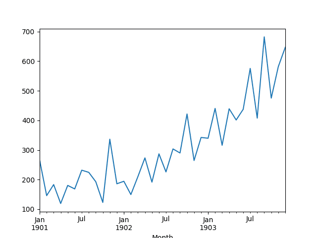
Line Plot of Shampoo Sales Dataset
Next, we will take a look at the model configuration and test harness used in the experiment.
Data Preparation and Model Evaluation
This section describes data preparation and model evaluation used in this tutorial
Data Split
We will split the Shampoo Sales dataset into two parts: a training and a test set.
The first two years of data will be taken for the training dataset and the remaining one year of data will be used for the test set.
Models will be developed using the training dataset and will make predictions on the test dataset.
For reference, the last 12 months of observations are as follows:
|
1 2 3 4 5 6 7 8 9 10 11 12 |
"3-01",339.7 "3-02",440.4 "3-03",315.9 "3-04",439.3 "3-05",401.3 "3-06",437.4 "3-07",575.5 "3-08",407.6 "3-09",682.0 "3-10",475.3 "3-11",581.3 "3-12",646.9 |
Multi-Step Forecast
We will contrive a multi-step forecast.
For a given month in the final 12 months of the dataset, we will be required to make a 3-month forecast.
That is given historical observations (t-1, t-2, … t-n) forecast t, t+1 and t+2.
Specifically, from December in year 2, we must forecast January, February and March. From January, we must forecast February, March and April. All the way to an October, November, December forecast from September in year 3.
A total of 10 3-month forecasts are required, as follows:
|
1 2 3 4 5 6 7 8 9 10 |
Dec, Jan, Feb, Mar Jan, Feb, Mar, Apr Feb, Mar, Apr, May Mar, Apr, May, Jun Apr, May, Jun, Jul May, Jun, Jul, Aug Jun, Jul, Aug, Sep Jul, Aug, Sep, Oct Aug, Sep, Oct, Nov Sep, Oct, Nov, Dec |
Model Evaluation
A rolling-forecast scenario will be used, also called walk-forward model validation.
Each time step of the test dataset will be walked one at a time. A model will be used to make a forecast for the time step, then the actual expected value for the next month from the test set will be taken and made available to the model for the forecast on the next time step.
This mimics a real-world scenario where new Shampoo Sales observations would be available each month and used in the forecasting of the following month.
This will be simulated by the structure of the train and test datasets.
All forecasts on the test dataset will be collected and an error score calculated to summarize the skill of the model for each of the forecast time steps. The root mean squared error (RMSE) will be used as it punishes large errors and results in a score that is in the same units as the forecast data, namely monthly shampoo sales.
Persistence Model
A good baseline for time series forecasting is the persistence model.
This is a forecasting model where the last observation is persisted forward. Because of its simplicity, it is often called the naive forecast.
You can learn more about the persistence model for time series forecasting in the post:
Prepare Data
The first step is to transform the data from a series into a supervised learning problem.
That is to go from a list of numbers to a list of input and output patterns. We can achieve this using a pre-prepared function called series_to_supervised().
For more on this function, see the post:
The function is listed below.
|
1 2 3 4 5 6 7 8 9 10 11 12 13 14 15 16 17 18 19 20 21 22 23 |
# convert time series into supervised learning problem def series_to_supervised(data, n_in=1, n_out=1, dropnan=True): n_vars = 1 if type(data) is list else data.shape[1] df = DataFrame(data) cols, names = list(), list() # input sequence (t-n, ... t-1) for i in range(n_in, 0, -1): cols.append(df.shift(i)) names += [('var%d(t-%d)' % (j+1, i)) for j in range(n_vars)] # forecast sequence (t, t+1, ... t+n) for i in range(0, n_out): cols.append(df.shift(-i)) if i == 0: names += [('var%d(t)' % (j+1)) for j in range(n_vars)] else: names += [('var%d(t+%d)' % (j+1, i)) for j in range(n_vars)] # put it all together agg = concat(cols, axis=1) agg.columns = names # drop rows with NaN values if dropnan: agg.dropna(inplace=True) return agg |
The function can be called by passing in the loaded series values an n_in value of 1 and an n_out value of 3; for example:
|
1 |
supervised = series_to_supervised(raw_values, 1, 3) |
Next, we can split the supervised learning dataset into training and test sets.
We know that in this form, the last 10 rows contain data for the final year. These rows comprise the test set and the rest of the data makes up the training dataset.
We can put all of this together in a new function that takes the loaded series and some parameters and returns a train and test set ready for modeling.
|
1 2 3 4 5 6 7 8 9 10 11 |
# transform series into train and test sets for supervised learning def prepare_data(series, n_test, n_lag, n_seq): # extract raw values raw_values = series.values raw_values = raw_values.reshape(len(raw_values), 1) # transform into supervised learning problem X, y supervised = series_to_supervised(raw_values, n_lag, n_seq) supervised_values = supervised.values # split into train and test sets train, test = supervised_values[0:-n_test], supervised_values[-n_test:] return train, test |
We can test this with the Shampoo dataset. The complete example is listed below.
|
1 2 3 4 5 6 7 8 9 10 11 12 13 14 15 16 17 18 19 20 21 22 23 24 25 26 27 28 29 30 31 32 33 34 35 36 37 38 39 40 41 42 43 44 45 46 47 48 49 50 51 52 53 54 55 |
from pandas import DataFrame from pandas import concat from pandas import read_csv from pandas import datetime # date-time parsing function for loading the dataset def parser(x): return datetime.strptime('190'+x, '%Y-%m') # convert time series into supervised learning problem def series_to_supervised(data, n_in=1, n_out=1, dropnan=True): n_vars = 1 if type(data) is list else data.shape[1] df = DataFrame(data) cols, names = list(), list() # input sequence (t-n, ... t-1) for i in range(n_in, 0, -1): cols.append(df.shift(i)) names += [('var%d(t-%d)' % (j+1, i)) for j in range(n_vars)] # forecast sequence (t, t+1, ... t+n) for i in range(0, n_out): cols.append(df.shift(-i)) if i == 0: names += [('var%d(t)' % (j+1)) for j in range(n_vars)] else: names += [('var%d(t+%d)' % (j+1, i)) for j in range(n_vars)] # put it all together agg = concat(cols, axis=1) agg.columns = names # drop rows with NaN values if dropnan: agg.dropna(inplace=True) return agg # transform series into train and test sets for supervised learning def prepare_data(series, n_test, n_lag, n_seq): # extract raw values raw_values = series.values raw_values = raw_values.reshape(len(raw_values), 1) # transform into supervised learning problem X, y supervised = series_to_supervised(raw_values, n_lag, n_seq) supervised_values = supervised.values # split into train and test sets train, test = supervised_values[0:-n_test], supervised_values[-n_test:] return train, test # load dataset series = read_csv('shampoo-sales.csv', header=0, parse_dates=[0], index_col=0, squeeze=True, date_parser=parser) # configure n_lag = 1 n_seq = 3 n_test = 10 # prepare data train, test = prepare_data(series, n_test, n_lag, n_seq) print(test) print('Train: %s, Test: %s' % (train.shape, test.shape)) |
Running the example first prints the entire test dataset, which is the last 10 rows. The shape and size of the train test datasets is also printed.
|
1 2 3 4 5 6 7 8 9 10 11 |
[[ 342.3 339.7 440.4 315.9] [ 339.7 440.4 315.9 439.3] [ 440.4 315.9 439.3 401.3] [ 315.9 439.3 401.3 437.4] [ 439.3 401.3 437.4 575.5] [ 401.3 437.4 575.5 407.6] [ 437.4 575.5 407.6 682. ] [ 575.5 407.6 682. 475.3] [ 407.6 682. 475.3 581.3] [ 682. 475.3 581.3 646.9]] Train: (23, 4), Test: (10, 4) |
We can see the single input value (first column) on the first row of the test dataset matches the observation in the shampoo-sales for December in the 2nd year:
|
1 |
"2-12",342.3 |
We can also see that each row contains 4 columns for the 1 input and 3 output values in each observation.
Make Forecasts
The next step is to make persistence forecasts.
We can implement the persistence forecast easily in a function named persistence() that takes the last observation and the number of forecast steps to persist. This function returns an array containing the forecast.
|
1 2 3 |
# make a persistence forecast def persistence(last_ob, n_seq): return [last_ob for i in range(n_seq)] |
We can then call this function for each time step in the test dataset from December in year 2 to September in year 3.
Below is a function make_forecasts() that does this and takes the train, test, and configuration for the dataset as arguments and returns a list of forecasts.
|
1 2 3 4 5 6 7 8 9 10 |
# evaluate the persistence model def make_forecasts(train, test, n_lag, n_seq): forecasts = list() for i in range(len(test)): X, y = test[i, 0:n_lag], test[i, n_lag:] # make forecast forecast = persistence(X[-1], n_seq) # store the forecast forecasts.append(forecast) return forecasts |
We can call this function as follows:
|
1 |
forecasts = make_forecasts(train, test, 1, 3) |
Evaluate Forecasts
The final step is to evaluate the forecasts.
We can do that by calculating the RMSE for each time step of the multi-step forecast, in this case giving us 3 RMSE scores. The function below, evaluate_forecasts(), calculates and prints the RMSE for each forecasted time step.
|
1 2 3 4 5 6 7 |
# evaluate the RMSE for each forecast time step def evaluate_forecasts(test, forecasts, n_lag, n_seq): for i in range(n_seq): actual = test[:,(n_lag+i)] predicted = [forecast[i] for forecast in forecasts] rmse = sqrt(mean_squared_error(actual, predicted)) print('t+%d RMSE: %f' % ((i+1), rmse)) |
We can call it as follows:
|
1 |
evaluate_forecasts(test, forecasts, 1, 3) |
It is also helpful to plot the forecasts in the context of the original dataset to get an idea of how the RMSE scores relate to the problem in context.
We can first plot the entire Shampoo dataset, then plot each forecast as a red line. The function plot_forecasts() below will create and show this plot.
|
1 2 3 4 5 6 7 8 9 10 11 12 |
# plot the forecasts in the context of the original dataset def plot_forecasts(series, forecasts, n_test): # plot the entire dataset in blue pyplot.plot(series.values) # plot the forecasts in red for i in range(len(forecasts)): off_s = len(series) - n_test + i off_e = off_s + len(forecasts[i]) xaxis = [x for x in range(off_s, off_e)] pyplot.plot(xaxis, forecasts[i], color='red') # show the plot pyplot.show() |
We can call the function as follows. Note that the number of observations held back on the test set is 12 for the 12 months, as opposed to 10 for the 10 supervised learning input/output patterns as was used above.
|
1 2 |
# plot forecasts plot_forecasts(series, forecasts, 12) |
We can make the plot better by connecting the persisted forecast to the actual persisted value in the original dataset.
This will require adding the last observed value to the front of the forecast. Below is an updated version of the plot_forecasts() function with this improvement.
|
1 2 3 4 5 6 7 8 9 10 11 12 13 |
# plot the forecasts in the context of the original dataset def plot_forecasts(series, forecasts, n_test): # plot the entire dataset in blue pyplot.plot(series.values) # plot the forecasts in red for i in range(len(forecasts)): off_s = len(series) - 12 + i - 1 off_e = off_s + len(forecasts[i]) + 1 xaxis = [x for x in range(off_s, off_e)] yaxis = [series.values[off_s]] + forecasts[i] pyplot.plot(xaxis, yaxis, color='red') # show the plot pyplot.show() |
Complete Example
We can put all of these pieces together.
The complete code example for the multi-step persistence forecast is listed below.
|
1 2 3 4 5 6 7 8 9 10 11 12 13 14 15 16 17 18 19 20 21 22 23 24 25 26 27 28 29 30 31 32 33 34 35 36 37 38 39 40 41 42 43 44 45 46 47 48 49 50 51 52 53 54 55 56 57 58 59 60 61 62 63 64 65 66 67 68 69 70 71 72 73 74 75 76 77 78 79 80 81 82 83 84 85 86 87 88 89 90 91 92 93 94 95 96 97 98 99 |
from pandas import DataFrame from pandas import concat from pandas import read_csv from pandas import datetime from sklearn.metrics import mean_squared_error from math import sqrt from matplotlib import pyplot # date-time parsing function for loading the dataset def parser(x): return datetime.strptime('190'+x, '%Y-%m') # convert time series into supervised learning problem def series_to_supervised(data, n_in=1, n_out=1, dropnan=True): n_vars = 1 if type(data) is list else data.shape[1] df = DataFrame(data) cols, names = list(), list() # input sequence (t-n, ... t-1) for i in range(n_in, 0, -1): cols.append(df.shift(i)) names += [('var%d(t-%d)' % (j+1, i)) for j in range(n_vars)] # forecast sequence (t, t+1, ... t+n) for i in range(0, n_out): cols.append(df.shift(-i)) if i == 0: names += [('var%d(t)' % (j+1)) for j in range(n_vars)] else: names += [('var%d(t+%d)' % (j+1, i)) for j in range(n_vars)] # put it all together agg = concat(cols, axis=1) agg.columns = names # drop rows with NaN values if dropnan: agg.dropna(inplace=True) return agg # transform series into train and test sets for supervised learning def prepare_data(series, n_test, n_lag, n_seq): # extract raw values raw_values = series.values raw_values = raw_values.reshape(len(raw_values), 1) # transform into supervised learning problem X, y supervised = series_to_supervised(raw_values, n_lag, n_seq) supervised_values = supervised.values # split into train and test sets train, test = supervised_values[0:-n_test], supervised_values[-n_test:] return train, test # make a persistence forecast def persistence(last_ob, n_seq): return [last_ob for i in range(n_seq)] # evaluate the persistence model def make_forecasts(train, test, n_lag, n_seq): forecasts = list() for i in range(len(test)): X, y = test[i, 0:n_lag], test[i, n_lag:] # make forecast forecast = persistence(X[-1], n_seq) # store the forecast forecasts.append(forecast) return forecasts # evaluate the RMSE for each forecast time step def evaluate_forecasts(test, forecasts, n_lag, n_seq): for i in range(n_seq): actual = test[:,(n_lag+i)] predicted = [forecast[i] for forecast in forecasts] rmse = sqrt(mean_squared_error(actual, predicted)) print('t+%d RMSE: %f' % ((i+1), rmse)) # plot the forecasts in the context of the original dataset def plot_forecasts(series, forecasts, n_test): # plot the entire dataset in blue pyplot.plot(series.values) # plot the forecasts in red for i in range(len(forecasts)): off_s = len(series) - n_test + i - 1 off_e = off_s + len(forecasts[i]) + 1 xaxis = [x for x in range(off_s, off_e)] yaxis = [series.values[off_s]] + forecasts[i] pyplot.plot(xaxis, yaxis, color='red') # show the plot pyplot.show() # load dataset series = read_csv('shampoo-sales.csv', header=0, parse_dates=[0], index_col=0, squeeze=True, date_parser=parser) # configure n_lag = 1 n_seq = 3 n_test = 10 # prepare data train, test = prepare_data(series, n_test, n_lag, n_seq) # make forecasts forecasts = make_forecasts(train, test, n_lag, n_seq) # evaluate forecasts evaluate_forecasts(test, forecasts, n_lag, n_seq) # plot forecasts plot_forecasts(series, forecasts, n_test+2) |
Running the example first prints the RMSE for each of the forecasted time steps.
Note: Your results may vary given the stochastic nature of the algorithm or evaluation procedure, or differences in numerical precision. Consider running the example a few times and compare the average outcome.
This gives us a baseline of performance on each time step that we would expect the LSTM to outperform.
|
1 2 3 |
t+1 RMSE: 144.535304 t+2 RMSE: 86.479905 t+3 RMSE: 121.149168 |
The plot of the original time series with the multi-step persistence forecasts is also created. The lines connect to the appropriate input value for each forecast.
This context shows how naive the persistence forecasts actually are.
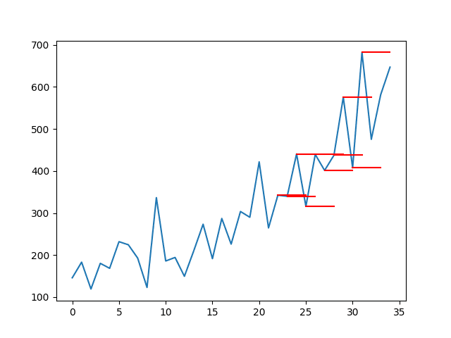
Line Plot of Shampoo Sales Dataset with Multi-Step Persistence Forecasts
Multi-Step LSTM Network
In this section, we will use the persistence example as a starting point and look at the changes needed to fit an LSTM to the training data and make multi-step forecasts for the test dataset.
Prepare Data
The data must be prepared before we can use it to train an LSTM.
Specifically, two additional changes are required:
- Stationary. The data shows an increasing trend that must be removed by differencing.
- Scale. The scale of the data must be reduced to values between -1 and 1, the activation function of the LSTM units.
We can introduce a function to make the data stationary called difference(). This will transform the series of values into a series of differences, a simpler representation to work with.
|
1 2 3 4 5 6 7 |
# create a differenced series def difference(dataset, interval=1): diff = list() for i in range(interval, len(dataset)): value = dataset[i] - dataset[i - interval] diff.append(value) return Series(diff) |
We can use the MinMaxScaler from the sklearn library to scale the data.
Putting this together, we can update the prepare_data() function to first difference the data and rescale it, then perform the transform into a supervised learning problem and train test sets as we did before with the persistence example.
The function now returns a scaler in addition to the train and test datasets.
|
1 2 3 4 5 6 7 8 9 10 11 12 13 14 15 16 17 18 |
# transform series into train and test sets for supervised learning def prepare_data(series, n_test, n_lag, n_seq): # extract raw values raw_values = series.values # transform data to be stationary diff_series = difference(raw_values, 1) diff_values = diff_series.values diff_values = diff_values.reshape(len(diff_values), 1) # rescale values to -1, 1 scaler = MinMaxScaler(feature_range=(-1, 1)) scaled_values = scaler.fit_transform(diff_values) scaled_values = scaled_values.reshape(len(scaled_values), 1) # transform into supervised learning problem X, y supervised = series_to_supervised(scaled_values, n_lag, n_seq) supervised_values = supervised.values # split into train and test sets train, test = supervised_values[0:-n_test], supervised_values[-n_test:] return scaler, train, test |
We can call this function as follows:
|
1 2 |
# prepare data scaler, train, test = prepare_data(series, n_test, n_lag, n_seq) |
Fit LSTM Network
Next, we need to fit an LSTM network model to the training data.
This first requires that the training dataset be transformed from a 2D array [samples, features] to a 3D array [samples, timesteps, features]. We will fix time steps at 1, so this change is straightforward.
Next, we need to design an LSTM network. We will use a simple structure with 1 hidden layer with 1 LSTM unit, then an output layer with linear activation and 3 output values. The network will use a mean squared error loss function and the efficient ADAM optimization algorithm.
The LSTM is stateful; this means that we have to manually reset the state of the network at the end of each training epoch. The network will be fit for 1500 epochs.
The same batch size must be used for training and prediction, and we require predictions to be made at each time step of the test dataset. This means that a batch size of 1 must be used. A batch size of 1 is also called online learning as the network weights will be updated during training after each training pattern (as opposed to mini batch or batch updates).
We can put all of this together in a function called fit_lstm(). The function takes a number of key parameters that can be used to tune the network later and the function returns a fit LSTM model ready for forecasting.
|
1 2 3 4 5 6 7 8 9 10 11 12 13 14 15 |
# fit an LSTM network to training data def fit_lstm(train, n_lag, n_seq, n_batch, nb_epoch, n_neurons): # reshape training into [samples, timesteps, features] X, y = train[:, 0:n_lag], train[:, n_lag:] X = X.reshape(X.shape[0], 1, X.shape[1]) # design network model = Sequential() model.add(LSTM(n_neurons, batch_input_shape=(n_batch, X.shape[1], X.shape[2]), stateful=True)) model.add(Dense(y.shape[1])) model.compile(loss='mean_squared_error', optimizer='adam') # fit network for i in range(nb_epoch): model.fit(X, y, epochs=1, batch_size=n_batch, verbose=0, shuffle=False) model.reset_states() return model |
The function can be called as follows:
|
1 2 |
# fit model model = fit_lstm(train, 1, 3, 1, 1500, 1) |
The configuration of the network was not tuned; try different parameters if you like.
Report your findings in the comments below. I’d love to see what you can get.
Make LSTM Forecasts
The next step is to use the fit LSTM network to make forecasts.
A single forecast can be made with the fit LSTM network by calling model.predict(). Again, the data must be formatted into a 3D array with the format [samples, timesteps, features].
We can wrap this up into a function called forecast_lstm().
|
1 2 3 4 5 6 7 8 |
# make one forecast with an LSTM, def forecast_lstm(model, X, n_batch): # reshape input pattern to [samples, timesteps, features] X = X.reshape(1, 1, len(X)) # make forecast forecast = model.predict(X, batch_size=n_batch) # convert to array return [x for x in forecast[0, :]] |
We can call this function from the make_forecasts() function and update it to accept the model as an argument. The updated version is listed below.
|
1 2 3 4 5 6 7 8 9 10 |
# evaluate the persistence model def make_forecasts(model, n_batch, train, test, n_lag, n_seq): forecasts = list() for i in range(len(test)): X, y = test[i, 0:n_lag], test[i, n_lag:] # make forecast forecast = forecast_lstm(model, X, n_batch) # store the forecast forecasts.append(forecast) return forecasts |
This updated version of the make_forecasts() function can be called as follows:
|
1 2 |
# make forecasts forecasts = make_forecasts(model, 1, train, test, 1, 3) |
Invert Transforms
After the forecasts have been made, we need to invert the transforms to return the values back into the original scale.
This is needed so that we can calculate error scores and plots that are comparable with other models, like the persistence forecast above.
We can invert the scale of the forecasts directly using the MinMaxScaler object that offers an inverse_transform() function.
We can invert the differencing by adding the value of the last observation (prior months’ shampoo sales) to the first forecasted value, then propagating the value down the forecast.
This is a little fiddly; we can wrap up the behavior in a function name inverse_difference() that takes the last observed value prior to the forecast and the forecast as arguments and returns the inverted forecast.
|
1 2 3 4 5 6 7 8 9 |
# invert differenced forecast def inverse_difference(last_ob, forecast): # invert first forecast inverted = list() inverted.append(forecast[0] + last_ob) # propagate difference forecast using inverted first value for i in range(1, len(forecast)): inverted.append(forecast[i] + inverted[i-1]) return inverted |
Putting this together, we can create an inverse_transform() function that works through each forecast, first inverting the scale and then inverting the differences, returning forecasts to their original scale.
|
1 2 3 4 5 6 7 8 9 10 11 12 13 14 15 16 17 |
# inverse data transform on forecasts def inverse_transform(series, forecasts, scaler, n_test): inverted = list() for i in range(len(forecasts)): # create array from forecast forecast = array(forecasts[i]) forecast = forecast.reshape(1, len(forecast)) # invert scaling inv_scale = scaler.inverse_transform(forecast) inv_scale = inv_scale[0, :] # invert differencing index = len(series) - n_test + i - 1 last_ob = series.values[index] inv_diff = inverse_difference(last_ob, inv_scale) # store inverted.append(inv_diff) return inverted |
We can call this function with the forecasts as follows:
|
1 2 |
# inverse transform forecasts and test forecasts = inverse_transform(series, forecasts, scaler, n_test+2) |
We can also invert the transforms on the output part test dataset so that we can correctly calculate the RMSE scores, as follows:
|
1 2 |
actual = [row[n_lag:] for row in test] actual = inverse_transform(series, actual, scaler, n_test+2) |
We can also simplify the calculation of RMSE scores to expect the test data to only contain the output values, as follows:
|
1 2 3 4 5 6 |
def evaluate_forecasts(test, forecasts, n_lag, n_seq): for i in range(n_seq): actual = [row[i] for row in test] predicted = [forecast[i] for forecast in forecasts] rmse = sqrt(mean_squared_error(actual, predicted)) print('t+%d RMSE: %f' % ((i+1), rmse)) |
Complete Example
We can tie all of these pieces together and fit an LSTM network to the multi-step time series forecasting problem.
The complete code listing is provided below.
|
1 2 3 4 5 6 7 8 9 10 11 12 13 14 15 16 17 18 19 20 21 22 23 24 25 26 27 28 29 30 31 32 33 34 35 36 37 38 39 40 41 42 43 44 45 46 47 48 49 50 51 52 53 54 55 56 57 58 59 60 61 62 63 64 65 66 67 68 69 70 71 72 73 74 75 76 77 78 79 80 81 82 83 84 85 86 87 88 89 90 91 92 93 94 95 96 97 98 99 100 101 102 103 104 105 106 107 108 109 110 111 112 113 114 115 116 117 118 119 120 121 122 123 124 125 126 127 128 129 130 131 132 133 134 135 136 137 138 139 140 141 142 143 144 145 146 147 148 149 150 151 152 153 154 155 156 157 158 159 160 161 162 163 164 165 166 167 168 169 170 171 172 173 174 175 176 177 178 |
from pandas import DataFrame from pandas import Series from pandas import concat from pandas import read_csv from pandas import datetime from sklearn.metrics import mean_squared_error from sklearn.preprocessing import MinMaxScaler from keras.models import Sequential from keras.layers import Dense from keras.layers import LSTM from math import sqrt from matplotlib import pyplot from numpy import array # date-time parsing function for loading the dataset def parser(x): return datetime.strptime('190'+x, '%Y-%m') # convert time series into supervised learning problem def series_to_supervised(data, n_in=1, n_out=1, dropnan=True): n_vars = 1 if type(data) is list else data.shape[1] df = DataFrame(data) cols, names = list(), list() # input sequence (t-n, ... t-1) for i in range(n_in, 0, -1): cols.append(df.shift(i)) names += [('var%d(t-%d)' % (j+1, i)) for j in range(n_vars)] # forecast sequence (t, t+1, ... t+n) for i in range(0, n_out): cols.append(df.shift(-i)) if i == 0: names += [('var%d(t)' % (j+1)) for j in range(n_vars)] else: names += [('var%d(t+%d)' % (j+1, i)) for j in range(n_vars)] # put it all together agg = concat(cols, axis=1) agg.columns = names # drop rows with NaN values if dropnan: agg.dropna(inplace=True) return agg # create a differenced series def difference(dataset, interval=1): diff = list() for i in range(interval, len(dataset)): value = dataset[i] - dataset[i - interval] diff.append(value) return Series(diff) # transform series into train and test sets for supervised learning def prepare_data(series, n_test, n_lag, n_seq): # extract raw values raw_values = series.values # transform data to be stationary diff_series = difference(raw_values, 1) diff_values = diff_series.values diff_values = diff_values.reshape(len(diff_values), 1) # rescale values to -1, 1 scaler = MinMaxScaler(feature_range=(-1, 1)) scaled_values = scaler.fit_transform(diff_values) scaled_values = scaled_values.reshape(len(scaled_values), 1) # transform into supervised learning problem X, y supervised = series_to_supervised(scaled_values, n_lag, n_seq) supervised_values = supervised.values # split into train and test sets train, test = supervised_values[0:-n_test], supervised_values[-n_test:] return scaler, train, test # fit an LSTM network to training data def fit_lstm(train, n_lag, n_seq, n_batch, nb_epoch, n_neurons): # reshape training into [samples, timesteps, features] X, y = train[:, 0:n_lag], train[:, n_lag:] X = X.reshape(X.shape[0], 1, X.shape[1]) # design network model = Sequential() model.add(LSTM(n_neurons, batch_input_shape=(n_batch, X.shape[1], X.shape[2]), stateful=True)) model.add(Dense(y.shape[1])) model.compile(loss='mean_squared_error', optimizer='adam') # fit network for i in range(nb_epoch): model.fit(X, y, epochs=1, batch_size=n_batch, verbose=0, shuffle=False) model.reset_states() return model # make one forecast with an LSTM, def forecast_lstm(model, X, n_batch): # reshape input pattern to [samples, timesteps, features] X = X.reshape(1, 1, len(X)) # make forecast forecast = model.predict(X, batch_size=n_batch) # convert to array return [x for x in forecast[0, :]] # evaluate the persistence model def make_forecasts(model, n_batch, train, test, n_lag, n_seq): forecasts = list() for i in range(len(test)): X, y = test[i, 0:n_lag], test[i, n_lag:] # make forecast forecast = forecast_lstm(model, X, n_batch) # store the forecast forecasts.append(forecast) return forecasts # invert differenced forecast def inverse_difference(last_ob, forecast): # invert first forecast inverted = list() inverted.append(forecast[0] + last_ob) # propagate difference forecast using inverted first value for i in range(1, len(forecast)): inverted.append(forecast[i] + inverted[i-1]) return inverted # inverse data transform on forecasts def inverse_transform(series, forecasts, scaler, n_test): inverted = list() for i in range(len(forecasts)): # create array from forecast forecast = array(forecasts[i]) forecast = forecast.reshape(1, len(forecast)) # invert scaling inv_scale = scaler.inverse_transform(forecast) inv_scale = inv_scale[0, :] # invert differencing index = len(series) - n_test + i - 1 last_ob = series.values[index] inv_diff = inverse_difference(last_ob, inv_scale) # store inverted.append(inv_diff) return inverted # evaluate the RMSE for each forecast time step def evaluate_forecasts(test, forecasts, n_lag, n_seq): for i in range(n_seq): actual = [row[i] for row in test] predicted = [forecast[i] for forecast in forecasts] rmse = sqrt(mean_squared_error(actual, predicted)) print('t+%d RMSE: %f' % ((i+1), rmse)) # plot the forecasts in the context of the original dataset def plot_forecasts(series, forecasts, n_test): # plot the entire dataset in blue pyplot.plot(series.values) # plot the forecasts in red for i in range(len(forecasts)): off_s = len(series) - n_test + i - 1 off_e = off_s + len(forecasts[i]) + 1 xaxis = [x for x in range(off_s, off_e)] yaxis = [series.values[off_s]] + forecasts[i] pyplot.plot(xaxis, yaxis, color='red') # show the plot pyplot.show() # load dataset series = read_csv('shampoo-sales.csv', header=0, parse_dates=[0], index_col=0, squeeze=True, date_parser=parser) # configure n_lag = 1 n_seq = 3 n_test = 10 n_epochs = 1500 n_batch = 1 n_neurons = 1 # prepare data scaler, train, test = prepare_data(series, n_test, n_lag, n_seq) # fit model model = fit_lstm(train, n_lag, n_seq, n_batch, n_epochs, n_neurons) # make forecasts forecasts = make_forecasts(model, n_batch, train, test, n_lag, n_seq) # inverse transform forecasts and test forecasts = inverse_transform(series, forecasts, scaler, n_test+2) actual = [row[n_lag:] for row in test] actual = inverse_transform(series, actual, scaler, n_test+2) # evaluate forecasts evaluate_forecasts(actual, forecasts, n_lag, n_seq) # plot forecasts plot_forecasts(series, forecasts, n_test+2) |
Running the example first prints the RMSE for each of the forecasted time steps.
Note: Your results may vary given the stochastic nature of the algorithm or evaluation procedure, or differences in numerical precision. Consider running the example a few times and compare the average outcome.
We can see that the scores at each forecasted time step are better, in some cases much better, than the persistence forecast.
This shows that the configured LSTM does have skill on the problem.
It is interesting to note that the RMSE does not become progressively worse with the length of the forecast horizon, as would be expected. This is marked by the fact that the t+2 appears easier to forecast than t+1. This may be because the downward tick is easier to predict than the upward tick noted in the series (this could be confirmed with more in-depth analysis of the results).
|
1 2 3 |
t+1 RMSE: 95.973221 t+2 RMSE: 78.872348 t+3 RMSE: 105.613951 |
A line plot of the series (blue) with the forecasts (red) is also created.
The plot shows that although the skill of the model is better, some of the forecasts are not very good and that there is plenty of room for improvement.
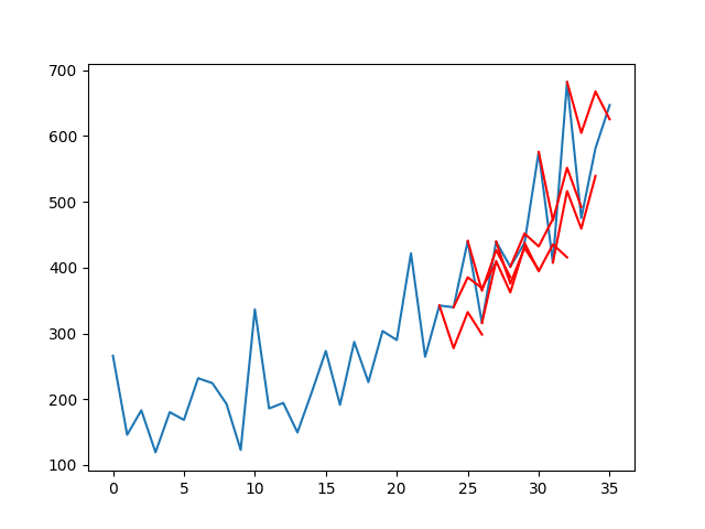
Line Plot of Shampoo Sales Dataset with Multi-Step LSTM Forecasts
Extensions
There are some extensions you may consider if you are looking to push beyond this tutorial.
- Update LSTM. Change the example to refit or update the LSTM as new data is made available. A 10s of training epochs should be sufficient to retrain with a new observation.
- Tune the LSTM. Grid search some of the LSTM parameters used in the tutorial, such as number of epochs, number of neurons, and number of layers to see if you can further lift performance.
- Seq2Seq. Use the encoder-decoder paradigm for LSTMs to forecast each sequence to see if this offers any benefit.
- Time Horizon. Experiment with forecasting different time horizons and see how the behavior of the network varies at different lead times.
Did you try any of these extensions?
Share your results in the comments; I’d love to hear about it.
Summary
In this tutorial, you discovered how to develop LSTM networks for multi-step time series forecasting.
Specifically, you learned:
- How to develop a persistence model for multi-step time series forecasting.
- How to develop an LSTM network for multi-step time series forecasting.
- How to evaluate and plot the results from multi-step time series forecasting.
Do you have any questions about multi-step time series forecasting with LSTMs?
Ask your questions in the comments below and I will do my best to answer.
Develop Deep Learning models for Time Series Today!

Develop Your Own Forecasting models in Minutes
...with just a few lines of python code
Discover how in my new Ebook:
Deep Learning for Time Series Forecasting
It provides self-study tutorials on topics like:
CNNs, LSTMs,
Multivariate Forecasting, Multi-Step Forecasting and much more...
Finally Bring Deep Learning to your Time Series Forecasting Projects
Skip the Academics. Just Results.


Thanks
you are the best
Did not had to wait for long. Asked for it in different blog few days back
I hope you find the post useful!
I believe so. Things are getting deeper here.
Will we get recursive LSTM MODEL for multi step forecasting soon?
Will eagerly wait for that blog.
Thanks
Maybe.
Sir,
Hope to see that soon.
Hi Masum,
I’m studying LSTM on website( https://machinelearningmastery.com/multi-step-time-series-forecasting-long-short-term-memory-networks-python/ )and found you on message board. Do you have any idea about Muti-step forecast? I run the code of the tutorial, but always got a over-fitting results using the history data.
Thank you and looking forward for your reply.
when you predict by using the recursive LSTM model, can you get a relatively precise result?
I find it’s hard to get satisfying outcomes, maybe I am not good at training the model like that.
Hi, I’m completely new to RNN and neural networks. I have a project in hand with 9 years of monthly sales data of a project. I want to apply LSTM to forecast into future 6-7 months.
I’ve used ARIMA and got a decent accuracy. But I want to try LSTM after reading so many articles in its favour.
it is a uni-variate (contains sales history for 9 years monthly data) consistent time series data.
Can you suggest me where should I start learning? or should I use this blog directly on my data.
Your earliest response will be deeply appreciated.
And thanks for all your blogs. They really help.
I recommend starting here:
https://machinelearningmastery.com/start-here/#deep_learning_time_series
I am not sure why you would call the following multiple times with the SAME parameter?
model.fit(X, y, epochs=1, batch_size=n_batch, verbose=0, shuffle=False)
model.reset_states()
Shall X, and y actually need to be indexed by i at different epoch?
This is the standard process for training a neural net, e.g. showing the same dataset for multiple epochs, in this case we re doing so manually rather than automatically by the framework.
Thanks a lot for this post. I was trying to make this for my thesis since september, with no well results. But I’m having trouble: I’m not able to compile. Maybe you or someone who reads this is able to tell me why this happens: I’m getting the following error when running the code:
The TensorFlow library wasn’t compiled to use SSE instructions, but these are available on your machine and could speed up CPU computations.
The TensorFlow library wasn’t compiled to use SSE2 instructions, but these are available on your machine and could speed up CPU computations.
The TensorFlow library wasn’t compiled to use SSE3 instructions, but these are available on your machine and could speed up CPU computations.
.
The TensorFlow library wasn’t compiled to use SSE4.1 instructions, but these are available on your machine and could speed up CPU computations.
The TensorFlow library wasn’t compiled to use SSE4.2 instructions, but these are available on your machine and could speed up CPU computations.
The TensorFlow library wasn’t compiled to use AVX instructions, but these are available on your machine and could speed up CPU computations.
Obviously it has something to do with Tensorflow (I have read about this problem and I think its becase is not installed on source, but have no idea about how to fix it).
Thank you in advance.
These are warnings that you can ignore.
Sir,
Can we say that multiple output strategy ( avoiding 1.direct, 2. Recursive, 3.direct recursive hybrid strategies) have been used here ?
Am I right ?
I think the LSTM has implemented a direct strategy.
sir,
what can be done to make it iterative strategy? any example of code would be great.
Isn’t this a multiple output strategy?
From my understanding the number of outputs is built into the model. You feed it one sample and it returns the whole output based on that.
This model will produce a vector output.
An encoder-decoder would produce one time step at a time as output.
Do you have any code for seq2seq?
Yes, I have general examples on my blog, you can start here:
https://machinelearningmastery.com/start-here/#lstm
I have examples of seq2seq for time series forecasting in this book:
https://machinelearningmastery.com/deep-learning-for-time-series-forecasting/
Hi,Jason,
Your article is very useful! I have a problem, if the data series are three-dimensional data, the 2th line is the put -in data,and the 3th line is the forecasting data(all include the train and test data ),Do they can run the” difference”and “tansform”?
Thank you very much!
Great question.
You may want to only make the prediction variable stationary. Consider perform three tests:
– Model as-is
– Model with output variable stationary
– Model with all variables stationary (if others are non-stationary)
I have discovered how to do it by asking some people. The object series is actually a Pandas Series. It’s a vector of information, with a named index. Your dataset, however, contains two fields of information, in addition to the time series index, which makes it a DataFrame. This is the reason why the tutorial code breaks with your data.
To pass your entire dataset to MinMaxScaler, just run difference() on both columns and pass in the transformed vectors for scaling. MinMaxScaler accepts an n-dimensional DataFrame object:
ncol = 2
diff_df = pd.concat([difference(df[i], 1) for i in range(1,ncol+1)], axis=1)
scaler = MinMaxScaler(feature_range=(0, 1))
scaled_values = scaler.fit_transform(diff_df)
So, with this, we can use as many variables as we want. But now I have a big doubt.
When the transform or dataset into a supervised learning problem, we have a distribution in columns as shown in https://machinelearningmastery.com/convert-time-series-supervised-learning-problem-python/
I mean, for a 2 variables dataset as yours, we can set, for example, this values:
n_lags=1
n_seq=2
so we will have a supervised dataset like this:
var1(t-1) var2(t-1) var1(t) var2 (t) var1(t+1) var2 (t+1)
so, if we want to train the ANN to forecast var2 (which is the target we want to predict) with the var1 as input and the previous values of var2 also as input, we have to separate them and here is where my doubt begins.
In the part of the code:
def fit_lstm(train, n_lag, n_seq, n_batch, nb_epoch, n_neurons):
# reshape training into [samples, timesteps, features]
X, y = train[:, 0:n_lag], train[:, n_lag:]
X = X.reshape(X.shape[0], 1, X.shape[1])
I think that if we want to define X, we should use:
X=train[:,0:n_lag*n_vars]
this means we are selecting this as X from the previous example:
var1(t-1) var2(t-1)
(number of lags*number of variables), so: X=train[:,0:1*2]=train[:,0:2]
but…
Y=train[:,n_lag*n_vars:] is the vector of ¿targets?
the problem is that, on this way, we are selecting this as targets:
var1(t) var2(t) var1(t+1) var2(t+1)
so we are including var1 (which we don’t have the aim to forecast, just use as input).
I would like to know if there is any solution to solve this in order to use the variable 1,2…n-1 just as input but not forecasting it.
Hope this is clear :/
Thanks for the previous clarification. I have a dubt in relation to the section “fit network” in the code. I’m having some trouble trying to plot the training graph (validation vs training) in order to see if the network is or not overfitted, but due to the “model.reset_states()” sentence, i can only save the last loss and val_loss from de history sentence. Is there any way to solve this?
thank you in advance 🙂
I reply to myself, if someone is also interested.
Just creating 2 list (or 1, but i see it more clear on this way) and returning then on the function. Then, outside, just plot them. I’m sorry for the question, maybe the answer is obvious, but I’m starting on python and I’m not a programmer.
# fit network
loss=list()
val_loss=list()
for i in range(nb_epoch):
history=model.fit(X, y, epochs=1, batch_size=n_batch,shuffle=True, validation_split=val_split)
eqm=history.history[‘loss’]
eqm_val=history.history[‘val_loss’]
loss.append(eqm)
val_loss.append(eqm_val)
model.reset_states()
return model,loss,val_loss
# fit model
model,loss,val_loss=fit_lstm(train, n_lag, n_seq, n_batch, n_epochs, n_neurons)
pyplot.figure()
pyplot.plot(loss)
pyplot.plot(val_loss)
pyplot.title(‘cross validation’)
pyplot.ylabel(‘MSE’)
pyplot.xlabel(‘epoch’)
pyplot.legend([‘training’, ‘test’], loc=’upper left’)
pyplot.show()
Nice to see you got there jvr, well done.
Hi jrv,
I know this is a lot later but I was wondering whether you still have the full code for when you implemented a multivariate solution for this?
If anyone else has a solution for a multivariate and multi-lagged input to predict just one column I would be very happy to talk!
Thanks in advance
I many new tutorials on the topic, you can get started here:
https://machinelearningmastery.com/start-here/#deep_learning_time_series
History is returned when calling model.fit().
We are only fitting one epoch at a time, so you can retrieve and accumulate performance each epoch in the epoch loop then do something with the data (save/graph/return it) at the end of the loop.
Does that help?
It does help, thank you.
Now I’m trying to find a way to make the training process faster and reduce RMSE, but it’s pretty dificult (the idea is to make results better than in the NARx model implemented in the Matlab Neural Toolbox, but results and computational time are hard to overcome).
LSTMs often need to be trained longer than you think and can greatly benefit from regularization.
Hi,
Thanks for the great tutorial, I’m wondering if you can help me clarify the reason you have
model.reset_states()
(line 83)
when fitting the model, I was able to achieve similar results without the line as well.
Thanks!
It clears the internal state of the LSTM.
I have tried experimenting with and without mode.reset_states(), using some other dataset.
I am doing multistep prediction for 6-10 steps, I am able to get better results without model.reset_states().
Am i doing something wrong, or it completely depends on dataset to dataset.
Thanks in advance.
It completely depends on the dataset and the model.
Thank you so much. 🙂
Thanks for the quick reply Jason :-). I’ve seen other places where reset is done by using callbacks parameter in model.fit.
class ResetStatesCallback(Callback):

    def __init__(self):

        self.counter = 0
def on_batch_begin(self, batch, logs={}):
if self.counter % max_len == 0:
self.model.reset_states()
self.counter += 1
Then the callback is used by as follows:
model.fit(X, y, epochs=1, batch_size=1, verbose=2,

                    shuffle=False, callbacks=[ResetStatesCallback()])
The ResetStatesCallback snippet was obtained from:
http://philipperemy.github.io/keras-stateful-lstm/
Please let me know what you think.
Thanks!
Yes, there are many ways to implement the reset. Use what works best for your application.
Hi Jason, greate post, and I have some questions:
1. in your fit_lstm function, you reset each epoch state, why?
2. why you iterate each epoch by yourself, instead of using model.fit(X, y, epochs)
thx Jason
# fit an LSTM network to training data
def fit_lstm(train, n_lag, n_seq, n_batch, nb_epoch, n_neurons):
# reshape training into [samples, timesteps, features]
X, y = train[:, 0:n_lag], train[:, n_lag:]
X = X.reshape(X.shape[0], 1, X.shape[1])
# design network
model = Sequential()
model.add(LSTM(n_neurons, batch_input_shape=(n_batch, X.shape[1], X.shape[2]), stateful=True))
model.add(Dense(y.shape[1]))
model.compile(loss=’mean_squared_error’, optimizer=’adam’)
# fit network
for i in range(nb_epoch):
model.fit(X, y, epochs=1, batch_size=n_batch, verbose=0, shuffle=False)
model.reset_states()
return model
The end of the epoch is the end of the sequence and the internal state should not carry over to the start of the sequence on the next epoch.
I run the epochs manually to give fine grained control over when resets occur (by default they occur at the end of each batch).
I’d like to clarify line 99 in the LSTM example:
—– plot_forecasts(series, forecasts, n_test+2)
Is the n_test + 2 == n_test + n_lag – n_seq?
Thanks,
J
I’d also like to know why using n_test + 2
I thought it should be n_test + 2 == n_test+n_seq-1 (regardless of n_seq). It would be great if someone could clarify that.
M, you are right. Otherwise the RMS is incorrectly calculated and plotting is not aligned.
I would also very much like to see why n_test + 2 is used
Hi jason,
When I applied your code into a 22-year daily time series, I find out that the LSTM forecast result is similar to persistence one, i.e. the red line is just a horizontal bar. I’m sure I did not mess those two methods, I wonder what cause this?
My key configure as follows:
n_lag = 1
n_seq = 3
n_test = 365*3
and my series length is 8035.
You will need to tune the model to your problem.
Thanks to your tutorial, I’ve been tuning the parameters such as numbers of epochs and neurons these days. However, I noticed that you mentioned the grid search method to get appropriate parameters, could you please explain how to implement it into LSTM? I’m confused about your examples on some other tutorial which has a model class, seems unfamiliar to me.
See this example on how to grid search with LSTMs manually:
https://machinelearningmastery.com/tune-lstm-hyperparameters-keras-time-series-forecasting/
Thanks, I’ve just finished one test. What does it mean if error oscillates violently with epochs increasing instead of steady diminishing? Can I tune the model better, or LSTM is incapable of this time series?
You may need a larger model (more layers and or more neurons).
Jason,
Thank you for these tutorials. These are the best tutorials on the web. One question: what is the best way to forecast the last two values?
Thank you
Thanks MM.
No one can tell you the “best” way to do anything in applied machine learning, you must discover it through trial and error on your specific problem.
Jason,
Understood. Let me re-phrase the question. In a practical application, one would be interested in forecasting the last data point, i.e. in the shampoo dataset, “3-12”. How would you suggest doing that?
Fit your model to all of the data then call predict() passing whatever lag inputs your model requires.
Jason,
Should the line that starts the offset point in plot_forecasts() be
off_s = len(series) – n_test + i + 1
not
off_s = len(series) – n_test + i – 1
Hi Jason,
Thanks for your excellent tutorials!
I have followed a couple of your articles about LSTM and did learn a lot, but here is a question in my mind: can I introduce some interference elements in the model? For example for shampoo sale problem, there may be some data about holiday sales, or sales data after an incident happens. If I want to make prediction for sales after those incidents, what can I do?
What’s more, I noticed that you will parse date/time with a parser, but you did not really introduce time feature into the model. For example I want to make prediction for next Monday or next January, how can I feed time feature?
Thanks!
Yes, see this post for ideas on adding additional features:
https://machinelearningmastery.com/basic-feature-engineering-time-series-data-python/
Thanks for clarification.
I have two more specific questions:
1) In inverse_transform, why index = len(series) – n_test + i – 1?
2) In fit_lstm, you said “reshape training into [samples, timesteps, features]”, but I think the code in line 74 is a little different from your format:
73 X, y = train[:, 0:n_lag], train[:, n_lag:]
74 X = X.reshape(X.shape[0], 1, X.shape[1])
In line 74, I think it should be X = X.reshape(X.shape[0], X.shape[1], 1)
Hi Michael,
Yes, the offset finds one step prior to the forecast in the original time series. I use this motif throughout the tutorial.
In the very next line I say: “We will fix time steps at 1, so this change is straightforward.”
Hi Jason,
Firstly, thanks for all the excellent tutorials.
I’m stepping through this example in detail and have hit the same question as Michael in (2) above. I’m afraid I don’t quite understand the comment “We will fix time steps at 1”.
We need X to have dimensions [samples, timesteps, features]
Therefore, should line 74 not read:
X = X.reshape(X.shape[0], X.shape[1], 1) (as suggested by Michael)
I’m expecting X.shape[1] to be the same as n_lag (i.e. timesteps) and in this example there is only 1 feature.
If, as in your example, timesteps = n_lag = n_features = 1 this wouldn’t make a difference, however, I’m trying with n_lag = 2.
For 1 feature with n_lag = 2 I’m expecting X.shape to be [n_samples, 2, 1] where as the code is giving me [n_samples, 1, 2]
Thanks in advance, Mark.
From memory, both the number of features and number of time steps are 1. They are equilivient.
Also, perhaps this will help:
https://machinelearningmastery.com/faq/single-faq/what-is-the-difference-between-samples-timesteps-and-features-for-lstm-input
Hi Jason,
I would like to know how to do short term and long term prediction with minimum number of models?
For example, I have a 12-step input and 12-step output model A, and a 12-step input and 1-step output model B, would model A gives better prediction for next first time step than model B?
What’s more, if we have 1-step input and 1-step output model, it is more error prone to long term prediction.
if we have multi-step input and 1-step output mode it is still more more error prone long term. So how to regard the long term and short term prediction?
I would recommend developing and evaluating each model for the different uses cases. LSTMs are quite resistant to assumptions and rules of thumb I find in practice.
Hello, thanks for your tutorial
If my prediction model is three time series a, b, c, I would like to use a, b, c to predict the future a, how can I build my LSTM model.
thank you very much!
Each of a, b, and c would be input features. Remember, the shape or dimensions of input data is [samples, timesteps, features].
Does stationarizing data really help the LSTM? If so, what is the intuition behind that? I mean, I can understand that for ARIMA-like methods, but why for LSTM’s?
Yes in my experience, namely because it is a simpler prediction problem.
I would suggest trying a few different “views” of your sequence and see what is easiest to model / gets the best model skill.
Hi Jason,
I want to train a model with the following input size: [6000, 4, 2] ([samples, timestamps, features])
For example, I want to predict shampoo’s sale in next two years. If I have other feature like economy index of every year, can I concatenate sale data and index data in the above format? So my input will be a 3d vector. How should I modify the model to train?
I always get such error: ValueError: Error when checking target: expected dense_1 to have 2 dimensions, but got array with shape (6000, 2, 2).
The error comes from this line: model.fit(X, y, epochs=1, batch_size=n_batch, verbose=0, shuffle=False). Can you provide some advices? Thanks!
Reshape your data to be [6000, 4, 2]
Update the input shape of the network to be (4,2)
Adjust the length of the output sequence you want to predict.
sir,
To make one forecast with an LSTM, if we write
oneforecast = forecast_lstm(model, X, n_batch)
it says: undefined X
what should be the value of X? we know the model and n_batch value?
would you help?
X would be the input sequence required to make a prediction, e.g. lag obs.
sir,
what if I want to tell the model to learn from train data (23 samples here) and want to forecast only 3 steps forward (Jan, Feb, Mar). I want to avoid persistence model in this case and only require 3 step direct strategy. hope you got that.
any help would be grateful.
tarin (past data)= forecast (Jan, Feb, Mar)
Perhaps I misunderstand, but this is the model presented in the tutorial. It predicts 3 time steps ahead.
# evaluate the persistence model
def make_forecasts(model, n_batch, train, test, n_lag, n_seq):
forecasts = list()
for i in range(len(test)):
X, y = test[i, 0:n_lag], test[i, n_lag:]
# make forecast
forecast = forecast_lstm(model, X, n_batch)
# store the forecast
forecasts.append(forecast)
return forecasts
here if i would like to make only one forecast for 3 steps (jan,feb,march) what i have to change. i do not need the rest of the month(april, may, june, july,aug,……dec). one predictions or forecast for 3 steps.
hope you got me
Pass in only what is required to make the prediction for those 3 months.
sir,
will be kind enough to simplify a little bit more.
I did not get it.
I am getting an error while parsing the date at time of loading the data from csv file.
The error is:
ValueError: time data ‘1901-Jan’ does not match format ‘%Y-%m’
Anyone please help me to resolve this issue.
I’m sorry to hear that. Confirm you have copied the code exactly and the data file does not have any extra footer information.
hi
I have so this problem
i have downloaded the dataset from the link in the text
i think this error has occured because the data of our csv file is not in correct format!
can anyone give us the dataset plz???
Here is the raw data ready to go:
Sir,
I have the same issue. How can I fix the parser to resolve this error?
you have choose data csv separate with “,”, if is “;” will not work
This also occurred for me. The problem for me was that the first column in the .cvs-file (“m-y”) was by default set to “1-Jan, 1-Feb, …. , 3-Dec”, and couldn’t match with “‘%Y-%m'”.
However, by handcrafting the date column in excel, putting a ” ‘ ” before the date solved the problem. For example: ‘1-01, ‘2-01 .. etc.
Hope this could help someone in the future. 🙂
Perhaps you downloaded the dataset in the wrong format?
Here is the raw data from my own github account:
https://raw.githubusercontent.com/jbrownlee/Datasets/master/shampoo.csv
@Jason,
Data file doesn’t have any footer and i had simply copy paste the code but dateparser throwing the error. I have no idea why it is behaving strange.
Sorry, I don’t have any good ideas. It may be a Python environment issue?
Hi Jason,
Great explanation again. I have a doubt about this piece of code:
# evaluate the persistence model
def make_forecasts(model, n_batch, train, test, n_lag, n_seq):
forecasts = list()
for i in range(len(test)):
X, y = test[i, 0:n_lag], test[i, n_lag:]
# make forecast
forecast = forecast_lstm(model, X, n_batch)
# store the forecast
forecasts.append(forecast)
return forecasts
Why do you pass the parameter “n_seq” to the function if it has no use inside the function?
Good point, thanks.
Hi,
How would I go about forecasting for a complete month. (Assuming I have daily data).
Assuming I have around 5 years data 1.8k data points to train.
I would like to use one year old data to forecast for the whole of next month?
To do this should I change the way this model is trained?
Is my understanding correct that this model tries to predict the next value by only using current value?
Yes, frame the data so that it predicts a month, then train the model.
The model can take as input whatever you wish, e.g. a sequence of the last month or year.
Hey, thanks for the reply.
This post really helped me.
Now the next question is how do we enhance this to consider exogenous variables while forecasting?
If I simply add exogenous variable values at this step:
train, test = supervised_values[0:-n_test], supervised_values[-n_test:], (and obviously make appropriately changes to batch_input_shape in model fit.)
Would it help improve predictions?
What is the correct way of adding independent variables.
I have gone through this post of yours.
https://machinelearningmastery.com/basic-feature-engineering-time-series-data-python/
It was helful but how to do this using neural networks that has LSTM?
Can you please point me in the right direction?
Additional features can be provided directly to the model as new features.
See this post on framing the problem, then reshape the results:
https://machinelearningmastery.com/convert-time-series-supervised-learning-problem-python/
Hi Jason, thanks for writing up such detailed explanations.
I am using an LSTM layer for a time series prediction problem.
Everything works fine except for when I try to use the inverse_transform to undo the scaling of my data. I get the following error:
ValueError: Input contains NaN, infinity or a value too large for dtype(‘float64’).
Not really sure how I can get past this problem. Could you please help me with this ?
It looks like you are tring to perform an inverse transform on NaN values.
Perhaps try some print statements to help track down where the NaN values are coming from.
Thank you for the reply. Yes, there are some NaN values in my predictions. Does that indicate a badly trained model ?
Your model might be receiving NaN as input, check that.
It may be making NaN predictions with good input, in which case it might have had trouble during training. There are methods like gradient clipping that can address this.
https://keras.io/optimizers/
Figure out which case it is first though.
Thanks ! My inputs do not have any NaN. Will check out gradient clipping.
Let me know how you go Kiran.
Hi Jason
I encountered data file format issue and similar NaN issues like Kiran saw
the file format i downloaded doesnt have the 19 format
e.g.
Month,Sales of shampoo over a three year period
01-Jan,266
So I changed the parser() just to return x , as is
Then on the Multi-Step LSTM Network I got the following NaN
ipdb> series
Month
01-Jan 266.0
…
03-Nov 581.3
03-Dec 646.9
NaN NaN
Sales of shampoo over a three year period NaN
Name: Sales of shampoo over a three year period, dtype: float64
I changed the call to use skipfooter , e.g.
series = read_csv(‘shampoo-sales.csv’, header=0,skipfooter=2, parse_dates=[0], index_col=0, squeeze=True, date_parser=parser)
The net runs but achieved a slightly different training RMSE
t+1 RMSE: 97.719515
t+2 RMSE: 80.742075
t+3 RMSE: 110.313295
Nice work!
The differences are reasonable minor given the stochastic nature of the method:
https://machinelearningmastery.com/randomness-in-machine-learning/
Hey Jason,
I’m encountering a similar problem. None of my inputs in my train_x are nan, but once i do the training, and i print train_predict – it gives me a whole array of nan values. and I also recieve this error:
ValueError: Input contains NaN, infinity or a value too large for dtype(‘float32’).
Please help…
Note: I am using a dataset of dates, value in this format(which is daily instead of monthly) because i want to forecast daily values: not sure if this is affecting anything in the code:
2013-12-02,3840457
2013-12-03,3340470
2013-12-04,3356629
2013-12-05,3324450
2013-12-06,3275983
2013-12-07,2968327
Ive got about 1500 records.
You must scale your data prior to modeling.
I did normalize the data before modeling. I did exactly what you did here in this code for the LSTM forecast. the only difference is mine is daily not monthly.
this is how my train_x looks before building the model
train_x
[[[0.939626 ]
[0.9441713 ]
[0.93511975]
…
[0.5557002 ]
[0.5948241 ]
[0.5920827 ]]
[[0.9441713 ]
[0.93511975]
[0.9214866 ]
…
[0.5948241 ]
[0.5920827 ]
[0.5772988 ]]
Interesting that you are getting NaNs. Perhaps the model requires further tuning, experiment and see if you can learn more about why it is happening.
Hmm, well alternatively,
I just used the same model & dataframe preparation from the other example with the airline passengers, and then i just took the make_forecast function from here, called it there and i passed the testX set as input ( so i guess its using the last value from testX to forecast into the future…?) and I called the model we built in that example as well.
It made predictions… but for some reason , the predictions were just constantly increasing, even though this data is very cyclical, it goes up and down. – its weird because when we did the validating of the model – the accuracy was extremely impressive. but now when i try to predict a few time steps into the future – its not even nearly as accurate. and its just going upwards ….
How can I solve this? Am I approaching this wrong?
Thank you so much for your responses – it is really helpful for me
I would recommend tuning the model to the problem.
also my predictions become nearly constant after about 25-30 steps
Hi Jason,
When I try step by step forecast. i.e. forecast 1 point and then use this back as data and forecast the next point, my predictions become constant after just 2 steps, sometimes from the beginning itself.
https://datascience.stackexchange.com/questions/22047/time-series-forecasting-with-rnnstateful-lstm-produces-constant-values
In detail there. Can you say why this is happening? And which forecast method is usually better. Step by step or window type forecasts?
Also can you comment on when can ARIMA/ linear models perform better than netowrks/RNN?
Using predictions as input is bad as the errors will compound. Only do this if you cannot get access to the real observations.
If your model has a linear relationship it will be better to model it with a linear model with ARIMA, the model will train faster and be simpler.
But that is how ARIMA models predict right?
They do point by point forecast. And from my results ARIMA(or STL ARIMA or even XGBOOST) is doing pretty well when compared to RNN. 🙁
But i haven’t considered stationarity and outlier treatment and I see that RNN performs pathetically when the data is non stationary/has outliers.
Is this expected? I have read that RNN should take care of stationarity automatically?
Also, will our results be bad if we do first order differencing even when there is no stationarity in the data?
And as for normalization, is it possible that for some cases RNN does well without normalizing?
When is normalization usually recommended? When standard deviation is huge?
I have found RNNs to not perform well on autoregression problems, and they do better with more data prep (e.g. removing anything systematic). See this post:
https://machinelearningmastery.com/suitability-long-short-term-memory-networks-time-series-forecasting/
Generally, don’t difference if you don’t need to, but test everything to be sure.
Standardization if the distribution is Gaussian, normalization otherwise. RNNs like LSTMs need good data scaling, MLPs less so in this age of relu.
Oh then a hybrid model using residuals from ARIMA for RNN should work well 🙂 ?
The residuals will not have any seasonal components.(even scaling should be well taken care of)
Or here also do you expect MLPs to work better?
It is hard to know for sure, I recommend using experiments to collect data to know for sure, rather than guessing.
I think there is an issue with inverse differencing while forecasting for multistep.(to deal with non stationary data)
This example is adding previously forecasted(and inverse differenced) value to the currently forecasted value.Isn’t this method wrong when we have 30 points to forecast as it keeps adding up the results and hence the output will continuously increase.
Below is the output I got.
https://ibb.co/d1oyNF
Instead should I just add the last known real observation to all the forecasted values? I dont suppose that would work either.
It could be an issue for long lead times, as the errors will compound.
If real obs are available to use for inverse differencing, you won’t need to make a forecast for such a long lead time and the issue is moot.
Consider contrasting model skill with and without differencing, at least as a starting point.
Hi, thank you for your helpful tutorial.
I have a question regarding a seq to seq timeseries forcasting problem with multi-step lstm.
I have created a supervised dataset of (t-1), (t-2), (t-3)…, (t-look_back) and (t+1), (t+2), (t+3)…, (t+look_ahead) and our goal is to forcast look_ahead timesteps.
We have tried your complete example code of doing a dense(look_ahead) last layer but received not so good results. This was done using both a stateful and non-stateful network.
We then tried using Dense(1) and then repeatvector(look_ahead), and we get the same (around average) value for all the look_ahead timesteps. This was done using a non-stateful network.
Then I created a stepwise prediction where look_ahead = 1 always. The prediction for t+2 is then based on the history of (t+1)(t)(t-1)… This has given me better results, but only tried for non-stateful network.
My questions are:
– Is it possible to use repeatvector with non-stateful networks? Or must network be stateful? Do you have any idea why my predictions are all the same value?
– What do network you recommend for this type or problem? Stateful or non stateful, seq to seq or stepwise prediction?
Thanks in advance!
Sandra
Very nice work Sandra, thanks for sharing.
The RepeatVector is only for the Encoder-Decoder architecture to ensure that each time step in the output sequence has access the entire fixed-width encoding vector from the Encoder. It is not related to stateful or stateless models.
I would develop a simple MLP baseline with a vector output and challenge all LSTM architectures to beat it. I would look at a vector output on a simple LSTM and a seq2seq model. I would also try the recursive model (feed outputs as inputs for repeating a one step forecast).
It sounds like you’re trying all the right things.
Now, with all of that being said, LSTMs may not be very good at simple autoregression problems. I often find MLPs out perform LSTMs on autoregression. See this post:
https://machinelearningmastery.com/suitability-long-short-term-memory-networks-time-series-forecasting/
I hope that helps, let me know how you go.
Hi Jason,
Thanks for your tutorials. I’m trying to learn ML and your webpage is very useful!
I’m a bit confuse with the inverse_difference function. Specifically with the last_ob that I need to pass.
Let’s say I have the following:
Raw Data difference scaled Forecasted values
raw_val1=.4
raw_val2=.35 -.05 -.045 [0.80048585, 0.59788215, -0.13518856]
raw_val3=.29 -.06 -.054 [0.65341175, 0.37566081, -0.14706305]
raw_val4=.28 -.01 -.009 [[0.563694, -0.09381149, 0.03976132]
When passing the last_ob to the inverse_difference function which observation do I need to pass to the function, raw_val2 or raw_val1?
My hunch is that I need to pass raw_val2. Is that correct?
Also, in your example, in the line:
forecasts = inverse_transform(series, forecasts, scaler, n_test+2)
What’s the reason of this n_test+2?
Thanks in advance!
Oscar
Hi Jason,
Great work.
I had a question. When reshaping X for lstm (samples,timesteps,features) why did you model the problem as timesteps=1 and features=X.shape[1]. Shouldn’t it be timesteps = lag window size
and the output dense layer have the size of horizon_window. This will give much better results in my opinion.
Here is a link which will make my question more clear:
https://stackoverflow.com/questions/42585356/how-to-construct-input-data-to-lstm-for-time-series-multi-step-horizon-with-exte
I model the problem with no timesteps and lots of features (multiple obs at the same time).
I found that if you frame the problem with multiple time steps for multiple features, performance was worse. Basically, we are using the LSTM as an MLP type network here.
LSTMs are not great at autoregression, but this post was the most requested I’ve ever had.
More on LSTM suitability here:
https://machinelearningmastery.com/suitability-long-short-term-memory-networks-time-series-forecasting/
So Jason,
Correct me if I am wrong but the whole point of RNN+LSTM learning over time(hidden states depending on past values) goes moot here.
Essentially, this is just an autoregressive neural network. There is no storage of states over time.
Yes, there is no BPTT because we are only feeding in one time step.
You can add more history, but results will be worse. It turns out that LSTMs are poor at autoregression:
https://machinelearningmastery.com/suitability-long-short-term-memory-networks-time-series-forecasting/
Nevertheless, I get a lot of people asking how to do it, so here it is.
Hi, I try to use this example to identify the shape switch an angle , its useful to use this tutorial and how I can test the model I train it,
Regards,
Hanen
Hi there – I love your blog and these tutorials! They’re really helpful.
I have been studying both this tutorial and this one: https://machinelearningmastery.com/time-series-prediction-lstm-recurrent-neural-networks-python-keras/.
I have applied both codes to a simple dataset I’m working with (date, ROI%). Both codes run fine with my data, but I’m having a problem that has me completely stumped:
With this code, I’m able to actually forecast the future ROI%. With the other, it does a lot better at modeling the past data, but I can’t figure out how to get it to forecast the future. Both codes have elements I need, but I can’t seem to figure out how to bring them together.
Any insight would be awesome! Thank you!
What is the problem exactly?
Jason, first of all, I would like to thank you for the work you’ve done. It has been tremendously helpful.
I have a question and seeking your expert opinion.
How to handle a time series data set with multiple and variable granularity input of each time step. for instance, consider the dataset like below:
Date | Area | Product category | Orders | Revenue | Cost
so, in this case, there would be multiple records for a single day aggregated on date and this is the granularity I want.
How should this kind of data be handled, since these features will contribute to the Revenue and Orders?
You could standardize the data and feed it into one model or build separate models and combine their predictions.
Try a few methods and see what works best for your problem.
I am using this framework for my first shot at an LSTM network for monitoring network response times. The data I’m working with currently is randomly generated by simulating API calls. What I’m seeing is the LSTM seems to always predict a return to what looks like the mean of the data. Is this a function of the data being stochastic?
Separate question: since LSTM’s have a memory component built into the neurons, what are the advantages/disadvantages of using a larger n_in/n_lag than 1?
THe problem might be too hard for your model, perhaps tune the LSTM or try another algorithm?
A key benefit of LSTMs is that they the lag can extend much longer than other methods, e.g. hundreds of time steps. This means you are modeling something like:
yhat = f(t-1, …, t-500)
And the model can reproduce something it saw 500 time steps ago if needed.
Thanks. I am playing with some toy data now just to make sure I’m understanding how this works.
I am able to model a cosine wave very nicely with a 5 neuron, 100 epoch training run against np.cos(range(100)) split into 80/20 training set. This is with the scaling, but without the difference. I feed in 10 inputs, and get 30 outputs.
Does calling model.predict change the model? I am calling repeatedly with the same 10 inputs and am seeing a different result each time. It looks like the predicted wave cycles through different amplitudes.
Ah ok, I got it. Since stateful is on, I would need to do an explicit reset_states between predictions. Makes sense, I think! Stateful was useful for training, but since I won’t be “online learning” and since I feed the network lag in the features, I should not rely on state for predictions.
Nice work!
Yes, generally scaling is important, but if your cosine wave values are in [0,1] then you’re good.
I have a simple question. Trying to set up an a different toy problem, with data generated as y=x over 800 points (holding out the next 200 as validation). No matter how many layers, neurons, epochs that I train over, the results tend to be a that predictions start out fairly close to the line for lower values, but it diverges quickly and and approaches some fixed y=400 for higher values.
Do you have any ideas why this would happen?
May be error accumulating. You’re giving the LSTM a hard time.
Can I get your input on this issue I’m having? I would really like to make sure that I’m not implementing incorrectly. If there are network parameters I need to do, I can go through that exercise. But, I am not feeling confident about what I am on the right path with this problem. https://stackoverflow.com/questions/45982445/keras-lstm-time-series-multi-step-predictions-has-same-output-for-any-input
Hi, there is a problem with the code. when doing data processing, i.e. calculate difference and min max scale. you should not use all data. in more real situation, you can only do this to train data. since you have no idea about test data.
So I changed the code, cut the last 12 month as test. then only use 24 months data for difference, min max scale, fit the model and predict for month 25, 26, 27.
Then I continue to use 25 months data for difference, min max scale, fit the model and predict for month 26, 27, 28.
…
The final result is worse than baseline.!
Correct, this is a simplification I implemented to keep the tutorial short and understandable.
Hi Jason, I was able to get slightly better results with a custom loss function (weighted mse)
def weighted_mse(yTrue,yPred):
ones = K.ones_like(yTrue[0,:])
idx = K.cumsum(ones)
return K.mean((1/idx)*K.square(yTrue-yPred))
credit goes to Daniel Möller on Stack Overflow as I was not able to figure out the tensor modification steps on my own and he responded to my question there
Nice one! Thanks for sharing.
def make_forecasts(model, n_batch, train, test, n_lag, n_seq):
forecasts = list()
for i in range(len(test)):
X, y = test[i, 0:n_lag], test[i, n_lag:]
# make forecast
forecast = forecast_lstm(model, X, n_batch)
# store the forecast
forecasts.append(forecast)
return forecasts
What is the point of the “train” data set as parameter in this function if it is not used?
Thanks
Yep, looks like its not used. You can probably remove it.
Hello, It is very useful tutorial. I am starter for the python and programming. May I convert input of model into 4 or more than one variable? and change the n_batch into other number not 1?
Sure.
But ,When I change the n_batch size, the model does not work. By the way, you said manually to epoch of model, would you tell me the how to do it?
Hi Jason,
thanks a lot for your tutorials on LSTMs.
Do you have a suggestion how to model the network for a multivariate multi-step forecast? I read your articles about multivariate and multi-step forecast, but combining both seems to be more tricky as the output of the dense layer gets a higher dimension.
In words of your example here: if I want to forecast not only shampoo but also toothpaste sales T time steps ahead, how can I achieve the forecast to have the dimension 2xT? Is there an alternative to the dense layer?
I see. You could have two neurons in the output layer of your network, as easy as that.
Thanks for this great tutorial. Do you think this technique is applicable on the case of a many-to-many prediction?
A toy scenario: Imagine a machine with has 5 tuning knobs [x1, x2, x3, x4, x5] and as a result we can read 2 values [y, z] as a response to a change of any of the knobs.
I am wondering if I can use LSTM to predict y and z at with a single model instead of building one model for y and another for z? I am planning to follow this tutorial but I will love to hear what you think about it.
Yes, LSTMs can easily be configured to support multiple input series and output a vector or parallel series.
For example of taking multiple series as input, see this post:
https://machinelearningmastery.com/multivariate-time-series-forecasting-lstms-keras/
Hi Jason, thank you very much for this tutorial. I am just starting with LSTM and your series on LSTM is greatly valuable.
A question about multi-output forecasting: how to deal with a multi-output when plotting the true data versus the predicted data.
Let’s say I have a model to forecast the next 10 steps (t, t+1…,t+9).
Using the observation at time:
–> t=0, the model will give a forecast for t =1,2,3,4,5,6,7,8,9,10
and similarly, at
–> t=1, a forecast will be outpout for t=2,3,4,5,6,7,8,9,10,11
etc…
There is overlap in the timestep for the forecast from t=0 and from t=1. For example, if I want to know the value at t=2, should I use the forecast from t=1 or from t=0, or a weighted average of the forecast?
May be using only the forecast from t=1 enough, because it already includes the history of the time series (i.e it already includes the observation at t=0).
I’m not sure I follow. Perhaps you might be better off starting with linear models then move to an LSTM to lift skill on a framing/problem that is already working:
https://machinelearningmastery.com/start-here/#timeseries
Hello Jean-Marc
“For example, if I want to know the value at t=2, should I use the forecast from t=1 or from t=0, or a weighted average of the forecast?”
I have the same question, do you know how to fix this “overlap” problem?
I’m not sure I follow, can you elaborate what you are trying to achieve with an example, e.g. an input and output?
The:
return datetime.strptime(‘190’+x, ‘%Y-%m’)
gives me:
ValueError: time data ‘1901/1’ does not match format ‘%Y-%m’
Thanks in advance
Perhaps confirm that you downloaded the dataset in CSV format.
So you don’t actually need to split the data into test and training sets because you don’t use the training set in this code. So this then becomes an unsupervised problem?
No, it is a supervised learning model.
We use walk-forward validation. Learn more about it here:
https://machinelearningmastery.com/backtest-machine-learning-models-time-series-forecasting/
my mistake, I was look at just the multi-step persistence model. Thanks!
No problem.
sorry i am confuse about the function inverse_transform why you use n_test+2 in the function but not n_test?
Hi Jason,
Thank you very much for a very nice post!
You explained that “A rolling-forecast scenario” will be used, also called walk-forward model validation. You said “Each time step of the test dataset will be walked one at a time. A model will be used to make a forecast for the time step, then the actual expected value for the next month from the test set will be taken and made available to the model for the forecast on the next time step”.
What method / algorithm would you suggest doing in the scenario there are no such test/validation data available? In other words, I have a collection of time-series data that stops at a certain point, and I need to forecast the next points.
Thank you very much in advance for your advice!
Above, I am describing how to evaluate a model during training. You are describing how to use a final model to make predictions on new data – after the model has been evaluated and chosen.
They are different activities.
See this post to make things clear:
https://machinelearningmastery.com/train-final-machine-learning-model/
Hi Jason,
Thanks for this wonderful tutorial. I’m trying to solve a problem and wanted your input, which is something like this. I have 2 years of sales data on daily basis with some other predictor variables as holiday, promotion etc. lets say jan 2015 to jan 2017. and i wanted to forecast for month of Feb. i was thinking in something like data preparation would be take last 60 days data as input sequence and predict next 30 time steps. Since the dataset is very small. do you think it will work?. Whats you suggestion on this. ?
TRy it.
Generally, predicting 30 days ahead is very hard unless you have a ton of data or the problem is relatively simple.
yeah. that’s my concern too. because the dataset is very small.
Mr Jason
I have two questions:
1. In this example, three rmses are exported. What should I do if I want to output the three predictions for each time step and integrate all the output into a data box(Easy to observe)?
2. What if I need to do 6- months, 12-month predictions? How do I change it?
I’m sorry that my python is not very good.
thank you so much!
This post will help you better understand how to make predictions with LSTMs:
https://machinelearningmastery.com/make-predictions-long-short-term-memory-models-keras/
Hi Jason,
I’m working through your tutorial but I’m running into an issue during the reshape in the ‘prepare_data’ function.
My current shape of the data that I use is as follows:
(156960, 3)
But the reshape in the prepare_data function tells me this:
ValueError Traceback (most recent call last)
in ()
—-> 1 train, test = prepare_data(X, 15696, 2, 4)
in prepare_data(series, n_test, n_lag, n_seq)
3 # extract raw values
4 raw_values = series.values
—-> 5 raw_values = raw_values.reshape(len(raw_values), 1)
6 # transform into supervised learning problem X, y
7 supervised = series_to_supervised(raw_values, n_lag, n_seq)
ValueError: cannot reshape array of size 470880 into shape (156960,1)
This array size of 470880 is three times 156960, which is the len(size of my data).
Would you have advise how I could solve this issue?
This post will help you understand how to reshape data for LSTMs:
https://machinelearningmastery.com/reshape-input-data-long-short-term-memory-networks-keras/
Hi Jason,
I am a beginner in machine learning. These tutorials are helping me so much to learn and improve. Thanks a ton for posting all your explorations.
Now I have a question to ask you,
We can 36 months data in this example. Now I require knowing the 37th-month forecast. How would I predict in this model?
Should I reshape the new value before I predict or direct inject the new data into predict model?
eg.
new_data = 145
predicted_output = model.predict(new_data, verbose = 0)
(or)
new_data = 145
x = x.reshape(1,1,1)
predicted_output = model.predict(x, verbose = 0)
(or)
Do we need have any other method to do so?
Note: Based on your answer, I would like to predict the 4 month predict.
Thanks in advance for your time and help
This post has more advice on how to reshape input data:
https://machinelearningmastery.com/reshape-input-data-long-short-term-memory-networks-keras/
This post shows how to make predictions for final LSTM models:
https://machinelearningmastery.com/make-predictions-long-short-term-memory-models-keras/
Thanks for your reply.
I see two different prediction results when I save the model and try to predict the model which is loaded.
But the forecast/predictions results are same when I run the model infinite times before saving the model.
With the model that is saved and loaded, results the same prediction output everytime I run with that loaded model.
The problem is, results given before saving the model is not matching/ same with the model that is loaded.
Looks like something gets changed inside the trained model when saving it.
Before saving the model, it provides 98% accuracy. While after saving the model, when we try to predict it give 90% accuracy.
Can you help me to clarify this doubt. I have provided the code snippet with the output below. This code snippet of saving the model and loading it again is from one single python program only. not multiple python scripts.
Note: I am experimenting with a different dataset, that contains prices in decimals and similar to this tutorial dataset.
Program Code:
#########################################
value = [ 0.0568]
value = array(value)
value = value.reshape(1, 1, len(value))
predicted_example = model.predict(value, batch_size=1, verbose = 0)
print (“predicted example %s” % predicted_example)
model.save(‘saved_keras_model_1.h5’)
model_storage_1 = load_model(‘saved_keras_model_1.h5’)
predicted_example_1 = model_storage_1.predict(value, batch_size=1, verbose = 0)
print (“predicted example_1 %s” % predicted_example_1)
#######################################################
output recieved:
predicted example [[-0.0193442 0.01113211 -0.00196517 0.00191608 -0.00315076 0.0080449]]
predicted example_1 [[-0.02511037 0.01445036 -0.00255096 0.00248715 -0.00408998 0.0104428]]
That is very interesting.
I don’t have any good ideas. If it is mission critical, I would suggest designing experiments to further tease out the cause and limits of the effect.
That’s fine. Between Why are these predicted values are in negative and positive. What does it mean. Do we need to further transform into any other function or do any operation.
model.add(LSTM(n_neurons, batch_input_shape=(n_batch, X.shape[1], X.shape[2]), stateful=True))
When X.shape[1] =1,so step=1 . Lstm can lose its meaning,because it will become a regression model.
Yes.
Hi Jason,
Your blogs are really great. I have a learned and still learning a lot from them.
I am trying to apply tweet sentiments to LSTM along with some numeric features (e.g price, volume) but still I did not succeed. I have read some blogs and papers but everywhere tweets and numeric features are feed separately but I want to feed both of them as my feature vector.
Any good suggestions ?
Best Regards,
I would recommend using an Embedding layer followed by an LSTM, see this post:
https://machinelearningmastery.com/use-word-embedding-layers-deep-learning-keras/
Thank you Jason
I’ve been working though your tutorials which are quite useful and
clear – even to a non-Python programmer In this one though I lost the thread around
“Fit LSTM Network. I’m concerned about “fix time steps at 1”.
What about when the timesteps are not a constant size? A specific example: I am
driving, recording my position, acceleration, direction and time every five minutes.
For various reasons the five minutes is approximate. Also, sometimes I lose the
GPS, so I miss one or several records.
Obviously position depends on time. Should I resample all my records so the time periods are equil? Should I interpolate to provide the missing ones? What if I stop overnight. Can I somehow stitch the two days data together?
Second question: where in this tutorial are you providing the punishmenty feedback to the model? I want to use an asymmetric function. (If I want to drive up to the edge of a precipice, it is much worse to go too far than not quite far enough.)
Thanks
Perhaps you can pad the time steps to the same length?
You can define models to take arbitrary numbers of input time steps, for example:
https://machinelearningmastery.com/develop-encoder-decoder-model-sequence-sequence-prediction-keras/
You have a lot of options, see here:
https://machinelearningmastery.com/data-preparation-variable-length-input-sequences-sequence-prediction/
Thank you Jason for the wonderful blog post. Could you please give a hint about how to predict multi-steps for this multivariate input?
Yes, I have an example here:
https://machinelearningmastery.com/multivariate-time-series-forecasting-lstms-keras/
I have tried out above blog post. I’m able to understand how to pass multivariate input. But still couldn’t do multi-step prediction. Could you please help?
What is the problem exactly?
I have to predict the performance of an application. The inputs will be time series of past performance data of the application, CPU usage data of the server where application is hosted, the Memory usage data, network bandwidth usage etc. I’m trying to build a solution using LSTM which will take these input data and predict the performance of the application for next one week. I have followed your blog ‘https://machinelearningmastery.com/multivariate-time-series-forecasting-lstms-keras/’ and understood how to work with multivariate data. I’m currently stumbled at the part where predicting multiple steps to the future, ie, next one week performance of the application. Even though multi-steps prediction is working for me with univariate time series examples, here it is not working. Not sure what I’m missing. Could you please give me some guidance in doing that?
What is the problem exactly? Where are you getting stuck?
I’m getting only one data point in the predicted result, while I’m expecting one weeks data points.
Hi Jason,
thanks for that great blog! I have a general question about multi-step predictions. Your prediction of t+3 is – as I understand it – independent from the prediction of t+2, which itself is independent of t+1.
Is it meaningful to consider to feedback the former predictions into the network? If yes, how is such a model called?
You can organize the model that way, it is called a recursive forecast:
https://machinelearningmastery.com/multi-step-time-series-forecasting/
In this post we are predicting multiple time steps directly.
Hi Jason,
Thanks for the great tutorial! I have several questions about the predictions. If I try to deal with a dataset which contains about 6000 observations, is it meaningful to make predictions from t+1 to t+500 (if n_test=1)?
By the way, when plotting the predictions, there is a small shift from the last data point. Is it the result of the transform from series to supervised? Maybe I mistook something.
Thanks
Hello,
Would it be beneficial to also use which time step (t+k) we are predicting on as input to the model? Since right now we are considering all data points in the the span specified by n_seq as “the same time step away from where we are predicting from”.
Best Regards & Thanks,
Andreas
Perhaps. Try it and see.
Hi Jason
Many thanks for your very helpful tutorials. I would be very happy to get some help regarding this problem:
Given is a time series with 20 input variables and one output variable.
The series length is about 500 samples. For 5 of the 20 variables, the are also future samples available. (50 samples). I wonder how I can use the future values of this 5 variables in order to improve the the prediction.
Many thanks for a helpful hint.
Best Regards
What do you mean by “future samples”?
Hi Jason
For 5 of the 20 input variables (x1..x5), I already have the values for the 50 next timesteps. (This values are given). So I don’t need to predict them, but I want to use it to improve the prediction for the (one) output variable y. (There is no need to predict also the other 15 input values x6–x20)
x1….x5, x6..x20, y
t0 1, .. 2, 4, .. 7, 10
t1 1, .. 3, 4, .. 5, 11
..
t500 2, … 5, 5, … 8, 14
t501 2, … 4, ?????? ?
..
t550 2, … 3, ?????? ?
Many thanks in advance
Martin
Dear Jason thanks for awesome codes and explanation, I have one question for you. In this case, one wants to estimate multi-step in future, right? for example 10 steps ahead. But all of the 10 steps are unknown. The model should find them without using the actual value. But what I see here in test sets or train sets is that the model estimates data points considering actual values not predicted.
Let’s see some of data together:
[[ 342.3 339.7 440.4 315.9]
[ 339.7 440.4 315.9 439.3]
[ 440.4 315.9 439.3 401.3]]
let’s imagine model predicts that for first row [ 342.3 339.7 440.4 315.9] the predicted value is 439.4 but actually the correct and actual value is 439.3 (which we don’t know!). So in the second row we should consider [ 339.7 440.4 315.9 439.4] instead of [ 339.7 440.4 315.9 439.3].
Please elaborate this for me more.
Sure, what is the question exactly?
The question is this, when you say this method is capable of multiple step ahead forecasting, you mean which of these two:
1) the one which uses no information of future (no actual value ) and just use its own predictions
2) the one that predicts a point for the next step and calculate the error, but forget about the prediction and uses the realization of that point (the actual value) for steps after that.
I believe the model here is the second one, right?
I want to make sure.
I am concern about the fact that the good result, showing here is because of the fact that model is seeing the results in the test set.
In other words, model predicts the shampoo price of Jan, at price 1000, but it actual price is 1200. for February prediction the model uses 1200, ( the correct price) instead of what it predicted (1000)
The difference after periods of time would become significant.
It can directly predict multiple steps ahead without using prior forecasts. Called the direct method.
Here is a summary of the different multi-step forecasting methods:
https://machinelearningmastery.com/multi-step-time-series-forecasting/
Hi Jason,
Thanks for posting this nice tutorial. Can you check if you calculation of using (n_test + 2) in line 172 and 174 in the complete code is correct?
I think that should be (n_test-n_lag+2). That would be 11 instead of 12.
So for example:
d: difference where d[i] = d[i+1] – d[i]
f: forecast
s: original series
The training data is
d0 : d1,d2,d3
d1: d2,d3,d4
.
.
d21: d22,d23,d24
Test data:
d22: d23,d24,d25
.
.
d31:d32,d33,d34
forecast[0] = f_d23,f_d24,f_d25
f_d23 should be s24-s23 => s24 = f_d23 + s23
So the last_ob value is s23, but your code gives s22.
That can be corrected by using (n_test – n_lag + 2).
Let me know if I misunderstand something.
Thanks for your time!
Lak
Actually the generic form should be (n_test+n_seq) for inverse_transform and (n_test+n_seq-n_lag) for plotting.
Can you show how to add another layer of lstm?, I tried just duplicating the model.Add(LSTM line, but I get an error about expecting 3 dims but only getting 2
Also I am taking your 7 days course (although a bit slower than 7 days)
Thanks
Yes, see this post:
https://machinelearningmastery.com/stacked-long-short-term-memory-networks/
Jason, thank you, really, for the great work! It helped me a lot within the last months.
However, I managed to add layers in other LSTM models I used. Stil, I am not able to add layers in the code above, where the LSTM fit is wrapped into a separate function. Always, when I add LSTM layers to the code, there is the
”
IndentationError: unindent does not match any outer indentation level
”
Error.
Any ideas? I could rewrite the code and resolve your “def fit_lstm”, although this would make the code so ugly. So how do I implement more layers without that?
Thanks in advance…
and keep it up, it is a great thing you are doing!
Sebastian
Looks like you are not indenting your Python code with a tab.
Perhaps brush up on python coding basics?
I also have help here on how to copy code from a tutorial:
https://machinelearningmastery.com/faq/single-faq/how-do-i-copy-code-from-a-tutorial
This example only uses one timestep to predict the next 3 steps? To use more timesteps to predict, the series_to_supervised should have the n_in argument to be more than 1? Also, do n_in and n_out arguments correspond to the lag and seq parameters in the same function in your other articles on LSTM forecasting? Thanks.
Yes. You can learn more about this function here:
https://machinelearningmastery.com/convert-time-series-supervised-learning-problem-python/
Hi Jason,
I tried turning parameter in your code to optimize result. First, I check if there is underfit or overfit.
I add below code in your program.
history = model.fit(X, y, epochs=1, batch_size=n_batch, verbose=1, shuffle=False, validation_data=(X_test, y_test))
loss.append(history.history[‘loss’])
val_loss.append(history.history[‘val_loss’])
22/22 [==============================] – 0s 2ms/step – loss: 0.0988 – val_loss: 0.2584
t+1 RMSE: 90.210739
t+2 RMSE: 79.713680
t+3 RMSE: 107.812684
It seems validation loss is much higher than the training loss. I did one of test to rescale data to (0, 1) with linear activation func.
scaler = MinMaxScaler(feature_range=(0, 1))
model.add(LSTM(n_neurons, activation=’linear’, batch_input_shape=(n_batch, X.shape[1], X.shape[2]), stateful=True))
model.add(Dense(y.shape[1], activation=’linear’))
I have run twice. The result is quite different. May I ask two question here please?
1. Why the result is very unstable with the same code?
Run 1 t+2 RMSE: 123.765729 is almost double to Run 2 t+2 RMSE: 69.944902
2. Metric shows better improvement( changed version loss: 0.0248 – val_loss: 0.0709 vs loss: 0.0988 – val_loss: 0.2584), but rmse does not show much improvement ( changed version t+2 RMSE: 69.944902 vs t+2 RMSE: 79.713680).
Run 1:
22/22 [==============================] – 0s 2ms/step – loss: 0.0241 – val_loss: 0.0651
t+1 RMSE: 158.873657
t+2 RMSE: 123.765729
t+3 RMSE: 186.785670
Run 2:
22/22 [==============================] – 0s 2ms/step – loss: 0.0248 – val_loss: 0.0709
t+1 RMSE: 93.477638
t+2 RMSE: 69.944902
t+3 RMSE: 113.995648
Thanks in advance.
Re the high variance of model skill, perhaps the model is under specified for the problem. Perhaps the model is a bad fit for the problem.
Will inverting the difference cause the data to be short by one? For example differencing [5,4,3,2,1] will produce [1,1,1,1] but inverting only produces [4,3,2,1].
Yes, the first observation is lost (I think).
How to predict the only the last timestep? It seems like you are only predicting to t-2 timesteps (looking at the plot). Thanks!
From reading some of the comments above, it seem like n_test+2 should be n_test+n_seq-1 (regardless of n_seq) instead. This looks like the predictions start from the last step. Could you confirm this?
Hi Jason,
For online training, how can I update the model with the latest data please?
May I input new_X and new_y of the latest month data to fit model and never rest_states of the model? Or if there is a better way to do it please? Thanks.
For example, the model was train with the data from one year ago until May.
In July, I have the sales data of the June. New_X is May sales and new_y is June sales.
model.fit(new_X, new_y, epochs=1, batch_size=1, verbose=0, shuffle=False)
July_sales = model.predict(new_y, 1) #new_y is June sales.
This post give some examples of updating models:
https://machinelearningmastery.com/update-lstm-networks-training-time-series-forecasting/
Hi Jason,
Thanks so much for posting this. I have a quick question. I’m using this model on some market data. When I use n_seq = 3, the “actual” values reconcile with my data. When I change n_seq to 5, the output for “actual” doesn’t correspond to anything in my dataset, although it is similar. What could be causing this?
Thanks again,
Mark Stevenson
The model will need to be tuned for your specific problem.
I also want to apply this is a multivariate time series forecasting and have read through your multivariate post (https://machinelearningmastery.com/multivariate-time-series-forecasting-lstms-keras/).
I am interesting in predicting gas prices. So the output I am interested in is only one variable, however I am inputing about 15 variables. In order to predict more than one time period in the future, do I need to train the LSTM to be predicting all of the variables (input and output) rather than just my output variable of gas price?
Thanks so much.
No, you can frame the problem any way that you wish.
In the other post we take multiple inputs and predict one output, you can extend that to predict a sequence for that single output feature.
Thanks for the reply!
In order to do that would I set up the problem as each row of data being t, t+1, t+2, etc. for the gas prices and then t-1 of all of the input variables?
Do you have a post that details this method of outputting a sequence?
Yes, this very post (above) shows you how to output a sequence.
Hi Jason! Thank you for the great post!
I’m wondering if we need to remove seasonality before using LSTM.
I would recommend it. Anything to make the problem easier to model is a good idea.
Hi Jason, in your code you use a batch size of 1 since you have just few data. In my case i have a much bigger number of data, so i want to use a bigger batch size. I just want to understand one thing, if i use a batch size of 72 for example, i also have to change the make forecast function, because in your example you use a for cicle to make forecast of one example at each time, while in my case i should make forecast of 72 examples at each time? Is this correct?
The batch is the collection of samples.
Perhaps you mean time steps for a given sample/sequence?
Hi Jason,
Thank you for all the great content – extremely helpful and thorough.
I’m trying to understand how to generalize the input shaping for varying 1) number of features and 2) lags.
In the example above, you do
X = X.reshape(X.shape[0], 1, X.shape[1])
Where X.shape[0] represents the number of rows in X (samples), 1 is hardcoded as we’re only looking at the prior timestep for prediction, and X.shape[1] represents the number of columns in X (which represents number of features *only* when we are looking at 1 prior timestep)
If we are considering a lag of more than one timestep, we’ll have to change the second and third components of the reshaping, right? For instance, say we are considering a lag of 3 in your example above. Then our supervised X dataset will have 3 columns. But this is still technically one original feature (shampoo sales), just spread out over 3 timesteps. So our required reshaping would then be X.reshape(X.shape[0],3,1), correct?
Thanks!
Hi, Dr.Brownlee!
Thanks for your share. It’s very helpful.
I got a problem recently when I treid to use multi-step LSTM to forecasting something.
The time series I have as training set is about 3000 days long. However, I need to predict the future 600 days. Additionally, another 8 useful features for each day are needed to be considered.
I used Recursive Multi-step Forecast(t-3,t-2,t-1 for t+1) you’ve introduced , but results are very bad.
Can you give me some advice for this problem??
Predicting so many time steps in the future is a very hard problem.
Perhaps compare results to persistence to ensure you are adding value?
Perhaps try more or different models?
Perhaps try tuning your model?
Perhaps try an ensemble of models?
Here are more ideas:
https://machinelearningmastery.com/machine-learning-performance-improvement-cheat-sheet/
Hello! I think you have made the best, most readable and extensible LSTM RNN example that I have ever seen (and I have seen a few!).
Just one note: I think it would be better to change the following line in the code:
plot_forecasts(mid_prices, forecasts, n_test+2)
to:
plot_forecasts(mid_prices, forecasts, n_test + (n_seq – 1))
As it now accounts for the number of observations held back for any number of forecasts (n_seq).
Thanks again!
Thanks.
Hi Jason,
Thanks a lot for your tutorials.
They are incredibly useful and educational.
I have a question that might be silly, but i don’t quite get how the predictions are actually evaluated by the LSTM.
I can see you set n_lag=1, and that such value is used to split the test set in the make_forecasts method.
You wrote:
>X, y = test[i, 0:n_lag], test[i, n_lag:]
>forecast = forecast_lstm(model, X, n_batch)
Does this mean that the lstm is able to predict three months in the future with only one single value to start predicting from?
Thanks in advance for your time
Yes.
Hello Jason,
I have a data sample like this one!
Sample Time w d ywn
1 0 -0.10056 0.18784 -0.032737
1 1 -0.039381 0.97014 -0.049748
1 2 0.12412 -0.77848 0.029185
1 3 0.019026 0.13856 0.013822
1 4 -0.23032 0.84811 0.058235
1 5 0.97489 0.24698 0.01231
2 0 -0.59973 0.34736 -0.013221
2 1 0.32069 0.11464 0.074709
2 2 -0.12189 0.75243 -0.022599
2 3 -0.63586 0.04404 0.056563
2 4 -0.84312 0.17943 0.051038
2 5 -0.28347 -0.34718 0.01531
… etc.. Like these I have 500 samples and w,d are inputs and ywn is output. How can I train and test my output? Please help. Too confused. By the way need to use RNN with Keras and tensorflow.
This post will show you how to prepare your data:
https://machinelearningmastery.com/reshape-input-data-long-short-term-memory-networks-keras/
Hi Jason,
May I ask why the shape of data scaling and reverse scaling is different please? In scaling, it uses (len(diff_values), 1). In reverse scaling, it becomes (1, len(forecast)). Thanks in advance
def prepare()
diff_values = diff_values.reshape(len(diff_values), 1)
# rescale values to -1, 1
scaler = MinMaxScaler(feature_range=(-1, 1))
scaled_values = scaler.fit_transform(diff_values)
def inverse_transform():
inverted = list()
for i in range(len(forecasts)):
# create array from forecast
forecast = array(forecasts[i])
forecast = forecast.reshape(1, len(forecast))
# invert scaling
inv_scale = scaler.inverse_transform(forecast)
Are you sure?
Hi Jason,
Thank you for this tutorial, it’s very helpful! I ran the model code above and have a few questions. (Pertaining to this dataset)
1) The RMSE largely varies after each run. Is this normal?
2) I removed reset_states() and seem to get lesser RMSE scores for every run. Shouldn’t it be the opposite?
3) What changes do I need to make to exploit the fact that LSTMs don’t require a fixed sampling window to learn and can continually incorporate larger windows with time while learning?
Yes, learn more here:
https://machinelearningmastery.com/faq/single-faq/why-do-i-get-different-results-each-time-i-run-the-code
Perhaps the internal state is not adding value on this problem. May as well use an MLP. Neural nets in general are poor at time series in my experience.
Padding and truncating sequences is one approach.
Hi, Jason,
Thank you for this tutorial! My question here is about the batch size. Why is it fixed at 1? Is it because we have to make predictions every time step? If I just want to make a multi-step prediction at the end of the data, do I have to change the batch size? My understanding is that batch size is the number of samples being put into the network, is that correct?
I’m trying to solve a multivariate multi-step prediction problem. I have 7 variable, one of which is the target. I’m confused how to set batch size here. If I want to predict every time step, is it still set at 1?
Correct.
No need to change the batch size, but you can if you wish.
More on what batch size is here:
https://machinelearningmastery.com/faq/single-faq/what-is-the-difference-between-a-batch-and-an-epoch
If batch size is fixed at 1, does it affect the performance of the network? How do I tune the network in this case?
It sure can, test and see.
Also check out this post on the impact of batch size on learning:
https://machinelearningmastery.com/gentle-introduction-mini-batch-gradient-descent-configure-batch-size/
Hi Jason,
I am trying to build an LSTM network for predicting a time series of price changes, right now I am trying it with a multi step LSTM with latest 3 inputs, but I wish to create a network where input for ith layer is all the series till (i-1)th layer. Example if the series is 10,9,5,2,6,7….
and I am training my model right now,
Ill input 10 for first layer, 10,9 for 2nd, 10,9,5 for 3rd and so on..
Is it logically possible to create such network?
Try it and see.
it is a nice tutorial. Any code for multivariate case please?
Yes, see here:
https://machinelearningmastery.com/multivariate-time-series-forecasting-lstms-keras/
Hi Jason,
I encountered validation loss is smaller than the training loss in LSTM model. May I ask if you have some link or article to talk about it please? Thanks in advance.
I discuss this here:
https://machinelearningmastery.com/faq/single-faq/what-if-model-skill-on-the-test-dataset-is-better-than-the-training-dataset
Hi, Jason,
Thanks for your great tutorial.
Shamsul asked how we can do MIMO (multiple variables as an input and multiple variables as an output). You suggested using the link https://machinelearningmastery.com/multi-step-time-series-forecasting-long-short-term-memory-networks-python/ as a template. As far as I understand, the tutorial you suggested shows how to predict t+1, t+2, t+3 by given t. It is not suitable for my MIMO use case.
Let me take the example you wrote in the https://machinelearningmastery.com/multivariate-time-series-forecasting-lstms-keras/. For instance, at time t, I have an input PM2.5 concentration, Dew Point and Temperature (multiple variables as an input). I want to predict PM2.5 concentration, Dew Point and Temperature (multiple variables as an output) at time t+1. How can we do that?
You could change the model to be seq2seq, such as an encoder-decoder model or an RNN autoencoder.
Hi Jason – First of all great article. I have tried using it on a different dataset.
It seems to be working with n_seq = 1. However, the moment i change that n_seq = 3 or a higher number, i get an error such as below:
ValueError: cannot reshape array of size 3 into shape (1,1).
I assume that the code inherently takes care of this that’s why it worked fine on the shampoo dataset. I have tried to modify the code specifically this part below but to no effect:
# reshape training into [samples, timesteps, features]
X, y = train[:, 0:n_lag], train[:, n_lag:]
X = X.reshape(X.shape[0], 1, X.shape[1])
Could you please guide me?
Full Error here:
/opt/conda/lib/python3.6/site-packages/sklearn/utils/validation.py:560: DataConversionWarning: Data with input dtype object was converted to float64 by MinMaxScaler.
warnings.warn(msg, DataConversionWarning)
—————————————————————————
ValueError Traceback (most recent call last)
in ()
34 #forecasts = forecasts.reshape((len(forecasts), 1))
35
—> 36 forecasts = inverse_transform(series, forecasts, scaler, n_test+2)
in inverse_transform(series, forecasts, scaler, n_test)
115 # create array from forecast
116 forecast = numpy.array(forecasts[i])
–> 117 forecast = forecast.reshape(1, len(forecast))
118 # invert scaling
119 inv_scale = scaler.inverse_transform(forecast)
ValueError: cannot reshape array of size 3 into shape (1,1)
Hi Jason-
Thanks for another great article. I’ve been learning a lot from these this year. I am still having trouble conceptually wrapping my head around multi-variate time series data and how it is fed into a neural network.
Here is a very simplified example of my data (formatted for ease of interpretation), where I am trying to predict the electrical load for different houses (thousands of them) two hours from now based on: current weather observations, the average load for the prior three hour periods, and info about the house:
house/time/temp/sun load(t-2) load(t-1) load(t) y_load(t+2)
1 1 28 610 5 6 5 3
1 2 28 599 6 5 4 3
1 3 27 587 5 4 3 2
1 4 26 576 4 3 3 1
1 5 26 565 3 3 2 1
2 1 23 587 7 7 6 5
2 2 23 576 7 6 5 4
2 3 22 565 6 5 5 3
2 4 22 576 5 5 4 1
2 5 22 565 5 4 3 1
3 1 33 565 4 4 4 2
3 2 34 503 4 4 3 1
3 3 34 492 4 3 2 1
3 4 35 481 3 2 1 1
3 5 35 469 2 1 1 1
————–
I’ve had a hard time even relating to examples such as complex multivariate stock predictions, because using that analogy I am trying to use multivariate time series data to make prediction on a suite of many stocks (or houses here), instead of just one.
Using train_test_split(), I would like to train on complete sets of data for X_num of houses, and then test on completely unseen data for y_num houses.
I know I want shuffle = False, so that time is sequential, but how do models differentiate between houses? Would using a batch_size = 5 (corresponding to the 5 time intervals per house) be useful? Would doing so mean that one house’s complete daily profile is fed in at a time and trained on together as a time series.
After doing ML involving non-time-series dependent data, I suppose I am most confused on how models capture that sequential time element, and then in my case, how they can learn different time series corresponding to unique elements (houses)?
Thank you so much for ANY suggestions or explanations you might have.
-Alex
Perhaps start off with the basics of working with time series data:
https://machinelearningmastery.com/start-here/#timeseries
Try modeling each series in turn first.
Then perhaps explore ml methods with a supervised learning framing of the problem:
https://machinelearningmastery.com/convert-time-series-supervised-learning-problem-python/
Then, once you have exhausted those paths, perhaps consider MLPs, CNNs, LSTMs – which actually are quite poor on classical autoregression type problems (output as a function of recent lag obs).
Hi Jason,
I need to predict y(t+1) .. y(t+n) from feature x1 and x2.
x1 is historical data
x2 is future data provided by external source.
f(x1(t) … x1(t-m), x2(t+1) … x2(t+n)) = y(t+1) .. y(t+n)
Do you have any suggest which algorithm will be suitable for this case please? May I refer to this LSTM multi step implementation please? Thanks a lot in advance.
Try a suite of methods and discover what works best for your specific dataset.
I have a question:
In your example the prediction depend on only one previous timestep with various features.
If I am right you are trying to predict 1 variable (1 feature), for many future steps, based on many past time steps.
if “[samples, timesteps, features]” is the meaning of the 3D shape input to LSTM model.
I would like to understand why the #of time steps is 1 and # of features > 1?
It is just an example on a simple univariate problem. You can change the model to be anything you wish.
Hi Jason,
Thanks for this article.
I have a problem based on this article. Lets say we have multiple shampoos rather than just one, and we have the sale records for each shampoo and information about each shampoo.
What model should we use to solve this problem?
Thanks,
Ray
Try a suite and see what works best.
Could you please give more information? What do you mean by suit?
Thanks,
Try many methods and see what works
Hi Jason
thank you very much for your very helpful tutorials. I read all your LSTM forecast related tutorials. I was confused by the batch_size in the prediction. I know when training model, batch_size is a collection of samples model will process to update the weight. But why after the model is trained, when we do the forecast, we still need the batch_size and the same batch_size when we training model. Could you please explain how the batch_size play a role in the forecast after the model is trained. thanks again.
Often, the model is defined with a fixed batch size, meaning that it expects to process that many records at a time. It is an efficiency of the implementation, not something inherent in the algorithm.
Yes. When training the model, it expects to process the batch size records at a time. Let me say we have 1-8 time series, if the time step is 2, we just forecast one step forward, the batch size is 3. then we will reformat the data to be
X1 X2 Y
1 2 3
2 3 4
3 4 5
4 5 6
5 6 7
6 7 8
model will calculate the loss for the first 3 Y(Y=3 4 5) estimation then update the weights, then calculate the last 3 Y(Y=6 7 8) estimation loss to update weights again. this is one epoch. after certain mount of epoch. The model is trained. Then weights and architecture is fixed. Now we know the X1=7,X2=8, we can use the model to do the one step forecast, we only need to know X1, X2(the 2 time steps), weights, and model architecture. we should be able to do the forecast without batch. But why in Keras, I use your code “forecast = model.predict(X, batch_size=n_batch)”, we have to pass the same batch_size to model.predict. I know some people will just save the weights and model architecture, like he build another model, then he can use different batch size to walk around the issue. I just don’t understand the background theory why the batch size matters when we use model.predict. Could you please explain it or direct me to some paper or tutorial. thank you very much for your time and help.
It is not theory, it is a limitation of the implementation. That is all.
The implementation is working really hard to be fast, and a fixed batch size for some models is the price we pay.
I have some work arounds here:
https://machinelearningmastery.com/use-different-batch-sizes-training-predicting-python-keras/
Got it. thank you very much for your answers.
You’re welcome.
Hi Jason,
Thank you for share these articles about LSTM.
I have one problem while trying to predict the future data.
While doing the prediction, I only use the first actual value as input. and use the output for next prediction. the predicted value became almost constant value after several steps.
Do you have any idea about this kind of prediction?
Thank you!
BR,
Eric
You might need to further tune the model to your specific problem.
Hi,Gou,I have the same problem.Have you solved it now?
Hi Jason,
I’ve been following your tutorial for a while. I’m doing a time series classification problem using LSTM with a softmax classifier.
My data shapes are as follows: (3154, 30, 6) (3154, 30) (1352, 30, 6) (1352, 30).
My model includes a LSTM layer and a dense(30).
However when I run the model, I got the error: “ValueError: Error when checking target: expected dense_2 to have shape (1,) but got array with shape (30,)”
Is it because of my model? how do I fix this error?
Thank you very much!
Perhaps the output shape needs to be [n, 30, 1]?
HI Dr.Jason,
Thanks for your wonderful blog post.
However, I am not still not able figure out how I can forecast into future(eg: sales of a product for upcoming three months) where my input variables are historical sales of that product+ number of quotes received for that product+ price points…+ other numerical variables… Is it fair to say LSTM can be used to forecast this kind of problem(considering all inputs)? Thanks in advance.
I recommend using classical time series methods like ARIMA:
https://machinelearningmastery.com/start-here/#timeseries
HI Dr.Jason,
Thanks for the recommendation. However the link you provided talks about uni variate ARIMA, should I be searching for MARIMA(Multi-variate) ?
Yes, I am suggesting to perhaps start by modeling the univariate series and see how far you can get.
Hi, thank you for the tutorial it made LSTM much more clear for me now. But I have a confusion regarding the number of sequence and number of lags. Currently, I have a univariate time series dataset with 547 daily sales data. I want to predict the next 3 months(91 days) by using LSTM. I have set the n_lags as 3, 5 and 7. As I understand, this is the number of data that we look back while doing prediction. However, I could not understand what is the number of sequences and how should I set it. I would be so glad if you can answer my question. Thank you!
Perhaps this post will help:
https://machinelearningmastery.com/prepare-univariate-time-series-data-long-short-term-memory-networks/
sir Jason:
Thank you very much for your article, which has helped me a lot, but my data has a periodic and complex sequence, which is a combination of sinx and cosx. I want to predict how to do one cycle or more. I have 100,000 data, 500 data per cycle, how do I want to predict the same, the same type, how to do it
Perhaps start with some classical methods like SARIMA and ETS, then try some ML methods, then try MLP, CNN and eventually an LSTM.
Hi Jason,
Thank you for the nice article.
May I ask in the following function:
# make one forecast with an LSTM,
def forecast_lstm(model, X, n_batch):
# reshape input pattern to [samples, timesteps, features]
X = X.reshape(1, 1, len(X))
# make forecast
forecast = model.predict(X, batch_size=n_batch)
# convert to array
return [x for x in forecast[0, :]]
Why is it X = X.reshape(1, 1, len(X)) instead of X = X.reshape(X.shape(0), 1, X.shape(1))
Though the result does not change in the article, I cannot understand the logic.
Thank you in advance for your time
You can reshape however you like.
Hello Dr Jason,
I would like to thank you for your wonderful tutorial.
I am not sure why I am getting the wrong prediction
https://ibb.co/nc1jV9
where else I should be getting
https://3qeqpr26caki16dnhd19sv6by6v-wpengine.netdna-ssl.com/wp-content/uploads/2017/03/Line-Plot-of-Shampoo-Sales-Dataset-with-Multi-Step-LSTM-Forecasts.png
The source codes and dataset was originated from this web site.
I am using tensorflow 1.10.0 and keras 2.2.2.
Thanks
You may need to run the example a few times?
Hello Dr Jason,
I apologize because it was my mistake.
I have copied the wrong part of the code.
Thanks
No problem.
Hi Jason,
Thanks very much for the nice article.
May I ask in the following function:
# evaluate the RMSE for each forecast time step
def evaluate_forecasts(test, forecasts, n_lag, n_seq):
for i in range(n_seq):
actual = test[:,(n_lag+i)]
predicted = [forecast[i] for forecast in forecasts]
rmse = sqrt(mean_squared_error(actual, predicted))
print(‘t+%d RMSE: %f’ % ((i+1), rmse))
the function output the t+1,t+2,t+3…. RMSE for the test data
[[ 342.3 339.7 440.4 315.9]
[ 339.7 440.4 315.9 439.3]
[ 440.4 315.9 439.3 401.3]
[ 315.9 439.3 401.3 437.4]
[ 439.3 401.3 437.4 575.5]
[ 401.3 437.4 575.5 407.6]
[ 437.4 575.5 407.6 682. ]
[ 575.5 407.6 682. 475.3]
[ 407.6 682. 475.3 581.3]
[ 682. 475.3 581.3 646.9]]
but how can evaluate the RMSE for the total test value and predicted value?
thanks
Make predictions for the entire test set, then calculate the RMSE for the predictions.
Hi Jason,
I’ve been trying to follow this guide as well as your one linked here: https://machinelearningmastery.com/multivariate-time-series-forecasting-lstms-keras/ , but have run into some issues.
To begin, my end goal is to have a multivariate multi-step forecasting time series LSTM. Specifically, I’m using a dataset indexed/sorted by date similar to your pollution.csv and it has 9 other fields per row that I’d like to use in training. Through training, my goal is to be able to give the model data from the target day as well as 2 prior days (so 3 lag days total) and then have it make predictions on the following 7 days. If the size/# of rows in the dataset matters at all, this particular one has 6375 entries.
I’m unfortunately unable to figure out how to convert your example that I linked above to work in a multi-step fashion and I’m also unable to get the example in this article to work in a multivariate environment. Would you please be able to show me how to convert one of these two examples?
Thank you! And as an aside, I think it’s awesome of you to be consistently replying to new questions posted to your article despite it being a year+ in age 🙂
I will have posts on this soon, they are scheduled.
I have specific examples of this for MLP, CNN and LSTM in the new book:
https://machinelearningmastery.com/deep-learning-for-time-series-forecasting/
Specifically,I show how to predict both a dependent series from multivariate series and how to predict parallel series, they are separate cases.
Thanks for this informative tutorial. I have a question. How can update LSTM be done? As explained below in your article?
Update LSTM. Change the example to refit or update the LSTM as new data is made available. A 10s of training epochs should be sufficient to retrain with a new observation.
Basically I want the new observation be fed into the model for next prediction, or does your article it anywhere?
I have an example of updating an LSTM here:
https://machinelearningmastery.com/update-lstm-networks-training-time-series-forecasting/
Hi Jason,
Thank you for posting all of this. I have created a model using a compilation of several of your tutorials, wherein I forecast the high temperature for the next 3 days based on several decades of daily high temperature values, daily low temp, month of the year and precipitation. For the models I am generating, when I try to predict for t+1 (the next day), the value ends up very closely mimicking the value from the previous day (the graph basically looks like the same graph duplicated, with a time lag of 1 step introduced). What parameters can I tune to help deal with this issue?
Thank you!
This is a common issue:
https://machinelearningmastery.com/faq/single-faq/why-is-my-forecasted-time-series-right-behind-the-actual-time-series
Try this:
https://machinelearningmastery.com/how-to-develop-a-skilful-time-series-forecasting-model/
Hey! How can I predict a week into the future because the above procedure seems to work exclusively on test data. I mean the function “make_forecasts” takes into account test data and the same is evident from (X, y = test[i, 0:n_lag], test[i, n_lag:]). All I wish to ask is there’s no test data. All I have is training data.So, how do I forecast a week into the future now?
Call model.predict() and pass in the last n observations.
But that leads to one-step forecast and I’m concerned about multi-step forecast.
If your model predicts multiple time steps, it will be a multi-step forecast.
Hi,Jason. I’m a new study. But, I still don’t konw how to make a multivariate-multi-step-time-series-forecasting with LSTM? Can you help me?
I cover this in great detail in my new book:
https://machinelearningmastery.com/deep-learning-for-time-series-forecasting/
I also have blog posts on this topic scheduled for next month.
Hi Jason
when are you going to post this topic?
Thanks
Here’s an example:
https://machinelearningmastery.com/how-to-develop-lstm-models-for-multi-step-time-series-forecasting-of-household-power-consumption/
Thanks for all your nice tutorials. For this one, however, I don’t understand why some parts are written in a difficult way!
For example, instead of writing the “difference” function, why you didn’t use:
numpy.diff(dataset, n= interval)?
Thanks for the feedback.
There are many ways to solve a given problem and I try not to assume too much about what the reader knows.
Hi Jason,
Thanks for sending me to this page. The code runs well.
Is changing the forecast length (eg. from 3 months to 12 months) as easy as changing the n_seq value to 12?
It may be, it’s been a while. Perhaps try it and see.
how come we get an rmse values for future values. Rmse is based on our predicted values and the actual values ,But in this case we are predictiing for the future and we dont know the actual values.
You can only calculate the error of the model if you have ground truth.
You can estimate how well the model is expected to perform by evaluating it on historical data.
Hi
Why we need to invert the scale of the test data. I think they second line is not required.
actual = [row[n_lag:] for row in test]
actual = inverse_transform(series, actual, scaler, n_test+2)
Best regards,
Jing
We invert the scale so that we can evaluate the error of the model in the original units of the dataset.
Hi Jason,
can anyone explain me this line
n_vars = 1 if type(data) is list else data.shape[1]
Thanks!
saravana
It sets the number of variables to 1 if the input is a list otherwise it sets the number of variables to the shape of the second dimension (columns) in the case of a numpy array.
Hi Jason,
“A model will be used to make a forecast for the time step, then the actual expected value for the next month from the test set will be taken and made available to the model for the forecast on the next time step”
Can you point in the method where the model is updated (retrain) on the next step that has included the previous datapoint, which whas in the test dataset?
I would expect every time a datapoint in the test dataset being available to be used for retraining.
The model is not retrained each step of the walk forward validation, often it is too computationally expensive.
Instead, the data is added to the history to be used as input to make the next forecast. E.g. we are simulating the fact that a real observation was made after we predicted, and we use the observation instead of the prediction to make the subsequent prediction.
Thanks a lot!
I am confused about some aspects. Is the time_steps equal to batch_size? And I have seen some of your blogs about LSTM taking 1 as times_step by function reshape, if I change the time_step to another number, what would happen to the sample?
I an just unclear about time_steps and samples in [samples,time_steps,features]. Thanks for your help.
No timesteps is different from batch size.
A batch is 1 or more samples, a sample is one or more time steps, a time step is one or more features.
In my mind, time_steps decides the memory of LSTM, so does taking 1 as time_steps make sense? in other words, how can we choose a better time_steps?
Thanks for your help!
The LSTMs have memory that is reset between batches, or manually if you choose.
Conceptually, this memory is separate from the number of time steps in one sample.
Hi Jason,
Thanks for the blog.
I have question regarding your code. I got the following question after running the code in “prepare_data(series, n_test, n_lag, n_seq)
TypeError Traceback (most recent call last)
in
8 n_test = 10
9 # prepare data
—> 10 train, test = prepare_data(series, n_test, n_lag, n_seq)
11 print(test)
12 print(‘Train: %s, Test: %s’ % (train.shape, test.shape))
TypeError: ‘NoneType’ object is not iterable.
One thing to mention is that I did not use the “parser” function that you provided as it throws another error regarding the %Y-%M format. So I just removed the last parameter in the parser function.
ValueError: time data ‘190Sales of shampoo over a three year period’ does not match format ‘%Y-%m’
Appreciate your help in advance!
Try downloading the dataset from here:
https://raw.githubusercontent.com/jbrownlee/Datasets/master/shampoo.csv
HI,
Thanks for posting this tutorial.
Hpw easily could this be adapted for a ‘within multiple subjects; design? So having 100 separate brand of shampoo at each monthly time measure point.
I have some suggestions here that might be relevant:
https://machinelearningmastery.com/faq/single-faq/how-to-develop-forecast-models-for-multiple-sites
Thanks for your reply. I was considering using embeddings to reduce the high dimensional factors. I have only used embeddings on vectors representing words. I cannot see any examples that combine embeddings with time series. Have you?
I do recall something about this. I don’t recall where, sorry.
Hi jason
I have a question. Which one is better in power prediction or estimation using time series data. CNN or LSTM.?
Try both and discover which works best for your specific dataset.
Would you suggest any link for power forecast by both techniques?
Yes, I have many examples on the blog, try the search box.
number of layers,how to set multi LSTMs’ layers?Could you give me some of
your posts for this?
Good question, I answer it here:
https://machinelearningmastery.com/faq/single-faq/how-many-layers-and-nodes-do-i-need-in-my-neural-network
I have an idea.instead of lstm
step1 random substitution of values in a sequence to 0 in each layer
step2 use resnet to keep information complete
Please point out the unreasonable points.
Try it and see.
Hi, Jason.
Recently, I have been trying to use LSTM to make recursive prediction, but the result is very bad. In fact, the model I predicted is very simple, exponential function. Do you have relevant Suggestions and guidance?
Try another model, e.g. a CNN?
How can the code be modified to forecast the future ? Here the forecast stops at “Dec’. How to get forecast for next three months ?
Yes, this post will help you make predictions:
https://machinelearningmastery.com/make-predictions-long-short-term-memory-models-keras/
HI, Thanks for your awesome tutorials.
I have some questions about multi-step LSTM compare to normal LSTM which I followed at: https://machinelearningmastery.com/time-series-prediction-lstm-recurrent-neural-networks-python-keras/
I guess the main differences between two models are the number of output values. In this tutorial 3, previous tutorial 1.
1. What is the main purpose(advantage) of this multi-step LSTM compare to normal LSTM? ex) for better accuracy, or the advantage of predicting t+2, t+1 values earlier than before?
2. In this example 3-step LSTM, do three output values affect the memory’s weight each time step when training a model?
3. Is multi-step LSTM’s t+1 RMSE better than normal LSTM’s t+1 RMSE usually?
If the other variates are predictive for the target variable, then a multivariate model can be useful.
Difference in performance really depends on the specifics of the prediction problem and choice of model.
So you mean performance does not only depend on how many outputs the model give but also specifics of the data(prediction problem).
1. Then does that mean I have to use normal(1-step) LSTM and 3-step LSTM both and then compare evaluation between those two models and choose the better one?
2. In addition, I am confused with validation and evaluation. RMSE score that you calculated is validation approach, not an evaluation. Did I understand right?
If possible please answer each question 1 and 2. Thanks!!
Yes, this is how we discover what works best for a given dataset.
You can estimate the performance of a model on a hold out test dataset. More on train/test/validation datasets here:
https://machinelearningmastery.com/difference-test-validation-datasets/
Dear professor:
After learning from other passages,I found that in the following code we can make a little change:
line 77: model.add(LSTM(n_neurons, batch_input_shape=(n_batch, X.shape[1], X.shape[2]), stateful=True))
into:
model.add(LSTM(n_neurons, batch_input_shape=(n_batch, X.shape[1], X.shape[2]), stateful=True, dropout=0.5, recurrent_dropout=0.5))
those two dropout helps to avoid over-fitting according to the passage.
Besides, I was wondering why there is ‘n_test+2’ instead of ‘n_test’ in line 172, 174 and 178.
I’m quite appreciate for the tutorial!
Thanks, I think this tutorial is quite outdated, perhaps see these examples:
https://machinelearningmastery.com/start-here/#deep_learning_time_series
Hi Jason,
All you tutorials are super helpful! Thanks! I had one question, i have monthly data from 2016- Jan to 2018-Dec (36 values). I split the data as 24(2016-2017): 12 (2018) values. The problem I have is, in a real world scenario, suppose I receive demand data for Dec 2017 on Jan 1st 2018, then the prediction I’ll make is actually going to be for February 2018. In this case, what changes will I have to make to the above model?
The only reason for the above scenario, is the “time to react”. If I give forecast for Jan 2018 on Jan 1st,2018 , then the we don’t have time to prepare. So, when I have data till Dec 2017, the first forecast I’ll make will be for the month of Feb 2018.
Thanks!
Good question.
If the model is robust and problem simple, it could be used directly without the new obs.
One approach might be to use the jan forecast as an observation in order to make the next forecast.
Another approach might be to use an estimate of jan based on real data as an ob for the next forecast.
As I understood, you have 10 examples, dividing them into the 7 and 3 train and test sets. Then trying to predict 3 last examples from the 7 first ones. But in real word, we want to predict tomorrow and 2 and 3 days later that we don’t have their examples. So please put a code(or article) that works for future unknown examples not just working on previous known examples!
Best regards.
Yes, this is called multi-step forecasting and there are many examples, you can get started here:
https://machinelearningmastery.com/start-here/#deep_learning_time_series
Hello sir THANKS for your work, i would like to use LSTM in order to do forcasting of daily Time series. I have read yours articles and codes ,i have undestand when you make prédictions in train and test data but my
question i am not able to make a prédictions for 10 futurs days for example ?
Please help me sir thanks in advance
Selmi
Perhaps this post will help:
https://machinelearningmastery.com/make-predictions-long-short-term-memory-models-keras/
And this:
https://machinelearningmastery.com/how-to-make-classification-and-regression-predictions-for-deep-learning-models-in-keras/
Hi Jason,
This is a great article, helped to understand both Persistence and LSTM implementations. I want to compare ARIMA performance with these methods. As you mentioned in the article, you transform the dataset to the supervised learning for the multi-step forecast. So you here used 1 previous step to forecast the next 3 time steps. Like the following matrix, the first column is a single input and the next 3 columns are predictions.
[[ 342.3 339.7 440.4 315.9]
[ 339.7 440.4 315.9 439.3]
[ 440.4 315.9 439.3 401.3]
[ 315.9 439.3 401.3 437.4]
[ 439.3 401.3 437.4 575.5]
[ 401.3 437.4 575.5 407.6]
[ 437.4 575.5 407.6 682. ]
[ 575.5 407.6 682. 475.3]
[ 407.6 682. 475.3 581.3]
[ 682. 475.3 581.3 646.9]]
To apply ARIMA for this kind of problem, should I use the same manner of supervised learning? I mean if we consider just this example matrix, we have 10 iterations. and for each iteration, ARIMA model should take the values from the first column as an input and forecast 3 next timestep? And let’s say if it is true, how should I define p,d,q values? and the fitting process is also unclear for me. If you could answer, I would appreciate so much.
Kind Regards,
Gunay
You can apply ARIMA directly to the univariate time series for the variable that is being predicted.
In that case how the result is comparable to Persistence and LSTM? I mean for example, for LSTM, giving this 342.3 data point to the model, forecast the next 3 time steps. Next, giving this 339.7 and get the next 3 forecasted points. But with ARIMA, I have confusion. I do not understand what kind of splits I should use. Could expand your answer, please?
You can use the persistence example as the starting point and fit an ARIMA in stead of using persistence.
Thanks, Jason
If u use adam optimizer in cnn than is it necessary to use BP algorithm to optimize weights or it can work without BP? If I use sgd than BP is necessary?
Adam is a type of stochastic gradient decent, and like other implementations, it uses backprop to update model weights.
If the data is big than which one is better sgd or Adam. Adam uses default learning parameters or we can change it?
I don’t think the size of the dataset impacts the decision as much as the complexity of the problem that is being solved.
I generally recommend starting with vanilla SGD.
It means if I use sgd or Adam no need to use bp. As they have default learning rates to update model weights?
2- can we predict hour ahead or day ahead using cnn. If there is any link u have kindly share it.. Thanks alot.
No SGD uses BP to update weights.
Yes, perhaps start here:
https://machinelearningmastery.com/how-to-develop-convolutional-neural-network-models-for-time-series-forecasting/
You said sgd uses BP to update weights. And if I use adam than??
Adam is a type of SGD, more here:
https://machinelearningmastery.com/adam-optimization-algorithm-for-deep-learning/
I apply both sgd and adam for wind power prediction in CNN. No much difference in mse. Almost same.
Nice work!
Can you share some link please. Thanks
One more thing lstm can be used for image data? Or it can only be used for time series data? Your answer solve my problem. Someone told me lstm cant take image data as input
Yes, although often a CNN is used to extract features from the image before passing the features on to an LSTM, e.g. use a CNN-LSTM or ConvLSTM.
thank you for this tutorial, but it always shows to me this error “No module named tensorflow”
It suggests you do not have tensorflow installed.
This tutorial will show you how to setup your development environment:
https://machinelearningmastery.com/setup-python-environment-machine-learning-deep-learning-anaconda/
Hi,J! Thank you for your post. I am a newer to LSTM, Running the code in your post for several times, I found the forecasts is different each time. Could you tell me why? Thank you
This is a common question that I answer here:
https://machinelearningmastery.com/faq/single-faq/why-do-i-get-different-results-each-time-i-run-the-code
Hi Jason,
Thanks for the previous answer! I have another question, might not be exactly related to the article, but here it is:
I have 300,000 different univariate time series of variable lengths to generate forecasts for and LSTM multi-step is one of the strategies I’m planning to use. What can be the best way to make the training faster (Hardware wise/ platform-wise).. Currently I was holding a dictionary and generated forecasts serially in a loop (I know this is the worst).
I have considered using Spark as an option. What might be other better options?
Thanks,
Adi
Sounds like a great project.
Perhaps try learning across the series using an autoencoder?
Perhaps try linear models first?
Perhaps try splitting the time series across a few AWS machines?
Perhaps try a big data platform?
Let me know how you go.
As far as linear models, I’m going to try auto regression, moving averages and MLPs (is MLP considered as a linear model?)
MLP is a nonlinear method.
Sure! thanks! will try all the approaches 🙂 ..
No problem.
Hi Jason,
Thank you for the very interesting article! I have a question regarding the function “make_forecasts()”. If I set “i=0” (to fix the input “X” to the same value) and run the line:
forecast = forecast_lstm(model, X, n_batch)
multiple times, I get different forecast values each time, e.g.,
[-0.48377362, 0.105986044, -0.3069649]
[-0.5117972, 0.12195417, -0.32364962]
…
while the trained model is the same. What is causing this randomness in the forecasts?
Thank you,
Christos
The LSTM maintains and uses internal state across time steps.
Thank you Jason.
I was expecting that feeding an already-trained LSTM model with the same input (“X” in our case), it should be generating the exact same forecast.
Christos
Yes, if the model has not changed, the same output with the same pre-trained model and with state reset will generate the same output.
can i do same thing with ARIMA , i mean about time step , can i obtain results about t+1, t+2 and 2+3 with ARIMA. because i need to compare between LSTM and ARIMA. and if you can help me what aspects i need to compare between these two models
thank you
Yes, you can forecast multiple time steps with ARIMA, this tutorial shows you how:
https://machinelearningmastery.com/make-sample-forecasts-arima-python/
thank you for reply.. I saw this toturial and applied it successfully, but there is no RMSE like in this tutorial for t+1..t+2…
You can calculate the RMSE for the model.
Thank you very much for all theses tutorials that are really helpful.
I’m struggling with the implementation of my last LSTM
I have a dataset with say 1000 different wikipedia pages with the number of views for each day for the past two years.
I need to predict the next 30 days of page views for every pages.
I already train an Encoder/Decoder LSTM model that predict the next 30 days with an input shape for the keras model (n_examples=1000,n_time_step=365*2,n_feature=1)
but LSTM struggles with very long time step, meaning he doesn’t “remember” well the very old observations like t-500 for example.
Thus I would like to improve the model by adding “exogenous features” like a t-365 aucorrelation , or one-hot encoded language of the page /day of week for example.
I don’t really know how to proceed to include theses new features and I don’t find any resources online.
Do you have any idea ?
thanks
You could include them as features (e.g. in the features dimension). This might help:
https://machinelearningmastery.com/faq/single-faq/what-is-the-difference-between-samples-timesteps-and-features-for-lstm-input
You will have to write custom code to prepare the data.
Also, try a CNN and CNN-LSTM hyrbid for long input sequences.
hi jason ,
In the above experiment you had shown two output …one is without lstm model tried forecasting and another one with LSTM model forecasting data…what is the difference
The post shows a persistence model vs an LSTM model.
Hi Jason,
First of all thank you for all your tutorials, I learn machine learning with your articles, they are perfect!
I try to implement an LSTM model in multi step but I have several individuals (and not just one like in your tutorial). I can not manage the multi-step for several individuals (especially the part “series to supervised” and “prepare data”). Would you have any idea how I could handle this case?
I thank you very much in advance
Charlotte
What problem are you having exactly?
Sorry if my message was not clear.
I have a dataset with 1000 individuals and I would like to do a multi-step prediction for each one of them.
Only, after launching the function “prepare_data” I get a train set of shape (77, 4) where each box contains an array of 1000 value (array([[array([1,…,1000]),array([1,…,1000]),…)]], dtype=object)
The shape of this element is not accepted to run the “fit_lstm” function. (Error message : “ValueError: setting an array element with a sequence.”)
Thanks
Charlotte
The error suggests you need to change the dataset to match the model or change the model to match the dataset.
Perhaps this will help:
https://machinelearningmastery.com/faq/single-faq/what-is-the-difference-between-samples-timesteps-and-features-for-lstm-input
hi jason ,
when i run above code , i am getting error …
File “”, line 17
inv_yhat = concatenate((yhat, test_X[:, 1:]), axis=1)
^
SyntaxError: invalid syntax
Sorry to hear that, I have some suggestions here:
https://machinelearningmastery.com/faq/single-faq/why-does-the-code-in-the-tutorial-not-work-for-me
hi jason ,
my doubt is time series data of diabetes of multiple patients …is that possible to do time series forecasting of mutiple patients at a same time …is that possible to handle using lstm
I don’t see why not.
You could train a model to learn across patients, then predict their outcomes one at a time.
LSTMs might not be the best model, try a suite of methods:
https://machinelearningmastery.com/how-to-develop-a-skilful-time-series-forecasting-model/
thanks a lot ….awesome tutorial….great
ugh nevermind. i was being dumb.
No problem at all, questions are good.
Hi Jason,
After following your tutorial
https://machinelearningmastery.com/time-series-forecasting-long-short-term-memory-network-python/#comment-488844
I am attempting to implement this one using daily data . But I encountered a problem on changing the n_seq from 3 to 1. So I am attempting to take one lag to predict the next point. But in doing so the value for the “actual” becomes way different than what is there in the test data .
Also , since I have daily data so I was attempting to fix n_test=59 . Am I doing something wrong ?
I could not find this example in your book . It would be great if you can help.
Thanks again for replying in the previous post.
Perhaps start with a simpler tutorial here:
https://machinelearningmastery.com/how-to-develop-lstm-models-for-time-series-forecasting/
I tried the same even on the shampoo sales data i.e.; changing n_seq from 3 to 1 & I encountered the same scenario so definitely it has got nothing to do with whether my data is at monthly or daily level. For one moment I was assuming that may be the actuals are the forecasted numbers which are being used to predict the next step.
This might be a good place to start:
https://machinelearningmastery.com/how-to-develop-deep-learning-models-for-univariate-time-series-forecasting/
Hi Jason,
Many thanks for replying to my post & for the article. This helped a lot. However,
1. I have 549 data points in my training data which makes n_seq=1.5 (549/365) but I cannot use 1.5 as n_seq. In that case is it wise to use n_seq=2 ?
2. Also I understand that I will have to adjust the batch_input_shape in the modeling piece but I am having a difficulty to understand where is it taking n_timesteps into consideration ?
It would be great help if you can answer my questions.
You might want to start with a simpler tutorial, for example, start here:
https://machinelearningmastery.com/start-here/#deep_learning_time_series
Also I tried changing reducing the number of total observations to 24 & then changes n_seq=2 but even then when I transform the actual values I get the following:
[[141.1, 201.7],
[254.9, 318.1],
[212.70000000000002, 130.8],
[128.2, 223.79999999999995],
[368.9, 307.9],
[130.4, 208.00000000000003],
[364.6, 350.9],
[212.29999999999995, 344.0],
[435.30000000000007, 278.20000000000005],
[132.79999999999995, 210.59999999999997]] which is far from actual values in my test data set. My question is how is the actual value getting impacted with the changing number of sequences ? Thanks again.
hello sir, Thanks for your amazing tutorials.
I am having a multivariate dataset with 5 inputs and a output (6 months data at a interval 1 hour), the dataset does not contain any trend or seasonality.
sir,Is there any way to forecast for the next month(7th month) ?
Yes, you can train the model to predict 6 months directly or use the model recursively for each time step.
You can learn more here:
https://machinelearningmastery.com/faq/single-faq/how-do-you-use-lstms-for-multi-step-time-series-forecasting
Hi Jason,
I am amazed by this post as a new RNN learner. But there are still some confusing issues.
1. It seems that you did the preprocess on whole dataset. But in some tutorials(mostly about CV), splitting the dataset is the first job, then apply normalization on both train/test set with same params(like std, mean) acquired from train set. I think that the second method is more reasonable, which means no test data would be peeped in training process.
2. You used stateful LSTM in this case. Is there great improvement compared to stateless LSTM?
Best regard,
Lee
Yes, I preprocessed all together for brevity. Normally you prepare the transforms on the train set and apply the transforms to the train and test sets.
Typically not. In fact, LSTMs are terrible at univariate time series in general, yet everyone wants to try it:
https://machinelearningmastery.com/findings-comparing-classical-and-machine-learning-methods-for-time-series-forecasting/
Thanks for your reply.
There is still something confusing for me in the code. In this example, previous 1 timestep was used to predict following 3 timesteps, so you defined the model with input reshaped:
X, y = train[:, 0:n_lag], train[:, n_lag:]
X = X.reshape(X.shape[0], 1, X.shape[1])
Obviously, input shape for train set was (22, 1, 1) in this case. It seems nothing wrong but, it goes weird when I try to change the strategy, like using previous 2 timestep to predict following 3 timesteps. Input shape in second case is (22, 1, 2), seems ambigious! I think that input should occupy two continous timesteps and one feature, means that it should be (22, 2, 1).
Besides, same issue happens in “forecast” part.
X = X.reshape(1, 1, len(X))
It seems nothing wrong in original case, but in second case feature size of input was switched to 2 instead of timesteps.
Best regard,
Lee
Yes, the two prior time steps would ideally be represented as [22, 2, 1].
More on the structure of the input here:
https://machinelearningmastery.com/faq/single-faq/what-is-the-difference-between-samples-timesteps-and-features-for-lstm-input
Great series! I am wondering, in the case of making a multi-step forecast with LSTM, can you incorporate additional series in the forecast period? For example, I have a problem where I need to forecast 181 days in the future (6 months worth of daily data). I can use an LSTM to learn from the past series (say last 3 years of daly data) to predict the next 181 days. I can incorporate additional series in the training, but not in the forecast period. By this I mean that for the 181 days I will be forecasting, I know the value of the additional series as they are deterministic (e.g. day of week, month etc). Is there no way to include this?
Not sure I follow Jeff.
You can have multiple input series, but the model during training and inference is always framed in terms of inputs to the model and outputs from the model, and these need to remain consistent.
You must design and train the model in the manner in which you intend to use it.
Not sure if that answers your question.
Jason,
Sorry, I probably didn’t explain that well. The way I have formulated the model is to use 365*3 values of the target variable (call this target used as input x1) to predict the next 181 values (y). After this univariate approach, I have introduced an additional series (call this x2) that is contemporaneous with x1 (there are 365*3 values). These two series predict the 181 next values of y.
What this does is to use 365*3 prior values at any point to predict the next 181 values. I would like to include 181 values of x2 to predict y (that are contemporaneous with y as they are known).
Maybe I should do something like have two input LSTM modules – the first one has as input x1 and x2 (365*3 time steps with 2 features; all prior to the prediction period) and a second one that has as input 181 values of x2 (contemporaneous with the target values being predicted at any point). Then concatenate these two LSTMs outputs and feed them into dense layer(s).
Is that the way to formulate?
It sounds like X1 and X2 are two parallel series, combine them together into one array and fit a model to predict y?
Is 365*3 3 vars for 1 year or 1 var for 3 years? What does one sample look like for each model in terms of input and output?
Perhaps I still don’t get it?
Perhaps this will help you define terms:
https://machinelearningmastery.com/faq/single-faq/what-is-the-difference-between-samples-timesteps-and-features-for-lstm-input
I have a time series that I process for walk forward validation. I break this up like you have shown in other posts to contain 1095 (3 years) values as input and the next 181 as the target. This multi-step univariate time series model doesn’t contain any external regressors (in the language of classical time series models). For example, each daily value could be better predicted knowing what month it is, what day of the week etc (e.g. there are various levels of seasonality).
Above I called the 1095 input as x1. So, I have x1 which has 1095 time steps and 1 feature. Again, the target is the next 181 values.
The external regressors (dummy coded month number, day of the week number etc) are other series (x2 above). This matrix has 181 time steps and 4 features.
What I am not sure about is how to best incorporate x2. It is not really a parallel series in your terminology (I don’t think) since 1) they are of different lengths (x1 is 1095 time steps and x2 is 181 time steps) and 2) they are of different times….each time step in x2 relates to each time step in the target. The first target variable will have 4 features related to it (month, day of week etc).
In an arima format, x2 would be external regressor, each “row” contemporaneous with each target value you are trying to predict.
After creating samples of the univariate series, a single sample might be:
[23,24,21,….39] input (length 1095; prior values of the time series)
[12,19,…43] output (length 181; next values in series after input (i.e. 12 comes after 39)
Then I have 181 time steps with 4 features. One time step might be [0,1,0,0]. This relates to the first target value 12. The second time step might be [1,0,0,0] which relates to the second target value of 19.
I seems that there needs to be a way to directly relate each time step in this external regressors matrix to the corresponding target.
The LSTM can do this with a multi-input model, one input “head” for each series that learn an intermediate representation appropriate for outputting the desired number of time steps.
I see, if the two series refer to different time periods as you describe (thanks!), then one approach would be to use a multi-input model, one head for each series, then concat the models into a single internal representation that is used as the basis for the multi-step forecast.
Keras makes this super easy, e.g. 2 different lstms of whatever depth you need, concat together at a bottleneck. I show how in the general sense with the function API here:
https://machinelearningmastery.com/keras-functional-api-deep-learning/
Does that help?
It does! This is what I was considering in some form. I was thinking that the end of the net could be an LSTM that returned sequences and a time distributed dense layer on top of that, so that each time step of the target (181) corresponded to the correct input step of the 181 length series. I’ll have to start playing around and see what works. Thanks again!
Experiment, let me know what you discover!
Hello Jason,
Thanks for the tutorial.
I have been trying for multi step forecasting but with one unique condition.
In my data set there were 30 different engines with their corresponding production defects for 100 continuous days.(each engine has 100 rows/days and for each row/day shows defect produced per day for all 30 engines)
E.g data frame size = 100rows *31 columns
I would like to predict the next 15 days defect qty for one particular engine using all the 30 engine defect data.
Is that possible ?
Please share some links related to the above problem or please provide me some hint
Yes, you have many options.
One might be to learn across each univariate series, then make a prediction for a given series.
Hello Jason,
Do you have any tutorial blog for this type of problem ?
I may, perhaps start here:
https://machinelearningmastery.com/start-here/#deep_learning_time_series
hi,
kindly help me how to predict future stock price for 7 days.
This is a common question that I answer here:
https://machinelearningmastery.com/faq/single-faq/can-you-help-me-with-machine-learning-for-finance-or-the-stock-market
Hello Jason,
Very Useful article. I have few doubts.
1. I am trying to implement a Multistep time series on a real world 10 years monthly data set. the problem i am facing is that the forecasted values seems to be a 2 month lagged version of the input data.when i give ntest-1 instead of ntest+2 then it just gives me the input back as it is with small variations.
2. the value for each time steps t+1 t+2 t+3 are almost similar for a given observation.
Can you please help me out in this. I tried tuning this model. Not sure where i am heading wrong.
Thanks in advance.
Yes, this may help:
https://machinelearningmastery.com/faq/single-faq/why-is-my-forecasted-time-series-right-behind-the-actual-time-series
Hi Jason
I have a question regarding the n_batch > 1. The model returns an error as follows:
Function call stack:
keras_scratch_graph
as far as I could understand it happens when the train_X length is not a multiplier of the n_batch. Do you know how to resolve this issue?
Thank you
Hi,
I have the same problem, did you solve it ?
Please guide me how to solve it !
How about try reducing the batch size? There is a discussion on SO: https://stackoverflow.com/questions/57062456/function-call-stack-keras-scratch-graph-error
Hi Jason,
I have a set of data with four columns of data. I want to only want to forecast the last column of data based on the first three columns. So three inputs and one output. How would I do this?
Perhaps look at the “dependent time series” examples here as a first step:
https://machinelearningmastery.com/how-to-develop-lstm-models-for-time-series-forecasting/
Hi Jason,
this guide is awesome. I currently use it for my bachelor thesis, where I do corn futures price prediction with multivariate multi-step LSTM network. In my model I use n_days=1, n_features=4, n_seq=3, n_test=1259, n_train = 3275
I just got 1 error that I can’t handle: In line 124, where we inverse_transform the forecasts, i always get an error that says the operands could not be broadcast together with shape (1,3) (5,) (1,3).
Thanks!
Perhaps try commenting out the data transform for now?
Hi Jason,
Thanks for your work on lstm. I have one doubt regarding the train and test setup. In your example you have your first test sample as
Dec: Jan, Feb, Mar
Does that mean that last training sample was
Nov: Dec, Jan, Feb?
If so, how do you get values for Jan and Feb as they are part of your test set (in real world this will be unknown)?
Thanks
Hi Jason,
Great tutorials. I have came across a similar problem and my results are as follow
– RSME(t+1) > RSME (t+2) > … RSME (t+16), which seems contradictory, since as much as I go in the future the RSME should be higher.
– I run the model to predict two steps in the future and the RMSE is higher than if I run the model to predict 16 steps in the future, which again seems contradictory.
I have tried 2 different architectures and it happens the same. Would you have any thoughts about these results?
Thanks in advance!
Fascinating problem!
Perhaps confirm the outcome is not the result of a bug?
Hi Jason,
Is it possible to define CNN-LSTM for 1D operation?
I did the following, but encountering an error. If you could kindly suggest that would be great.
# define the model
model = Sequential()
model.add(TimeDistributed(Conv1D(filters=64, kernel_size=1, activation=’relu’, input_shape=(n_steps, features))))
model.add(TimeDistributed(MaxPooling1D(pool_size=1)))
model.add(TimeDistributed(Flatten()))
model.add(LSTM(50))
model.add(Dense(1,activation=’relu’))
model.compile(loss=’mae’, optimizer=’adam’,metrics=[ ‘acc’ ])
print(model.summary())
# fit model
model.fit(train_X, train_y, batch_size=100, epochs=1)
ValueError: This model has not yet been built. Build the model first by calling build() or calling fit() with some data. Or specify input_shape or batch_input_shape in the first layer for automatic build.
Yes, see an example here:
https://machinelearningmastery.com/how-to-develop-lstm-models-for-time-series-forecasting/
Thanks a lot.
Hi Jason,
Your post is really useful.
I have a usecase where i have to provide two inputs to an RNN for outputting multistep global forecasts. One of the inputs is already in multistep univariate forecast manner (with 100 seconds as forecasting horizon per time step). whereas the other input is in one step multivariate forecast format (so for every second there are multiple variables but on every second one value is predicted for every variable ).
My question is, do i need to convert the other input as well to a multistep forecast manner before feeding it to the NN ? if yes, are there any helping material for this?
If no, is there an example where one input is given as multistep whereas the other is given as single step to an NN?
Thanks a lot
Thanks!
If you have different types of input, one approach would be a multi-input model:
https://machinelearningmastery.com/keras-functional-api-deep-learning/
Thank you for the detailed tutorial.
I am trying to apply it to my data and got confused with the reshaping line
# reshape training into [samples, timesteps, features]
X, y = train[:, 0:n_lag], train[:, n_lag:]
X = X.reshape(X.shape[0], 1, X.shape[1])
Is the resulting shape (10,1,4) ?
Why is the feature not =1 ?
Thank you for your help.
Good question, see this:
https://machinelearningmastery.com/faq/single-faq/what-is-the-difference-between-samples-timesteps-and-features-for-lstm-input
Dear Jason. Thank you for this tutorial.
What part of the code do I modify to produce a 3-month forecast from the final month (going into the unknown future)? Second question: if I change # of neurons to, say 5, does this mean I have one hidden layer and 5 neurons, or 5 hidden layers with some default specified # of neurons?
Change the training data to have 3 months of output data and change the output layer to have a sufficient number of neurons.
Hi, Jason,
Thank you for your helpful blog. I’ve learned a lot from it.
I have a specific task to do, which is to forecast housing price index for the future. I have 185 past data points, and need to predict 134 time points from there. It is a out-of-sample forecasting case, and I was wondering which model would work the best.
You’re welcome.
I recommend this framework for finding the best model:
https://machinelearningmastery.com/how-to-develop-a-skilful-time-series-forecasting-model/
Hi, Jason.
I have a doubt
I have data say g1 g2 ……
I have to feed the input to the model as a sequence of length 5 like g1, g2, ….g5 and get the output predicted as next 8 sequences like g6, .. g5+8. can I use this code directly by changing the n_lag as 5 and n_seq as 8 . or should I change any codes
.
it will very help full if you suggest some method.
Yes, I expect changes are required.
Perhaps start with the simpler examples here and adapt for your needs:
https://machinelearningmastery.com/how-to-develop-lstm-models-for-time-series-forecasting/
Thank you for your reply.
can’t we inverse all the 3 output in the example shown in the tutorial? How can view all the 3 predicted output using inverse transform?
Yes, you can invert the transform and review predictions int he original scale.
Hi Jason
I am wondering why , time series using deeplearning, LSTM or even using ANN (using lag).
When the model is done. if we predict the model using Train data. I would expect result near perfect(because we predict based on train data), but the result of prediction always has “Delay”/ lagging.
and the lagging will correspond to how many step we predict in future.
Thanks
Mike
Perhaps.
In almost all cases we evaluate the model using walk-forward validation on data not used during training.
Hi sir!
It is possible to feed and train an LSTM multiple times? For example, I have 4 different users (A, B, C, D) witch I could not combine the data because each user is independent of the other (the target is independent on each user). Is possible to train one LSTM (the same one, however, separately) for the user’s A, B, C and test on D?
If so, do you have some suggestions about how can it be done? I thought about using “fit” for the same model multiple times, but I do not know if I can do that or if I have to have some special attention.
Thanks, I really appreciate your blog!
You could explore combining the data and allow the model to learn across users.
Then compare this to separate models.
Thank You so much, Sir. It’s a wonderful explanation of LSTM for the Time series forecasting problem. I have been following your blog regularly.
Thanks, I’m happy it helps!
Hi Jason!
I know the input of LSTM should be [samples, time steps, features],such as [10,3,2].If I change the shape into [10,1,6],is it ture?
Thank you for your help.
It would have 1 time step, which is strange.
There’s a small error in the code. You need to call reset_states for every new prediction.
t does not seem to effect behavior of the model.
Hi Jason, great tutorial! However, I am missing the part where you invert the differencing – inverse_difference(). Is it after making the forecast, when rescaling to original and reshaping? Could you better explain this step for me?
Many thanks!
This will help understand differencing and inverting the transform:
https://machinelearningmastery.com/machine-learning-data-transforms-for-time-series-forecasting/
Hi Jason, thank you for your tutorial. I would like to have clarification on the differencing step, do you have any plus advise or source I could refer to?
Thank you
Thony
Yes, you search the blog for differencing to see many examples, perhaps read this:
https://machinelearningmastery.com/machine-learning-data-transforms-for-time-series-forecasting/
Hello,
I’m having trouble understanding what to change in code, so that I would get prediction only from the last entry… in shampoo case only for: date “3-12”
Thank you,
Greetings Marta
Perhaps this will help:
https://machinelearningmastery.com/make-predictions-long-short-term-memory-models-keras/
And this:
https://machinelearningmastery.com/how-to-make-classification-and-regression-predictions-for-deep-learning-models-in-keras/
Hello,
thank yo for anwser.. I’m having trouble why there is “n_test+2” in inversing and plotting?
Is this just for tuning?
I don’t recall sorry, perhaps this will help:
https://machinelearningmastery.com/machine-learning-data-transforms-for-time-series-forecasting/
Why do you scale before separate train and set set in prepare_data(series, n_test, n_lag, n_seq)?
Good question. Two reasons, to ensure the scaling is performed for each variable and to keep the example simple.
Ideally, scaling coefficients would only on the training set to avoid data leakage.
Ah, I just wondered because that would be a common mistake but for simplifying the problem it makes sense.
Anyway I would find it helpfull when you place a note.
Thank you!
Good question. To get into why questions, I would recommend a good machine learning textbook.
Hi, Jason,
Thank you for your awesome explanation! It helped me a lot!
I have a specific task to do, i am predicting the sales for the next week (t…t+6) based on the sales of te past week (t-7…t-1) ando so i used a timestep=7 with 1 feature.
Now to improve the predictions i would like to include another variabe signalizing if it’s Easter in the following week and also include the weather predictions for the week that i am predicting. By doing this i am not sure anymore about which timestep should i use because i am looking at sales from the past week but also at variables for the week that i am predicting.
Once again thanks a lot for all the help provided!
Perhaps you can add the binary variable to the dataset first, then prepare the data for modeling using a function like that listed here:
https://machinelearningmastery.com/convert-time-series-supervised-learning-problem-python/
Thanks for your help!
You’re welcome.
Hi,
In this tutorial, RMSE for predictions(t+2)<RMSE for predictions(t+1). But I think it is expected that with increase in time steps in future, RMSE should decrease. So I just want to ask that is it because of some error in the model or it is not an error because LSTM model is following the same error curve as baseline model.
I am totally confused because many good research papers show increase in RMSE with the increase in future time step.
Can you please clear my doubt?
#correction But I think it is expected that with increase in time steps in future, RMSE should increase.
Yes, generally error will increase with predicted lead time. Not always though.
If i’m using 24 input lags and want to predict 24 output values than in second sample the predicted 24 output values should be at input to predict next 24 values ?As there is one lag in your code so one output value comes at input in next sample.Can you tell me some tutorial which deals with multiple lags at input and predict multiple values.
You can re-frame the prediction problem any way you wish for your dataset – I encourage you to try different approaches and discover what works best.
A bit of a stupid question, so sorry about that. I just don’t understand how we prevent the plotting (and forecasting maybe?) from the last two months of data. I’m an absolute noob at machine learning and I just wondered if there’s a way to display what those forecast as well, even though we have no data to compare it with there.
If you have no actual observations and only forecasts, then you can only plot forecasts.
Perhaps I don’t understand your question?
Didn’t get a notification you replied, sorry.
Yeah basically what I meant was, how can we plot the forecasts created from the last two months of observations, since they aren’t being plotted right now?
The site does not send notifications.
You can use matplotlib to create line plots of anything you like, perhaps start here:
https://machinelearningmastery.com/time-series-data-visualization-with-python/
Hey Jason,
When you invert the scaled values during evaluation, I noticed that you concatenate the y-values to the X_test values ([y, X]) and then use the inverse transform function. Shouldn’t you have concatenated ([X, y]) instead since that was the original column order you had when creating the scaler? Thanks ahead of time!
It doesn’t matter as we ignore all columns except the target. We could concat with zeros and it wouldn’t make a difference.
yes, but wouldn’t the order of the concatenation matter? I don’t fully understand the inner workings of the scaler created from MinMaxScaler, but if the scaler was created with a dataframe [X, y] and you invert at the end with the column order of [y, X], wouldn’t the scaler inversion be inverting incorrectly (mismatching inversion constants for the corresponding columns). Meaning that even though you ignore all columns except the target column, the inversion of your result is wrong? I might be wrong, but just wanted to check/clarify? Thanks!
It does, scaling is performed column-wise and as long as the columns you care about have the same order, you’re good.
Hi jason,
I have a question on multi-step forecasting.
As against the approach you have used in this tutorial (i.e. defining the output layer of model with number of nodes equal to timesteps to forecast), may we forecast further timesteps by assuming the previous forecasted timestep as an input? In other words, forecasting three timesteps ahead one at a time by their previous prediction? (i.e. defining the output layer with a single node). what are the pros and cons? Is this procedure sensible at all? I know the suggested approach may be more time consuming and may accumulate errors as we go further in time of forecasting.
Thanks for your assistance Jason.
Yes, you can do this with a vector out, see examples here:
https://machinelearningmastery.com/how-to-develop-lstm-models-for-time-series-forecasting/
I haven’t find any examples. Did you mean encoder-decoder LSTM? what I meant in simple words are as follows: instead of forecasting lets say ‘x’ in (t+1), (t+2), and (t+3) from ‘x(t)’ at once, first forecasting ‘x(t+1)’ from ‘x(t)’ then assuming forecasted ‘x(t+1)’ as real ‘x(t+1)’ then forecast ‘x(t+2)’ with the forecasted ‘x(t+1)’ and so on. This way we only use a single node in the last Dense layer.
Yes, this is called a multi-step forecast.
For anyone else with the same question, in the following link Jason has elaborately described different approaches of multi-step forecasting:
https://machinelearningmastery.com/multi-step-time-series-forecasting/
as it is described in the link above, the intended approach is called ‘Recursive Multi-step Forecast’.
Fully appreciate Jason
Also this:
https://machinelearningmastery.com/faq/single-faq/how-do-you-use-lstms-for-multi-step-time-series-forecasting
Hi, and thanks for the great tutorial.
I have just one question. How can I get forecasts (and plot them) for the very last two observations?
cheers
You’re welcome.
You can make a prediction by calling model.predict(), then use matplotlib to create a line plot with one line for expected values and one for predicted, perhaps the example in this tutorial will help:
https://machinelearningmastery.com/random-forest-for-time-series-forecasting/
Thank you very much!
You’re welcome.
Many thanks for the useful content, I had a question and would be grateful if you could help!
I get the following error while plotting the result:
x and y must have same first dimension, but have shapes (4,) and (3,)
my code is exactly like yours except the difference function. Since my data is already stationary I didn’t have to apply the difference function.
It suggests that your input and output data do not have the same number of samples.
Hi Jason, thank you very much for your effort!
I wanted to ask something.
Let’s say I have setup a dataset for example like (where each lag is in days):
var3(t-2) var3(t-1) var2(t-2) var2(t-1) var1(t-2) var(t-1) var3(t) var2(t) var1(t) var3(t+1) var3(t+2) var2(t+1) var2(t+2) var1(t+1) var1(t+2)
1) If I want to predict on var1(t+2) , then I choose X_train to contain all other variables except var1(t+2) ? And y_train will contain only var1(t+2) ?
Or , X_train will contain all other variables but not any var1 plus? So, not even var1(t), var1(t+1), var1(t+2) ? (The minus is data in the past, so we need that, right?)
2) Let’s say I was predicting the var1(t+2) as I said. Now, after we have trained and tested the model , how can we make predictions in the future without having the var1 variable at all?
Note, that I don’t mean how to predict (like predict(X_test)).
The model setup now , has a certain shape and features (X_test) and in order to predict it expects that.
So, I want to predict the var1 by just giving the date! Is that possible?
Thanks!
You must frame the prediction problem based only on data you have available at prediction time.
Hopefully that will clarify your thinking.
So,if I want to predict var1(t+1), I can have in my X_train data all the previous var1 values (var1(t-3),var1(t-2),var1(t-1) and var1(t)),is that right?
Note that I include vat1(t) in my X_train,right?
Thanks Jason!
Yes if you like it is your choice – you can frame the problem anyway you like.
Hi Jason,
If I put my last observation as input in X and do this:
X = X.reshape((1,1,1))
forecast = forecast_lstm(model, X, 1)
forecast = array(forecast)
forecast = forecast.reshape(1, len(forecast))
inv_scale = scaler.inverse_transform(forecast)
inv_scale = inv_scale[0, :]
forecast = inverse_difference(X, inv_scale)
print(forecast)
This prints n forecasts based on n_seq, is this the right way?
Also, thanks for sharing your projects. They have been very helpful.
Hello,
Thank you so much for this material!
One question, can this model be applied to forecast the temperature for a particular place for the next 24 hours having enough data?
Thank you.
-Daniel (sorry, I asked the same question in the wrong post)
Sure, you will have to modify the model to either make 24h predictions and re-train it, or use the model recursively.
See this:
https://machinelearningmastery.com/multi-step-time-series-forecasting/
Hi Jason
I have a question regarding the n_batch > 1. The model returns an error as follows:
InvalidArgumentError: Specified a list with shape [2,3] from a tensor with shape [1,3]
[[{{node TensorArrayUnstack/TensorListFromTensor}}]]
[[sequential_2/lstm_2/PartitionedCall]] [Op:__inference_predict_function_338441]
Function call stack:
predict_function -> predict_function -> predict_function
How I can fix it ?
Not sure how this error arose. Did you change anything from the example code?
Hi,
I worked on a time-series regression problem, but I’m so confused about the suitable measures for a time-series problem. some references said that the r2 does not work well with a time-series problem, that’s correct? when I try to calculate the r2, the results give me zero or negative values.
And what are the 5 popular measures for a time series?
Thanks in advance
Hi Jason,
I need to predict the test set without the persistence way,
need to predict the test set from the training set only.
how ?
Hi Dalia…I am not sure I understand your question, however I would definitely start the following:
https://machinelearningmastery.com/difference-test-validation-datasets/
Hi James,
Please, I need to plot forecast of next 3 months. (I have no test data for these 3 months).
i.e. 3 months after the test data that we have.
Thanks
Hi Jason,
I need to plot forecast of next 3 months. (I have no test data for these 3 months).
i.e. 3 months after the test data that we have.
Hello Jason,
I am dealing with a multi-step univariate time series forecasting problem. Long story short, I want to predict the values of 28 consecutive days. In terms of my data, it seems to consist of a weekly seasonality.
My question is regarding the parameters of the LSTM model. Can you verify my logic:
*n_seq = 28, since I want to check the error for every single forecasted day.
*n_lag = 7, since my analysis of the autocorrelation/partial autocorrelation functions indicated a strong correlation of the entire week’s values with the next predicted one.
*n_batch = 28, since I want to predict 28 days’ values in one shot. Also I don’t need to bother changing n_batch for the fitting phase and the prediction phase since.
Thank you in advance for your help!
Hi Sam…You understanding is correct. I would recommend proceeding with your concept.
Hello Jason,
in the last Complete Example, I try to change the batch. but it is not allowed to change. your model is perfect. but to get more accuracy in my case I need to have 16 or 32 batches.
how can you help me in this regard?
Thanks in advance
Hi Ahmad…Please clarify what you mean by “not allowed to change”.
Hellow Jason,
I want to know why batch size must be used in prediction more detailed.
To check my questions, I try to make forecast like below codes in your example to compare results of different batch sizes.
forecasts = make_forecasts(model, 1, train, test, n_lag, n_seq)
forecasts1 = make_forecasts(model, 1, train, test, n_lag, n_seq)
forecasts11 = make_forecasts(model, 1, train, test, n_lag, n_seq)
forecasts12 = make_forecasts(model, 1, train, test, n_lag, n_seq)
forecasts2 = make_forecasts(model, 36, train, test, n_lag, n_seq)
forecasts21 = make_forecasts(model, 36, train, test, n_lag, n_seq)
forecasts22 = make_forecasts(model, 36, train, test, n_lag, n_seq)
forecasts23 = make_forecasts(model, 36, train, test, n_lag, n_seq)
result:
forecasts:
[[-0.4703838, 0.13946092, -0.33641243],
[0.12984487, -0.27040243, 0.0828125],
[-0.4566463, 0.13008034, -0.32681757],
[0.25050515, -0.35279474, 0.1670867],
[-0.047557764, -0.14926387, -0.04109296],
[-0.08684776, -0.12243488, -0.06853475],
[-0.31735158, 0.034963578, -0.2295283],
[-0.68921417, 0.28888825, -0.48925275],
[0.22119805, -0.33278254, 0.1466174],
[0.21601284, -0.32924184, 0.14299583]]
forecast1
[[-0.5040412, 0.16244373, -0.3599202],
[0.15234935, -0.28576952, 0.098530576],
[-0.43999055, 0.11870703, -0.31518453],
[0.24763897, -0.3508376, 0.16508485],
[-0.05990663, -0.1408315, -0.04971793],
[-0.07542589, -0.13023424, -0.060557235],
[-0.32148242, 0.03778431, -0.23241346],
[-0.6889226, 0.28868914, -0.48904914],
[0.22120038, -0.33278412, 0.146619],
[0.21587938, -0.32915068, 0.1429026]]
forecasts11~forecasts23
:[[-0.50405145, 0.16245073, -0.35992736],
[0.15235361, -0.28577244, 0.098533556],
[-0.4399871, 0.11870468, -0.3151821],
[0.24763837, -0.35083717, 0.16508442],
[-0.059909046, -0.14082985, -0.049719617],
[-0.07542366, -0.13023578, -0.060555674],
[-0.32148328, 0.037784904, -0.23241405],
[-0.6889225, 0.28868908, -0.48904908],
[0.22120038, -0.33278412, 0.146619],
[0.21587938, -0.32915068, 0.1429026]]
In above result, I don’t know why prediction values of batch 1 cases have different values.
also why prediction values of batch 1 cases converge to value of batch 36 case?
Is this result related to why batch size is used in prediction?
Hi Kim…the following may be of interest:
https://machinelearningmastery.com/use-different-batch-sizes-training-predicting-python-keras/
Hi Jason,
Your explanation is so simple and straight forward. I have been learning a lot from your tutorials. Thank you for the effort you put in explaining these complex concepts.
Please, how do I model a data similar to Shampoo-sales dataset but with multiple features (say 3 – 5)? I am interested in forecasting each of the features but I am confused on how the data modelling would be.
Can you kindly give your usual help and guide?
Hi Jason,
Your blog is terrific! And I have a question about my current LSTM implementation. I just want to train a recursive multi-step predicting model, which you mention in another blog, by using LSTM. However, I can’t get relatively precise results and don’t know why. could you recommend some material about that or give me some advice? Thanks a lot!
Hi Lau…You are very welcome! What is your baseline performance model that you are comparing the performance of the LSTM model performance to? You may want to consider the following:
https://machinelearningmastery.com/improve-model-accuracy-with-data-pre-processing/
Hello! Thanks for the tutorials, it helps so much!
I’m struggling to understand why we need to do:
yaxis = [series.values[off_s]] + forecasts[i]
i.e., add the series values to the forecasts?
Thank you
Hi Leandro…Many time series forecasting implementations utilize a moving average method:
https://vitalflux.com/moving-average-method-for-time-series-forecasting/
Thanks James! Didn’t see your answer. I will have a look.
You are very welcome Leandro! Keep up the great work!
Ok, just I have posted this then I noticed that this doesn’t add to the forecast. It just creates an array [serie.value, forecast1, forecast2, forecast3], am I right? Thanks!
Dear Jason, we developed a multi steps forecasting hybrid model (CNN-LSTM), which gave good accuracy. R2= 0.8. our model is trained to predict next 3h (180min), from 24h (1440 min) data. when using the model to calculate the next 180 min data, the values seem to be constant. Is there a way to use a closed loop Hybrid Lstm to improve the accuracy? what is the issue with our predictions?
Hi Othman…Your models may benefit from hyperparameter optimization:
https://machinelearningmastery.com/tune-lstm-hyperparameters-keras-time-series-forecasting/
Dear Jason , I am creating a State of health estimation model for a battery using LSTM RNN model.
I am able to predict the values for test data using the trained model with train data.
My doubt is now what is the use here like i am giving actual SOH , voltage and current to predict the SOH and i evaluate for good the accuracy is but what if i want to predict the future values of unknown voltage and current
or what if i want to find the SOH when voltage and current alone is given as input.
Dear Jason , I am creating a State of health estimation model for a Li-ion battery using LSTM RNN model.
I am able to predict the values for test data using the trained model with train data.
My doubt is now what is the use here like i am giving actual SOH , voltage and current as input to predict the SOH and i evaluate that prediction to see how good the accuracy is ,but what if i want to predict the future values of SOH with help of previous known data and we dont have any current input voltage or current..
or what if i want to find the SOH when voltage and current alone is given as input.
Hi Abi…The following resource may of interest to you:
https://machinelearningmastery.com/make-predictions-long-short-term-memory-models-keras/
Will i be able to predict new unknown future values and find the trajectory in future .
Hi Jason, I don’t quite get why it needs to manually reset the state of the network: “The LSTM is stateful; this means that we have to manually reset the state of the network at the end of each training epoch. The network will be fit for 1500 epochs.”, should we keep the weights and bias at each epoch and use it for next? Thank you.
Hi Nicole…When dealing with stateful LSTMs, understanding the distinction between the state of the LSTM cells and the weights and biases of the network is crucial. Let’s break down these concepts to clarify why and how to reset the state of the network.
### Stateful vs Stateless LSTMs
– **Stateless LSTM**: The state (cell state and hidden state) is reset after each batch. The network does not remember anything from one batch to the next.
– **Stateful LSTM**: The state is carried over from one batch to the next. This is useful when you have sequences that span multiple batches and you want the LSTM to retain memory across these sequences.
### Weights and Biases
The weights and biases of the LSTM are the learned parameters during training. These parameters are updated through backpropagation based on the loss function and are crucial for learning patterns in the data. These parameters are retained and updated across epochs.
### State of the Network
The state (hidden state and cell state) of the LSTM cells represents the “memory” of the network. In a stateful LSTM, this state needs to be managed carefully:
– **Resetting State at Epoch End**: At the end of each epoch, you typically reset the state to ensure that the state does not carry over between epochs. Carrying the state over between epochs can lead to unintended dependencies between epochs, which can affect learning negatively.
### Why Manually Reset the State?
In stateful LSTMs, the states (hidden and cell states) need to be reset at appropriate times to ensure proper learning:
1. **Preventing State Leakage**: By resetting the state at the end of each epoch, you prevent the state from leaking into the next epoch. This ensures that each epoch starts with a clean slate.
2. **Ensuring Proper Sequence Handling**: If sequences span multiple batches within an epoch, the state should carry over within the epoch but reset at the epoch boundary to maintain sequence integrity.
### Implementation in Keras
Here’s how you typically manage the state in Keras:
1. **Defining a Stateful LSTM**:
python

   model = tf.keras.Sequential([

       tf.keras.layers.LSTM(units=50, stateful=True, batch_input_shape=(batch_size, timesteps, features)),

       tf.keras.layers.Dense(units=1)

   ])

   model.compile(optimizer='adam', loss='mean_squared_error')
2. **Training with State Reset**:
python

   for epoch in range(epochs):

       model.fit(X_train, y_train, epochs=1, batch_size=batch_size, shuffle=False)

       model.reset_states()  # Reset states at the end of each epoch
### Complete Example
Here is a complete example to illustrate the process:
pythonimport numpy as np
import tensorflow as tf
# Sample data
X_train = np.random.random((100, 10, 1)) # 100 sequences, each of length 10, with 1 feature
y_train = np.random.random((100, 1))
# Parameters
batch_size = 10
timesteps = 10
features = 1
epochs = 1500
# Define stateful LSTM model
model = tf.keras.Sequential([
tf.keras.layers.LSTM(units=50, stateful=True, batch_input_shape=(batch_size, timesteps, features)),
tf.keras.layers.Dense(units=1)
])
model.compile(optimizer='adam', loss='mean_squared_error')
# Training with manual state reset
for epoch in range(epochs):
model.fit(X_train, y_train, epochs=1, batch_size=batch_size, shuffle=False)
model.reset_states() # Reset states at the end of each epoch
### Summary
– **Weights and Biases**: These are updated during training and are carried over between epochs to learn patterns.
– **State (hidden and cell states)**: In stateful LSTMs, these need to be reset at the end of each epoch to prevent state leakage between epochs and ensure proper learning.
By managing the state carefully, you ensure that your stateful LSTM learns effectively while retaining the necessary long-term dependencies within each epoch.
Hi Jason,
I just found your web tutorial and I’m really thankful to you for providing such a great free resource on machine learning. I sincerely wish that all your kindness brings blessings to you.
I have a couple of questions about multi-step time series forecasting with LSTM, and I’d really appreciate your guidance.
I read a paper on LSTM-based forecasting, and in their experimental setup, they mentioned that the test set was set to be as long as the forecast horizon. I’d like to hear your thoughts on this. For example, suppose the sequence_length_lookback is 23 days, and the forecast horizon is 21 days. Since the test set is only as long as the forecast horizon (i.e., 21 time steps), they seem to use the last 23 days from the training set (data_train[-23:]) as the input to model.predict(). Is that correct?
I’m not using the exact same dataset as the paper, but I tried to follow the same approach. However, my evaluation results (MAE and RMSE) are significantly worse than what the paper reported. So now I’m thinking that I may have misunderstood or misapplied the technique itself, not just the data.
Secondly, is there a specific term for the gap between the lookback window and the forecast horizon? Let me explain what I mean: suppose both lookback = 5 and horizon = 3. In the first case, I train the model using inputs t-4, t-3, t-2, t-1, t to predict t-1, t, t+1. In the second case, the same inputs are used to predict t, t+1, t+2. I’m curious if there’s a term that formally defines this “gap” or offset. It’s fine if there isn’t—what matters more to me is knowing which setup is correct for training.
Really looking forward to your answer. Thank you in advance, Jason!
Hi Richard…Thank you so much for your kind words. I’m really glad you found the tutorial helpful, and I truly appreciate your thoughtful message. It’s great to hear you’re diving into multi-step time series forecasting with LSTMs—it’s a fascinating area with a lot of subtle details, so your questions are right on point.
About your first question: yes, your understanding seems mostly correct. When a paper says the test set is “as long as the forecast horizon,” they typically mean that during evaluation, they use a fixed window of past data (for example, the last 23 time steps) as input and predict the next 21 steps. So
data_train[-23:]would be used as input tomodel.predict()to forecast those 21 steps ahead. This setup assumes you’re doing a single-shot multi-step forecast, meaning the model outputs all 21 future values at once, rather than predicting one step at a time and feeding predictions back in.If you’re seeing worse performance than the paper, it could be for a number of reasons. Dataset differences are a common one, but sometimes the mismatch comes from how the input-output pairs were constructed or how evaluation was done. It’s also worth checking if they used teacher forcing during training or had overlapping windows in a specific way that you might not have replicated exactly.
For your second question: there isn’t always a strict term for that “gap,” but you’re describing something very important. In some literature, that difference is referred to as “forecast lead” or “lead time,” especially in the context of probabilistic or weather forecasting. But in your example, it’s more about the alignment of input and output windows. If you’re using inputs t-4 to t and trying to predict t-1, t, t+1—that’s actually not future prediction, since t-1 and t are already known during input. Typically, for forecasting, you want to predict strictly future values, so the more common setup would be using t-4 to t to predict t+1, t+2, t+3. That would be a forecast horizon of 3 with zero gap.
If your input includes time steps that also appear in the output (like t), just make sure you’re not leaking future data unintentionally. The model should only see historical data when making a prediction.
If you’re unsure which setup is “correct,” it really depends on your application. But the most standard approach is to have the input window end at time t and the prediction start at t+1.