A benefit of using neural network models for time series forecasting is that the weights can be updated as new data becomes available.
In this tutorial, you will discover how you can update a Long Short-Term Memory (LSTM) recurrent neural network with new data for time series forecasting.
After completing this tutorial, you will know:
How to update an LSTM neural network with new data.
How to develop a test harness to evaluate different update schemes.
How to interpret the results from updating LSTM networks with new data.
Kick-start your project with my new book Deep Learning for Time Series Forecasting, including step-by-step tutorials and the Python source code files for all examples.
Let’s get started.
Updated Apr/2017: Added the missing update_model() function.
Updated Apr/2019: Updated the link to dataset.
How to Update LSTM Networks During Training for Time Series Forecasting Photo by Esteban Alvarez, some rights reserved.
Tutorial Overview
This tutorial is divided into 9 parts. They are:
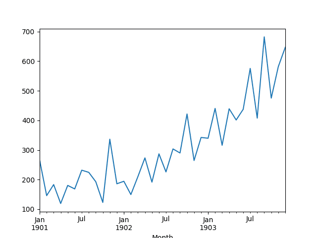
Shampoo Sales Dataset
Experimental Test Harness
Experiment: No Updates
Experiment: 2 Update Epochs
Experiment: 5 Update Epochs
Experiment: 10 Update Epochs
Experiment: 20 Update Epochs
Experiment: 50 Update Epochs
Comparison of Results
Environment
This tutorial assumes you have a Python SciPy environment installed. You can use either Python 2 or 3 with this example.
This tutorial assumes you have Keras v2.0 or higher installed with either the TensorFlow or Theano backend.
This tutorial also assumes you have scikit-learn, Pandas, NumPy, and Matplotlib installed.
If you need help setting up your Python environment, see this post:
Running the example loads the dataset as a Pandas Series and prints the first 5 rows.
1
2
3
4
5
6
7
Month
1901-01-01 266.0
1901-02-01 145.9
1901-03-01 183.1
1901-04-01 119.3
1901-05-01 180.3
Name: Sales, dtype: float64
A line plot of the series is then created showing a clear increasing trend.
Line Plot of Shampoo Sales Dataset
Next, we will take a look at the LSTM configuration and test harness used in the experiment.
Need help with Deep Learning for Time Series?
Take my free 7-day email crash course now (with sample code).
Click to sign-up and also get a free PDF Ebook version of the course.
Experimental Test Harness
This section describes the test harness used in this tutorial.
Data Split
We will split the Shampoo Sales dataset into two parts: a training and a test set.
The first two years of data will be taken for the training dataset and the remaining one year of data will be used for the test set.
Models will be developed using the training dataset and will make predictions on the test dataset.
The persistence forecast (naive forecast) on the test dataset achieves an error of 136.761 monthly shampoo sales. This provides an acceptable lower bound of performance on the test set.
Model Evaluation
A rolling-forecast scenario will be used, also called walk-forward model validation.
Each time step of the test dataset will be walked one at a time. A model will be used to make a forecast for the time step, then the actual expected value from the test set will be taken and made available to the model for the forecast on the next time step.
This mimics a real-world scenario where new Shampoo Sales observations would be available each month and used in the forecasting of the following month.
This will be simulated by the structure of the train and test datasets.
All forecasts on the test dataset will be collected and an error score calculated to summarize the skill of the model. The root mean squared error (RMSE) will be used as it punishes large errors and results in a score that is in the same units as the forecast data, namely monthly shampoo sales.
Data Preparation
Before we can fit an LSTM model to the dataset, we must transform the data.
The following three data transforms are performed on the dataset prior to fitting a model and making a forecast.
Transform the time series data so that it is stationary. Specifically, a lag=1 differencing to remove the increasing trend in the data.
Transform the time series into a supervised learning problem. Specifically, the organization of data into input and output patterns where the observation at the previous time step is used as an input to forecast the observation at the current time step
Transform the observations to have a specific scale. Specifically, to rescale the data to values between -1 and 1 to meet the default hyperbolic tangent activation function of the LSTM model.
These transforms are inverted on forecasts to return them into their original scale before calculating an error score.
LSTM Model
We will use an LSTM model with 1 neuron fit for 500 epochs.
A batch size of 1 is required as we will be using walk-forward validation and making one-step forecasts for each of the final 12 months of data.
A batch size of 1 means that the model will be fit using online training (as opposed to batch training or mini-batch training). As a result, it is expected that the model fit will have some variance.
Ideally, more training epochs would be used (such as 1000 or 1500), but this was truncated to 500 to keep run times reasonable.
The model will be fit using the efficient ADAM optimization algorithm and the mean squared error loss function.
Experimental Runs
Each experimental scenario will be run 10 times.
The reason for this is that the random initial conditions for an LSTM network can result in very different performance each time a given configuration is trained.
Let’s dive into the experiments.
Experiment: No Updates
In this first experiment, we will evaluate an LSTM trained once and reused to make a forecast for each time step.
We will call this the ‘no updates model‘ or the ‘fixed model‘ as no updates will be made once the model is first fit on the training data. This provides a baseline of performance that we would expect experiments that make modest updates to the model to outperform.
The complete code listing is provided below.
1
2
3
4
5
6
7
8
9
10
11
12
13
14
15
16
17
18
19
20
21
22
23
24
25
26
27
28
29
30
31
32
33
34
35
36
37
38
39
40
41
42
43
44
45
46
47
48
49
50
51
52
53
54
55
56
57
58
59
60
61
62
63
64
65
66
67
68
69
70
71
72
73
74
75
76
77
78
79
80
81
82
83
84
85
86
87
88
89
90
91
92
93
94
95
96
97
98
99
100
101
102
103
104
105
106
107
108
109
110
111
112
113
114
115
116
117
118
119
120
121
122
123
124
125
126
127
128
129
130
131
from pandas import DataFrame
from pandas import Series
from pandas import concat
from pandas import read_csv
from pandas import datetime
from sklearn.metrics import mean_squared_error
from sklearn.preprocessing import MinMaxScaler
from keras.models import Sequential
from keras.layers import Dense
from keras.layers import LSTM
from math import sqrt
import matplotlib
import numpy
from numpy import concatenate
# date-time parsing function for loading the dataset
def parser(x):
returndatetime.strptime('190'+x,'%Y-%m')
# frame a sequence as a supervised learning problem
Running the example stores the RMSE scores calculated on the test dataset using walk-forward validation. These are stored in a file called experiment_fixed.csv for later analysis. A summary of the scores is printed, shown below.
Note: Your results may vary given the stochastic nature of the algorithm or evaluation procedure, or differences in numerical precision. Consider running the example a few times and compare the average outcome.
The results suggest an average performance that outperforms the persistence model showing a test RMSE of 109.565465 compared to 136.761 monthly shampoo sales for persistence.
1
2
3
4
5
6
7
8
9
results
count 10.000000
mean 109.565465
std 14.329646
min 95.357198
25% 99.870983
50% 104.864387
75% 113.553952
max 138.261929
Next, we will start looking at configurations that make updates to the model during the walk-forward validation.
Experiment: 2 Update Epochs
In this experiment, we fit the model on all of the training data, then update the model after each forecast during the walk-forward validation.
Each test pattern used to elicit a forecast in the test dataset is then added to the training dataset and the model is updated.
In this case, the model is fit for an additional 2 training epochs before making the next forecast.
The same code listing as was used in the first experiment is used. The changes to the code listing are shown below.
Note: Your results may vary given the stochastic nature of the algorithm or evaluation procedure, or differences in numerical precision. Consider running the example a few times and compare the average outcome.
Running the experiment saves the final test RMSE scores in “experiment_update_2.csv” and prints summary statistics of the results, listed below.
1
2
3
4
5
6
7
8
9
results
count 10.000000
mean 99.566270
std 10.511337
min 87.771671
25% 93.925243
50% 97.903038
75% 101.213058
max 124.748746
Experiment: 5 Update Epochs
This experiments repeats the above update experiment and trains the model for an additional 5 epochs after each test pattern is added to the training dataset.
Note: Your results may vary given the stochastic nature of the algorithm or evaluation procedure, or differences in numerical precision. Consider running the example a few times and compare the average outcome.
Running the experiment saves the final test RMSE scores in “experiment_update_5.csv” and prints summary statistics of the results, listed below.
1
2
3
4
5
6
7
8
9
results
count 10.000000
mean 101.094469
std 9.422711
min 91.642706
25% 94.593701
50% 98.954743
75% 104.998420
max 123.651985
Experiment: 10 Update Epochs
This experiments repeats the above update experiment and trains the model for an additional 10 epochs after each test pattern is added to the training dataset.
Note: Your results may vary given the stochastic nature of the algorithm or evaluation procedure, or differences in numerical precision. Consider running the example a few times and compare the average outcome.
Running the experiment saves the final test RMSE scores in “experiment_update_10.csv” and prints summary statistics of the results, listed below.
1
2
3
4
5
6
7
8
9
results
count 10.000000
mean 108.806418
std 21.707665
min 92.161703
25% 94.872009
50% 99.652295
75% 112.607260
max 159.921749
Experiment: 20 Update Epochs
This experiments repeats the above update experiment and trains the model for an additional 20 epochs after each test pattern is added to the training dataset.
Note: Your results may vary given the stochastic nature of the algorithm or evaluation procedure, or differences in numerical precision. Consider running the example a few times and compare the average outcome.
Running the experiment saves the final test RMSE scores in “experiment_update_20.csv” and prints summary statistics of the results, listed below.
1
2
3
4
5
6
7
8
9
results
count 10.000000
mean 112.070895
std 16.631902
min 96.822760
25% 101.790705
50% 103.380896
75% 119.479211
max 140.828410
Experiment: 50 Update Epochs
This experiments repeats the above update experiment and trains the model for an additional 50 epochs after each test pattern is added to the training dataset.
Note: Your results may vary given the stochastic nature of the algorithm or evaluation procedure, or differences in numerical precision. Consider running the example a few times and compare the average outcome.
Running the experiment saves the final test RMSE scores in “experiment_update_50.csv” and prints summary statistics of the results, listed below.
1
2
3
4
5
6
7
8
9
results
count 10.000000
mean 110.721971
std 22.788192
min 93.362982
25% 96.833140
50% 98.411940
75% 123.793652
max 161.463289
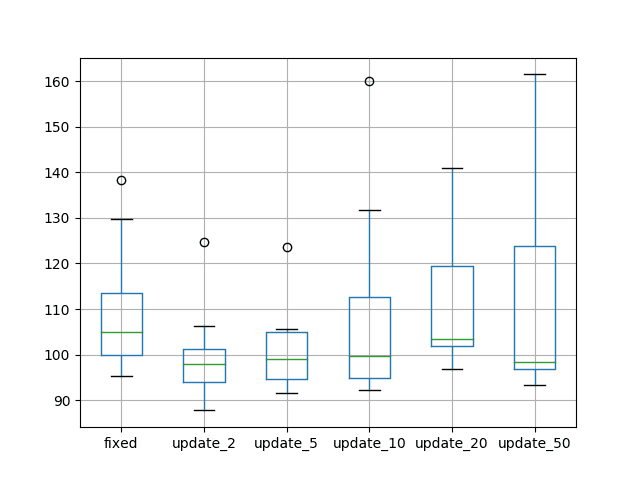
Comparison of Results
In this section, we compare the results saved from the previous experiments.
We load each of the saved results, summarize the results with descriptive statistics, and compare the results using box and whisker plots.
Running the example first calculates and prints descriptive statistics for each of the experimental results.
Note: Your results may vary given the stochastic nature of the algorithm or evaluation procedure, or differences in numerical precision. Consider running the example a few times and compare the average outcome.
If we look at the average performance, we can see that the fixed model provides a good baseline of performance, but we see that a modest number of update epochs (20 and 50) produce worse test set RMSE on average.
We see that a small number of update epochs result in better overall test set performance, specifically 2 epochs followed by 5 epochs. This is encouraging.
max 138.261929 124.748746 123.651985 159.921749 140.828410 161.463289
A box and whisker plot is also created that compares the distribution of test RMSE results from each experiment.
The plot highlights the median (green line) as well as the middle 50% of the data (box) for each experiment. The plot tells the same story as the average performance, suggesting that a small number of training epochs (2 or 5 epochs) result in the best overall test RMSE.
The plot shows a rise in test RMSE as the number of updates increases to 20 epochs, then back down again for 50 epochs. This might be a sign of significant further training improving the model (11 * 50 epochs) or an artifact of the small number of repeats (10).
Box and Whisker Plots Comparing the Number of Update Epochs
It is important to point out that these results are specific to the model configuration and this dataset.
It is hard to generalize these results beyond this specific example, although these experiments do provide a framework for performing similar experiments on your own predictive modeling problem.
Extensions
This section lists ideas for extensions to the experiments in this section.
Statistical Significance Tests. We could calculate pairwise statistical significance tests, such as the Student t-test, to see if the differences between the means in the populations of results are statistically significant or not.
More Repeats. We could increase the number of repeats from 10 to 30, 100, or more in an attempt to make the findings more robust.
More Epochs. The base LSTM model was only fit for 500 epochs with online training and it is believed that additional training epochs will result in a more accurate baseline model. The number of epochs was cut to decrease experiment run time.
Compare to more Epochs. The results for experiments that update the model should be compared directly to experiments of a fixed model that uses the same number of overall epochs to see if adding the additional test patterns to the training dataset makes any noticeable difference. For example, 2 update epochs for each test pattern could be compared to a fixed model trained for 500 + (12-1) * 2) or 522 epochs, an update model 5 compared to a fixed model fit for 500 + (12-1) * 5) or 555 epochs, and so on.
Completely New Model. Add an experiment where a new model is fit after each test pattern is added to the training dataset. This was attempted, but the extended run time prevented the results being collected prior to finalizing this tutorial. This would be expected to provide an interesting point of comparison to the update and fixed models.
Did you explore any of these extensions?
Report your results in the comments; I’d love to hear what you discovered.
Summary
In this tutorial, you discovered how to update an LSTM network as new data becomes available for time series forecasting in Python.
Specifically, you learned:
How to design a systematic set of experiments to explore the effect of updating LSTM models.
How to update an LSTM model as new data becomes available.
That updates to an LSTM model can result in a more effective predictive model, but careful calibration is required on your forecast problem.
Do you have any questions?
Ask your questions in the comments below and I will do my best to answer.
Develop Deep Learning models for Time Series Today!
The real question is under what circumstances should we use LSTMs over classical methods like ARIMA.
I hope to answer that in my new book. Generally, if you want to easily handle multivariate input, multi-step output, and non-linear relationships in the data.
Hi Jason,
Nice post. I am working on LSTM. I’d like add two layers for each variable with different weight. Is it possible?
Could you have me any heads up?
Sorry, I did not make my point.
Current, I have two input and I know that one of the input is more important than another. I’d like to give importance to it when training my model. For what I mean, I try to give each of the two input a different weight in order to make my forecasting more precise.
Is it possible?
Thank you for your time.
How is the learning rate factored in with each .fit ? My understanding was that it restarts with each each “update”, making online learning difficult in this case – is that correct?
(not saying anything is correct or incorrect, just trying to understand)
Is it possible to perform online training keeping the last state of the previous fitting (learning rate, momentum, etc)? I believe that could bring different results.
Thank you very much Jason. These LSTM posts are amazing!
I have one question about the update. Would it make a difference to make the update not using the entire training + last test_scaled[i, 0:-1], test_scaled[i, -1], but just a smaller part on the train and the slice? For example, 1/3 last training samples + test. What do you think?
Trying to understand your batch size of 1, i.e. “A batch size of 1 is required as we will be using walk-forward validation and making one-step forecasts … the model will be fit using online training (as opposed to batch training or mini-batch training).”
First, we’re doing two fits: An initial fit and then an update fit. Seems our batch size could be larger for the initial fit?
But second, even for that update fit, we’re not fitting just one observation alone, but rather refitting the entire training set + 1 more observation.
My dataset is 17,000 observations, making training time quite long. Just looking for ideas to speed it up.
When using a stateful LSTM we have to use the same batch size in Keras for fitting and predicting. It sucks. The requirement here to make one step (one batch) forecasts limits training.
However, when I try to run the update for the 2 epochs it seems to get stuck in an infinite loop. It doesn’t finish. Maybe there is a mistake in the update function? What do you think?
I am a newbie to Recurrent Neural Networks and have a naive question regarding the cell state updates in experiment 0:
You said that the model would not be updated once trained on the training set in expt. 0. To me, this means that none of the model parameters learnt after training lstm on training data (first 24 months) would be changed while making predictions for next 12 months. However, I am wondering whether the cell state of LSTM be also fixed or is allowed to be continuously updated as we encounter the data points in testing set? That is, while making prediction at the 30th month, would the cell state of LSTM be updated based on the inputs it received for 25th-29th months? Or would it be fixed to what was obtained after training LSTM on first 24 months?
My intuition says that it should be continuously updated as we receive the data points from testing set. However, I could not see it happening explicitly in the code, unless it happens internally in lstm model?
THe cell state is updated as we move through the data, but the cell state is also reset at the end of each batch, or explicitly when we all reset_states() on the model.
Hi Jason,
At time of updation of model, why it is required to reset the cell state? As per my understanding and intuition it should hold previous cell state for better efficiency in time series modelling.
Transform the observations to have a specific scale. Specifically, to rescale the data to values between -1 and 1 to meet the default hyperbolic tangent activation function of the LSTM model.
Is this always the case? If we opt to use Relu as the activation function, is it best practice to always keep the range of the series 0< ?
In some of your earlier posts (2017) with LSTM, you have scaled using MixMaxScaler between -1 and 1 and not given any activation in the first .fit line allowing the default Tahn activation
However, in other set of newer posts (early 2018 onwards), you have given activiation=relu in the first line of .fit command and not scaled the data.
Based on your comment above, do you recommend to use MixMaxScaler (0,1) and RELU together while fitting the model for an LSTM?
That makes sens, thank you! But just throwing it out there, shouldn’t it be the same number of iterations as the initial model? To keep things uniform?
Thank you for your continued reply. I am learning a lot.
One more question, if you don’t mind.
Am I wrong when I say that “the model learns the sequential dependencies and patterns of the test data set as it goes through the test data to predict when the model is stateful”?
So, in that sense, there is no need to update the model by refitting, since as it goes through each test step, it learns new patterns. Is that correct?
Hi Jason.
Is it possible that rather than training the lstm network all over again with all the previous data points, we can just fit the model to the new data point as well since for the above approach it is taking a very long time to retrain itself making it extremely slow for any real time work. It is taking hours for a dataset of around 1000 values even on a fairly powerful system.
But herein the entire LSTM is being trained all over again. But is there any way to simply fit the existing weights and model to the new data point only since that may be faster than to process al the datapoints again.
In real world, we cannot do difference, supervise conversion, scale for the new data, like test set of the example. Does it means that we have to keep the raw data and merge it with new data, and then repeat difference, supervise conversion and scale procedure every time slot?
If so, it costs a lot of resource of the system. If there is better way to update model with the new data without retraining everything.
Continue with Shampoo Sales example. After receiving the latest month data, if it could be used to fit model directly? It is a single value. Thereby difference and scale are not feasible.
model.fit(X, y, nb_epoch=1, batch_size=batch_size, verbose=0, shuffle=False)
Does it also mean model.reset_states() should not execute for the whole online training procedure, after the offline training?
Hi Jason — correct me if I’m wrong here (and also my apologies if you’ve answered this elsewhere), but are you resetting the state after every single batch (of size 1)? Doesn’t that mean we are more or less losing the effectiveness of the LSTM cell? We can’t learn anything about dynamics of anything earlier in time than time t-1 if we reset the state after only seeing one step…
Hello Jason, first of all Thanks for sharing your knowledge with all of us.
I already got trained model and want to re-train it, with new data, (data_original+data_new). Problem is, if I load the model and want to continue in training, it seems to start from scratch. This happens even when I use exactly the same setup and data, which were used for training original model. Could you please give me a hint what I am doing wrong?
def update_model(model, train, batch_size, updates):
X, y = train[:, :-n_seq], train[:, -n_seq:]
X = X.reshape(X.shape[0], n_lag, n_features)
for i in range(updates):
model.fit(X, y, nb_epoch=1, batch_size=batch_size, verbose=0, shuffle=False)
model.reset_states()
return model
model = load_model(“multivariete_model.h5”)
update_model(model, train, 1, updates)
Hi, Jason, I have some questions about online learning of LSTM network for time series forecasting.
Considering the time cost due to LSTM network training, we hope to retrain the previous model when processing the next time point data.
So, we need to do two fits: an initial fit and then an update fit.
For the initial fit, we choose a larger batch-size for the stateless LSTM network. And for the update fit, we choose batch-size=1 for retraining the model based on the initial fit.
Is there any problem with this idea?
I would also like to ask you very much. I am a rookie in machine learning. Only update tne model for the new data (online-learning). Is there any way to program it??
just on a quick note: you write “Statistical Significance Tests. We could calculate pairwise statistical significance tests, such as the Student t-test, to see if the differences between the means in the populations of results are statistically significant or not.”
One would probably test the significance of differences between the means by performing an Anova, I guess?
Hi Jason,
How can i make an LSTM model work if I dont have a large training dataset? Moreover, if the time series data is updating as lets say – the data i am tracking gets updated once in a month and I get a single new data point in a month , in order to predict one step ahead of it , I need to train the model with the new data point again?
“For example, 2 update epochs for each test pattern could be compared to a fixed model trained for 500 + (12-1) * 2) or 522 epochs, an update model 5 compared to a fixed model fit for 500 + (12-1) * 5) or 555 epochs, and so on.”
From the above example what is 12?
Say I have 10 days of data. Each day has 375 rows.
For the first model, I run 100 epochs and subsequent fits of 9 model I select 2 epochs. Then for Model 2 total epochs would be
Hey Jason,
This is a great work! I really learned a lot from your post. Thank you very much.
However, I a, wondering if you have tried to forecast your test data by using the predicted values instead of the available test data?
In other word, in “Experiment: 2 Update Epochs/ Forecast test dataset section in line 35, you use the test data to predict next time step.that is okay for initializing the forecasting, but my question is why you do not use the predicted values that generated from previews prediction step to update the model and make forecasting for next time step? I think that is more realistic.
I think this post is different than what I asked about.
My question is especially about line 35 in Experiment: 2 Update Epochs/ Forecast test dataset section where you used the available test data to update the model and make new prediction.
My question is why you did not use the prediction value to update the model(retrain it) and later compare the forecast test with the real test data? (just assume you do not have the test data and make prediction then compare with the available test data)
I am asking this because I want to see if there is way to make prediction for 10 or 20 time step ahead and that is what most investors would like to see before making any big decision!
What do you think is the best way to deal with that?
Again, the goal of my question is to learn NOT to criticize your work!
Thank you for the nice tutorial. I am new to RNNs, and here’s the (possibly dumb) question that I have:
If the aim is to train an LSTM in an incremental fashion, why do we need training data? Can’t we just start from complete cold-start and incrementally train the model one observation at a time, using the prediction for the next time step for evaluation (I think this is called prequential evaluation)?
What I meant was evaluating and training the model in purely online, reinforcement learning-type of setting. The training data would be revealed one data point at a time. The next data point is used as the ground truth for prediction, and then fed into the algorithm for an incremental update. So you basically start with no data, and there is no train-test split. Do you think an RNN can be trained in that way?
It can be done, it is called online learning, but is not common with deep learning, that requires the opposite – lots of data and training prior to use.
a few points about online learning from scratch:
– if you have no historical data, at what point in time will you be able to trust the prediction? How will you know when you arrive at success?
– in order to tune your model you need to alliteratively retrain with different parameters. this can’t be done with no data, so really you have to wait until some point in the future when you have accumulated enough data to re-run through tests with different settings, and run statistics on the results to find the best tuned model. so really online from scratch doesn’t exist!
It would not be appropriate to scale the series after it has been transformed into a supervised learning problem as each column would be handled differently, which would be incorrect.
But why do you scale data after it has been transformed into a supervised learning problem in the code of this post?
I have some simple questions;
I am using LSTM to predict load forecast or 1 day (24 values ahead).
After trying to predict only 1 value and append it to history and predict the following 23 values same way (result is not good), i now want to use dense(24), predicting at once 24 points.
(Input 24×10 for example, output 24 Outputs at once).
I tried for example splitting my input and output data in this method; for example 10 days before and the output is 1 day.
The tesult is a shape of middle line (does not follow the real data), not good.. (maybe needs more epochs.. but now i had a new idea:
Is it possible to split the Inputs so that the next sample is not not t+1, but t+24 (next day)?? Or Am i doing something wrong here?
That means i want to try: t-24, t-48, t-72, …… so the model sees exactly 1 day shifts.
Am i transgressing a rule?
Second question:
Another case:
For my Cross-validation, i did this:
Using a function i created to do incremental learning following this loop:
(train from day 1 to 19-> predict day20 -> refit again the model using the real data for the next train (true data of the prediction day20-> predict day 21-> train using real day21-> predict day22 -> train using real day22-> predict day23 etc…)
the model somehow forgets everything after refitting it one more time and gives me an output nearly the same as last train day..
(predicted day 21 ist same as train day 20)
(predicted day 22 ist same as train day 21)
(predicted day 23 ist same as train day 22)
…
Does fitting an LSTM model again let it forget everything it has learned from previous fits?
If then, how can i do incremental learning for my cross validation?
yes, i need 24 for multi-step forecasting, but i am talking about the time shift between samples, can it also be 24 time steps shift (normally it is 1 time step shift in LSTM (t-4, t-3, t-2, t-1 ..))??
so can it be (…. , t-72, t-48, t-24)?
Hi, I am trying to teach an LSTM network a very basic substitution rule, lets say replace:
a =>x
b =>y
c => w
I am using this character level architecture https://github.com/tensorflow/tfjs-examples/tree/master/translation which uses an LSTM but unfortunately even if I get very lost function i.e. less than1e-6, I am getting very poor results on the predictions. For this toy experiment, the output length should be always the same as the input length, like:
abc => xyw
But LSTM some times gives extra characters is this the nature of the LSTM?
Hello Sir, I have implemented the codes from https://www.kaggle.com/eray1yildiz/using-lstms-with-attention-for-emotion-recognition/comments. I have already train the model and I am doing the prediction part. From this implementation, the guy used a sample text to predict the emotion, but me I want to use a dataset containg a dataframe of comment and I want the system to predict the result for each comment as well as creating a new column in the dataframe so as to input the predicted result in each row for their respective comments. Can you help me on how to do that? Please sir.
\you can mail me if possible so that I can show you how my dataframe is and what output I am willing to get,.
Thank you so much. I would be grateful if you could help me. Thank you sir.
I’m trying to execute the “Experiment: No Updates” code mentioned above. However, getting the error “ValueError: setting an array element with a sequence.” on the line “results[‘results’] = experiment(repeats, series)”.
Please help me to solve this.
Thanks in advance
Nice, self explanatory. I wonder to ask how would you create you neural network if would like to train model with first six month, and “update-train” model with 12-18months data. Is it even possible?
I would encourage you to test a suite of different models and different data preparation methods and discover what works best for the prediction problem.
hi,
thanks for ur rply. you have mentioned batch size 1 in the initial fit this makes the training time more. i need to get one step prediction can i increase the batch size for intial fit
Hi, first of all I’d like to thank you for your tutorials.
However I have a question. I want to use LSTM for anomaly detection on not labelled time series data. What approach would you recommend me? Currently I’m trying to use similar approach as I used with other models (ARIMA and smoothing) – create a rolling forecast of the data (using the method suggested in this tutorial), calculate differences between actuals and predictions. Calculate moving average of the differences and label as a anomaly all distances with difference larger than the corresponding moving average value plus some multiple of standard deviation. Is this a good way to go?
Thanks in advance for your reply.
André de Sousa AraujoSeptember 6, 2020 at 5:03 am#
Hi jason,
I got this error:
– TypeError: fit() got an unexpected keyword argument ‘nb_epoch’
It’s just epochs now. nb_epoch was deprecated. I have changed and then work form me!
Thanks
André
hi Jason,
For the part ,where model is not fixed, and we are updating it , i have 2 questions.
1. RMSE over every next attempt should be going down, which is not the case , rather it is randomly fluctuating.
2.when we are updating 50 times as compared to 2 times, how come the results are deteriorating .? At best they should not improve.
Correct me if I’m wrong, but if I’m trying to predict a multi-step output (say 7 days), and after every prediction of a datapoint in the test set, I update the model with that datapoint, am I not leaking data? When I update the model, I know the actual target value on day 1, but the target values days 2 – 6 are not known to me, and yet I would still be updating the model with the actual target values of days 2 – 6. Am I misunderstanding something? How should I go about dealing with this problem?
Since the output has to always be of the same length, the only solution I can think of is to take the prediction for the 7 days, substitute the first value with the actual value, and then train on it. However, this seems like a terrible idea, since I’ll be training on almost-certainly incorrect data for days 2 – 6.
As long as you don’t use the future to predict the past, you’re fine. And you can use predictions about the future as input to predict subsequent time steps if you want – e.g. a recursive forecasting model.
Thank you so much! That post was extremely helpful.
I went ahead and implemented the models in that post, except the last one (at least so far). I’ve been playing around with them for a few days, and I have a few questions.
1) I’m working on weather-like data, that is a mostly a function of non-linear interactions between the independent variables from the prior two weeks, and the data should also look somewhat similar to the same data from a year prior. Because of the non-linearities, I am not using a model like ARIMA. Are there any parameters that I should consider passing to the layers of the LSTM that would account for data being similar to that of a year prior? I already have dummy variables for the period of the year + cross terms. I looked through the documentation for Keras LSTM but didn’t find anything obvious.
2) I’m not sure that I understand why the model isn’t leaking. Once I started that walk-forward validation + update model strategy using XGBRegressor for feature selection + FNN when I was implementing it, the results were getting so good that I was sure that I was leaking data, which is why I switched to LSTM. Once I implemented walk-forward validation + update model in the LSTM setting, the results were really, really good.
I confused by the fact that if I wanted to make real-time predictions with this model, I wouldn’t actually have the ability to use the most up-to-date sequences of target variables to update my model. For example, if I’m trying to predict the next 30 days, in real life, the only accurate data I would be to use to update the model are the datapoints from 30 days ago. I have implemented both the lag version and the up-to-date version, and naturally, the latter gives much better results, which leads me to want to understand why the model isn’t leaking data. Is there some deeper intuition to the matter, or does it basically boil down to, as you said, “As long as you don’t use the future to predict the past, you’re fine”?
3) Another question I have regards the results of trying to predict a sequence of the differences of the target variable (as you described in that post I mentioned), instead of a sequence of the target variables. I’m experiencing a few unusual problems:
3a) If I add the target variable on the current day t_c to each of the differences at d_{c+1}, d_{c+2}, …, individually, i.e. my predictions are t_c + d_{c+1}, t_c + d_{c+2}, …, I get much better results than when I take the rolling sum over the differences, i.e. when my predictions are t_c + d_{c+1}, t_c + d_{c+1} + d_{c+2}, …. This seems to imply that the model is learning to predict changes relative to t_c, rather than the difference between t_{c + k} and t_{c + k + 1}, k > 0. I have verified this with manual inspection, and that does seem to be what’s happening. I’ve made sure that I’ve looking at the differences between consecutive days, and not the difference between t_c and t_{c + k}, k > 1. I’m not sure what to make of this.
3b) Under most combinations of parameters, the predicted differences are either all positive, or all negative, and usually don’t vary much over the prediction period (30 days). In most cases where there is a mixture, the differences are all around zero anyway. It seems like the model isn’t willing to “take risks”, so to speak. I have tried changing the learning rate to fix this, but can’t think of much else.
3c) When I do the walk-forward validation + update on the differences, the results get much worse, the exact opposite of the case when I’m predicting the variables directly, without differencing.
3d) Scaling seems to have a bad effect on the differencing model, either for feature_range=(0, 1) or feature_range=(-1, 1). The difference between days is almost always between -1 and 1 anyway.
For all of these models, it seems like training for more than about three epochs leads to serious overfitting, except in the case of the walk-forward validation + update model strategy, where +/- 15 seems about optimal.
Sorry for the lengthy questions. I’m happy to read any material you think is relevant, I understand that I asked a lot.
Yeah, sorry about that, I was working through some of issues with this problem I’m trying to solve. For anyone who happens to stumble on this comment and is wondering how I resolved it:
The solution mentioned their uses some kind of attention mechanism. For my purposes, I opted for a simpler version, and ended up just retraining on the same time slice of the prior year. Although I find the concept described there interesting and would like to try it in the future.
2) I misinterpreted Jason’s first response to my question – I thought the implication was that what I was describing was not leaking data, which is why I got confused. If I’m understanding correctly, the model I described was, in fact, leaking data. Suppose you want to predict the next week of data, for every day some time period, say a month. Today is day 1, and you predict days 2 – 8. The next prediction to make would be having the data from day 1, today being day 2, and you predicting days 3 – 9. After the first prediction on day 1, when you predict days 2 – 8, you cannot then train on the correct data for days 2 – 8. You must wait at least until you are on day 8, trying to predict days 9 – 15, to update your model with the data from day 1, when you were trying to predict days 2 – 8.
3) Differencing is usually used to make non-stationary data stationary. This wasn’t the case with my data, although I’m not sure that addresses all of the issues I mentioned.
Hi Jason, can I ask is there a reason as to why the number of neuron is set to one is this sample. I understand that a batch-size of 1 is so that new data can be instantly refitted to the model but can I change the neuron to 10/20/50 or is a neuron of 1 is a must in walk-forward validation for LSTM?
Hi Jason Brownlee,
the knowledge you shared are excellent. An example to be followed by everyone because it is the only way to move forward. I’ll test it on the problem I’m trying to solve. Thanks
Hello, Adrian Tam, your article is very helpful to me.
As a novice, I don’t understand why the function update_ Model() does not need to take the model as the return value? Will the model inherit the updated content? I hope you can explain it in detail. Thank you very much!
Because the model is an object created outside of the function and in the function, we just mutate it. In other programming languages, we call this “pass-by-reference”.
I have one more question regarding the updating process. While testing are we taking the actual values from the test data in the current time step for predicting the next time step or are we taking the predicted values and adding them to the list for the prediction of the future time step ?
In what we can we take actual values from the test set and make a prediction based on them?
Hi Sapna…Predicted values are being added to a “history” that is used to make further predictions. Considerable more detail can be found in the following resource:
Thank you for your response. I have a battery dataset with cycle and capacity values. I want that when I train it on 100 cycles, for the testing process, it should take the actual value of capacity at 101th cycle and then predict the capacity for 102th cycle. So how can I provide actual value to the model rather than the predicted values for future predictions?
I want to update the model after it has made predictions on the 3 months of the test set so rather than updating after each month’s prediction I want the model to update after some time to save the number of times the model is getting retrained.
Hi Jennifer…How is your model progressing? Let us know if we can help answer any questions regarding the tutorial. You may also wish to consider hybrid CNN-LSTM models.


Hey Jason,
Your tutorials and experiments are to the point and well explained. Thanks for sharing and Keep up the good work.
Thanks Rohit.
A bit off-topic. Does LSTM perform better than the usual time series methods or machine learning methods?
Ouch. It depends, like any algorithm.
See the no free lunch theorem:
https://en.wikipedia.org/wiki/No_free_lunch_in_search_and_optimization
The real question is under what circumstances should we use LSTMs over classical methods like ARIMA.
I hope to answer that in my new book. Generally, if you want to easily handle multivariate input, multi-step output, and non-linear relationships in the data.
Hi Jason,
Nice post. I am working on LSTM. I’d like add two layers for each variable with different weight. Is it possible?
Could you have me any heads up?
Sorry, not sure what you mean two layers for each variable with different weight.
Perhaps you could elaborate?
Sorry, I did not make my point.
Current, I have two input and I know that one of the input is more important than another. I’d like to give importance to it when training my model. For what I mean, I try to give each of the two input a different weight in order to make my forecasting more precise.
Is it possible?
Thank you for your time.
Generally, no. We prefer to let the algorithm learn the importance of the inputs.
Thank you for your advice. Got it.
Hi. Very interesting subject. Thank you.
What do mean by update 2, 20, 50 epoch?
Changing the number of training epochs.
Very nice post Thank you Jason
I’m glad you found it useful.
Hey Jason, that’s really an interesting post.
By the way, during experiment 2, row 24, you use an update_model never defined before.
Cheers,
Cristian
Opps, sorry. I’ve added the missing function. Thanks.
Hi Jason,
I noticed that update_model function is not defined, do you mind adding it to the listings?
Thanks, I’ve added the function.
It is indeed a nice post. But how do you generate forward forecast using LSTM here?
What do you mean exactly?
Finalize your model and call model.predict().
heartfelt gratitude to this excellent post!
I’m glad you found it useful Sam, thanks.
How is the learning rate factored in with each .fit ? My understanding was that it restarts with each each “update”, making online learning difficult in this case – is that correct?
(not saying anything is correct or incorrect, just trying to understand)
In this case we use Adam where each “parameter” (weight) has its own learning rate. See here:
https://keras.io/optimizers/#adam
And it preserves the decay / rate for each weight from the previous “update”?
Hi Jason, very interesting! Thanks!
Is it possible to perform online training keeping the last state of the previous fitting (learning rate, momentum, etc)? I believe that could bring different results.
David
You’re welcome!
You can keep the last state. Not sure about the state of the SGD. It may not be worth it. Perhaps experiment and see if it helps.
Thank you very much Jason. These LSTM posts are amazing!
I have one question about the update. Would it make a difference to make the update not using the entire training + last test_scaled[i, 0:-1], test_scaled[i, -1], but just a smaller part on the train and the slice? For example, 1/3 last training samples + test. What do you think?
It may. Try it and report what you get.
Trying to understand your batch size of 1, i.e. “A batch size of 1 is required as we will be using walk-forward validation and making one-step forecasts … the model will be fit using online training (as opposed to batch training or mini-batch training).”
First, we’re doing two fits: An initial fit and then an update fit. Seems our batch size could be larger for the initial fit?
But second, even for that update fit, we’re not fitting just one observation alone, but rather refitting the entire training set + 1 more observation.
My dataset is 17,000 observations, making training time quite long. Just looking for ideas to speed it up.
Hi Kim.
When using a stateful LSTM we have to use the same batch size in Keras for fitting and predicting. It sucks. The requirement here to make one step (one batch) forecasts limits training.
I have a workaround though, see this:
https://machinelearningmastery.com/use-different-batch-sizes-training-predicting-python-keras/
Or just don’t make the LSTM stateful.
Jason, thank you for the continued flow of relevant content. I’ll post an additional tip I learned over on your referenced blog.
I’m here to help if I can Kim.
Hi Jason,
Wonderful post.
However, when I try to run the update for the 2 epochs it seems to get stuck in an infinite loop. It doesn’t finish. Maybe there is a mistake in the update function? What do you think?
Perhaps reduce the amount of data and see if it makes a difference – it could be a machine speed or RAM thing?
Hi Jason,
Thanks for the wonderful post.
I am a newbie to Recurrent Neural Networks and have a naive question regarding the cell state updates in experiment 0:
You said that the model would not be updated once trained on the training set in expt. 0. To me, this means that none of the model parameters learnt after training lstm on training data (first 24 months) would be changed while making predictions for next 12 months. However, I am wondering whether the cell state of LSTM be also fixed or is allowed to be continuously updated as we encounter the data points in testing set? That is, while making prediction at the 30th month, would the cell state of LSTM be updated based on the inputs it received for 25th-29th months? Or would it be fixed to what was obtained after training LSTM on first 24 months?
My intuition says that it should be continuously updated as we receive the data points from testing set. However, I could not see it happening explicitly in the code, unless it happens internally in lstm model?
THe cell state is updated as we move through the data, but the cell state is also reset at the end of each batch, or explicitly when we all reset_states() on the model.
How i retrain my model with new dataset .and append the result with previous result?
Does the above post help?
Hi Jason,
At time of updation of model, why it is required to reset the cell state? As per my understanding and intuition it should hold previous cell state for better efficiency in time series modelling.
Generally, the end of a sample or end of batch is a good time to clear state as it is often not relevant to the next sample or state.
If it is, don’t reset the state.
Experiment and see what works best for your data.
Hi Jason,
In your statement:
Transform the observations to have a specific scale. Specifically, to rescale the data to values between -1 and 1 to meet the default hyperbolic tangent activation function of the LSTM model.
Is this always the case? If we opt to use Relu as the activation function, is it best practice to always keep the range of the series 0< ?
Thanks!
No, today I would recommend rescaling data to 0-1 for LSTMs.
I also do not recommend changing the transfer functions within LSTM units.
Hi Jason,
In some of your earlier posts (2017) with LSTM, you have scaled using MixMaxScaler between -1 and 1 and not given any activation in the first .fit line allowing the default Tahn activation
However, in other set of newer posts (early 2018 onwards), you have given activiation=relu in the first line of .fit command and not scaled the data.
Based on your comment above, do you recommend to use MixMaxScaler (0,1) and RELU together while fitting the model for an LSTM?
Yes, scaling the data caused more confusion to readers than I would have liked.
Relu makes the model less sensitive to data scale.
I still recommend scaling data, test with and without, more here:
https://machinelearningmastery.com/how-to-improve-neural-network-stability-and-modeling-performance-with-data-scaling/
Hi Jason,
What is the reason behind multiple updates?
“In this case, the model is fit for an additional 2 training epochs before making the next forecast.”
It doesn’t make sense to me. Shouldn’t it only be 1 training epoch, for the “next-time step”?
Thanks!
Learning in neural networks is an iterative process of reducing error. We cannot know the right number of iterations other than by testing.
That makes sens, thank you! But just throwing it out there, shouldn’t it be the same number of iterations as the initial model? To keep things uniform?
where updates is actually nb_epochs in your fit_lstm().
Not if we are using the trained weights as a starting point. Something has already been learned and we are refining it.
That being said, always test updated models vs new models.
Thank you for your continued reply. I am learning a lot.
One more question, if you don’t mind.
Am I wrong when I say that “the model learns the sequential dependencies and patterns of the test data set as it goes through the test data to predict when the model is stateful”?
It does this for stateful and stateless models.
The difference is that stateful models give you control over when internal state is reset.
So, in that sense, there is no need to update the model by refitting, since as it goes through each test step, it learns new patterns. Is that correct?
No, updating refers to updating the model weights.
Think of the internal state as variables that the model can use as it is making predictions.
Hi Jason.
Is it possible that rather than training the lstm network all over again with all the previous data points, we can just fit the model to the new data point as well since for the above approach it is taking a very long time to retrain itself making it extremely slow for any real time work. It is taking hours for a dataset of around 1000 values even on a fairly powerful system.
Sure, try many approaches and see what works best for your specific data and project requirements.
But herein the entire LSTM is being trained all over again. But is there any way to simply fit the existing weights and model to the new data point only since that may be faster than to process al the datapoints again.
We are only updating the existing weights each time.
ok.glad to hear that.
Thanks a lot once again Jason.
🙂
Hi Jason,
Thanks a lot for providing the link of this page.
In real world, we cannot do difference, supervise conversion, scale for the new data, like test set of the example. Does it means that we have to keep the raw data and merge it with new data, and then repeat difference, supervise conversion and scale procedure every time slot?
If so, it costs a lot of resource of the system. If there is better way to update model with the new data without retraining everything.
You do not need to rebuild the whole model, you can refit only on new/recent data.
Thanks for replying, Jason.
Continue with Shampoo Sales example. After receiving the latest month data, if it could be used to fit model directly? It is a single value. Thereby difference and scale are not feasible.
model.fit(X, y, nb_epoch=1, batch_size=batch_size, verbose=0, shuffle=False)
Does it also mean model.reset_states() should not execute for the whole online training procedure, after the offline training?
Why? The prior ob is required to difference, and the min/max can be estimated from training data.
Resetting state may or may not impact the model. It is worth testing whether warming up internal state matters or not for a given problem.
Hi Jason — correct me if I’m wrong here (and also my apologies if you’ve answered this elsewhere), but are you resetting the state after every single batch (of size 1)? Doesn’t that mean we are more or less losing the effectiveness of the LSTM cell? We can’t learn anything about dynamics of anything earlier in time than time t-1 if we reset the state after only seeing one step…
Thanks for the post!
Yes, mostly, we loose BPTT, but the LSTM still has memory across the samples.
Hello Jason, first of all Thanks for sharing your knowledge with all of us.
I already got trained model and want to re-train it, with new data, (data_original+data_new). Problem is, if I load the model and want to continue in training, it seems to start from scratch. This happens even when I use exactly the same setup and data, which were used for training original model. Could you please give me a hint what I am doing wrong?
def update_model(model, train, batch_size, updates):
X, y = train[:, :-n_seq], train[:, -n_seq:]
X = X.reshape(X.shape[0], n_lag, n_features)
for i in range(updates):
model.fit(X, y, nb_epoch=1, batch_size=batch_size, verbose=0, shuffle=False)
model.reset_states()
return model
model = load_model(“multivariete_model.h5”)
update_model(model, train, 1, updates)
You must save the weights to file, then later you can reload them and continue training.
Can we apply Grid search method for hyperparameter optimization in LSTM model?
Yes, see this post:
https://machinelearningmastery.com/tune-lstm-hyperparameters-keras-time-series-forecasting/
Hi, Jason, I have some questions about online learning of LSTM network for time series forecasting.
Considering the time cost due to LSTM network training, we hope to retrain the previous model when processing the next time point data.
So, we need to do two fits: an initial fit and then an update fit.
For the initial fit, we choose a larger batch-size for the stateless LSTM network. And for the update fit, we choose batch-size=1 for retraining the model based on the initial fit.
Is there any problem with this idea?
I recommend testing and use model performance to guide whether it is a good idea or not.
I would also like to ask you very much. I am a rookie in machine learning. Only update tne model for the new data (online-learning). Is there any way to program it??
Yes, call model.fit() with new data.
Hi Jason,
I am not sure why I keep getting the following error when executing the Experiment: No update.
127 results = DataFrame()
128 # run experiment
–> 129 results[‘results’] = experiment(repeats, series)
130 # summarize results
131 print(results.describe())
AttributeError: ‘NoneType’ object has no attribute ‘values’.
This code is the same as the one in https://machinelearningmastery.com/multi-step-time-series-forecasting-long-short-term-memory-networks-python/ which just worked perfectly when I tried to follow the post in its entirety.
I restarted the kernel for Update LSTM experiment no update many times… still not helping…
Thanks in advance!
I have some suggestions here:
https://machinelearningmastery.com/faq/single-faq/why-does-the-code-in-the-tutorial-not-work-for-me
Hi Jason,
just on a quick note: you write “Statistical Significance Tests. We could calculate pairwise statistical significance tests, such as the Student t-test, to see if the differences between the means in the populations of results are statistically significant or not.”
One would probably test the significance of differences between the means by performing an Anova, I guess?
Best
No, Student’s t-test would be more appropriate, the paired version if the same data is used.
More advanced approaches here:
https://machinelearningmastery.com/statistical-significance-tests-for-comparing-machine-learning-algorithms/
Hi Jason,
I think this is not revelant to this topic, Sorry!
But anyways I wanted to know if you have a post explaining about incremental sequence learning?
Thanks!
Do you mean updating models?
https://machinelearningmastery.com/update-lstm-networks-training-time-series-forecasting/
Hi jason,
is it possible to train lstm with swarm intelligence algorithms such as aco and pso ?
Perhaps, but I would expect it to be less efficient than SGD.
Hi Jason,
How can i make an LSTM model work if I dont have a large training dataset? Moreover, if the time series data is updating as lets say – the data i am tracking gets updated once in a month and I get a single new data point in a month , in order to predict one step ahead of it , I need to train the model with the new data point again?
Perhaps start with a linear model, and adopt an LSTM only if it outperforms the linear model:
https://machinelearningmastery.com/how-to-develop-a-skilful-time-series-forecasting-model/
hi Jason ,
How de we make prediction for future values ?
Good question, I answer it here:
https://machinelearningmastery.com/make-predictions-long-short-term-memory-models-keras/
Hi Jason,
“For example, 2 update epochs for each test pattern could be compared to a fixed model trained for 500 + (12-1) * 2) or 522 epochs, an update model 5 compared to a fixed model fit for 500 + (12-1) * 5) or 555 epochs, and so on.”
From the above example what is 12?
Say I have 10 days of data. Each day has 375 rows.
For the first model, I run 100 epochs and subsequent fits of 9 model I select 2 epochs. Then for Model 2 total epochs would be
100 + (375-1)*2?
Hey Jason,
This is a great work! I really learned a lot from your post. Thank you very much.
However, I a, wondering if you have tried to forecast your test data by using the predicted values instead of the available test data?
In other word, in “Experiment: 2 Update Epochs/ Forecast test dataset section in line 35, you use the test data to predict next time step.that is okay for initializing the forecasting, but my question is why you do not use the predicted values that generated from previews prediction step to update the model and make forecasting for next time step? I think that is more realistic.
This post may help you to make a forecast:
https://machinelearningmastery.com/make-predictions-long-short-term-memory-models-keras/
I think this post is different than what I asked about.
My question is especially about line 35 in Experiment: 2 Update Epochs/ Forecast test dataset section where you used the available test data to update the model and make new prediction.
My question is why you did not use the prediction value to update the model(retrain it) and later compare the forecast test with the real test data? (just assume you do not have the test data and make prediction then compare with the available test data)
I am asking this because I want to see if there is way to make prediction for 10 or 20 time step ahead and that is what most investors would like to see before making any big decision!
What do you think is the best way to deal with that?
Again, the goal of my question is to learn NOT to criticize your work!
I’m looking forward to your feedback
Thank you
Perhgaps because I was demonstrating how to update models, that is the focus of the post. It was years ago.
Im sure you get this question asked a lot, but I must know. Are you related to Marquees Brownlee?
First time I’ve been asked 🙂
We’re not directly related as far as I know.
And he is way more famous:
https://en.wikipedia.org/wiki/Marques_Brownlee
Hi Jason,
Thank you for the nice tutorial. I am new to RNNs, and here’s the (possibly dumb) question that I have:
If the aim is to train an LSTM in an incremental fashion, why do we need training data? Can’t we just start from complete cold-start and incrementally train the model one observation at a time, using the prediction for the next time step for evaluation (I think this is called prequential evaluation)?
Not sure I follow, perhaps you can elaborate?
Generally, we are learning a mapping from inputs to outputs, like all ML algorithms, except in this case the input is a sequence.
We cannot make accurate predictions until we learn this mapping from historical observations.
What I meant was evaluating and training the model in purely online, reinforcement learning-type of setting. The training data would be revealed one data point at a time. The next data point is used as the ground truth for prediction, and then fed into the algorithm for an incremental update. So you basically start with no data, and there is no train-test split. Do you think an RNN can be trained in that way?
It can be done, it is called online learning, but is not common with deep learning, that requires the opposite – lots of data and training prior to use.
a few points about online learning from scratch:
– if you have no historical data, at what point in time will you be able to trust the prediction? How will you know when you arrive at success?
– in order to tune your model you need to alliteratively retrain with different parameters. this can’t be done with no data, so really you have to wait until some point in the future when you have accumulated enough data to re-run through tests with different settings, and run statistics on the results to find the best tuned model. so really online from scratch doesn’t exist!
You need a hold out test set to evaluate the skill of a model.
Same for evaluating model hyperparameters.
Once a model has been evaluated/configured, it can be fit on all available data and used to make predictions.
It would not be appropriate to scale the series after it has been transformed into a supervised learning problem as each column would be handled differently, which would be incorrect.
But why do you scale data after it has been transformed into a supervised learning problem in the code of this post?
I agree.
I would not do it that way if I was to write the post again.
Hi Jason,
I have some simple questions;
I am using LSTM to predict load forecast or 1 day (24 values ahead).
After trying to predict only 1 value and append it to history and predict the following 23 values same way (result is not good), i now want to use dense(24), predicting at once 24 points.
(Input 24×10 for example, output 24 Outputs at once).
I tried for example splitting my input and output data in this method; for example 10 days before and the output is 1 day.
The tesult is a shape of middle line (does not follow the real data), not good.. (maybe needs more epochs.. but now i had a new idea:
Is it possible to split the Inputs so that the next sample is not not t+1, but t+24 (next day)?? Or Am i doing something wrong here?
That means i want to try: t-24, t-48, t-72, …… so the model sees exactly 1 day shifts.
Am i transgressing a rule?
Second question:
Another case:
For my Cross-validation, i did this:
Using a function i created to do incremental learning following this loop:
(train from day 1 to 19-> predict day20 -> refit again the model using the real data for the next train (true data of the prediction day20-> predict day 21-> train using real day21-> predict day22 -> train using real day22-> predict day23 etc…)
the model somehow forgets everything after refitting it one more time and gives me an output nearly the same as last train day..
(predicted day 21 ist same as train day 20)
(predicted day 22 ist same as train day 21)
(predicted day 23 ist same as train day 22)
…
Does fitting an LSTM model again let it forget everything it has learned from previous fits?
If then, how can i do incremental learning for my cross validation?
Thank you for your Website!
Yes, if you want to predict 24 days, you must prepare the data with an output sequence for each sample that has 24 observations. This is called multi-step forecasting and you can see an example in this tutorial:
https://machinelearningmastery.com/how-to-develop-lstm-models-for-time-series-forecasting/
You cannot use cross-validation, you must use walk-forward validation:
https://machinelearningmastery.com/backtest-machine-learning-models-time-series-forecasting/
No the weights are “learned” from training.
yes, i need 24 for multi-step forecasting, but i am talking about the time shift between samples, can it also be 24 time steps shift (normally it is 1 time step shift in LSTM (t-4, t-3, t-2, t-1 ..))??
so can it be (…. , t-72, t-48, t-24)?
Sure.
i mean, can the sliding window slide/move along the time series 24-time step at a time (not one-time step at a time)?
i tried it and results are better and faster than sliding each 1-time step !
Nice work!
Sure.
Hi, I am trying to teach an LSTM network a very basic substitution rule, lets say replace:
a =>x
b =>y
c => w
I am using this character level architecture https://github.com/tensorflow/tfjs-examples/tree/master/translation which uses an LSTM but unfortunately even if I get very lost function i.e. less than1e-6, I am getting very poor results on the predictions. For this toy experiment, the output length should be always the same as the input length, like:
abc => xyw
But LSTM some times gives extra characters is this the nature of the LSTM?
Perhaps contact the author of the code?
Hello Sir, I have implemented the codes from https://www.kaggle.com/eray1yildiz/using-lstms-with-attention-for-emotion-recognition/comments. I have already train the model and I am doing the prediction part. From this implementation, the guy used a sample text to predict the emotion, but me I want to use a dataset containg a dataframe of comment and I want the system to predict the result for each comment as well as creating a new column in the dataframe so as to input the predicted result in each row for their respective comments. Can you help me on how to do that? Please sir.
\you can mail me if possible so that I can show you how my dataframe is and what output I am willing to get,.
Thank you so much. I would be grateful if you could help me. Thank you sir.
Sorry, I am not familiar with that code. Perhaps contact the author directly?
Hi,
I’m trying to execute the “Experiment: No Updates” code mentioned above. However, getting the error “ValueError: setting an array element with a sequence.” on the line “results[‘results’] = experiment(repeats, series)”.
Please help me to solve this.
Thanks in advance
Sorry to hear that, this may help:
https://machinelearningmastery.com/faq/single-faq/why-does-the-code-in-the-tutorial-not-work-for-me
Nice, self explanatory. I wonder to ask how would you create you neural network if would like to train model with first six month, and “update-train” model with 12-18months data. Is it even possible?
I would encourage you to test a suite of different models and different data preparation methods and discover what works best for the prediction problem.
This framework will help:
https://machinelearningmastery.com/how-to-develop-a-skilful-time-series-forecasting-model/
Hi jason,
Nice post, my training time takes more than an hour even for a small data. can you provide any suggestions.
Try a smaller model?
Try less data?
Try a faster machine?
hi,
thanks for ur rply. you have mentioned batch size 1 in the initial fit this makes the training time more. i need to get one step prediction can i increase the batch size for intial fit
You can adapt the model to your problem any way you like.
Hi, first of all I’d like to thank you for your tutorials.
However I have a question. I want to use LSTM for anomaly detection on not labelled time series data. What approach would you recommend me? Currently I’m trying to use similar approach as I used with other models (ARIMA and smoothing) – create a rolling forecast of the data (using the method suggested in this tutorial), calculate differences between actuals and predictions. Calculate moving average of the differences and label as a anomaly all distances with difference larger than the corresponding moving average value plus some multiple of standard deviation. Is this a good way to go?
Thanks in advance for your reply.
You’re welcome!
I recommend comparing a suite of diffrent methods in order to discover what works best for your specific dataset.
Hello Jason,
The results of csv files, have the format for you:
results
10.0
580.9731295227152
267.5408824335027
354.80478706439015
415.93196337203307
439.2223326231947
768.2236324265916
1104.5202715691487
For me it stays that way and when I execute the comparison code some errors occur.
Sorry to hear that you are having trouble, perhaps this will help:
https://machinelearningmastery.com/faq/single-faq/why-does-the-code-in-the-tutorial-not-work-for-me
I had already checked that link and at first everything is the same as your code.
Could you tell me how the csv data is saved with the results?
The saved files contain a column header and results, e.g. a normal CSV file.
The errors are:
ValueError: The truth value of a DataFrame is ambiguous. Use a.empty, a.bool(), a.item(), a.any() or a.all().
ValueError: Cannot set a frame with no defined index and a value that cannot be converted to a Series
this code doesn’t work and occurs errors that I comment in the previous post.
for name in filenames:
results[name[11:-4]] = read_csv(f’results/{name}’, header=0)
I change to this and works.
for name in filenames:
data = read_csv(f’results/{name}’, header=0)
var = list(data.results)
results[name[11:-4]] = var
Thanks for sharing. I’m surprised.
Perhaps the api changed?
Perhaps you’re using a different version of Python or the libraries?
Hi jason,
I got this error:
– TypeError: fit() got an unexpected keyword argument ‘nb_epoch’
It’s just epochs now. nb_epoch was deprecated. I have changed and then work form me!
Thanks
André
Thanks, fixed.
hi Jason,
For the part ,where model is not fixed, and we are updating it , i have 2 questions.
1. RMSE over every next attempt should be going down, which is not the case , rather it is randomly fluctuating.
2.when we are updating 50 times as compared to 2 times, how come the results are deteriorating .? At best they should not improve.
Perhaps the model/training scheme is not appropriate for the dataset.
Hi Jason,
The update_model() function should return model, right? Otherwise the update of model would get lost once it gets out of the function.
We are passing objects around by reference, a very old idea from programming.
Hi Jason:
First, thank you so much for this post and this website, I’ve learned a lot from you!
I have a question regarding adapting this walk-forward validation method + the multi-output LSTM model you described here: https://machinelearningmastery.com/multi-step-time-series-forecasting-long-short-term-memory-networks-python/
Correct me if I’m wrong, but if I’m trying to predict a multi-step output (say 7 days), and after every prediction of a datapoint in the test set, I update the model with that datapoint, am I not leaking data? When I update the model, I know the actual target value on day 1, but the target values days 2 – 6 are not known to me, and yet I would still be updating the model with the actual target values of days 2 – 6. Am I misunderstanding something? How should I go about dealing with this problem?
Since the output has to always be of the same length, the only solution I can think of is to take the prediction for the 7 days, substitute the first value with the actual value, and then train on it. However, this seems like a terrible idea, since I’ll be training on almost-certainly incorrect data for days 2 – 6.
You’re welcome!
As long as you don’t use the future to predict the past, you’re fine. And you can use predictions about the future as input to predict subsequent time steps if you want – e.g. a recursive forecasting model.
Here’s an example of multi-step forecasting with an LSTM using walk-forward validation:
https://machinelearningmastery.com/how-to-develop-lstm-models-for-multi-step-time-series-forecasting-of-household-power-consumption/
There are many other examples on the blog, use the search box.
I hope that helps.
Thank you so much! That post was extremely helpful.
I went ahead and implemented the models in that post, except the last one (at least so far). I’ve been playing around with them for a few days, and I have a few questions.
1) I’m working on weather-like data, that is a mostly a function of non-linear interactions between the independent variables from the prior two weeks, and the data should also look somewhat similar to the same data from a year prior. Because of the non-linearities, I am not using a model like ARIMA. Are there any parameters that I should consider passing to the layers of the LSTM that would account for data being similar to that of a year prior? I already have dummy variables for the period of the year + cross terms. I looked through the documentation for Keras LSTM but didn’t find anything obvious.
2) I’m not sure that I understand why the model isn’t leaking. Once I started that walk-forward validation + update model strategy using XGBRegressor for feature selection + FNN when I was implementing it, the results were getting so good that I was sure that I was leaking data, which is why I switched to LSTM. Once I implemented walk-forward validation + update model in the LSTM setting, the results were really, really good.
I confused by the fact that if I wanted to make real-time predictions with this model, I wouldn’t actually have the ability to use the most up-to-date sequences of target variables to update my model. For example, if I’m trying to predict the next 30 days, in real life, the only accurate data I would be to use to update the model are the datapoints from 30 days ago. I have implemented both the lag version and the up-to-date version, and naturally, the latter gives much better results, which leads me to want to understand why the model isn’t leaking data. Is there some deeper intuition to the matter, or does it basically boil down to, as you said, “As long as you don’t use the future to predict the past, you’re fine”?
3) Another question I have regards the results of trying to predict a sequence of the differences of the target variable (as you described in that post I mentioned), instead of a sequence of the target variables. I’m experiencing a few unusual problems:
3a) If I add the target variable on the current day t_c to each of the differences at d_{c+1}, d_{c+2}, …, individually, i.e. my predictions are t_c + d_{c+1}, t_c + d_{c+2}, …, I get much better results than when I take the rolling sum over the differences, i.e. when my predictions are t_c + d_{c+1}, t_c + d_{c+1} + d_{c+2}, …. This seems to imply that the model is learning to predict changes relative to t_c, rather than the difference between t_{c + k} and t_{c + k + 1}, k > 0. I have verified this with manual inspection, and that does seem to be what’s happening. I’ve made sure that I’ve looking at the differences between consecutive days, and not the difference between t_c and t_{c + k}, k > 1. I’m not sure what to make of this.
3b) Under most combinations of parameters, the predicted differences are either all positive, or all negative, and usually don’t vary much over the prediction period (30 days). In most cases where there is a mixture, the differences are all around zero anyway. It seems like the model isn’t willing to “take risks”, so to speak. I have tried changing the learning rate to fix this, but can’t think of much else.
3c) When I do the walk-forward validation + update on the differences, the results get much worse, the exact opposite of the case when I’m predicting the variables directly, without differencing.
3d) Scaling seems to have a bad effect on the differencing model, either for feature_range=(0, 1) or feature_range=(-1, 1). The difference between days is almost always between -1 and 1 anyway.
For all of these models, it seems like training for more than about three epochs leads to serious overfitting, except in the case of the walk-forward validation + update model strategy, where +/- 15 seems about optimal.
Sorry for the lengthy questions. I’m happy to read any material you think is relevant, I understand that I asked a lot.
That is a big comment!!!
Perhaps experiment and discover what inputs are required to best model your problem.
If you’re still worried – perhaps carefully check your pipeline for leaks. Maybe even with pen and paper.
Sure, use whatever representation works best for your model+data.
Yeah, sorry about that, I was working through some of issues with this problem I’m trying to solve. For anyone who happens to stumble on this comment and is wondering how I resolved it:
1) This is the closest thing that I could find that addressed the question: https://github.com/Arturus/kaggle-web-traffic/blob/master/how_it_works.md#working-with-long-timeseries
The solution mentioned their uses some kind of attention mechanism. For my purposes, I opted for a simpler version, and ended up just retraining on the same time slice of the prior year. Although I find the concept described there interesting and would like to try it in the future.
2) I misinterpreted Jason’s first response to my question – I thought the implication was that what I was describing was not leaking data, which is why I got confused. If I’m understanding correctly, the model I described was, in fact, leaking data. Suppose you want to predict the next week of data, for every day some time period, say a month. Today is day 1, and you predict days 2 – 8. The next prediction to make would be having the data from day 1, today being day 2, and you predicting days 3 – 9. After the first prediction on day 1, when you predict days 2 – 8, you cannot then train on the correct data for days 2 – 8. You must wait at least until you are on day 8, trying to predict days 9 – 15, to update your model with the data from day 1, when you were trying to predict days 2 – 8.
3) Differencing is usually used to make non-stationary data stationary. This wasn’t the case with my data, although I’m not sure that addresses all of the issues I mentioned.
Well done on your progress, and thank you for sharing your insights!!
Hi Jason, can I ask is there a reason as to why the number of neuron is set to one is this sample. I understand that a batch-size of 1 is so that new data can be instantly refitted to the model but can I change the neuron to 10/20/50 or is a neuron of 1 is a must in walk-forward validation for LSTM?
No good reason.
So, I can change the neuron to more than 1 and have more than 1 layer of LSTM right?
You can vary the number of nodes/units in a layer, you can also vary the number of layers – they are different concepts.
Hi Jason Brownlee,
the knowledge you shared are excellent. An example to be followed by everyone because it is the only way to move forward. I’ll test it on the problem I’m trying to solve. Thanks
Thank you!
Hello, Adrian Tam, your article is very helpful to me.
As a novice, I don’t understand why the function update_ Model() does not need to take the model as the return value? Will the model inherit the updated content? I hope you can explain it in detail. Thank you very much!
Because the model is an object created outside of the function and in the function, we just mutate it. In other programming languages, we call this “pass-by-reference”.
How can I plot the predicted results in a graph?
Hi Sapna…You may find the following resource beneficial in terms of visualization of results:
https://machinelearningmastery.com/data-visualization-in-python-with-matplotlib-seaborn-and-bokeh/
How can I plot the predicted results in a graph? and if I want to take next five values of the text set to predict the 6th value, how can I do that?
Hi,
Thanks James.
I have one more question regarding the updating process. While testing are we taking the actual values from the test data in the current time step for predicting the next time step or are we taking the predicted values and adding them to the list for the prediction of the future time step ?
In what we can we take actual values from the test set and make a prediction based on them?
Hi Sapna…Predicted values are being added to a “history” that is used to make further predictions. Considerable more detail can be found in the following resource:
https://machinelearningmastery.com/introduction-to-time-series-forecasting-with-python/
Thank you for your response. I have a battery dataset with cycle and capacity values. I want that when I train it on 100 cycles, for the testing process, it should take the actual value of capacity at 101th cycle and then predict the capacity for 102th cycle. So how can I provide actual value to the model rather than the predicted values for future predictions?
I want to update the model after it has made predictions on the 3 months of the test set so rather than updating after each month’s prediction I want the model to update after some time to save the number of times the model is getting retrained.
Hi Jennifer…How is your model progressing? Let us know if we can help answer any questions regarding the tutorial. You may also wish to consider hybrid CNN-LSTM models.
https://machinelearningmastery.com/cnn-long-short-term-memory-networks/