The Long Short-Term Memory (LSTM) network in Keras supports multiple input features.
This raises the question as to whether lag observations for a univariate time series can be used as features for an LSTM and whether or not this improves forecast performance.
In this tutorial, we will investigate the use of lag observations as features in LSTM models in Python.
After completing this tutorial, you will know:
How to develop a test harness to systematically evaluate LSTM features for time series forecasting.
The impact of using a varied number of lagged observations as input features for LSTM models.
The impact of using a varied number of lagged observations and matching numbers of neurons for LSTM models.
Kick-start your project with my new book Deep Learning for Time Series Forecasting, including step-by-step tutorials and the Python source code files for all examples.
Let’s get started.
Updated Apr/2019: Updated the link to dataset.
How to Use Features in LSTM Networks for Time Series Forecasting Photo by Tom Hodgkinson, some rights reserved.
Tutorial Overview
This tutorial is divided into 4 parts. They are:
Shampoo Sales Dataset
Experimental Test Harness
Experiments with Timesteps
Experiments with Timesteps and Neurons
Environment
This tutorial assumes you have a Python SciPy environment installed. You can use either Python 2 or 3 with this example.
This tutorial assumes you have Keras v2.0 or higher installed with either the TensorFlow or Theano backend.
This tutorial also assumes you have scikit-learn, Pandas, NumPy, and Matplotlib installed.
If you need help setting up your Python environment, see this post:
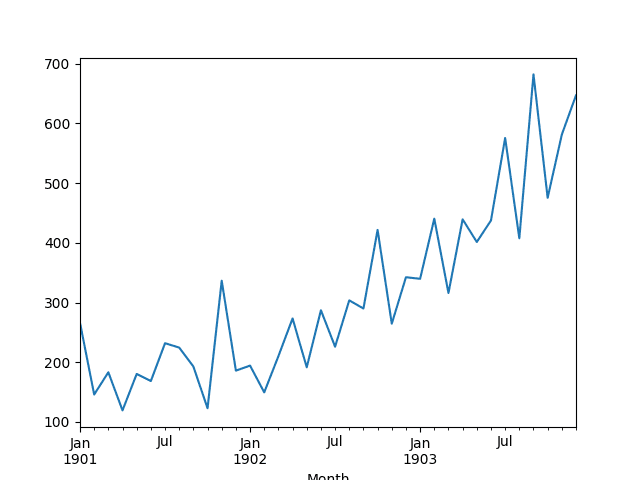
Running the example loads the dataset as a Pandas Series and prints the first 5 rows.
1
2
3
4
5
6
7
Month
1901-01-01 266.0
1901-02-01 145.9
1901-03-01 183.1
1901-04-01 119.3
1901-05-01 180.3
Name: Sales, dtype: float64
A line plot of the series is then created showing a clear increasing trend.
Line Plot of Shampoo Sales Dataset
Next, we will take a look at the LSTM configuration and test harness used in the experiment.
Experimental Test Harness
This section describes the test harness used in this tutorial.
Data Split
We will split the Shampoo Sales dataset into two parts: a training and a test set.
The first two years of data will be taken for the training dataset and the remaining one year of data will be used for the test set.
Models will be developed using the training dataset and will make predictions on the test dataset.
The persistence forecast (naive forecast) on the test dataset achieves an error of 136.761 monthly shampoo sales. This provides a lower acceptable bound of performance on the test set.
Model Evaluation
A rolling-forecast scenario will be used, also called walk-forward model validation.
Each time step of the test dataset will be walked one at a time. A model will be used to make a forecast for the time step, then the actual expected value from the test set will be taken and made available to the model for the forecast on the next time step.
This mimics a real-world scenario where new Shampoo Sales observations would be available each month and used in the forecasting of the following month.
This will be simulated by the structure of the train and test datasets.
All forecasts on the test dataset will be collected and an error score calculated to summarize the skill of the model. The root mean squared error (RMSE) will be used as it punishes large errors and results in a score that is in the same units as the forecast data, namely monthly shampoo sales.
Data Preparation
Before we can fit an LSTM model to the dataset, we must transform the data.
The following three data transforms are performed on the dataset prior to fitting a model and making a forecast.
Transform the time series data so that it is stationary. Specifically, a lag=1 differencing to remove the increasing trend in the data.
Transform the time series into a supervised learning problem. Specifically, the organization of data into input and output patterns where the observation at the previous time step is used as an input to forecast the observation at the current time step
Transform the observations to have a specific scale. Specifically, to rescale the data to values between -1 and 1 to meet the default hyperbolic tangent activation function of the LSTM model.
These transforms are inverted on forecasts to return them into their original scale before calculating and error score.
LSTM Model
We will use a base stateful LSTM model with 1 neuron fit for 500 epochs.
A batch size of 1 is required as we will be using walk-forward validation and making one-step forecasts for each of the final 12 months of test data.
A batch size of 1 means that the model will be fit using online training (as opposed to batch training or mini-batch training). As a result, it is expected that the model fit will have some variance.
Ideally, more training epochs would be used (such as 1000 or 1500), but this was truncated to 500 to keep run times reasonable.
The model will be fit using the efficient ADAM optimization algorithm and the mean squared error loss function.
Experimental Runs
Each experimental scenario will be run 10 times.
The reason for this is that the random initial conditions for an LSTM network can result in very different results each time a given configuration is trained.
Let’s dive into the experiments.
Experiments with Features
We will perform 5 experiments; each will use a different number of lag observations as features from 1 to 5.
A representation with a 1 input feature would be the default representation when using a stateful LSTM. Using 2 to 5 features is contrived. The hope would be that the additional context from the lagged observations may improve performance of the predictive model.
The univariate time series is converted to a supervised learning problem before training the model. The specified number of features defines the number of input variables (X) used to predict the next observation (y). As such, for each feature used in the representation, that many rows must be removed from the beginning of the dataset. This is because there are no prior observations to use as features for the first values in the dataset.
The complete code listing for testing 1 input feature is provided below.
The features parameter in the run() function is varied from 1 to 5 for each of the 5 experiments. In addition, the results are saved to file at the end of the experiment and this filename must also be changed for each different experimental run, e.g. experiment_features_1.csv, experiment_features_2.csv, etc.
1
2
3
4
5
6
7
8
9
10
11
12
13
14
15
16
17
18
19
20
21
22
23
24
25
26
27
28
29
30
31
32
33
34
35
36
37
38
39
40
41
42
43
44
45
46
47
48
49
50
51
52
53
54
55
56
57
58
59
60
61
62
63
64
65
66
67
68
69
70
71
72
73
74
75
76
77
78
79
80
81
82
83
84
85
86
87
88
89
90
91
92
93
94
95
96
97
98
99
100
101
102
103
104
105
106
107
108
109
110
111
112
113
114
115
116
117
118
119
120
121
122
123
124
125
126
127
128
129
130
131
from pandas import DataFrame
from pandas import Series
from pandas import concat
from pandas import read_csv
from pandas import datetime
from sklearn.metrics import mean_squared_error
from sklearn.preprocessing import MinMaxScaler
from keras.models import Sequential
from keras.layers import Dense
from keras.layers import LSTM
from math import sqrt
import matplotlib
import numpy
from numpy import concatenate
# date-time parsing function for loading the dataset
def parser(x):
returndatetime.strptime('190'+x,'%Y-%m')
# frame a sequence as a supervised learning problem
Run the 5 different experiments for the 5 different numbers of features.
You can run them in parallel if you have sufficient memory and CPU resources. GPU resources are not required for these experiments and runs should be complete in minutes to tens of minutes.
After running the experiments, you should have 5 files containing the results, as follows:
experiment_features_1.csv
experiment_features_2.csv
experiment_features_3.csv
experiment_features_4.csv
experiment_features_5.csv
We can write some code to load and summarize these results.
Specifically, it is useful to review both descriptive statistics from each run and compare the results for each run using a box and whisker plot.
Running the code first prints descriptive statistics for each set of results.
Note: Your results may vary given the stochastic nature of the algorithm or evaluation procedure, or differences in numerical precision. Consider running the example a few times and compare the average outcome.
We can see from the average performance alone that the default of using a single feature resulted in the best performance. This is also shown when reviewing the median test RMSE (50th percentile).
max 122.341580 149.807155 152.412861 123.006088 164.598542
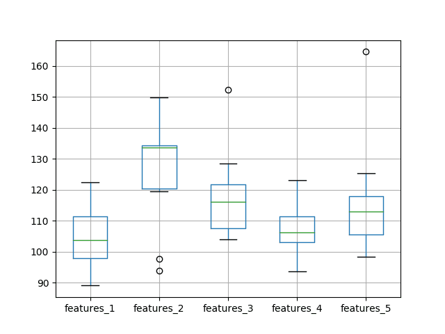
A box and whisker plot comparing the distributions of results is also created.
The plot tells the same story as the descriptive statistics. The test RMSE seems to leap up with 2 features and trend upward as the number of features is increased.
Box and Whisker Plot of Test RMSE vs The Number of Input Features
The expectation of decreased error with the increase of features was not observed, at least with the dataset and LSTM configuration used.
This raises the question as to whether the capacity of the network is a limiting factor. We will look at this in the next section.
Experiments with Features and Neurons
The number of neurons (also called units) in the LSTM network defines its learning capacity.
It is possible that in the previous experiments the use of one neuron limited the learning capacity of the network such that it was not capable of making effective use of the lagged observations as features.
We can repeat the above experiments and increase the number of neurons in the LSTM with the increase in features and see if it results in an increase in performance.
This can be achieved by changing the line in the experiment function from:
In addition, we can keep the results written to file separate from the results from the first experiment by adding a “_neurons” suffix to the filenames, for example, changing:
After running these experiments, you should have 5 result files.
experiment_features_1_neurons.csv
experiment_features_2_neurons.csv
experiment_features_3_neurons.csv
experiment_features_4_neurons.csv
experiment_features_5_neurons.csv
As in the previous experiment, we can load the results, calculate descriptive statistics, and create a box and whisker plot. The complete code listing is below.
Running the code first prints descriptive statistics from each of the 5 experiments.
Note: Your results may vary given the stochastic nature of the algorithm or evaluation procedure, or differences in numerical precision. Consider running the example a few times and compare the average outcome.
The results tell a different story to the first set of experiments with a one neuron LSTM. The average test RMSE appears lowest when the number of neurons and the number of features is set to one, then error increases as neurons and features are increased.
max 146.638148 206.760081 170.899267 188.911768 250.685187
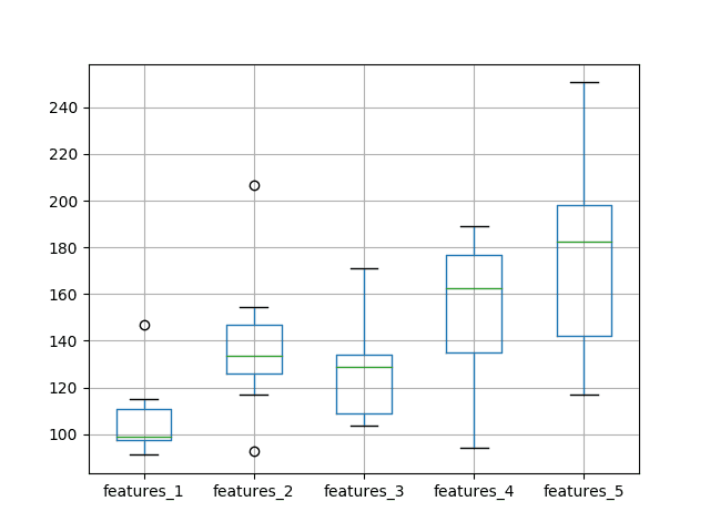
A box and whisker plot is created to compare the distributions.
The trend in spread and median performance almost shows a linear increase in test RMSE as the number of neurons and input features is increased.
The linear trend may suggest that the increase network capacity is not given sufficient time to fit the data. Perhaps an increase in the number of epochs would be required as well.
Box and Whisker Plot of Test RMSE vs The Number of Neurons and Input Features
Experiments with Features and Neurons More Epochs
In this section, we repeat the above experiment to increase the number of neurons with the number of features but double the number of training epochs from 500 to 1000.
This can be achieved by changing the line in the experiment function from:
In addition, we can keep the results written to file separate from the results from the previous experiment by adding a “1000” suffix to the filenames, for example, changing:
After running these experiments, you should have 5 result files.
experiment_features_1_neurons1000.csv
experiment_features_2_neurons1000.csv
experiment_features_3_neurons1000.csv
experiment_features_4_neurons1000.csv
experiment_features_5_neurons1000.csv
As in the previous experiment, we can load the results, calculate descriptive statistics, and create a box and whisker plot. The complete code listing is below.
Running the code first prints descriptive statistics from each of the 5 experiments.
Note: Your results may vary given the stochastic nature of the algorithm or evaluation procedure, or differences in numerical precision. Consider running the example a few times and compare the average outcome.
The results tell a very similar story to the previous experiment with half the number of training epochs. On average, a model with 1 input feature and 1 neuron outperformed the other configurations.
max 133.270446 204.260072 242.186747 288.907803 335.595974
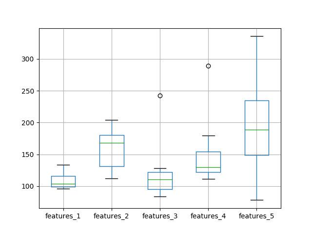
A box and whisker plot was also created to compare the distributions. In the plot, we see the same trend as was clear in the descriptive statistics.
At least on this problem and with the chosen LSTM configuration, we do not see any clear benefit in increasing the number of input features.
Box and Whisker Plot of Test RMSE vs The Number of Neurons and Input Features and 1000 Epochs
Extensions
This section lists some areas for further investigation that you may consider exploring.
Diagnostic Run Plots. It may be helpful to review plots of train and test RMSE over epochs for multiple runs for a given experiment. This might help tease out whether overfitting or underfitting is taking place, and in turn, methods to address it.
Increase Repeats. Using 10 repeats results in a relatively small population of test RMSE results. It is possible that increasing repeats to 30 or 100 (or even higher) may result in a more stable outcome.
Did you explore any of these extensions?
Share your findings in the comments below; I’d love to hear what you found.
Summary
In this tutorial, you discovered how to investigate using lagged observations as input features in an LSTM network.
Specifically, you learned:
How to develop a robust test harness for experimenting with input representation with LSTMs.
How to use lagged observations as input features for time series forecasting with LSTMs.
How to increase the learning capacity of the network with the increase of input features.
You discovered that the expectation that “the use of lagged observations as input features improves model skill” did not decrease the test RMSE on the chosen problem and LSTM configuration.
Do you have any questions?
Ask your questions in the comments below and I will do my best to answer them.
Develop Deep Learning models for Time Series Today!
When using multiple features, is a stateful model the same as a stateless one with timesteps? Can you use timesteps in a stateful model with multiple features?
Time steps are the past observations that the network will learn from (e.g. backpropagation through time). I have a few posts on BPTT coming out on the blog soon.
Features are different measurements taken at a given time step (e.g. pressure and temperature).
So we can take time steps and features just 2 type of LSTM’s input?
And for multi-dimension input , just one neuron in input layer , does it really work? And does the number of input layer’s neuron of LSTM need to be same as the input’s dimension(time steps’ dimension +features’ dimension ) like the traditional BP Neural Network?
reading the code it seems that you shape the data to give as input (X variable) such that:
X = X.reshape(X.shape[0], 1, X.shape[1])
but if you give more than one month sales as input shouldn’t you increase the number of time steps and keeping the number of features equal to 1 (only sales are analysed, not other features) ?
where am I wrong?
The promise of LSTMs (I have a scheduled post on this) is that they can learn the temporal dependence. That you just feed in sequences and do not have to specify the required window/lag (e.g. outcome from an ACF/PACF analysis).
And except that the LTSM do not have to specify the required window/lag ,is the LSTM’s prediction accuracy better than ARIMA or the LSTM can do better than other tradition method thanks to its special model struction and deep layers?
Thanks Jason, yet again a very well structured blog post. I am learning a lot from this set of posts on time series forecasting using sequence models. I have two questions for you:
1) What affect does adding more layers (going deeper) to the network have? More specifically, how do you decide when to increase number of neurons and when to make the network deeper (more layers)?
2) This might be a broad question, but specifically for time series forecasting, what “size” of data do you think is “good enough”? If I have less time series data for a problem, is it possible to transfer learn from another LSTM?
More layers mean more hierarchical representational capacity, but slower to train and perhaps more likely to overfit. Try different configurations on your problem.
As much data as you can get.
You may be able to do transfer learning, I have not read anything about it for time series with LSTMs.
I am new to deep learning and LSTM. I have a very simple question. I have taken a sample of demands for 50 time steps and I am trying to forecast the demand value for the next 10 time steps using the sample to train the model.
But unfortunately, the closest I came is splitting the sample demands into 67 training % and 33 testing % and my forecast is only forecasting for the 33%. Can anybody help me with this issue?
I have borrowed your code and put it in the in github explaining this issue.
Thank you so much for these posts; they are so helpful!
I have a question about the rolling forecast methodology. Why would you not re-fit the LSTM model after each time step? The advantage of the walk-forward validation seems to be that the model can ‘work’ in the way reality works – when making a prediction, the model has all the observations to date up until that particular time.
The reason why I would expect one would not only use the new time step’s most recent x data at the point of prediction, but also re-train the model to include the latest x,y information available up until that point would be if there were significant instability over time in the weights/parameters themselves, that would warrant a model that itself ‘rolls forward’, not just providing the most up to date x data.
There would also be computational time costs.
Am I thinking through this question correctly? That it would not really be advisable to roll forward the training set as well, re-fitting a lot of models, simply due to the fact that 1. we hope the parameters/weights are not so unstable that it would make a material difference, and 2. time costs?
Hi Jason, I don’t usually comment on these but I absolutely love your code structure! No doubt I will be using this functional approach in the future – it seems debugging would be far less painful.
I’m a newbie who’s just built his first LSTM model for stock predicting as an exercise and have found my way here trying to fix a problem. I’m using multiple features including Open price, High, Low, and Volume to predict Close price. I find that regardless of what hyperparameters I fiddle with, my prediction is always ‘lagging’ behind the real value, similar to sinusoids being out of phase with one another. Is this a problem that you have seen before with LSTM time series predictions? Perhaps something to do with the memory of the cell?
Very helpful article, thanks! I have a question regarding the number of inputs in the fit_lstm function. In the main body of the code this function takes 4 values as inputs but in the section ‘Experiments with Features and Neurons More Epochs’ there is a change to the number of inputs (from 4 to 5) in both lines of the fit_lstm function. Is that possible to provide some details regarding this change?
Thank you for the great article. I am trying to find out if there is away to find out feature importance (which features are most important?) in the LSTM model but can’t find that from Keras’ LSTM model. Is it even possible?
Hi Jason, can’t we use methods like Correlation Feature Selection and Mutual Information Feature Selection as you describe in your post on “Feature Selection for Regression Data” for LSTM?
I’m new in times series using LSTM and I have a specific problem there I’m trying to solve but I can’t find good material about.
I have many instancies of specific bearings temperatures,. (About 500 bearings ). The goal it’s to find a tendency when a bearing has a problem. So, Is it possible to train my LSTM with many instancies?
The variable temperature between each one it’s almost the same, but when the bearing has a problem, the temperature has a tendency.
Hello Jason. I have run a similar experiment:
– I have daily data for 2 years of amount spent, which I log transform
– I also use the walk-forward validation but predict several days ahead
– I run 2 scenarios:
1. A simple one: I used as input just 200 lags of the variable I am predicting (amount) ;
2. A more complicated one: I add to the input 1 numeric feature and 6 categorical ones such as holiday (1/0), weekend (1/0), year, month, day etc. I transform each original categorical feature into n-1 dummies and end up feeding the network with a total of 47 features of length 200 ( number of lags).
– My training set contains 300 samples(rows), while the validation contains 60 samples;
In the complicated scenario, the input is huge and slows down training. So, I could hardly experiment with different parameters (epochs, layers, input nodes) and come up with an optimal model. I was wondering what would you advise me on experimenting/changing right away. For example, adding more input nodes (currently set to 1000), adding more layers, decreasing the number of lags and thus increase the number of samples. I am basically troubled by the ratio of number of features to the number of samples and would adding the additional features be redundant with so few samples.
1. expanding the train size by 1, and compare it with the next one.
You mentioned that we need to fix the mnimum number of observation and you fixed as 500 for the first train size at that link. So train size would be 500, 501, 502,503,,…len(data)-1.
then, as I understood, while rolling(increasing the train size) or for each rolling, are we updating the model? or just record the error?
However, I do not see any part that you used walk forward CV here with minimum number of observation…. Or, am I missing something?
Where is the part you fix the ‘minimum number of observation’ and update the model here?
Hi Jason. I was wondering what is the difference between formulating lags as extra features (as is used in this tutorial) vs using time steps to add lags.
Basically for every sample there’s #lags time steps which contain 1 feature: the lagged y value (at x, x-1, x-2 etc.).
I’m pretty sure I’ve seen examples using the second method but I can’t really find any explanation/comparison about this anywhere.
I hope you can answer this!
Hi Jason, with lags as extra features, would it be correct to also use lag time steps, say each sample being L x F, where L is the lagged time steps (t, t-1, …, t-L) in each of the F input features? All but one features are lagged versions of the uni-variate input series.
Given in a dataset, the dataset has high temporal variation and seasonality.
Say, every 3,6,7,8,9 month have very high values for like a week,
the other months have low values(peaks)
I was able to capture the low peak values but not able to capture high peaks values.
To be specific, I am trying to build a model for riverflows. The riverflows are high when rainfall is high.. the other times they stay low.. I am not sure how to capture the high peak signals.
I am working with grid workload archive dataset ,while i am predicting the incoming job waiting time ,how can i consider input variable to predict the output variable .. I does have requested time , average cpu used and few attributes , can lstm train the input variable to give output variable
Thank you for another detailed blog, your blogs has been tremendously helpful.
I have a question regarding the theoretical usefulness of increasing the input times steps for univariate data prediction using LSTM, does all past time steps not automatically get carried forward through the structure of LSTM?
Background:
I’m comparing several methods for hourly water demand prediction, differing to the shampoo data, the hourly demand data is much longer and there is a great sense of periodicity within the data itself.
Neural network and random forecast have all performed well when the input time step is equal or greater than the data period (24 hours), I initially assumed the same for LSTM, but from my limited understanding, past features are automatically carried forward through all blocks, thus limiting the need for repeating features; however, my work has found that increasing the input time step count to 24 massively increases prediction accuracy, similar to neural network and random forecast.
I have started LSTM from another one of your blog from 2016 (Time Series Prediction with LSTM Recurrent Neural Networks in Python with Keras), I’ve modified its structure to support multiple input as well as output, I’m currently reaffirming my previous results with the code from this blog.
Thank you for your blog, I get confused and I do not understand about your second plot and how to recognize by increasing the feature the error does not decrease (in test RMSE)
where you mentioned ” Generally we would not select lag obs as the time steps for the LSTM, instead we would provide all of the time steps and lear the LSTM learn what to use to make good predictions.” and next “It can be useful for linear models, and when developing static ML models (not LSTM).”
So before i try to fully understand this blog, i would really appreciate your comment to help me understand this 2 blog “How to use lagged observations as input features for time series forecasting with LSTMs”. Thank you
hi jason great work. just curious to know one thing. in one article you have used output of supervised learning as time steps and in this article you have used that output as features so where exactly the difference lies? it makes me feel as if time steps and features are interchangeable.


When using multiple features, is a stateful model the same as a stateless one with timesteps? Can you use timesteps in a stateful model with multiple features?
It really depends on how you structure your data.
Stateless with all data in a batch or all time steps in a sample within a batch is the same as stateful.
I hope that makes things clearer. Also see this post:
https://machinelearningmastery.com/stateful-stateless-lstm-time-series-forecasting-python/
Hi,Dr.Jason Brownlee.I am confused that difference between time_steps and features in a LSTM input of Keras. Can you explain with an example?
Great question.
Time steps are the past observations that the network will learn from (e.g. backpropagation through time). I have a few posts on BPTT coming out on the blog soon.
Features are different measurements taken at a given time step (e.g. pressure and temperature).
Does that help?
Thanks for Dr.Jason Brownlee’s reply.
So we can take time steps and features just 2 type of LSTM’s input?
And for multi-dimension input , just one neuron in input layer , does it really work? And does the number of input layer’s neuron of LSTM need to be same as the input’s dimension(time steps’ dimension +features’ dimension ) like the traditional BP Neural Network?
No, the number of memory cells in the input layer does not have to match the number of input features or time steps.
reading the code it seems that you shape the data to give as input (X variable) such that:
X = X.reshape(X.shape[0], 1, X.shape[1])
but if you give more than one month sales as input shouldn’t you increase the number of time steps and keeping the number of features equal to 1 (only sales are analysed, not other features) ?
where am I wrong?
Good question, this will help regarding the shape of input data for LSTMs:
https://machinelearningmastery.com/faq/single-faq/what-is-the-difference-between-samples-timesteps-and-features-for-lstm-input
Compared to traditional method ,like AR, MA and ARIMA , What does the LSTM’s advantages in Time Series Forecasting?
Great question.
The promise of LSTMs (I have a scheduled post on this) is that they can learn the temporal dependence. That you just feed in sequences and do not have to specify the required window/lag (e.g. outcome from an ACF/PACF analysis).
And except that the LTSM do not have to specify the required window/lag ,is the LSTM’s prediction accuracy better than ARIMA or the LSTM can do better than other tradition method thanks to its special model struction and deep layers?
It may be, that is problem specific (e.g. no free lunch).
Thanks Jason, yet again a very well structured blog post. I am learning a lot from this set of posts on time series forecasting using sequence models. I have two questions for you:
1) What affect does adding more layers (going deeper) to the network have? More specifically, how do you decide when to increase number of neurons and when to make the network deeper (more layers)?
2) This might be a broad question, but specifically for time series forecasting, what “size” of data do you think is “good enough”? If I have less time series data for a problem, is it possible to transfer learn from another LSTM?
Looking forward to your response!
More layers mean more hierarchical representational capacity, but slower to train and perhaps more likely to overfit. Try different configurations on your problem.
As much data as you can get.
You may be able to do transfer learning, I have not read anything about it for time series with LSTMs.
Hi Jason,
Thank you for your wonderful post.
I am new to deep learning and LSTM. I have a very simple question. I have taken a sample of demands for 50 time steps and I am trying to forecast the demand value for the next 10 time steps using the sample to train the model.
But unfortunately, the closest I came is splitting the sample demands into 67 training % and 33 testing % and my forecast is only forecasting for the 33%. Can anybody help me with this issue?
I have borrowed your code and put it in the in github explaining this issue.
Thank you in advance.
https://github.com/ukeshchawal/hello-world/blob/master/trial.ipynb
See this post for ways of evaluating time series forecasting methods:
https://machinelearningmastery.com/backtest-machine-learning-models-time-series-forecasting/
Hi Jason,
Thank you so much for these posts; they are so helpful!
I have a question about the rolling forecast methodology. Why would you not re-fit the LSTM model after each time step? The advantage of the walk-forward validation seems to be that the model can ‘work’ in the way reality works – when making a prediction, the model has all the observations to date up until that particular time.
The reason why I would expect one would not only use the new time step’s most recent x data at the point of prediction, but also re-train the model to include the latest x,y information available up until that point would be if there were significant instability over time in the weights/parameters themselves, that would warrant a model that itself ‘rolls forward’, not just providing the most up to date x data.
There would also be computational time costs.
Am I thinking through this question correctly? That it would not really be advisable to roll forward the training set as well, re-fitting a lot of models, simply due to the fact that 1. we hope the parameters/weights are not so unstable that it would make a material difference, and 2. time costs?
Thank you!
You can and I would recommend testing it to see if it lists skill.
Here is an example:
https://machinelearningmastery.com/update-lstm-networks-training-time-series-forecasting/
Hi Jason, I don’t usually comment on these but I absolutely love your code structure! No doubt I will be using this functional approach in the future – it seems debugging would be far less painful.
I’m a newbie who’s just built his first LSTM model for stock predicting as an exercise and have found my way here trying to fix a problem. I’m using multiple features including Open price, High, Low, and Volume to predict Close price. I find that regardless of what hyperparameters I fiddle with, my prediction is always ‘lagging’ behind the real value, similar to sinusoids being out of phase with one another. Is this a problem that you have seen before with LSTM time series predictions? Perhaps something to do with the memory of the cell?
Thanks Ayush!
Yes, LSTMs are not great at this type of problem. I’d recommend an MLP instead.
Hi Jason, I am wondering why you recommend MLP for his model instead of LSTM?
Generally LSTMs perform poorly for time series. I find MLPs and CNNs often perform better.
Hi Jason,
Very helpful article, thanks! I have a question regarding the number of inputs in the fit_lstm function. In the main body of the code this function takes 4 values as inputs but in the section ‘Experiments with Features and Neurons More Epochs’ there is a change to the number of inputs (from 4 to 5) in both lines of the fit_lstm function. Is that possible to provide some details regarding this change?
I don’t recall. Can you point to the specific code change you’re referring to?
Hi Jason,
Thank you for the great article. I am trying to find out if there is away to find out feature importance (which features are most important?) in the LSTM model but can’t find that from Keras’ LSTM model. Is it even possible?
I have not seen feature importance measures for LSTMs sorry. Perhaps try searching on scholar.google.com?
Hi Jason, can’t we use methods like Correlation Feature Selection and Mutual Information Feature Selection as you describe in your post on “Feature Selection for Regression Data” for LSTM?
Perhaps try them and see.
Hello, Jason.
I’m new in times series using LSTM and I have a specific problem there I’m trying to solve but I can’t find good material about.
I have many instancies of specific bearings temperatures,. (About 500 bearings ). The goal it’s to find a tendency when a bearing has a problem. So, Is it possible to train my LSTM with many instancies?
The variable temperature between each one it’s almost the same, but when the bearing has a problem, the temperature has a tendency.
Do you know any good article?
Sounds like a good project.
Generally I would recommend this process to work through your problem:
https://machinelearningmastery.com/start-here/#process
Perhaps this material on time series forecasting will be helpful background:
https://machinelearningmastery.com/start-here/#timeseries
Hello Jason. I have run a similar experiment:
– I have daily data for 2 years of amount spent, which I log transform
– I also use the walk-forward validation but predict several days ahead
– I run 2 scenarios:
1. A simple one: I used as input just 200 lags of the variable I am predicting (amount) ;
2. A more complicated one: I add to the input 1 numeric feature and 6 categorical ones such as holiday (1/0), weekend (1/0), year, month, day etc. I transform each original categorical feature into n-1 dummies and end up feeding the network with a total of 47 features of length 200 ( number of lags).
– My training set contains 300 samples(rows), while the validation contains 60 samples;
In the complicated scenario, the input is huge and slows down training. So, I could hardly experiment with different parameters (epochs, layers, input nodes) and come up with an optimal model. I was wondering what would you advise me on experimenting/changing right away. For example, adding more input nodes (currently set to 1000), adding more layers, decreasing the number of lags and thus increase the number of samples. I am basically troubled by the ratio of number of features to the number of samples and would adding the additional features be redundant with so few samples.
It’s a tough question.
I try to tune models with small samples then scale up. Try that.
The framing always seems to offer the most leverage when I start thinking hard about a given prediction problem.
I also have a ton of advice here that might give you ideas:
https://machinelearningmastery.com/improve-deep-learning-performance/
Hi! I hope this finds you well! I really aprpeciate your post!
I have seen your post about walk forwarding cv: https://machinelearningmastery.com/backtest-machine-learning-models-time-series-forecasting/
and I think I understood.
1. expanding the train size by 1, and compare it with the next one.
You mentioned that we need to fix the mnimum number of observation and you fixed as 500 for the first train size at that link. So train size would be 500, 501, 502,503,,…len(data)-1.
then, as I understood, while rolling(increasing the train size) or for each rolling, are we updating the model? or just record the error?
However, I do not see any part that you used walk forward CV here with minimum number of observation…. Or, am I missing something?
Where is the part you fix the ‘minimum number of observation’ and update the model here?
Thank you so much !
In many of the neural net cases, I do not update the model each walk forward, it’s too computationally expensive.
Hi Jason. I was wondering what is the difference between formulating lags as extra features (as is used in this tutorial) vs using time steps to add lags.
Basically for every sample there’s #lags time steps which contain 1 feature: the lagged y value (at x, x-1, x-2 etc.).
I’m pretty sure I’ve seen examples using the second method but I can’t really find any explanation/comparison about this anywhere.
I hope you can answer this!
The key is BPTT operates over time steps.
It’s the difference between learning from the sequence and learning a static input/output mapping.
This post might help:
https://machinelearningmastery.com/gentle-introduction-backpropagation-time/
Hi Jason, with lags as extra features, would it be correct to also use lag time steps, say each sample being L x F, where L is the lagged time steps (t, t-1, …, t-L) in each of the F input features? All but one features are lagged versions of the uni-variate input series.
Hi Jason,
Given in a dataset, the dataset has high temporal variation and seasonality.
Say, every 3,6,7,8,9 month have very high values for like a week,
the other months have low values(peaks)
I was able to capture the low peak values but not able to capture high peaks values.
To be specific, I am trying to build a model for riverflows. The riverflows are high when rainfall is high.. the other times they stay low.. I am not sure how to capture the high peak signals.
Perhaps you can classify observations as high/low river flow, then develop separate models for those cases?
Thanks for sharing this. I wonder if you have any tutorial on the unsupervised approach – auto-econder on a data with a similar format ?
You’re welcome.
Yes, see this:
https://machinelearningmastery.com/lstm-autoencoders/
I am working with grid workload archive dataset ,while i am predicting the incoming job waiting time ,how can i consider input variable to predict the output variable .. I does have requested time , average cpu used and few attributes , can lstm train the input variable to give output variable
Yes, perhaps start here:
https://machinelearningmastery.com/start-here/#deep_learning_time_series
Hi Dr Brownlwee,
Thank you for another detailed blog, your blogs has been tremendously helpful.
I have a question regarding the theoretical usefulness of increasing the input times steps for univariate data prediction using LSTM, does all past time steps not automatically get carried forward through the structure of LSTM?
Background:
I’m comparing several methods for hourly water demand prediction, differing to the shampoo data, the hourly demand data is much longer and there is a great sense of periodicity within the data itself.
Neural network and random forecast have all performed well when the input time step is equal or greater than the data period (24 hours), I initially assumed the same for LSTM, but from my limited understanding, past features are automatically carried forward through all blocks, thus limiting the need for repeating features; however, my work has found that increasing the input time step count to 24 massively increases prediction accuracy, similar to neural network and random forecast.
I have started LSTM from another one of your blog from 2016 (Time Series Prediction with LSTM Recurrent Neural Networks in Python with Keras), I’ve modified its structure to support multiple input as well as output, I’m currently reaffirming my previous results with the code from this blog.
You’re welcome.
Theory is not going to help – I recommend designing controlled experiments in order to discover what works best for your specific dataset and model.
Hi Dr. Brownlwee
Thank you for your blog, I get confused and I do not understand about your second plot and how to recognize by increasing the feature the error does not decrease (in test RMSE)
We can see that RMSE is not decreased because the distributions and medians skew higher with the increase in the number of features.
Hi Jason, i am new to LSTM and i was reading your other blog
Feature Selection for Time Series Forecasting with Python
https://machinelearningmastery.com/feature-selection-time-series-forecasting-python/
where you mentioned ” Generally we would not select lag obs as the time steps for the LSTM, instead we would provide all of the time steps and lear the LSTM learn what to use to make good predictions.” and next “It can be useful for linear models, and when developing static ML models (not LSTM).”
So before i try to fully understand this blog, i would really appreciate your comment to help me understand this 2 blog “How to use lagged observations as input features for time series forecasting with LSTMs”. Thank you
Great question, this will help:
https://machinelearningmastery.com/time-series-forecasting-supervised-learning/
hi jason great work. just curious to know one thing. in one article you have used output of supervised learning as time steps and in this article you have used that output as features so where exactly the difference lies? it makes me feel as if time steps and features are interchangeable.