Given the rise of smart electricity meters and the wide adoption of electricity generation technology like solar panels, there is a wealth of electricity usage data available.
This data represents a multivariate time series of power-related variables that in turn could be used to model and even forecast future electricity consumption.
Unlike other machine learning algorithms, long short-term memory recurrent neural networks are capable of automatically learning features from sequence data, support multiple-variate data, and can output a variable length sequences that can be used for multi-step forecasting.
In this tutorial, you will discover how to develop long short-term memory recurrent neural networks for multi-step time series forecasting of household power consumption.
After completing this tutorial, you will know:
How to develop and evaluate Univariate and multivariate Encoder-Decoder LSTMs for multi-step time series forecasting.
How to develop and evaluate an CNN-LSTM Encoder-Decoder model for multi-step time series forecasting.
How to develop and evaluate a ConvLSTM Encoder-Decoder model for multi-step time series forecasting.
Kick-start your project with my new book Deep Learning for Time Series Forecasting, including step-by-step tutorials and the Python source code files for all examples.
Let’s get started.
Note: This is a reasonably advanced tutorial, if you are new to time series forecasting in Python, start here. If you are new to using deep learning for time series, start here. If you really want to get started with LSTMs for time series, start here.
Update Jun/2019: Fixed bug in to_supervised() that dropped the last week of data (thanks Markus).
Update Nov/2021: Fixed a typo (thanks Sandy)
How to Develop LSTM Models for Multi-Step Time Series Forecasting of Household Power Consumption Photo by Ian Muttoo, some rights reserved.
Tutorial Overview
This tutorial is divided into nine parts; they are:
Problem Description
Load and Prepare Dataset
Model Evaluation
LSTMs for Multi-Step Forecasting
LSTM Model With Univariate Input and Vector Output
Encoder-Decoder LSTM Model With Univariate Input
Encoder-Decoder LSTM Model With Multivariate Input
CNN-LSTM Encoder-Decoder Model With Univariate Input
ConvLSTM Encoder-Decoder Model With Univariate Input
Python Environment
This tutorial assumes you have a Python SciPy environment installed, ideally with Python 3.
You must have Keras (2.2 or higher) installed with either the TensorFlow or Theano backend.
The tutorial also assumes you have scikit-learn, Pandas, NumPy, and Matplotlib installed.
If you need help with your environment, see this tutorial:
The ‘Household Power Consumption‘ dataset is a multivariate time series dataset that describes the electricity consumption for a single household over four years.
Download the dataset and unzip it into your current working directory. You will now have the file “household_power_consumption.txt” that is about 127 megabytes in size and contains all of the observations.
We can use the read_csv() function to load the data and combine the first two columns into a single date-time column that we can use as an index.
Next, we can mark all missing values indicated with a ‘?‘ character with a NaN value, which is a float.
This will allow us to work with the data as one array of floating point values rather than mixed types (less efficient.)
1
2
3
4
# mark all missing values
dataset.replace('?',nan,inplace=True)
# make dataset numeric
dataset=dataset.astype('float32')
We also need to fill in the missing values now that they have been marked.
A very simple approach would be to copy the observation from the same time the day before. We can implement this in a function named fill_missing() that will take the NumPy array of the data and copy values from exactly 24 hours ago.
1
2
3
4
5
6
7
# fill missing values with a value at the same time one day ago
def fill_missing(values):
one_day=60*24
forrow inrange(values.shape[0]):
forcol inrange(values.shape[1]):
ifisnan(values[row,col]):
values[row,col]=values[row-one_day,col]
We can apply this function directly to the data within the DataFrame.
1
2
# fill missing
fill_missing(dataset.values)
Now we can create a new column that contains the remainder of the sub-metering, using the calculation from the previous section.
1
2
3
# add a column for for the remainder of sub metering
We can now save the cleaned-up version of the dataset to a new file; in this case we will just change the file extension to .csv and save the dataset as ‘household_power_consumption.csv‘.
1
2
# save updated dataset
dataset.to_csv('household_power_consumption.csv')
Tying all of this together, the complete example of loading, cleaning-up, and saving the dataset is listed below.
1
2
3
4
5
6
7
8
9
10
11
12
13
14
15
16
17
18
19
20
21
22
23
24
25
26
27
# load and clean-up data
from numpy import nan
from numpy import isnan
from pandas import read_csv
from pandas import to_numeric
# fill missing values with a value at the same time one day ago
Running the example creates the new file ‘household_power_consumption.csv‘ that we can use as the starting point for our modeling project.
Need help with Deep Learning for Time Series?
Take my free 7-day email crash course now (with sample code).
Click to sign-up and also get a free PDF Ebook version of the course.
Model Evaluation
In this section, we will consider how we can develop and evaluate predictive models for the household power dataset.
This section is divided into four parts; they are:
Problem Framing
Evaluation Metric
Train and Test Sets
Walk-Forward Validation
Problem Framing
There are many ways to harness and explore the household power consumption dataset.
In this tutorial, we will use the data to explore a very specific question; that is:
Given recent power consumption, what is the expected power consumption for the week ahead?
This requires that a predictive model forecast the total active power for each day over the next seven days.
Technically, this framing of the problem is referred to as a multi-step time series forecasting problem, given the multiple forecast steps. A model that makes use of multiple input variables may be referred to as a multivariate multi-step time series forecasting model.
A model of this type could be helpful within the household in planning expenditures. It could also be helpful on the supply side for planning electricity demand for a specific household.
This framing of the dataset also suggests that it would be useful to downsample the per-minute observations of power consumption to daily totals. This is not required, but makes sense, given that we are interested in total power per day.
We can achieve this easily using the resample() function on the pandas DataFrame. Calling this function with the argument ‘D‘ allows the loaded data indexed by date-time to be grouped by day (see all offset aliases). We can then calculate the sum of all observations for each day and create a new dataset of daily power consumption data for each of the eight variables.
Running the example creates a new daily total power consumption dataset and saves the result into a separate file named ‘household_power_consumption_days.csv‘.
We can use this as the dataset for fitting and evaluating predictive models for the chosen framing of the problem.
Evaluation Metric
A forecast will be comprised of seven values, one for each day of the week ahead.
It is common with multi-step forecasting problems to evaluate each forecasted time step separately. This is helpful for a few reasons:
To comment on the skill at a specific lead time (e.g. +1 day vs +3 days).
To contrast models based on their skills at different lead times (e.g. models good at +1 day vs models good at days +5).
The units of the total power are kilowatts and it would be useful to have an error metric that was also in the same units. Both Root Mean Squared Error (RMSE) and Mean Absolute Error (MAE) fit this bill, although RMSE is more commonly used and will be adopted in this tutorial. Unlike MAE, RMSE is more punishing of forecast errors.
The performance metric for this problem will be the RMSE for each lead time from day 1 to day 7.
As a short-cut, it may be useful to summarize the performance of a model using a single score in order to aide in model selection.
One possible score that could be used would be the RMSE across all forecast days.
The function evaluate_forecasts() below will implement this behavior and return the performance of a model based on multiple seven-day forecasts.
1
2
3
4
5
6
7
8
9
10
11
12
13
14
15
16
17
18
# evaluate one or more weekly forecasts against expected values
Running the function will first return the overall RMSE regardless of day, then an array of RMSE scores for each day.
Train and Test Sets
We will use the first three years of data for training predictive models and the final year for evaluating models.
The data in a given dataset will be divided into standard weeks. These are weeks that begin on a Sunday and end on a Saturday.
This is a realistic and useful way for using the chosen framing of the model, where the power consumption for the week ahead can be predicted. It is also helpful with modeling, where models can be used to predict a specific day (e.g. Wednesday) or the entire sequence.
We will split the data into standard weeks, working backwards from the test dataset.
The final year of the data is in 2010 and the first Sunday for 2010 was January 3rd. The data ends in mid November 2010 and the closest final Saturday in the data is November 20th. This gives 46 weeks of test data.
The first and last rows of daily data for the test dataset are provided below for confirmation.
The function split_dataset() below splits the daily data into train and test sets and organizes each into standard weeks.
Specific row offsets are used to split the data using knowledge of the dataset. The split datasets are then organized into weekly data using the NumPy split() function.
1
2
3
4
5
6
7
8
# split a univariate dataset into train/test sets
def split_dataset(data):
# split into standard weeks
train,test=data[1:-328],data[-328:-6]
# restructure into windows of weekly data
train=array(split(train,len(train)/7))
test=array(split(test,len(test)/7))
returntrain,test
We can test this function out by loading the daily dataset and printing the first and last rows of data from both the train and test sets to confirm they match the expectations above.
Running the example shows that indeed the train dataset has 159 weeks of data, whereas the test dataset has 46 weeks.
We can see that the total active power for the train and test dataset for the first and last rows match the data for the specific dates that we defined as the bounds on the standard weeks for each set.
This is where a model is required to make a one week prediction, then the actual data for that week is made available to the model so that it can be used as the basis for making a prediction on the subsequent week. This is both realistic for how the model may be used in practice and beneficial to the models allowing them to make use of the best available data.
We can demonstrate this below with separation of input data and output/predicted data.
1
2
3
4
5
Input, Predict
[Week1] Week2
[Week1 + Week2] Week3
[Week1 + Week2 + Week3] Week4
...
The walk-forward validation approach to evaluating predictive models on this dataset is provided below named evaluate_model().
The train and test datasets in standard-week format are provided to the function as arguments. An additional argument n_input is provided that is used to define the number of prior observations that the model will use as input in order to make a prediction.
Two new functions are called: one to build a model from the training data called build_model() and another that uses the model to make forecasts for each new standard week called forecast(). These will be covered in subsequent sections.
We are working with neural networks, and as such, they are generally slow to train but fast to evaluate. This means that the preferred usage of the models is to build them once on historical data and to use them to forecast each step of the walk-forward validation. The models are static (i.e. not updated) during their evaluation.
This is different to other models that are faster to train where a model may be re-fit or updated each step of the walk-forward validation as new data is made available. With sufficient resources, it is possible to use neural networks this way, but we will not in this tutorial.
The complete evaluate_model() function is listed below.
1
2
3
4
5
6
7
8
9
10
11
12
13
14
15
16
17
18
19
# evaluate a single model
def evaluate_model(train,test,n_input):
# fit model
model=build_model(train,n_input)
# history is a list of weekly data
history=[xforxintrain]
# walk-forward validation over each week
predictions=list()
foriinrange(len(test)):
# predict the week
yhat_sequence=forecast(model,history,n_input)
# store the predictions
predictions.append(yhat_sequence)
# get real observation and add to history for predicting the next week
Once we have the evaluation for a model, we can summarize the performance.
The function below named summarize_scores() will display the performance of a model as a single line for easy comparison with other models.
1
2
3
4
# summarize scores
def summarize_scores(name,score,scores):
s_scores=', '.join(['%.1f'%sforsinscores])
print('%s: [%.3f] %s'%(name,score,s_scores))
We now have all of the elements to begin evaluating predictive models on the dataset.
LSTMs for Multi-Step Forecasting
Recurrent neural networks, or RNNs, are specifically designed to work, learn, and predict sequence data.
A recurrent neural network is a neural network where the output of the network from one time step is provided as an input in the subsequent time step. This allows the model to make a decision as to what to predict based on both the input for the current time step and direct knowledge of what was output in the prior time step.
Perhaps the most successful and widely used RNN is the long short-term memory network, or LSTM for short. It is successful because it overcomes the challenges involved in training a recurrent neural network, resulting in stable models. In addition to harnessing the recurrent connection of the outputs from the prior time step, LSTMs also have an internal memory that operates like a local variable, allowing them to accumulate state over the input sequence.
For more information about Recurrent Neural Networks, see the post:
LSTMs offer a number of benefits when it comes to multi-step time series forecasting; they are:
Native Support for Sequences. LSTMs are a type of recurrent network, and as such are designed to take sequence data as input, unlike other models where lag observations must be presented as input features.
Multivariate Inputs. LSTMs directly support multiple parallel input sequences for multivariate inputs, unlike other models where multivariate inputs are presented in a flat structure.
Vector Output. Like other neural networks, LSTMs are able to map input data directly to an output vector that may represent multiple output time steps.
Further, specialized architectures have been developed that are specifically designed to make multi-step sequence predictions, generally referred to as sequence-to-sequence prediction, or seq2seq for short. This is useful as multi-step time series forecasting is a type of seq2seq prediction.
An example of a recurrent neural network architecture designed for seq2seq problems is the encoder-decoder LSTM.
An encoder-decoder LSTM is a model comprised of two sub-models: one called the encoder that reads the input sequences and compresses it to a fixed-length internal representation, and an output model called the decoder that interprets the internal representation and uses it to predict the output sequence.
The encoder-decoder approach to sequence prediction has proven much more effective than outputting a vector directly and is the preferred approach.
Generally, LSTMs have been found to not be very effective at auto-regression type problems. These are problems where forecasting the next time step is a function of recent time steps.
One-dimensional convolutional neural networks, or CNNs, have proven effective at automatically learning features from input sequences.
A popular approach has been to combine CNNs with LSTMs, where the CNN is as an encoder to learn features from sub-sequences of input data which are provided as time steps to an LSTM. This architecture is called a CNN-LSTM.
For more information on this architecture, see the post:
A power variation on the CNN LSTM architecture is the ConvLSTM that uses the convolutional reading of input subsequences directly within an LSTM’s units. This approach has proven very effective for time series classification and can be adapted for use in multi-step time series forecasting.
In this tutorial, we will explore a suite of LSTM architectures for multi-step time series forecasting. Specifically, we will look at how to develop the following models:
LSTM model with vector output for multi-step forecasting with univariate input data.
Encoder-Decoder LSTM model for multi-step forecasting with univariate input data.
Encoder-Decoder LSTM model for multi-step forecasting with multivariate input data.
CNN-LSTM Encoder-Decoder model for multi-step forecasting with univariate input data.
ConvLSTM Encoder-Decoder model for multi-step forecasting with univariate input data.
If you are new to using LSTMs for time series forecasting, I highly recommend the post:
The models will be developed and demonstrated on the household power prediction problem. A model is considered skillful if it achieves performance better than a naive model, which is an overall RMSE of about 465 kilowatts across a seven day forecast.
We will not focus on the tuning of these models to achieve optimal performance; instead, we will stop short at skillful models as compared to a naive forecast. The chosen structures and hyperparameters are chosen with a little trial and error. The scores should be taken as just an example rather than a study of the optimal model or configuration for the problem.
Given the stochastic nature of the models, it is good practice to evaluate a given model multiple times and report the mean performance on a test dataset. In the interest of brevity and keeping the code simple, we will instead present single-runs of models in this tutorial.
We cannot know which approach will be the most effective for a given multi-step forecasting problem. It is a good idea to explore a suite of methods in order to discover what works best on your specific dataset.
LSTM Model With Univariate Input and Vector Output
We will start off by developing a simple or vanilla LSTM model that reads in a sequence of days of total daily power consumption and predicts a vector output of the next standard week of daily power consumption.
This will provide the foundation for the more elaborate models developed in subsequent sections.
The number of prior days used as input defines the one-dimensional (1D) subsequence of data that the LSTM will read and learn to extract features. Some ideas on the size and nature of this input include:
All prior days, up to years worth of data.
The prior seven days.
The prior two weeks.
The prior one month.
The prior one year.
The prior week and the week to be predicted from one year ago.
There is no right answer; instead, each approach and more can be tested and the performance of the model can be used to choose the nature of the input that results in the best model performance.
These choices define a few things:
How the training data must be prepared in order to fit the model.
How the test data must be prepared in order to evaluate the model.
How to use the model to make predictions with a final model in the future.
A good starting point would be to use the prior seven days.
An LSTM model expects data to have the shape:
1
[samples, timesteps, features]
One sample will be comprised of seven time steps with one feature for the seven days of total daily power consumed.
The training dataset has 159 weeks of data, so the shape of the training dataset would be:
1
[159, 7, 1]
This is a good start. The data in this format would use the prior standard week to predict the next standard week. A problem is that 159 instances is not a lot to train a neural network.
A way to create a lot more training data is to change the problem during training to predict the next seven days given the prior seven days, regardless of the standard week.
This only impacts the training data, and the test problem remains the same: predict the daily power consumption for the next standard week given the prior standard week.
This will require a little preparation of the training data.
The training data is provided in standard weeks with eight variables, specifically in the shape [159, 7, 8]. The first step is to flatten the data so that we have eight time series sequences.
We then need to iterate over the time steps and divide the data into overlapping windows; each iteration moves along one time step and predicts the subsequent seven days.
We can do this by keeping track of start and end indexes for the inputs and outputs as we iterate across the length of the flattened data in terms of time steps.
We can also do this in a way where the number of inputs and outputs are parameterized (e.g. n_input, n_out) so that you can experiment with different values or adapt it for your own problem.
Below is a function named to_supervised() that takes a list of weeks (history) and the number of time steps to use as inputs and outputs and returns the data in the overlapping moving window format.
# step over the entire history one time step at a time
for_inrange(len(data)):
# define the end of the input sequence
in_end=in_start+n_input
out_end=in_end+n_out
# ensure we have enough data for this instance
ifout_end<=len(data):
x_input=data[in_start:in_end,0]
x_input=x_input.reshape((len(x_input),1))
X.append(x_input)
y.append(data[in_end:out_end,0])
# move along one time step
in_start+=1
returnarray(X),array(y)
When we run this function on the entire training dataset, we transform 159 samples into 1,100; specifically, the transformed dataset has the shapes X=[1100, 7, 1] and y=[1100, 7].
Next, we can define and fit the LSTM model on the training data.
This multi-step time series forecasting problem is an autoregression. That means it is likely best modeled where that the next seven days is some function of observations at prior time steps. This and the relatively small amount of data means that a small model is required.
We will develop a model with a single hidden LSTM layer with 200 units. The number of units in the hidden layer is unrelated to the number of time steps in the input sequences. The LSTM layer is followed by a fully connected layer with 100 nodes that will interpret the features learned by the LSTM layer. Finally, an output layer will directly predict a vector with seven elements, one for each day in the output sequence.
We will use the mean squared error loss function as it is a good match for our chosen error metric of RMSE. We will use the efficient Adam implementation of stochastic gradient descent and fit the model for 70 epochs with a batch size of 16.
The small batch size and the stochastic nature of the algorithm means that the same model will learn a slightly different mapping of inputs to outputs each time it is trained. This means results may vary when the model is evaluated. You can try running the model multiple times and calculate an average of model performance.
The build_model() below prepares the training data, defines the model, and fits the model on the training data, returning the fit model ready for making predictions.
Now that we know how to fit the model, we can look at how the model can be used to make a prediction.
Generally, the model expects data to have the same three dimensional shape when making a prediction.
In this case, the expected shape of an input pattern is one sample, seven days of one feature for the daily power consumed:
1
[1, 7, 1]
Data must have this shape when making predictions for the test set and when a final model is being used to make predictions in the future. If you change the number if input days to 14, then the shape of the training data and the shape of new samples when making predictions must be changed accordingly to have 14 time steps. It is a modeling choice that you must carry forward when using the model.
We are using walk-forward validation to evaluate the model as described in the previous section.
This means that we have the observations available for the prior week in order to predict the coming week. These are collected into an array of standard weeks called history.
In order to predict the next standard week, we need to retrieve the last days of observations. As with the training data, we must first flatten the history data to remove the weekly structure so that we end up with eight parallel time series.
Next, we need to retrieve the last seven days of daily total power consumed (feature index 0).
We will parameterize this as we did for the training data so that the number of prior days used as input by the model can be modified in the future.
1
2
# retrieve last observations for input data
input_x=data[-n_input:,0]
Next, we reshape the input into the expected three-dimensional structure.
1
2
# reshape into [1, n_input, 1]
input_x=input_x.reshape((1,len(input_x),1))
We then make a prediction using the fit model and the input data and retrieve the vector of seven days of output.
1
2
3
4
# forecast the next week
yhat=model.predict(input_x,verbose=0)
# we only want the vector forecast
yhat=yhat[0]
The forecast() function below implements this and takes as arguments the model fit on the training dataset, the history of data observed so far, and the number of input time steps expected by the model.
That’s it; we now have everything we need to make multi-step time series forecasts with an LSTM model on the daily total power consumed univariate dataset.
We can tie all of this together. The complete example is listed below.
1
2
3
4
5
6
7
8
9
10
11
12
13
14
15
16
17
18
19
20
21
22
23
24
25
26
27
28
29
30
31
32
33
34
35
36
37
38
39
40
41
42
43
44
45
46
47
48
49
50
51
52
53
54
55
56
57
58
59
60
61
62
63
64
65
66
67
68
69
70
71
72
73
74
75
76
77
78
79
80
81
82
83
84
85
86
87
88
89
90
91
92
93
94
95
96
97
98
99
100
101
102
103
104
105
106
107
108
109
110
111
112
113
114
115
116
117
118
119
120
121
122
123
124
125
126
127
128
129
130
131
# univariate multi-step lstm
from math import sqrt
from numpy import split
from numpy import array
from pandas import read_csv
from sklearn.metrics import mean_squared_error
from matplotlib import pyplot
from keras.models import Sequential
from keras.layers import Dense
from keras.layers import Flatten
from keras.layers import LSTM
# split a univariate dataset into train/test sets
def split_dataset(data):
# split into standard weeks
train,test=data[1:-328],data[-328:-6]
# restructure into windows of weekly data
train=array(split(train,len(train)/7))
test=array(split(test,len(test)/7))
returntrain,test
# evaluate one or more weekly forecasts against expected values
Running the example fits and evaluates the model, printing the overall RMSE across all seven days, and the per-day RMSE for each lead time.
Note: Your results may vary given the stochastic nature of the algorithm or evaluation procedure, or differences in numerical precision. Consider running the example a few times and compare the average outcome.
We can see that in this case, the model was skillful as compared to a naive forecast, achieving an overall RMSE of about 399 kilowatts, less than 465 kilowatts achieved by a naive model.
The plot shows that perhaps Tuesdays and Fridays are easier days to forecast than the other days and that perhaps Saturday at the end of the standard week is the hardest day to forecast.
Line Plot of RMSE per Day for Univariate LSTM with Vector Output and 7-day Inputs
We can increase the number of prior days to use as input from seven to 14 by changing the n_input variable.
1
2
# evaluate model and get scores
n_input=14
Re-running the example with this change first prints a summary of performance of the model.
Note: Your results may vary given the stochastic nature of the algorithm or evaluation procedure, or differences in numerical precision. Consider running the example a few times and compare the average outcome.
In this case, we can see a further drop in the overall RMSE to about 370 kilowatts, suggesting that further tuning of the input size and perhaps the number of nodes in the model may result in better performance.
Comparing the per-day RMSE scores we see some are better and some are worse than using seven-day inputs.
This may suggest benefit in using the two different sized inputs in some way, such as an ensemble of the two approaches or perhaps a single model (e.g. a multi-headed model) that reads the training data in different ways.
Line Plot of RMSE per Day for Univariate LSTM with Vector Output and 14-day Inputs
Encoder-Decoder LSTM Model With Univariate Input
In this section, we can update the vanilla LSTM to use an encoder-decoder model.
This means that the model will not output a vector sequence directly. Instead, the model will be comprised of two sub models, the encoder to read and encode the input sequence, and the decoder that will read the encoded input sequence and make a one-step prediction for each element in the output sequence.
The difference is subtle, as in practice both approaches do in fact predict a sequence output.
The important difference is that an LSTM model is used in the decoder, allowing it to both know what was predicted for the prior day in the sequence and accumulate internal state while outputting the sequence.
Let’s take a closer look at how this model is defined.
As before, we define an LSTM hidden layer with 200 units. This is the encoder model that will read the input sequence and will output a 200 element vector (one output per unit) that captures features from the input sequence. We will use 14 days of total power consumption as input.
We will use a simple encoder-decoder architecture that is easy to implement in Keras, that has a lot of similarity to the architecture of an LSTM autoencoder.
First, the internal representation of the input sequence is repeated multiple times, once for each time step in the output sequence. This sequence of vectors will be presented to the LSTM decoder.
1
model.add(RepeatVector(7))
We then define the decoder as an LSTM hidden layer with 200 units. Importantly, the decoder will output the entire sequence, not just the output at the end of the sequence as we did with the encoder. This means that each of the 200 units will output a value for each of the seven days, representing the basis for what to predict for each day in the output sequence.
We will then use a fully connected layer to interpret each time step in the output sequence before the final output layer. Importantly, the output layer predicts a single step in the output sequence, not all seven days at a time,
This means that we will use the same layers applied to each step in the output sequence. It means that the same fully connected layer and output layer will be used to process each time step provided by the decoder. To achieve this, we will wrap the interpretation layer and the output layer in a TimeDistributed wrapper that allows the wrapped layers to be used for each time step from the decoder.
This allows the LSTM decoder to figure out the context required for each step in the output sequence and the wrapped dense layers to interpret each time step separately, yet reusing the same weights to perform the interpretation. An alternative would be to flatten all of the structure created by the LSTM decoder and to output the vector directly. You can try this as an extension to see how it compares.
The network therefore outputs a three-dimensional vector with the same structure as the input, with the dimensions [samples, timesteps, features].
There is a single feature, the daily total power consumed, and there are always seven features. A single one-week prediction will therefore have the size: [1, 7, 1].
Therefore, when training the model, we must restructure the output data (y) to have the three-dimensional structure instead of the two-dimensional structure of [samples, features] used in the previous section.
1
2
# reshape output into [samples, timesteps, features]
Running the example fits the model and summarizes the performance on the test dataset.
Note: Your results may vary given the stochastic nature of the algorithm or evaluation procedure, or differences in numerical precision. Consider running the example a few times and compare the average outcome.
We can see that in this case, the model is skillful, achieving an overall RMSE score of about 372 kilowatts.
A line plot of the per-day RMSE is also created showing a similar pattern in error as was seen in the previous section.
Line Plot of RMSE per Day for Univariate Encoder-Decoder LSTM with 14-day Inputs
Encoder-Decoder LSTM Model With Multivariate Input
In this section, we will update the Encoder-Decoder LSTM developed in the previous section to use each of the eight time series variables to predict the next standard week of daily total power consumption.
We will do this by providing each one-dimensional time series to the model as a separate sequence of input.
The LSTM will in turn create an internal representation of each input sequence that will together be interpreted by the decoder.
Using multivariate inputs is helpful for those problems where the output sequence is some function of the observations at prior time steps from multiple different features, not just (or including) the feature being forecasted. It is unclear whether this is the case in the power consumption problem, but we can explore it nonetheless.
First, we must update the preparation of the training data to include all of the eight features, not just the one total daily power consumed. It requires a single line change:
1
X.append(data[in_start:in_end,:])
The complete to_supervised() function with this change is listed below.
The same model architecture and configuration is used directly, although we will increase the number of training epochs from 20 to 50 given the 8-fold increase in the amount of input data.
The complete example is listed below.
1
2
3
4
5
6
7
8
9
10
11
12
13
14
15
16
17
18
19
20
21
22
23
24
25
26
27
28
29
30
31
32
33
34
35
36
37
38
39
40
41
42
43
44
45
46
47
48
49
50
51
52
53
54
55
56
57
58
59
60
61
62
63
64
65
66
67
68
69
70
71
72
73
74
75
76
77
78
79
80
81
82
83
84
85
86
87
88
89
90
91
92
93
94
95
96
97
98
99
100
101
102
103
104
105
106
107
108
109
110
111
112
113
114
115
116
117
118
119
120
121
122
123
124
125
126
127
128
129
130
131
132
133
134
135
# multivariate multi-step encoder-decoder lstm
from math import sqrt
from numpy import split
from numpy import array
from pandas import read_csv
from sklearn.metrics import mean_squared_error
from matplotlib import pyplot
from keras.models import Sequential
from keras.layers import Dense
from keras.layers import Flatten
from keras.layers import LSTM
from keras.layers import RepeatVector
from keras.layers import TimeDistributed
# split a univariate dataset into train/test sets
def split_dataset(data):
# split into standard weeks
train,test=data[1:-328],data[-328:-6]
# restructure into windows of weekly data
train=array(split(train,len(train)/7))
test=array(split(test,len(test)/7))
returntrain,test
# evaluate one or more weekly forecasts against expected values
Running the example fits the model and summarizes the performance on the test dataset.
Experimentation found that this model appears less stable than the univariate case and may be related to the differing scales of the input eight variables.
Note: Your results may vary given the stochastic nature of the algorithm or evaluation procedure, or differences in numerical precision. Consider running the example a few times and compare the average outcome.
We can see that in this case, the model is skillful, achieving an overall RMSE score of about 376 kilowatts.
Line Plot of RMSE per Day for Multivariate Encoder-Decoder LSTM with 14-day Inputs
CNN-LSTM Encoder-Decoder Model With Univariate Input
A convolutional neural network, or CNN, can be used as the encoder in an encoder-decoder architecture.
The CNN does not directly support sequence input; instead, a 1D CNN is capable of reading across sequence input and automatically learning the salient features. These can then be interpreted by an LSTM decoder as per normal. We refer to hybrid models that use a CNN and LSTM as CNN-LSTM models, and in this case we are using them together in an encoder-decoder architecture.
The CNN expects the input data to have the same 3D structure as the LSTM model, although multiple features are read as different channels that ultimately have the same effect.
We will simplify the example and focus on the CNN-LSTM with univariate input, but it can just as easily be updated to use multivariate input, which is left as an exercise.
As before, we will use input sequences comprised of 14 days of daily total power consumption.
We will define a simple but effective CNN architecture for the encoder that is comprised of two convolutional layers followed by a max pooling layer, the results of which are then flattened.
The first convolutional layer reads across the input sequence and projects the results onto feature maps. The second performs the same operation on the feature maps created by the first layer, attempting to amplify any salient features. We will use 64 feature maps per convolutional layer and read the input sequences with a kernel size of three time steps.
The max pooling layer simplifies the feature maps by keeping 1/4 of the values with the largest (max) signal. The distilled feature maps after the pooling layer are then flattened into one long vector that can then be used as input to the decoding process.
Running the example fits the model and summarizes the performance on the test dataset.
A little experimentation showed that using two convolutional layers made the model more stable than using just a single layer.
Note: Your results may vary given the stochastic nature of the algorithm or evaluation procedure, or differences in numerical precision. Consider running the example a few times and compare the average outcome.
We can see that in this case the model is skillful, achieving an overall RMSE score of about 372 kilowatts.
Line Plot of RMSE per Day for Univariate Encoder-Decoder CNN LSTM with 14-day Inputs
ConvLSTM Encoder-Decoder Model With Univariate Input
A further extension of the CNN-LSTM approach is to perform the convolutions of the CNN (e.g. how the CNN reads the input sequence data) as part of the LSTM for each time step.
This combination is called a Convolutional LSTM, or ConvLSTM for short, and like the CNN-LSTM is also used for spatio-temporal data.
Unlike an LSTM that reads the data in directly in order to calculate internal state and state transitions, and unlike the CNN-LSTM that is interpreting the output from CNN models, the ConvLSTM is using convolutions directly as part of reading input into the LSTM units themselves.
For more information for how the equations for the ConvLSTM are calculated within the LSTM unit, see the paper:
The Keras library provides the ConvLSTM2D class that supports the ConvLSTM model for 2D data. It can be configured for 1D multivariate time series forecasting.
The ConvLSTM2D class, by default, expects input data to have the shape:
1
[samples, timesteps, rows, cols, channels]
Where each time step of data is defined as an image of (rows * columns) data points.
We are working with a one-dimensional sequence of total power consumption, which we can interpret as one row with 14 columns, if we assume that we are using two weeks of data as input.
For the ConvLSTM, this would be a single read: that is, the LSTM would read one time step of 14 days and perform a convolution across those time steps.
This is not ideal.
Instead, we can split the 14 days into two subsequences with a length of seven days. The ConvLSTM can then read across the two time steps and perform the CNN process on the seven days of data within each.
For this chosen framing of the problem, the input for the ConvLSTM2D would therefore be:
1
[n, 2, 1, 7, 1]
Or:
Samples: n, for the number of examples in the training dataset.
Time: 2, for the two subsequences that we split a window of 14 days into.
Rows: 1, for the one-dimensional shape of each subsequence.
Columns: 7, for the seven days in each subsequence.
Channels: 1, for the single feature that we are working with as input.
You can explore other configurations, such as providing 21 days of input split into three subsequences of seven days, and/or providing all eight features or channels as input.
We can now prepare the data for the ConvLSTM2D model.
First, we must reshape the training dataset into the expected structure of [samples, timesteps, rows, cols, channels].
1
2
# reshape into subsequences [samples, time steps, rows, cols, channels]
This model expects five-dimensional data as input. Therefore, we must also update the preparation of a single sample in the forecast() function when making a prediction.
1
2
# reshape into [samples, time steps, rows, cols, channels]
input_x=input_x.reshape((1,n_steps,1,n_length,1))
The forecast() function with this change and with the parameterized subsequences is provided below.
# reshape into [samples, time steps, rows, cols, channels]
input_x=input_x.reshape((1,n_steps,1,n_length,1))
# forecast the next week
yhat=model.predict(input_x,verbose=0)
# we only want the vector forecast
yhat=yhat[0]
returnyhat
We now have all of the elements for evaluating an encoder-decoder architecture for multi-step time series forecasting where a ConvLSTM is used as the encoder.
The complete code example is listed below.
1
2
3
4
5
6
7
8
9
10
11
12
13
14
15
16
17
18
19
20
21
22
23
24
25
26
27
28
29
30
31
32
33
34
35
36
37
38
39
40
41
42
43
44
45
46
47
48
49
50
51
52
53
54
55
56
57
58
59
60
61
62
63
64
65
66
67
68
69
70
71
72
73
74
75
76
77
78
79
80
81
82
83
84
85
86
87
88
89
90
91
92
93
94
95
96
97
98
99
100
101
102
103
104
105
106
107
108
109
110
111
112
113
114
115
116
117
118
119
120
121
122
123
124
125
126
127
128
129
130
131
132
133
134
135
136
137
138
139
140
141
142
143
# univariate multi-step encoder-decoder convlstm
from math import sqrt
from numpy import split
from numpy import array
from pandas import read_csv
from sklearn.metrics import mean_squared_error
from matplotlib import pyplot
from keras.models import Sequential
from keras.layers import Dense
from keras.layers import Flatten
from keras.layers import LSTM
from keras.layers import RepeatVector
from keras.layers import TimeDistributed
from keras.layers import ConvLSTM2D
# split a univariate dataset into train/test sets
def split_dataset(data):
# split into standard weeks
train,test=data[1:-328],data[-328:-6]
# restructure into windows of weekly data
train=array(split(train,len(train)/7))
test=array(split(test,len(test)/7))
returntrain,test
# evaluate one or more weekly forecasts against expected values
Running the example fits the model and summarizes the performance on the test dataset.
A little experimentation showed that using two convolutional layers made the model more stable than using just a single layer.
Note: Your results may vary given the stochastic nature of the algorithm or evaluation procedure, or differences in numerical precision. Consider running the example a few times and compare the average outcome.
We can see that in this case the model is skillful, achieving an overall RMSE score of about 367 kilowatts.
Line Plot of RMSE per Day for Univariate Encoder-Decoder ConvLSTM with 14-day Inputs
Extensions
This section lists some ideas for extending the tutorial that you may wish to explore.
Size of Input. Explore more or fewer number of days used as input for the model, such as three days, 21 days, 30 days, and more.
Model Tuning. Tune the structure and hyperparameters for a model and further lift model performance on average.
Data Scaling. Explore whether data scaling, such as standardization and normalization, can be used to improve the performance of any of the LSTM models.
Learning Diagnostics. Use diagnostics such as learning curves for the train and validation loss and mean squared error to help tune the structure and hyperparameters of a LSTM model.
If you explore any of these extensions, I’d love to know.
Further Reading
This section provides more resources on the topic if you are looking to go deeper.
In this tutorial, you discovered how to develop long short-term memory recurrent neural networks for multi-step time series forecasting of household power consumption.
Specifically, you learned:
How to develop and evaluate Univariate and multivariate Encoder-Decoder LSTMs for multi-step time series forecasting.
How to develop and evaluate an CNN-LSTM Encoder-Decoder model for multi-step time series forecasting.
How to develop and evaluate a ConvLSTM Encoder-Decoder model for multi-step time series forecasting.
Do you have any questions?
Ask your questions in the comments below and I will do my best to answer.
Note: This post was an excerpt chapter from the book “Deep Learning for Time Series Forecasting“. Take a look, if you want more step-by-step tutorials on getting the most out of deep learning methods on time series forecasting problems.
Develop Deep Learning models for Time Series Today!
I’ve got a question about your thoughts about Attention based networks and how do they compere to LSTMs. I heard many voices in favor of the first ones, but I would like to know how this looks in real situations and not competitions-world 😉
I ran the
Encoder-Decoder LSTM Model With Multivariate Input
and get the following results
lstm: [1566.582] 1611.0, 1526.1, 1515.5, 1596.3, 1494.1, 1504.0, 1707.5
which are significantly worse than the other approaches
What am I doing wrong?
how do we choose LSTM unit and dense unit? for example, here 200 units for LSTM and 100 units for Dense have been used. is there any formula out there? should we guess?
it would be great if you could explain! Thanks in advance.
It is really hard to follow your explanations about the encoder decoder model. It does not say anything why this works as it looks like nromal LSTM models… I do not understand why you can use the normal training process to train such a model. I see very different training procedures, one with a normal fit statement and the other within a for loop:
Hey, I have difficulties to understand the difference in both training methods. Sometimes I use a for loop for training an encoder-decoder and sometimes like in your example, I use the fit statement.
Although you say that the decoder just predicts the next time step and not the output sequence (!) I would assume I would need to use also a for loop. So it is told that the decoder is trained for each output step, but then I do not use a for loop for iteration. That is confusing.
This implementation and via a for loop I can follow and understand. But where I have diffuclties to understand (what I wrote above) is why this is the same (?!) as training via a single fit statement (as in the keras blog and you did).
Maybe it is because it uses a different training data strcuture? Such that each example is just shifted 1 word? And this a single training example? Where training with a for loop I have as a single training example the wqhole sentnces (with all words)?
I think maybe my confusion is that tensrorflow has changed differently especially for RNNs the last time. I feel I have to learn everything new regaridng tensorflow and RNN! I lately see a lot RnnCells used for forecasting instead of training via a RNN layer. There, you also use a for loop. Oh my good, for loops are everywhere. But I think the follwoiing is not the same context?
Is this now everything the same? Or different usages for the same or indeed different methods for forecasting? Someone needs to write a blog to clarify the latest methods and usages for forecasting with tf.keras… 😉
I’ve tried building the Keras model as similar to your model as possible and running both over the same data. Your model seems significantly different from their example, and I can’t quite reconcile the differences.
I actually can’t get the Keras model for sequence to sequence to produce any good results for time series analysis. Running 1000 epochs and I got RMSE of 466.192. Have you built any time series models using the approach they are trying? Any ideas why this approach is so much harder to train than the one you have above?
Multivariate prediction is which of these variables is predicted? I did not see the introduction of this part. Is the default giving the first variable of multiple variables?
I am trying out image (spectrogram) input sequences for classification output.
My network looks similar to “CNN-LSTM Encoder-Decoder Model With Univariate Input” with the difference that I am using TimeDistributed(Conv2D) layers and Multivariate Input.
Your examples do not use TimeDistributed Conv layers , but I was wondering if you have any thoughts ? My intention is to pass every sample of my batch individually through the Conv layer and collectively through the LSTM decoder. This I think would allow me to not have to explicitly preprocess my input data by collecting all samples representing a sequence together.
I am not sure if that would work okay, any comments would be a great help.
Thanks
another great article, thank you… and this time it is exactly what I needed for my univariate time series forecasting project!
I learned so much from your tutorials and your book, I cannot be more grateful 🙂
I wanted to ask you a couple of questions, with reference to both proposed models (Vanilla LSTM and Encoder-Decoder):
1) If I wanted to make the (Vanilla LSTM / Encoder-Decoder) networks deeper, how should I insert more layers?
2) Statefulness, i.e., memory between batches: here you are using stateless networks, I guess you do that under the hypothesis that a single training batch contains all the series variability timescales we want to model, is that right?
If I wanted to make the models stateful to see if statefulness leads to better results with my series, how should I do that? I’m not sure in which layers I should set return_sequences = True.
Thank you for your prompt answer.
Now, it is very clear to me how I can add more layers in the Vanilla case, but not so clear in the Encoder-Decoder case. Should I add layers in both the encoder and the decoder? Could you please give me an example? Thank you for your patience, best, Silvia
Hi Jason, I am enjoying a lot these posts! I am trying to replicate the Encoder-Decoder LSTM Model With Multivariate Input, but instead of using daily data, I resampled the data to hourly values. The goal is to predict a full week of values at an hourly level.
I kept the rest of the model as is, except for the number of inputs (one week = 7*24) and the split_database, which now looks like this:
train, test = data[32:24392], data[24392:34472]
plt.plot(train)
plt.show()
# restructure into windows of weekly data
train = array(split(train, len(train)/(7*24)))
print(‘[samples(weeks), timesteps(hours), features]: {}’.format(train.shape))
test = array(split(test, len(test)/(7*24)))
print(‘[samples(weeks), timestemps(hours), features]: {}’.format(test.shape))
return train, test
When I train the RNN, I get nan values in the loss function from the very beginning.
I tried to use a MinMaxScaler on the data, and also tried with other optimizers, but I wasn’t successful.
I did that, but there were no nans. I got it working using that MinMaxScaler, plus tanh activation functions instead of ReLu for the LSTM layers. Thanks a lot and keep up this awesome work you are doing.
Thank you for the nice tutorial! It helps a lot! I noticed that you used differencing and scaling in the other tutorials for time series data, is there a reason why you don’t use it in this tutorial? Thank you!
You are one of my best research references, great job!
This article has helped me to understand something about the context, however, I have a question on how I can simulate or predict future values using machine learning or deep learning, but with algorithms and graphs showing clearly, for example, for a set of historical daily temperature data, how could I simulate a possible value for month 6 But 10 years ahead?
Do you have another article or link of any reference?
The further into the future you forecast, the more error you can expect.
You could train a model to focus on predicting 10 years out.
Or you can use a short term model and run it out 10 years using outputs as inputs (e.g. recursive).
For the LSTM with multi-step forecasting, curious why you didn’t use LSTM layers with return_sequence=True and a Dense(1) output layer? Instead you have used two Dense layers, one with 100 outputs and an final Dense(7).
Would the return_sequence=True in an LSTM followed by a Dense(1) approach be wrong?
Hi Jason,
Then won’t the first set of predictions be for the last of the training data?
If so, why are you passing the entire testing data for evaluate forecasts while ignoring the last of the training data that was used for seeding? Won’t this cause a problem?
I had the exact same question.
The code does not seem to use test_x anywhere.
It looks like train_x is used to predict test_y inside evaluate_model.
Are you sure this is correct?
Thanks for your reply! So, if I am trying to forecast a full week with hourly granularity, and I have let’s say, a full year of hourly observations, would a large batch size better capture the variation in the dependencies accross variables in the past? Or would it depend only on the input size?
I would like the network to remember not only the recent behaviour, but also the past! 🙂
Hi again, I’d recomend anyone trying so to check out this paper, they give optimal hyperparameters for exactly the focus of this post using LSTM seq2seq 🙂
Another thing worth mentioning when predicting several timesteps using LSTM seq2seq, for me it made a huge impact on the model learning to add L2 regularization rather than dropout, for those who see their model is overfitting! I got the idea from that paper!
I am trying to improve the model by using forecast weather to improve the load forecast.
I have a dataset with many weather variables. I Want to build a model that use past_load, past_weather and future_weather to forecast future load.
I would like to know what is the best way to prepare the dataset to optimally use LSTM.
My problem is how to arrange the data in timesteps and features for each sample when there are some features that are not avalaible at all timesteps.
I have tested many approaches:
1) I have tried training my models with 1 timestep per sample and inputing all past weather and load and future weather as distinct features.
2) I also tried with many timesteps and one feature per time step but inputting a dummy value in the future load to make such that the model put zero weights in the future loads that will not be available when the model will be used in prediction mode.
I am sure that this is a common prediction problem and I am sure that there is a better way to proceed.
For missing data, you could try using a masking layer and mark the missing values to be ignored.
There is no best way in applied machine learning, I recommend testing a suite of framings of the problem in order to discover what works best for your specific dataset.
Hi,
Thanks for your article. I am working on crypto-price prediction, but I have lag in my predicting. I mean that my prediction is only based on my previous data, if price at t is 10 $, my prediction would also be 10 $, it means that at time t+1 we should expect the price to be 10 $; actually, I predict nothing. I have run your article’s code, and found that you may also have lag in your prediction. In addition, I have read your article about determining Base Line of predicting time series and I want to know what is the base line of house holds power consumption? is it greater than 370? can you explain more about LSTM lags?
Thanks for your response, but still I think in this article your model learns nothing. It has 1-step lag and predict previous active power instead of predicting future. I think the base line of your model is not more than 370, and as you said in the other article, our model dose not learn any thing if we have RMSE more than base line.
Thanks Jason for replying me!! I am new and interest into this domain LSTM. If i resume your program was to evaluate the model by calculating MSE and RMSE. How can i know exactly the total power will be consumed for example next Sunday or Friday?
In your code you use “yhat_sequence” which contains each week predict.
Is it this variable “yhat_sequence” we know the total power will be consumed?
To make a forecast,YOU retrieve last observations for input data.I don’t think that’s the right way to do it.Although this method is used in many papers and programs.
A more realistic way to reflect the performance of the model is as follows:
last 7 days of train data as input,forecast output next 7days,and then,use this output as next input,forcast another next 7days.we use recurring forecasts to get all 2010 Results.We compare the results with the whole test set,but no using the test data as input.
In this way, we can avoid leakage of time in the test data.
Thanks for your kind attention and look forward your prompt reply.
Learning Diagnostics. Use diagnostics such as learning curves for the train and validation loss and mean squared error to help tune the structure and hyperparameters of a LSTM model.
Train dataset is splited into validation and train data.Validation sets are used to adjust loss.
Validation sets are not used a scheme called walk-forward validation.
test dataset will be used a scheme called walk-forward validation.
Not quite. The train/test/validation split is challenging or may not even make sense when using walk-forward validation (e.g. sequence or time series data).
all code use this :mse = mean_squared_error(actual[:, i], predicted[:, i])
actual shape is 2d,predicted shape is 3d in some code.
I’m not sure whether this is correct
eg
predicted = array([[[1 ],
[2 ],
[3],
[4],
[5],
[6]],…
I had a very general question: if my understanding is correct, these examples deal with splitting the data into train and test sets and then comparing the prediction with the test set with an RMSE. How do we make a prediction beyond the test set?
For example:
We train the model based on week 1 – week 9 data.
We pass the model a sample of week 10 data
How do we predict week 11?
Thanks for the prompt response! Just a quick follow up – if I were to separate the training phase by saving the model and then performing predictions later on – would I still require the full history of the train data?
Reason being, I notice that when calling evaluate_model you are not only training the model with the training data but also using it as history:
history = [x for x in train]
Does that imply that I would need the full training set data again for the prediction phase? or is it enough to just use new test data as history and run against predictions against the saved model?
Hi Jason, great post. I have a question related to James’ above.
If I call model.predict() using the final week (e.g., Week 10) of my testing set as input data, I am predicting Week 11 values, not Week 10 values, correct?
I wonder, do you have a simpler example focusing only on the multi-step forecasting? This would be very helpful, since I’m only interested in that at the moment.
If you have multiple features predicting some dependent variable different from those features, meaning can you think of each time-step of these features as a sequence? That is, assuming each row is a time step and each column a feature (and that all features are normalized, Z-scored), does it make sense to use a plain LSTM on this sequence, even though the sequence is not temporal?
Let’s say I am predicting US stock market (my Y) by looking at time series features such as UK and German stock market (X1 and X2). So, with 2 features, and let’s say the last week of time values, your Keras input would be (samples, 7, 2) in shape. Is this inherently better than just using X1 and X2 at the current time step to predict Y? That is, using (X1, X2) to predict Y in a way where input would be (samples,seq length = 2, channels = 1). Does this ever depend on the specific domain as well? To me, it makes sense that past values have a particular ‘pattern’ that correlates with future values. If you, on the other hand, combine X1 and X2 together, you are looking for a pattern/correlation *across* the features that determines the value. I have seen situations where the same problem has been tackled both ways, but I wonder if one is more likely to be successful than another
The small batch size and the stochastic nature of the algorithm means that the same model will learn a slightly different mapping of inputs to outputs each time it is trained. This means results may vary when the model is evaluated.
Your results is an average of model performance?
Hi Jason, can you clarify how to evaluate multiple step forecasting, like the mathematical formular behind. In this case, it is 7 steps forecasting, so is the formular sum( sqrt(mse(t1)+mse(t2)+…+mse(t7)), sqrt(mse(t8)+…+mse(t14)), ….)? ti is the difference between predicted and actual for time I.
Thank you for your reply. How can we choose the model using this approach? There may be some cases when model 1 has lower Error for Monday to Wednesday and model 2 has lower error for Thursday to Saturday.
Say I’m interested in predicting the probability distribution of household power consumption in the following 1-day period, so is there any methods that can predict the probability distribution? If so, how would you evaluate accuracy of these stochastic predictions?
Probability refers to an event, what is the event? Usage above a threshold?
If in that case, it is a 2d probability distribution. A start would be probability per time interval and use a metric for comparing distributions per interval, like kl divergence.
Please let me clarify the question a bit. The models you developed in the tutorial are dealing with mean predictions, i.e. one prediction for one time step ( the model may predict the consumption would be 500 for tomorrow). The result (500 consumption) is a mean prediction because the consumption has the stochastic nature (50% chance to be 450 and 50% chance to be 550). Is there any ways to analyze this stochastic natural or the probability distribution of each possible consumption outcome?
Not quite. One model will make one deterministic forecast for each day.
For a range of forecasts for each day, an ensemble (e.g. a bootstrap) of models is required from which a distribution could be estimated and interpreted as a prediction uncertainty.
In other words, if the model predicts 500 for tomorrow, then is there any ways to evaluate the likelihood to be 500 for tomorrow and the probability for other possible outcomes?
An ensemble of models sounds like a great idea to approximate a distribution for a range of forecasts. Then can we evaluate the accuracy by using kl divergence to compare predicted distribution and empirical distribution from the dataset?
Do you think poisson distribution can possibly be used to approximate the distribution for power consumption?
These are separate ideas, I don’t think they mix. E.g. prediction intervals and predicting a probability. A prediction interval is not a predicted probability of an event, it is the scope of uncertainty of a point prediction.
Sorry for the confusion. I referred to predicting probability distribution for all possible outcomes in the next time interval, not a prediction interval.
I have a question. can you please explain me what is the evaluate forecast function doing?
Is it calculating the rmse for all the days of all the weeks or just the last week predicted?
Also are the ‘scores’ of just the last week predicted? because they are 7 in number.
Hi Jason,
I have question, If I have 3 features (A,B,C) and I can access the future information from 2 of them (B,C). how can I predict A feature for multi step ahead ? how does the input array looks like for RNN LSTM ? what is the best framing problem for this situation ?
Thanks Jason, do you have experience with LSTM in NARX or something like A Dual-Stage Attention-Based Recurrent Neural Network for Time Series Prediction ?
Hi Jason. Thanks for your amazing tutorials. I have already read almost all article about this topic, but I’m trying to implement an LSTM model to make binary (or multiclass) classification from raw log data(Raw Mooc courses log data -> user-level droput/grade prediction ).
I have to implement a multi-step forecasting project and i m really confused, so i would appriciate if you could help me.
I have a lot of papers and for each paper a sequence of citations per year.
Let say for example :
paper1 : (2000,1), (2002, 2), (2008, 3), (2011, 4), (2012, 5)
paper2: (1990,3), (2003,1), (2015,4)
.
.
.
paperN: (2007,3)
My goal is to predict the paper’s citation in the next year(let say t+1) and also in 5 years later(let say t+5) depending on the previous years citations.
Which model is more suitable?
Is it an autoregression prooblem?
How do i deal with the different length of the sequences? Should i pad the sequences with zeros ?
Also each sequence corresponds to a different paper.
Great tutorial.I’m trying to understand if a ConvLSTM Encoder-Decoder Model but with multivariate Input is the best model for my dataset.
I have a simplified plasma simulation which has around 22,000 timesteps of data. For each timestep the plasma parameters are recorded at one of 200 locations, and at each location 12 different variables are recorded. The 12 variables are a function of each other and a function of their location.
I have created the dataset so it is a 2D array of appended matrices so that for each variable, you have the spatial data of the 200 locations. i.e. Var1-Loc(0,1,2…198,199), Var2-Loc(0,1,2…198,199)….. Var12-Loc(0,1,2…198,199).
So the 2D dataset is 2400 columns (12 variables @ 200 locations) with 22,000 rows
There is a need to train the neural network and predict how the plasma will behave n-timesteps into the future. Would a ConvLSTM Encoder-Decoder Model With Multivariate Input be the best architecture to go for or do you suggest an alternative architecture?
Hello Jason,
Which function to change if i want to predict one step.
# split a univariate dataset into train/test sets
def split_dataset(data):
# split into standard weeks
train, test = data[1:-328], data[-328:-6]
# restructure into windows of weekly data
train = array(split(train, len(train)/1))
test = array(split(test, len(test)/1))
return train, test
It would however be nice with a tutorial on how to actually use the trained model to predict on new data and how to display the results in a useful way. By useful I mainly think of plotting the known data and the predicted data in a plot with dates (or time in general) on the x-axis.
Yout site and email courses have been gold trying to learn this stuff! Keep it up!
Hey Jason – how would the CNN LSTM extend to multiple input time series & predicting multiple output time series features? Is it as simple as reshaping the Y to
In the example Encoder-Decoder LSTM Model With Multivariate Input, I would like to know the model takes in multivariate input and predicts which feature and where is it specified in the code. I assume that it predicts the 1st input feature correct me if I am wrong.
Thanks for your post! I tried multivariate input for the CNN-LSTM and ConvLSTM model. I took the average of 100 iterations and compared with univariate input case. It looks like multivariate input does not improve the forecast a lot. Maybe it’s because I haven’t tune the model yet. So my general question is that: Does more input variables always result in a better forecast?
I would like to predict some image characteristics such as size, position, etc.. based on search-keywords.
I have a csv where for each keyword, image characteristics are given (training data). For instance:
Keyword X0 Y0 Xn Yn Width Height position ImgID
cat 261 49 872 690 611 283 top 2
cat 23 43 866 565 603 270 buttom 3
What lstm model best fit with such task?
It can be considered as time series problem?
Hi,Jason:
In this case, why dont u use the normalization to processing the dataset?I found the loss is very big when i traing the networks.
Thanks for u reply!
Yes, it is a good idea to normalize the input and output data prior to modeling.
I left out that step of data preparation to focus on the modeling part of the tutorial. In other tutorials when I included data prep, more people were confused.
Thank u, Jason.
I normalized the input and got the ideal loss, but I want to do the inverse normalization when calculating rmse, but the calculation is still the normalized value, maybe you can give me some advice.
scaler= preprocessing.MinMaxScaler()
dataset = scaler.fit_transform(dataset.values)
train, test = split_dataset(dataset)
But I don’t know where to use the inverse_transform() to make the training process use normalized values, but to calculate the RMSE using actual values.
I too am struggling with this. I think the inverse_transform would be placed in the function “evaluate_forecasts” but I haven’t worked out the right way to apply it. As I understand it, the whole matrix that was initially passed into the “fit_transform” function needs to be passed. Not sure how to do that when it seems we are chunking only part of the matrix through the “evaluate_forecasts” function. Anyone figured this one out???
Thanks for your post!
I would like to know how to obtain the internal representation values of the last model (ConvLSTM Encoder-Decoder Model With Univariate Input).
I have a domain-related question. How reasonable is it to sum the power values over 1-day periods? It is like you measure your velocity every minute (80 mph, 75 mph, 85 mph…) then you sum all those up to say you have a velocity of ~24 * 60 * 80 mph for that day. It doesn’t make sense physically but it may not be affecting the forecasting accuracy. If we definitely want to downsample to daily intervals it should be for energy, not power (you can indeed sum up distance covered, but not velocity).
I want to stack two ConvLSTM, that means replace LSTM with ConvLSTM. For example time_step is 3 like input [10,3,25,25,1] and output is [10,3,2]
The question is on this part model.add(RepeatVector(n_outputs)) when I set n_outputs = 3 as time step, I got error that convlstm expect ndim = 5, found ndim = 3
What will be the problem base on your experience because we need the encoded output to be repeated the same number of time_step
I’m not sure the convlstm and be used directly in the encoder-decoder, some changes to the model may be required. I don’t have an example, you may have to prototype a few approaches.
Hello Jason,
I am adapting your last section code of this post to predict trajectories, so I need an output such as (1,18,2). The 18 is because I am predicting 18 times ahead and 2 is because I am predicting x,y.
How can I adapt the model to have that output? Currently I am having this error:
ValueError: Error when checking target: expected time_distributed_2 to have shape (18, 1) but got array with shape (18, 2)
By the way, your posts are amazing. Thanks very much for create them 😀
Congrats for the blog, it is great and really useful.
I am trying to do a multi-step prediction of a continuous signal. Based on the past 100 samples of the signal I try to predict the next 10. It is univariate input and output but multi-step prediction. I used the model you propose in the “Encoder-Decoder LSTM Model With Univariate Input” section.
My results are a bit curious as I observe that the first 2 or three immediate samples have a higher error than the rest. Basically, it is more difficult for the network to guess what is going to happen on the next second than 3 seconds from now. Do you by chance have any clue of what can be happening? Maybe I am not using the right approach/model?
Thank you! I changed the activation functions and the optimizer and it worked.
I have yet another question. Is it possible to predict two features at the same time? What I mean is that my output vector Y would have the shape Y(samples, timesteps, 2). Would that be possible? I could not find any example in your blog and neither in a quick search in Google and I was wondering if that is possible at all or you should use the same model twice for each of the features that you would like to predict.
In to_supervised function the output array dimensions were X=[1099, 7, 1] and y=[1099, 7].
Why it can’t be the same.
when we fit the model does it take if we make the dimension of array y same as X?
1. Does it remember the past pattern (long ago) to impact on the present prediction in the vector model?
2. I want to use this model for web app when I give my data by choosing 1 st time 12 output value, again I’m giving the same data choosing 24 output, that time previous model values existed in present model? Whether it works?
I’m trying to do multivariate input for predicting univariate 1-step in the future, using LSTM, and I’m facing this problem of shifted predictions. Any light on this problem would be awesome.
Great job on this website, congrats. I’m buying your book on Deep Learning for Time Series forescasting now 🙂
I’m training a LSTM with multiple sequences of 100 time steps (t-100, t-99, …, t ) for 8 sensor measurements (multivariate time series). Then I try to predict for t+1 the value of one of the 8 sensors (and then the problem of shifting happens).
Do you think there is any model more suitable for doing accurate predictions, rather than using LSTM for this kind of problems? maybe CNN-LSTM? I have bought your book but I’d like to focus on the most promising techniques for modelling this problem as best as possible. I’d thank any help to focus the search throught your book.
Nevertheless, I’d recommend starting with a naive method, then a linear method, then try a suite of neural nets in order to discover what works well/best.
I’m trying to use the ConvLSTM Encoder-Decoder in order to encode and decode a 8 hz time series dataset but I’m completely confused with input_shape. At the beginning I have a dataset of 1219810 rows and 8 colums. I decided to reshape it with 121981 samples of 10 rows and 8 colums. How should I reshape my data for the ConvLSTM model then ? I tried to do data.reshape(121981, 1, 10, 8, 1) but that returned that the timedistributed layer does not expect this shape. I read the article but I’m too confused to adapt it to my dataset
In the text you mention that we need to iterate over the time steps and divide the data into overlapping windows for training the neural network. You basically have a input-output pair, feed it to the neural network, move one day ahead so that the first value that was previously in the output list, will now be the last value in the input list and add another unseen value to the output list. There will be scenarios where the input list is the same as the output list, 7 steps back. Won’t this cause the leakage of data? You are using input that the neural network has already seen, namely as output.
Dear Dr. Jason:
I’m a big fan of you, and I’m very interested in your LSTM research. When I run # univariate multi-step lstm, I set up the Python 3 running environment according to your instructions. What’s the matter? I need your help! Thank you!
Traceback (most recent call last):
File “D:\Deep Learning\PyCharm 2017.2.3\helpers\pydev\pydev_run_in_console.py”, line 78, in
globals = run_file(file, None, None)
File “D:\Deep Learning\PyCharm 2017.2.3\helpers\pydev\pydev_run_in_console.py”, line 35, in run_file
pydev_imports.execfile(file, globals, locals) # execute the script
File “D:\Deep Learning\PyCharm 2017.2.3\helpers\pydev\_pydev_imps\_pydev_execfile.py”, line 18, in execfile
exec(compile(contents+”\n”, file, ‘exec’), glob, loc)
File “D:/univariate multi-step lstm.py”, line 6, in
from sklearn.metrics import mean_squared_error
File “D:\Deep Learning\PyCharm 2017.2.3\helpers\pydev\_pydev_bundle\pydev_import_hook.py”, line 21, in do_import
module = self._system_import(name, *args, **kwargs)
File “E:\anaconda3-4.4.0\envs\dlwin36\lib\sklearn\metrics\__init__.py”, line 7, in
from .ranking import auc
File “D:\Deep Learning\PyCharm 2017.2.3\helpers\pydev\_pydev_bundle\pydev_import_hook.py”, line 21, in do_import
module = self._system_import(name, *args, **kwargs)
File “E:\anaconda3-4.4.0\envs\dlwin36\lib\sklearn\metrics\ranking.py”, line 29, in
from ..utils.multiclass import type_of_target
File “D:\Deep Learning\PyCharm 2017.2.3\helpers\pydev\_pydev_bundle\pydev_import_hook.py”, line 21, in do_import
module = self._system_import(name, *args, **kwargs)
File “E:\anaconda3-4.4.0\envs\dlwin36\lib\sklearn\utils\multiclass.py”, line 21, in
from ..externals.six import string_types
ImportError: cannot import name ‘string_types’
There’s one (well there’s many but mainly one) part that’s confusing me a bit…
In the walk forward validation in the evaluate_forecast function.
What if we have only one week of test data, would this still give valid predictions? Wouldn’t that mean that the predictions are based only on the data from the training set used for seeding?
I’ve followed this tutorial and applied to a problem to predict two hours ahead based on the last 24 hours of power consumption. But this part is giving me a headache…
Thank you for putting these amazing tutorials together. I really appreciate the effort you put in to make various machine learning techniques understandable.
So I want to jump on this thread. Can’t that be fixed with changing the number of state that are returned with the ‘Repeat_Vector(n)’ layer? For instance, input of 100 timesteps with output of 5 timesteps. Input would have shape (100, features) for your input layer, and next layer would be Repeat_Vector(5). Say you wanted to do 10 timesteps in the future next, then you just change 5 to 10 in the Repeat_Vector layer?
In part “LSTM Model With Univariate Input and Vector Output”, watching whole code i noticed something that i don’t understand, in line 107. where you make for loop. Why isn’t line 113. (history.append(test[i,:])) before line 109. (where you make prediction yhat_sequence)? I ask because you firstly send last 7 days from train set to prediction (although model trained on it), should you first update history from line 104 with new (unknown to our model) data from test set and then make prediction on it(on unknown data, not on known data like last 7 days from train set)?
We update history after making a prediction as a simulation for receiving the real observation after making a prediction, this is called walk forward validation.
Thanks a lot for this blog post. Could you please explain why through it’s first loop the evaluate_forecasts function iterates through the columns (the features) and not rows (the samples)?
I would expect:
mse = mean_squared_error(actual[:, i], predicted[:, i])
instead of
mse = mean_squared_error(actual[i, :], predicted[i, :])
– Each of the actual and predicted arrays have 2 axises
– shape[0] corresponds to the number of the days the model has predicted, e.g. +1, +2, +3
– shape[1] corresponds to the features we have, that’s global_active_power, sub_metering_1, sub_metering_2 etc.
the out_end variable is used 4 lines afterwards as the following:
y.append(data[in_end:out_end, 0])
where with this change it’s exclusive upper bound would go up to len(data), which means out_end itself would go up to len(data) – 1 (as expected), however currently it goes only up to len(data) – 2
Without this change the following array is the one which is missing as the last element by the training feature array train_x:
Hi, Jason
When I used ConvLSTM, The amount of data and parameters were similar to those used in your course, and my loss function used ‘mae ‘. When training the model, the loss value of training set and validation set did not change and remained at the same value. What is the most likely reason.
Thank you for answering my question, but I still don’t quite understand why the loss value does not decrease or becomes nan. The data I used is the precipitation data of your other course
I am grateful for your answer, but the first step I will do to your data MinMaxScaler (0, 1), but there is still a loss does not fall or become a nan.I resample your precipitation data to the daily precipitation data and try to predict the future for a whole year of daily precipitation as a result,My network structure is the same as yours in the tutorial,But 363 days of precipitation a year is divided into 33 subsequences; each subsequence contains 11 days of precipitation data. That is train_x. Reshape ((train_x shape [0], 33,1,11,1)), train_y. Reshape ((train_y. Shape [0], train_y shape [1], 1))
I’m using an adapted multi-step LSTMs model for forecasting, and am getting slightly strange behaviour. Single-step predictions look reasonable, but when comparing multi-step predictions, they all take the same forecast trajectory which follows the data’s curve. Imagine each N-step projection taking the same ‘shape’ but being translated at every step to be centered around the curve.
In this example (by using different dataset), I tried to increase the input size (timesteps) from 7 to 70 and I got loss always NaN. So code is giving error.
yeah, i saw that, but it seems you need to construct your own data for the future to predict the outcome.
i used stats package in python such as ARIMA, VAR and there is a handy function that would predict future without any input data, so i was hoping to see something like that here.
LSTM just does not seem to be very good tool to use in this case if you simply wants to know future predictions and uncertain about what the future feature values would be.
almost think that LSTM can give you answers to the future if you want to throw some feature values and curious about what would this input to produce
but it is not mean to be true forecasting tool like arima or var since you can’t say given this input, predict 2 years worth of data for me in the future
Here is an example to make my point:
Let’s say that you are using time series weather data to predict temperature
you have let’s say following columns:
– observed temp for that day, wind, precipitation, humidity
you train your model based on the historical data,
you have the model
now… to forecast temperature for the upcoming weekend, what do you do?
Do you supply your model wind, precipitation and humidity? How do you know them in advance?
I guess you can use LSTM model to predict the temp given these values… but you cant predict the weather few days out unless you try to guess what the precipitation and humidity might be like for that weekend?
almost feel i need another model to predict humidity and precipitation for the weekend via regression, and then use LSTM after that step
You must design the inputs and outputs to the model based on wha needs to be predicted and what you will have available in order to make the prediction.
Suppose you had the data for each household (where in each house is related spatially), and the prediction for each house is required to get the total prediction. How would you change the inputs for that in the CONV-LSTM2D? I mean where would the number of houses be going in?
Samples: n, for the number of examples in the training dataset.
Time: 2, for the two subsequences that we split a window of 14 days into.
Rows: 1, for the one-dimensional shape of each subsequence.
Columns: 7, for the seven days in each subsequence.
Channels: 1, for the single feature that we are working with as input.
i have been doing a code to make the forecasting of my own dataset but i have been finding a problem. The line in the predict graph is one step ahead of the test graph. It is look like the predict graph is following the real graph
is there a method of using multiple sliding windows “glued” as a final sliding window?
I mean I’d use for example the latest 15 data rows by minute (window 1), then the last 5 data rows by hours, from the end of those hours (window 2) and finally the last 5 data rows by days, from the end of those days (window 3) and these 3 would be used as the aggregated sliding window of 15+5+5 = 25 rows of data.
This way I suppose I could get time series data showing short, mid and longer term data, but not with continuous time indices.
If this above is not possible, do you have a workaround dealing with such non-continuous sliding window data scheme?
Thanks
I think I understand you but I mean I’d use not a sliding window of continuous 10 rows (like from t-1 to t-10), but I’d use a non-continuous sliding window.
According to my original post’s example, I’d use a sliding window of 15+5+5 rows, as:
from t-1 to t-15,
t-60, t-120, t-180, t-240, t-300
t-1440, t-2880, t-4320, t-5760, t-7200.
Can I use such a sliding window scheme?
Hi, thanks for the tutorial,
What I want to learn from you is that you expand data set by using ‘to_supervised’. What I want to know is that since CNN cannot learn rules before and after time, will it perform better in cnn-lstm model to predict results by using the data set operated by ‘shuffle’
first of all thank you for all your great tutorials!
My question in this case is:
I am not able to train the encoder-decoder nor the cnn-lstms with batch size > 1.
(Contrary to this with the vanilla lstm it works)
I always see the following error:
InvalidArgumentError: Incompatible shapes: [10,24,1] vs. [10,24]
[[{{node loss/dropout_loss/SquaredDifference}}]]
where here batch size is 10 and my output window is 24.
It seems that i struggles with the last 1 dimension, why is that? Is it possible to somehow reshape or squeeze the output to get rid of it?
I have a dataset where the Frequency is unevenly spaced. How should I approach the problem.
Is it necessary to convert it to evenly spaced frequency before applying the lstm models ?
what changes do I have to make if i want to have parallel predictions for all features for 1 day out in the future?
I have made these changes
def to_supervised(train, n_steps_in, n_steps_out=1):
# data = train.reshape((train.shape[0] * train.shape[1], train.shape[2]))
X, y = list(), list()
# in_start = 0
for i in range(len(train)):
# find the end of this pattern
end_ix = i + n_steps_in
out_end_ix = end_ix + n_steps_out
# check if we are beyond the dataset
if out_end_ix > len(train):
break
# gather input and output parts of the pattern
seq_x, seq_y = train[i:end_ix, :], train[end_ix:out_end_ix, :]
X.append(seq_x)
y.append(seq_y)
return array(X), array(y)
but i am getting reshape array error in build model function
Thank you very much for these more than informative tutorials. They have been really helpful.
There is one question that goes unanswered for me, nevertheless. If for instance I want to predict not the default 7 days ahead, but let’s say a custom 14 days, I cannot find an easy way to implement this. When I change for instance the variable n_out = 7 to n_out = 14, python throws an error.
I have tried a few things like using the reshape function, but no attempts have succeeded so far.
Great article, thank you for writing it. I implemented a version of your “LSTM Encoder-Decoder Model With Multivariate Input”, where I am inputting a (10row x 100col) dataset and outputting a 10 value sequence. Each row is a day’s worth of data, and I am trying to predict the next day’s value. The output sequence is is 10 days with the last day in the set being tomorrow. The results I get in training and in testing with holdout data are too good to be true, but not so good that I immediately suspect that I am just giving it the answer. Would you be able to tell me, based on this information, if the models you describe would just calculate the “answer” for the current day’s prediction from the next day’s row in the input data?
Hi Jason. Would you please explain how to handle multi-step multivariate forecasting. Do you have any article for the forecasting these sequences using lstm. I am mostly confused about the last layer. I know it should be dense but I want to predict for example 3 features so it should be dense(3) but i need it for next 10 time steps so it should be dense(10). Can you suggest how to handle this ?
Hi, Jason, Thanks for all your tutorial, I’m looking for model for sequence generator similar to language modeling model, my data, I create my own trajectories and I couldn’t find a good tutorial for LSTM sequence generator, since in my data in have [xi,yi] pixel points for trajectory,Can you help please? I got confused about how I have to preprocess the data for sequence generator model
I’ve a dataset which size is [1000,500,1]. It means that I’ve 1000 samples with 500 timesteps. The question is “Can I train my network with this dataset as LSTM get only 1 input and final layer gives only 1 output (Dense=1).
For example, I’m reading a paper about this. In the paper, Train set is 600 hour (equal to 750.000 timesteps). Authors divides this dataset into a number of non-overlapping blocks. The block length is 5000 timesteps. So Finally they have [150, 5000, 1] dataset. But, they train network with the input of previous 10 timesteps [x(t), x(t-1),…,x(t-9)] and getting one output [y(t)].
Authors uses Theano to do this process. Also they can train the network as flattened such as [750.00, 10, 1]. But they choose to divide into the a number of blocks.
What is the reason of that?
How they train the network as 10 input and 1 output with dataset [150, 5000, 1]?
Thanks for your tutorials and answers.
Best Regards
Actually it’s a kind of power disaggregation. Honestly, it’s better if I give you the topic of the paper. You can easily understand when you look at paper. “A New Approach for Supervised Power Disaggregation by using a Deep Recurrent LSTM Network”.
Hi Jason !
Thanks for the detail tutorial.
I am doing a LSTM project which is use previous 30 days to predict one day output. Each day ahs multivariate input. Do you have a tutorial that provide guidence to accomplish this task ?
Hi Jason, the problem that in text generator the model predicts the probability per class ” they consider each character or each word as a class”, while in my case I have a sequence of feature points “trajectories” how I will consider my classes, my first element of the sample [x,y]
Hi, Jason, I want to ask you for more specific usage of convlstm model, for example I used the eight features of one dimension as the input to predict rainfall data, then train_x train_y shape should be what is, whether channels = 8 instead of 1.And rows with prediction is one dimensional characteristics,so rows of value is 1, and train_y just make sure the size of the Samples at the same value as train_x can
I wanted to ask for some strategy for my current LSTM project. Much appreciate if you could give me some guidedence.
I have a dataset which contains multivariate feature. The dataset is already sorted day by day(10 days total). And I want to predict the next day output. How can I use cross-validation technique in this LSTM project in order to prevent overfitting ?
I have 10000 univariate timeseries (namely 10000 samples) and each of them has 5000 time instances, so the reshape should be [10000,5000,1]. But as I have seen in many posts and by experimenting on my own, more than 200 timesteps is not recommended.
So, if i reshaped my data into [10000,10,500] instead of [10000,5000,1] would it have some meaning or it would be invalid? And if it is ok, what is essentially the intuition of reshaping into [10000,10,500]?
And i have one more question regarding the timesteps!
In the input [samples,timesteps,features] by timesteps we mean the amount of timesteps the output becomes the input of the next matrix multiplication?
Namely, if i reshape my data into [10000,10,500] the LSTM model will unroll in x=10 timesteps, where each timestep xi will have dimension d=500 and will take as input the output of the previous time step?
In the function of “evaluate model”, you call another function “forecast” in the for loop and so each time you run the “model.predict”. But it takes too much time. However, we could do the same process with splitting test_x with specific timesteps and with one command like below:
model.predict(test_x, verbose=0)
which one is more effective?
1
2
3
4
5
6
7
8
9
10
11
12
13
14
15
16
17
18
19
# evaluate a single model
def evaluate_model(train,test,n_input):
# fit model
model=build_model(train,n_input)
# history is a list of weekly data
history=[xforxintrain]
# walk-forward validation over each week
predictions=list()
foriinrange(len(test)):
# predict the week
yhat_sequence=forecast(model,history,n_input)
# store the predictions
predictions.append(yhat_sequence)
# get real observation and add to history for predicting the next week
You’re correct. Validation is to give a score to your model (so you know you’re good enough or not). Therefore, nothing prevent you from trying a different combination like this.
Hi Jason, thanks for the great guide and overview on LSTMs! How would you actually print out and visualise the forecasts generated by these models using your code?
One reads everywhere that RNNs (and therefore LSTMs) have the big advantage that they can process input data of any length (so the input dims must not be fixed).
In all your tutorials and all projects that i found the input dims of keras lstm layers are fixed.
For training this may make perfectly sense, but how do you make the model be flexible to varible input lengths at Inference time?
I was implementing the Encoder-Decoder LSTM Model With Multivariate Input method for producing electricity through photovoltaic panels and I noticed that relu (activations) for LSTM has problems when it has several zeroes as input. How can I solve this problem? Or do I have to change the activation layer? Do you recommend one in particular?
The data is already scaled. I tried to use LeakyReLU as an activation function (which slightly improved the output). I will try to change the model hoping to improve the result.
I modified the LSTM model with univariate input and vector output code to include all 8 variables in hopes that I would get a better RMSE. However, this didn’t occur. I also added an additional 2 LSTM layers with 100 cells each to the model architecture.
However, the RMSE is at 413 with 70 epochs of training. I would like to understand the potential cause for this. Is it that these additional variables are actually adding noise, or is the model architecture not complex enough to tease out the patterns from the additional variables?
Suppose I had the data set you had, but in the future and I trained the model as you did. Suppose later in the future, my meters for sub_metering_1 an sub_metering_2 went down, and I wanted to individually predict the forecast for sub_metering_3 without current data for 1 & 2. How would I do this with your model?
For example, utilities companies can forecast the usage of individual houses, even though houses begin and end utility plans at irregular intervals.
House 1: Data from 01/01/2007 – 01/01/2016
House 2: Data from 01/01/2010 – Now
In this situation, how would I continue to forecast data for House 2?
All I’m saying is that I’m surprised that I get worse performance when I add more variables. The univariate LSTM works well with 1 LSTM layer (RMSE of 390). I would have expected that adding additional variables to this same model would only improve the model.
I’m doing multi-variate time series weekly sales forecasting using Random Forest Regression, I have 260 weeks of data, I wanted to know if it’s possible to forecast the target variable sales without the feature variables, can you please provide me any articles related to multi-variate time series forecasting using Regression models like RF ,SVR, Gradient Boosting etc.
I have 260 Weeks of Feature Variables(19) and 260 weeks of Target Variable(1).
I wanted to predict the 261st week of Target Variable using the Feature Variables.
Thank you Jason, I think all your articles are very intresting!
I’m a beginner and I know that time series are very challenging. Anyway trying to predict time series I’m facing two main problems:
1) prediction on test set “doesn’t follow enough” the real output and model can’t predict the real magnitude of peaks
2) prediction are mainly positive values…even if the real values are equally distrubuted in [-1,1].
What I did is to regularize the input so now all values are in range [-1, 1] and it rappresents the % of variation between two consecutive values.
What I’ll like to do is: give a time frame consecutive values in input, predict the “next output”
Unfortunatly I cant attach the prediction vs real output image…but here you can find a simple model I’m using.
Have you any suggestion?
thanks Fabio
#LSTM Stateful
def model01b(batch_size, n_steps_in, n_features, n_steps_out):
model = Sequential()
When you need to predict the power usage, such as electricity, assuming that there is a negative number of electricity consumption, can i still use this code case?
using abvoe sample code, i have some dataset with negative number train/test but only get positive forecast, should it be correct or due to the evaluate_forecasts method does some check?
I have a data-set with timestamp(each day) and 2 other attributes(temperature and resistance), i would like to predict the values of 2 attributes after a week. Can you suggest which model (uni variate or multi variate) is suitable for this and how to change input and output dimensions for LSTM ?
I’ve been using a variation of your multi-input timeseries forecasting scripts but for whatever reason I am unable to create a y_hat sequence with values that are different… meaning for my 20 predictions into the future.. each of them are the same… could you direct me to possible places of errors?
Your post is really helpful and unique in a way that no other posts can compare!
I have a quick question here: when building LSTM related models, do you need to scale the input variables ? For example, use the MinMaxScaler(feature_range=(0,1)).
Dear Jason,
I am interested in forecasting rainfall using sea surface temperatures using neural network. However, I am having a challenge in understanding how I can use rainfall and sea surface temperature data in Neural network. I would be more that happy to know what I need to do.
My data looks like this:
Year Rainfall
1981 231.3
1982 321.0
…… …….
…… …….
2010 301.4
In another article you cover LSTM as well. But I’m dealing with 1000 of rows and in your code we iterate over every row. Is there a faster way to iterate over the rows?
Thank you so much for your helping articles/courses.
I was wonderinf if I could split my training set into different sizes trains
(like waht you did in :
# restructure into windows of weekly data
train = array(split(train, len(train)/7))
)
Can I use something like : train = array(split(train, i for i in list))
or will this influence the architecture of the neural network (since their architecture must be kept constant)?
What if I am trying to train a LSTM RNN to reproduce a certain time series? Let me put in a example: suppose that I have a collection of time series like [a ,b ,c ,d , e] which depends on the inicial value (t=0) a, that is, I have some dynamic that changes a to b, b to c and so on. In that collection, my initial value is different, but the dynamic that rules the value changes are the same. How can I model my RNN to learn that dynamic in a way that I can use it to predict all the time evolution if I only give one initial state as input ?
Sounds like you might be better served with a HMM instead of an LSTM.
You can try modeling these transitions with an LSTM, but I would be skeptical that it would be the best approach.
You could frame the problem as one-step prediction with many input-output pair examples at different points in the sequence, with zero padding to make all input sequences the same length.
Hi, Jason. Thank you for your nice example! I still feel confused about one problem. As you explained, the walk-forward validation approach uses the output on time t as the part of input on time t+1. What about the multi-step LSTM and the encoder-decoder LSTM? Do they also use the output of the first prediction output as a part of input to predict the next output?
Hi Jason! Thank you for your constant work on giving examples of how to implement certain things incrementally. I have a question regarding ConvLSTMs.
If I have a slightly different problem than the one posed in this tutorial, namely that I don’t just have a single one-dimensional sequence (which was the power consumption here), but a multivariate case (let’s assume power consumption, water consumption and heat dissipation of houses, and I’m not trying to do step forecasting but the task at hand is a classification task (let’s assume binary classification of inhabitation of the house). Let’s also assume that I have recordings of 14 days.
Can I use a ConvLSTM layer with input shape [n, 1, 1, 14, 3]? My reasoning for this shape: From n examples I only use a single sequence of one-dimensional data of the length of 14, but consider three channels.
Does the kernel_size argument of the ConvLSTM2D layer then work on the 14×3 tensor? So say I use kernel_size=(3,3) does it slide a 3×3 kernel along the temporal domain and the output will be (12,3)? Or is there even a way to slide a kernel across the channels along the temporal domain?
After sleeping over it, do I understand it correctly, that the ConvLSTM layer basically chunks the temporal domain of whatever input size and convolves the kernel over that chunk? I have some trouble imagining the process.
I’m envisioning it as a kind of network-in-network where the first network convolves the kernel over a sequence which is a chunk of the entirety of the timeframe, and the output is fed into a LSTM. Does that go in the right direction?
I am working on a data (daily level) which has weekly seasonality & I am using LSTM to generate forecasts . However, for some months in the future the forecasts are not showing enough variation & looks quite flat.
What are the options that I can try to solve this problem ?
I have tried increasing the number of epochs,adding layers but it doesn’t seem to help a lot.
Perhaps try tuning the model?
Perhaps try diagnosing the model?
Perhaps try an alternate model?
Perhaps try alternate data preparation?
Perhaps try an alternate framing?
Thank You for the very nice tutorial.
I want to ask, how to train the dataset from the last checkpoint or last train (not from beginning again). Like this:
I have trained 50 data, then I have 10 NEW data, (so now there are 60 data). Instead train it again from the beginning, is there any way to train with10 NEW data?
Hello Mr. Brownlee, first of all: Thank you very much for this great tutorial and your other work in this blog! I used your code for my own dataset, it is multivariate with 3 features, one of these should be predicted 7 steps ahead.
Now I’d like to normalize the input data in order to get a slightly better RMSE. But the MinMaxScaler throws the error “ValueError: non-broadcastable output operand with shape (7,1) doesn’t match the broadcast shape (7,3)”.
Can you please give me a hint how to solve this? Or point out a better way to transform/inverse transform the data for this multivariate multi-step system?
I am trying to forecast the load of 1 day (144 points) from an input of 7 days (7*144 Points)
As i am trying to develop (LSTM) a walk forward validation, i somehow see that the result is the same for some days…..
The curves do not change that much
And the values at the beginning of the day, they are not close to the last values of the training set (which should be obvious… because they are temporally close..)
Am i maybe doing something wrong?
It does not matter if the prediction are similar in some close days?
I suspect it us maybe because of the length of my output and my input… it is too long..
Maybe it will be better to have short inout and output. And build forecast from Inputs that are forecast..
I tried both lstm and SVR with tuning and seach grid inside each walkforward split… but the result is not exactly but nearly similar to the daybefore… and it does not start from last training point.. but from some kind of a mean of all days before at that particular timestep….
Hi teacher,
I am a fresh bird, I have a question. the power consumption at most time,it will be related with season or vacation.So do you think about this when you do this forecasting models?And if yes,can you tell me where i can find about this in your codes?I am doing forecasting models about water,i am at a loss.
Thank you,teacher.
Teacher,i have another question. Can LSTM be used to realize abnormal detection?Is there
an example about this?
And how to determine the threshold range by the LSTM?
How would you recommend me to transform a non-stationary series when making 5 steps ahead forecasts?
If I simply difference the dependent variable, then the y values would become a sequence of differences from the last 5 step ahead observation. This seems to possibly introduce bias to the model.
Should I make the y(t+5) values a difference from y(t)?
I have used differencing to transform my series to non-stationary.
My series of the dependent variable is the price in t+5.
So for every step, I have price(t) as the x variable, and the y variable is price(t+5).
When I have the price differenced, and just wish to predict price(t+5), I would predict the change from (t+4), but I don’t know what price(t+4) is at step t. So then I will not be able to get my predicted value of t+5, only the expected change from t+4.
Do you have any suggestions on how I could structure such a problem?
With differencing, you’re going to have to write custom code – perhaps based on the above – and perhaps experiment a with a few approaches to see the best/efficient structure to use.
That article did not quite answer my question. Is it possible to share with you a piece of my code somehow to get your insight? I am feeding my network with 3 columns of data, and I want to control which of those columns I want to generate predictions for using the .predict function().
I don’t have the capacity to review custom code, but you can email me directly to ask short/specific questions about machine learning: https://machinelearningmastery.com/contact/
How can we frame a multi_input with multiple_output and multi_step problem and differentiate it with the same problem with multiple_parallel output? I mean what changes in the X, y preparation must be done in order to do so?
I am working on a model that checks the last 7 days forecast then compares it to the last 7 days real data. Evaluate the past data and predict a better Power forecast = powerforecast’ = powerforecast corrected.
so my final output is powerforecast’, which will be based on the learning for past data and on the future 7 days forecast.
the column Pforecast is 7 days ( 24 hours steps) is longer than the Preal in my csv.
I am having troubles, choosing the right way, to start this model.
In the Problem Description section, to be accurate, reactive power is not measured in watts (or kilowatts in this case), but in var (kilovar in this case).
But this is a great tutorial! Just what i was looking for, since i’m starting to learn about time series forecasting and i wish to do a comparison between a physical model, a MLP and a LSTM model for energy generated through solar panels.
Thanks for your excellent blog, it really helps. But I still have a question on the decoder input during the training and testing phase.
I know that during the training phase, the ground truth of the last time step (t-1) should be given as the current input of the decoder (t). As for the testing phase, the output or internal state of the last decoder will be used.
My question is that if I build the encoder-decoder model using the approach in this blog, will Keras takes care of the decoder input properly and seamlessly?
Thanks for your post!
I have understood how to use CNN+LSTM with univariate input.
But I am very confused in how to use CNN+LSTM with multivariate input.
I have no ideas how to preprocess the datas and put them into CNN, and how to push the datas into LSTM after the datas trained by the CNN
I am looking forward to your rely!
I’ve been attempting to modify this walkthrough for my own data series.
However, instead of 7 periods, I’m trying to use around 600 periods as input, in order to predict 300 periods of output.
When I try to fit the model in the debug I can see the loss going to nan on the first or second reading of the first epoch.
If I set the input periods and output periods to around 50, it runs ok. Any more than this and it struggles.
I read your page about clipping the optimiser, and attempted this, but it still didnt work.
I also read a suggestion from another contributor, to train the model on a shorter input first, in order to stabilise it, however I’m very new to this and am not sure how to do it.
Do you have any tips for working with large inputs and outputs?
Nice post. Could you please explain , in the function split_dataset() ,how the list or array is converted to 3D tensor? array split is returning 2D shape.
Thanks for your awesom article!
I would love to use some of these methods for my final thesis. Unfortionately I need some academic articles to cite from.
Can you recommend any, besides the one for “Convolutional LSTM Network”?
I would need articles specifically for:
* LSTM Model With Univariate Input and Vector Output
* Encoder-Decoder LSTM Model
* CNN-LSTM Encoder-Decoder Model With Univariate/Multivariat Input
HI, Thank you for nice tutorial. I am new to programming and machine learning. Can you please guide how to calculate RMSE and MAE for LSTM Multivariate encoder decoder model. and what changings will be required to normalize or standardize the data; also to unnormalize it for actual forecast?
First of all, thank you for your introduction. I’d like to ask you about the prediction time series. I want to predict the value in one minute, two minutes, three minutes, four minutes and five minutes in the future. The delay in one minute is OK, but when I predict five minutes, the predicted value always lags behind the actual value. Why?
Thank you so much for this amazing tutorial!!
I have a question regarding the predictions of these different methods on this dataset. The predictions seem to be very biased to the history data! I was wondering if this reflects the limitation of these deep learning methods or there is still room for significant improvements (and how)?
Hi Jason, is it possible to add multivariate functionality to the ConvLSTM model? I was playing around with using the conv portion as the encoder but I keep getting this error.
ValueError: Error when checking input: expected conv_lst_m2d_8_input to have shape (2, 1, 7, 2) but got array with shape (2, 1, 7, 1)
I know you would probably need to see the code. If you could email I would appreciate it so much
Hi,
I have been working on an CNN-LSTM model. The link is given below, https://github.com/xxxJenxxx/DrowsyDriverDetection .
I am finding problem in real time prediction of this CNN-LSTM model.I would be obliged if you would assist me.
Regards
I’m not too familiar with python as I mostly use R, so this could be quite obvious…
If I were to output the predictions from “evaluate_model” by simply returning “predictions”, are these predictions directly comparable to the test set as a true out of sample forecast? Or are the test set simply used to evaluate the model fit as a validation set, rather than true out-of-sample forecasts?
So to my understanding, for a multivariate forecast, I would need to feed “predict.model” from the “forecast” function with an additional test set containing the lagged x values for the y values I’d like to predict in order to get true out of sample?
Is there by any chance an example of out-of-sample forecasts for multivariate time series included in your book?
Clarification: Essentially I would like to use the multivariate lstm to generate predictions beyond the dataset as you have shown with your “demonstrating predictions” part in the book, eg listing 9.89.
Eg. I want to forecast one week beyond the dataset:
Could this be achieved by simply saving the model within the “build_model” function using model.save, loading the model, and use “predict_model”, with arbitrary x-values (as the forecasts for the first week are only based on the training set) ..?
I am looking at a faiiirly similar problem, but instead of having four years’ worth of data for one household, I have four years’ worth of data across many different households… each one varying in length! How would this change the problem?
Focus on what you want to predict, then change the data to meet that.
E.g. you might want to make predictions for one house or all houses in general. You might want to model per house or across groups of houses or all houses.
Experiment with different framings of the problem to help sharpen up the answer for you/stakeholders.
I don’t understand the intuition behind the RepeatVector() in the multivariate input.
Why don’t we just use an LSTM with return_sequence=True and TimeDistributed(Dense()) after ?
I have a question, i don’t know whether it has been asked before or not.
in encoder decoder architecture, shouldn’t we build two separate model for encoder and decoder ? we first encode the input using the encoder and then pass it as “initial_state” to decoder’s LSTM and not its input. and to use “initial_states” we need to call the LSTM layer as function which should be done in keras “functional” API and not the sequential.
so in this sequential format where did you use the initial_states argument?
i’m trying to build a conv-LSTM encoder decoder network. somewhere in your article it’s been said that we can flatten the convolution outputs and use them as initial states. the problem is that i could not do that. here is the code and the error:
Error:
An initial_state was passed that is not compatible with cell.state_size. Received state_spec=ListWrapper([InputSpec(shape=(None, 512), ndim=2)]); however cell.state_size is [512, 512]
Hi Jason, I was trying the convLSTM model with multiple input features, but I keep on getting this error and couldn’t figure out why
ValueError: Error when checking input: expected conv_lst_m2d_11_input to have 5 dimensions, but got array with shape (1, 14, 8)
Do you know why the dimensionality keeps on having problems? I reshape the input into 5 dimensions but getting this error in model.predict()
Hi Jason, your tutorial is very great! But somethings in convLSTM model confuse me a lot.
The configuration of the ROWs in your turial is always 1.
I want to know in which case, this number will becomes 2 or 3 or something else?
This number depends on what?
Thanks for the great tutorials. I have a small question about the RMSE metric and how it translates to the output.
If we had a dataset of 100 houses and had to predict the price using a regression model, and the RMSE of an LSTM was ‘100’ – does this mean the model can predict house prices of the dataset within +/- $100?
If not, what would this RMSE actually mean?
Thanks,
Jordan
PS: if the Mean Absolute Error were to be 100, how does this relate to the prediction of price?
I have a question regarding the multi-step classification prediction for time series problems. I want to know would it be possible to predict the label (disease or normal) of for example one patient for the next three visit? If yes, would you please give me some hints how to do that? Do you have any tutorial in this regard which may help me?
I have a question regarding splitting the longitudinal data into train and test set. Imagine we have N number of patients and each has M number of visits. With usual train-test splitting method the temporal structure between the data will be destroyed. Would you please help me in this regard? How I should split the data into train and test without mixing the patient and thus destroying temporal structure of the data?
Regarding the use of CNN for time series forecasting either regression or classification, the length time series for all the sample data in the training data set should be the equal, right?
for LSTM Model With Univariate Input and Vector Output, do we still able to differentiate the data (in preprocessing phase ), if so, using the first-order difference seems not working as the data shape will be affected. Using the window size ads order difference means losing lots of info. Am I right?
It’s probably a stupid question, but I’ll try it anyway.
If we assume a correlation between a certain demand and the weather. Would it be possible to train the model with historical demand and weather data and then use the next day’s weather forecast data to predict demand? Let’s say I want to create multi-step forecasting for the next 24 hours. Can I give the model the weather forecast for the next 24 hours and the model will give me the demand values?
Oh, first of all, of course, hello Jason! Also thanks a lot for the great documentary! Really very instructive, for me currently still too complex and too far advanced, but I’m trying to read a bit into the topic.
When evaluating your CNN-LSTM Encoder-Decoder Model With Univariate Input model with your inputs, I tried to determine whether the model was trained long enough (i.e. underfitting or overfitting). To achieve this, I used the to_supervised function to generate test_x and test_y like you would for the training set, and validation_loss = ( *,* ) to extract the train- and test loss for the model.
When plotting, I found that 20 epochs is indeed preferred, because some epochs later the overfitting commences. However, at all points in the system, the testing loss significantly outperforms the training loss.
To the extent of my knowledge, I believe this could imply:
– Weight regularization is applied to training, but not testing (irrelevant)
– The testing loss is calculated after the training, and thus better (difference seems to large for this)
– The testing set is “easier” (seems the most likely)
Hi ,thank you so much for this blog i have tried your models on a weather forecasting problem but the loss i got is high and the accuracy of the model is that much low by the way my data size is 42480 also ive tried to add normalization, hot encoder,dropout but the models keep giving me same low accuracy
Thank you for ur reply i ve already tried with MLP and same really very good prediction results when ploted it but a poor accuracy and high loss i ll check the blogs u suggested me and send you what ive found
Hi again and thanks for ur efforts , i tried with the naive forecast wich gave me RMSE =3,851 and with this models it gave btw 2.3 and 2.7 is that means that its a good prediction while in most articles RMSE values are less than 1 and the loss is never less than 1 to 2 in the 4 models witch is strange for good prediction
Good is relative to a naive model. If the model performs better than a naive model it has skill. The next challenge is to tune the model to get the most out of it and test other types of models to confirm that cannot do better.
Hi Jason,
Great presentation. Thank you.
I have a question.
With a multivariate multistep lstm composit autoencoder, the program slows down as we walk forward in forecasting. I am for asking next time step from last 60 timesteps. First loops takes around 9 sec to run and at gets to 30 sec at 100th forecast.
It may be cashing issue, but I don’t know how to manage.
Can you help me with the speed?
Thank you
Wondering why speed is decreasing over loops.
Whatever the model, data, cpu, or method, it the the same for each steps of walkthrough. What happens at each step that reduces the speed? This is the question!! Do you think If we use such a model, does it buildups something in memory at each run? If yes, how can we reset or clear it?
Thank you again
Hi Jason,
Thank you for your amazing contribution; we are all so grateful. I’ve 3 questions if you can help me with them.
1. In the encoder decoder model, can I add more LSTM layers to both encoder and decoder parts?
2. Why did you use 2 TimeDistributed Dense layers in the decoder? Is 1 allowed?
3. Where do I add batch normalisation layer in the encoder and decoder parts?
Thank you, Jason, for the reply. You did highlight one reason for adding the first Dense layer and called it an interpretation layer. However, I couldn’t get it. Can you please explain, if that’s okay?
Hello. Thanks for the great content.
In a chart, I want to plot the values of Actual and predicted electricity loads together (for example, 150 hours).
But in this tutorial, the prediction values are discrete and not continuous.
Is there a way to do that?
Thanks
thank you. I mean, I want to have an hourly forecast instead of a daily one. The chart you draw has seven values, but I want it to have, for example, 168 values. In fact, 24 values per day instead of 1
Thanks for the reply.
No, you don’t have to debug the code.
My question is that data prediction is 7 steps.
How can I plot the values of the prediction of the first step and the actual data of the first step in a graph?
Hi,Jason
thanks for your great tutorials.I have read your several books about time series and lstm.they are great useful for me.
But when I read and practiced ConvLSTM, I met a question.
As we all know , the convolution will get the link and features between the near points from spatial aspect. and the lstm will get the link and features between the near points from temporal aspect.
From traditional time series, we know nearer day means closer correlations in stationary series. Therefore, generally, third day is better than eighth day in correlation ,right?
But, for example ,we split the 14 days into two subsequences with a length of seven days.It will make eighth day have a nearer position with first days. Will this result in a greater correlation for eighth day than third day?
This question has confused me several days.I hope you can help me solve it.
Can I use Encoder-Decoder LSTM Model With Univariate Input with hourly prediction by using
predicted_output = model.predict(datetime.datetime.now(), batch_size=BS) As it should predict the next 12 hours starting from the given date?
Another question is, can I train this model twice? once to predict a certain column and another to predict another column? If so, how?
I split my hourly dataset and set both train and test as (7*24) instead of only 7, I also changed the n_out to 24 and lastly I changed the n_input to 24 but the below line gives me an error that 24 is out of bound:
mse = mean_squared_error(actual[:, i], predicted[:, i])
What might be the problem.
Thank you so much for replying.
The error was caused because (7*24) was supposed to be only 24. no need for (7*24) because the dataset is already hourly.
However I followed the tutorial to predict new data I encountered this error:
ValueError: Failed to find data adapter that can handle input: ,
Hi Jason,
Is there not a case of data leak happening in the encoder decoder example.
In my opinion , you should exclude the target variable from input feature, in multivariate multistep forecast?
Should be:
X.append(data[in_start:in_end, 1:])
y.append(data[in_end:out_end, 0])
Here basically you are taking all features including power consumed for X and again assign y with power consumed. That means the independent variable ‘y’ to be predicted is already a part of dependent variable ‘X’. What do you think?
I am working on somehow similar problem, but in addition to time-series prediction on power consumption, I am also interested to detect long-term anomalies on a time-series by considering its similarities with neighbourhood time-series in terms of Power Grid Distribution.
In other words, a long-term anomaly may not be distinguishable on analysing a single time-series alone, but by comparing it with time-series in neighbourhood nodes we distinguish that something goes wrong in this node.
My question is that can LSTM models be used to solve such a problem or other models such as clustering should be used? and is there any related tutorial in mastery ML?
André de Sousa AraujoSeptember 15, 2020 at 11:45 pm#
Hi Jason,
Thanks you again, for this amazin job!! 😉
Just to share with you: I had tried to apply this approach to predict a multivariate time series (climate variables) with rain as a target (prediction), but I don’t get good results.
As an example, the amount of rain is zero sometimes and starts to increase 0.4, 1.0, 2.0 arrives at some peak of 11.00 and starts to return to zero again. Do you believe that is necessary to give some special pre-processing for this target?
So, the power supply is a float series that don’t have nulls (zero), but in my case is not a normal distribution….
i did normalization to tha data but i want to use the inverse_transform( )to calculate the RMSE using actual values. In which place must i place the inverse_transform()?
Do you have any examples (code or reference) to build function for out of sample forecast, so that I can use the same dataset and your LSTM approach for prediction?
Indeed your subject is really great! Thank you again for your work.
For me I am using a fairly similar dataset with 10 input features and one output feature.
I want to predict the next 36 future hours with my model based on a look back from the past 90 hours.
I managed to build the model by following your topic.
To predict the next 36 future hours that does not exist in my dataset I selected the last window of my testing set:
X_test[-1, : , :]
That I used for the prediction:
model.predict(X_test [-1,:,:])
So I get a list of 36 hours.
I am not sure of this approach, can you confirm?
You also use RMSE values to test the performance of the model, when are the loss curves for the training and the validation? Is it possible to have them also in this context of multivariate and multi step LSTM?
No it’s not a problem for using Matplotlib, it’s just that in your example of a mutivariate LSTM model with multi-step output the output shape looks like this:
Example :
(2000, 36)
sample, number step
y_test and y_pred have this shape so I don’t know how to make a graph to compare y_true and y_pred.
Maybe that doesn’t make sense in a multi-step case?
If not, are you confirming to me that what I propose to predict the next 36 hours seems correct using the last window?
thank you for this information, the post is really very interesting !
I adapted your model to do a recursive multi-step forecast.
My model predicted the 10 input features 1 step at a time and I re-use the 10 features predicted in the last window and I loop over the desired prediction period.
Thanks a lot Jason for the article,
My question is a complicated one. I adapted the code to output predictions every minute. It recieves new data to aid predictions every minute. My question is in two parts:
1) How do I train my model on the new data coming in to update the model on the go.
2) I get an error where, after about 7 new predictions (ie. after about 7 minutes), the model predicts the same number irrespective of the input data (which can’t be right). FYI, i put model.predict() function in a while True loop, if that makes any difference.
You can train your model on new data by calling model.fit(). Maybe test different leaning rates/epochs for the updates and whether you should include old data as well, or not.
Thank you for your great article!
have a question….
in the function of ‘def to_supervised’
‘data[in_start:in_end, 0]’ means we only use 1st feature in data?
I expected it should have use ‘data[in_start:in_end, n] (n=0 to 7)’
maybe I lost some code in the data processing, hope to have a answer
once again really Thank you for share great code
Hi Jason,
Thanks for your precious time! Just a doubt the approach above.
Context: I had used a similiar architeture but I had normalized betwen -1 and 1 beforing training. For some predictions on the test dataset after inversing the normalization I’m geting negative values, but I was prediction the ammount of precipitation.
So, I can’t have negative precipitation, is’t hard to explain that. In casem it’s similar because you can have negative power supply.
So, It is acceptable have a model that sometimes generate a negative output? What do you thing about that?
Dear Jason,
Thank you for your work. I have a few questions. Every time I run the model again, I get a different result. The average error is different, although I do not change the model configuration,but only do a restart. What is the reason for such non-stationarity of the model? I also built a model based on the guide from the tensorflow site and the launch results differ slightly. What can this be related to?
Hello Jason,
On the LSTM Model With the Univariate section, I change the verbose to 2 to monitoring the losses, and the results showed it’s (loss) over 250000+ every epoch. What is the unit of the loss? and doesn’t it a bit too high?
Perhaps try training the model a few times and compare results?
Perhaps try adjusting the learning hyperparameters?
Perhaps try scaling your data prior to modeling?
Hey I was trying LSTM Model With Univariate Input and Vector Output but my model get stuck at model.fit statement and epochs are not executing can you help me out ? I have 5min time series data.
Thanks
Is there any relation between dividing data in weekly in split_dataset() function and predicting next 7 time steps. Can we divide data in something different like in 14 days and predict next 7 time steps. Will it make any difference in model performance.
Hey, I’m using encoder-decoder LSTM for predicting 288 future values (i.e values for next day on 5min basis) but not able to get good results (RMSE value is large) any suggestions you can give ?
Hey Jason thank you
Can you be more precise because for predication of power demand for next 12h (i. e 144 values on 5min basis) it is taking around 13hrs to train the model with RMSE around 700.I’m training on 10 Months of data.
How can I reduce training time and RMSE value?
Generally what length of input sequences are considered as large sequences in encoder-decoder LSTM ?
Hi Jason,
I have a continuous dataset (Time step – Lateral position) which have some weird oscillations at some points. I guess the LSTM performance could be better if I apply a filter to the dataset. Do you have experience with “filtering datasets” ?
Best regards 🙂
Thanks for the article, great introduction to LSTM and time-series predictions with DL models.
Currently, I’m trying to predict a score probability with supervised time data. The thing is that at each time step (let’s say 1 day) the data already have a shape like: (N_customers, N_features) where some features are dynamic and changing with time. The target shape is (N_customers,) at each time-step.
In practice, I want to use the past 4 days to predict the 5th day score with a total of 14 days of historic. Therefore It’s not clear for me how to prepare correctly the data before feed it to the LSTM model since I have already 3D data (N_customers, N_features, N_time).
I do try to work with LSTM, but I am running into issues with the input shape.
I do have an input (X) which is of shape (20, 1001) and the output (y) of shape (20,1001)
I consider my data to be one feature, then I reshape X as 3D (20,1001,1) before feeding the LSTM model, but it returns NaN values in the process.
If I take the same dataset and reshape it as (20,1,1001), basically considering 1 time step with multiple features, the network works and return me good enough prediction.
Yet I feel like I’m missing the purpose of the LSTM in this case, i.e. the capability of the network to read the input as a sequence, with a direction (maybe I misunderstanding as well).
Thanks ! Lot of useful information !
It just convinced me I’m not using it properly 🙂
Any idea though what to dig into to find why the model is returning NaN values when the sequence is considered as time step instead of features (input shape being (20,1001,1) instead of (20,1,1001)) ?
Hi Jason, nice work!
I implemented an Encoder-Decoder LSTM Model With Univariate Input which predicts the next 10 next steps at each iteration. My goal is to predict the next 3000 steps, which exceeds the number of my test data. Therefore, It would be good to use recursive multi-step forecast as you mention in :
Unfortunately, I couldnt find something useful. Is possible to re-fit or updated each step of the walk-forward validation as new data is made available?
hello Jason
What is the difference in fitting the model as this
for i in range(nb_epoch):
model.fit(X, y, epochs=1, batch_size=batch_size, verbose=0, shuffle=False)
model.reset_states()
return model
(i.e fitting model for each epoch taking batch size as 1)
versus this
verbose, epochs, batch_size = 0, 20, 16
model.fit(train_x, train_y, epochs=epochs, batch_size=batch_size, verbose=verbose)
return model
(i.e fitting model in one go taking batch size not 1)
in both case we are doing walk forward validation.
If the model is stateful in both case, then the difference is that the state is reset after each epoch in the first case and not at all in the second case.
I changed the activation function of the encoder-decoder model to LeakyReLU
and I used MinMaxScaler. Thanks Jason, keep up this awesome work you are doing.
Dear Jason,
I am grateful for the useful tutorial.
I am a beginner and I could not understand which number I should use for my problem which is *** multi-variate multi-step ahead*** forecasting.
I am not sure whether I should apply
NUMBER 4. LSTMs for Multi-Step Forecasting
or
NUMBER 7.Encoder-Decoder LSTM Model With Multivariate Input
I want my model to forecast 9 features in terms of 3 time steps ahead.
Please introduce a tutorial to apply to my problem as I have seen several links in this field.
I hope all is well with you.
In the LSTM Model With Univariate Input and Vector Output section, you explained that the input and output would be as follows:
Thank you for your reply. Unfortunately, I may have some problems yet. The output, which is predicted from the input, predicts some time steps multiple times, such as x6. So, if I find out about the final predicted value of x6, how can I know which one is correct?
We should have one predicted value at the final step for the x6, isn’t that right?
Thanks for the wonderful article which helped me alot to code along on time series data. But, I am having difficulty in standardizing/normalizing the data rather I would say inverse_transforming the data as my input shape of data train_X is (1000, 60, 7) [nsamples, timesteps, features] and I want to predict next 5 days of one feature only so my output shape of data train_y is(1000, 5). After performing inverse transform on prediction, I am facing error “operands could not be broadcast together with shapes”. Can you please give me some hint or suggest on the same?
Thanks Jason, I solved that problem. Just wanted to know one more thing…in RepeatVector(), output from the encoder should be repeated “input timesteps” times or “output timesteps”(in my case it would be 5 as I want to predict next 5 days) times?
Love this tutorial. I had a question in regards to the CNN-LSTM Encoder-Decoder Model.
Why is the x_input reshaped from (14,) to (14, 1) on line 64 and also why is input_x reshaped from (14, ) to (1, 14, 1) on line 103 of the forecast method? I know the 14 pertains to the prior number of days of input but I’m not too sure what the other numbers represent.
I think I have a handle on it now. I managed to get Multivariate CNN-LSTM and ConvLSTM Encoder-Decoder models working. Next thing is to try and get multi-step, working for parallel series.
I have a few other questions, if you don’t mind.
1. Is there a reason why there is no validation set included in the examples?
2. Why is the accuracy metric not included for the model?
3.In general, would it help the model if I encoded some features such as hour, weekday, month and is_weekend etc.?
4.Would it be possible to to use these models as part of an ensemble with simpler models like ARIMA?
Sorry I could not perform (yet) any experiment o variation, on your code tutorial, to test by self the possible answer to the following question. So right now it is a conceptual issue.
Question:
– what about if in this time series dataset problem defining mainly by 7 original features (inputs or multivariate problem) and one output (the global active power observation)…I decided to eliminate 6 features and retain only the input associate to the ” global active power”…so I convert the problem on univariate …to predict the same variable (“global active power”) vs your multivariate problem…what could be the result? better/worse?
I mean I do not understand what the model learn (or add value) from the 6 additional inputs/features or even if this learning is better than leave alone an unique time serie input …to predict the future of this variable…
I have just read your article. Another great tutorial with meticulous work! I would ask you if the function to_supervised does the same job with the function series_to_supervised from your tutorial How to Convert a Time Series to a Supervised Learning Problem in Python https://machinelearningmastery.com/convert-time-series-supervised-learning-problem-python/
I am here quoting the functions
Thank you in advance!
Great tutorial am very interesting python coding details !.
Anyway, I see a little bit confusing the data preparation, particularly the input(X)-outputs (Y) time series splitting (even, inside other generic functions), and also I do not share the necessity
of defining proper forecast and evaluating functions instead of using the quick and simpler generic methods of keras models (.predict(), .evaluate()).
I share my experiments mainly devotes to gain clear code structure:
one of the big issues and ML time consuming coding is data preparation (e.g. “X” and “y” inputs-outputs for “supervised” ML learning), specially critical on time series splitting based on previous inputs “lags” (and or multivariate) and multiple-steps output forecast (e.g. vector output).
-I realised you have performed dataset daily time conversion to weeks because but later on you feed your ML model on days (obliging to performed the reverse weeks to days conversion). So I cancel this parte of code to gain clarity.
– I also grouping, in a common data preparation function, yours two different splits (one for training/test resulting on 2D numpy [days, 8 features) and the second one, performed inside others functions (the inputs-output splitting of each training-test resulting on 3D numpy [days, lags, 1 feats]), just to gain a clear code structure.
– I also decided to use own keras direct model method such as model.predict() and model.evaluate(), of course adjusting before x_test and y_hat …to have equivalent data to compare. I also used custom metric “rmse”, as function defined on metric argument on model.compile(), so I do not need to perform manually “rmse” operations.
– I got a tot al RMSE of 251.5 which is significantly much better that your own first global RMSE result (=399.4 ) using your first simple LSTM model option with 7 days lags of previous inputs and 7 days outputs predictions on walk-forward validation for univariate (single feature analysis) model.
which provide a clearly lags previous input splitting, under uni or multiple variate, and also single or multiple time steps output forecast (some time called vector). I appreciate very much that clear function written by you.
1 – You said here that LSTM models expects data in the shape of [samples, timesteps, features]. Does this apply to every RNN models used to forecast something?
2 – In the build model function, the LSTM layer has an input_shape=(n_timesteps, n_features). Why the number of samples is not present here according to what has been said in my first question?
have you tried simple CNN-LSTM (using minutely dataset ad lag size of 60)
i mean shape of train_x and test_x should be (12345, 60,7) i am taking 12345 as an example here will be the total size of data
if you have tried then please share .
simple CNN-LSTM
not CNN-LSTM encoder
Hi Jason,
many information contained in this tutorial. Thanks you!
Please, an additional question regarding how I can repeat blocks or layers inside a model to get a more deepest or precise time series encoder-decoder learning model.
I mean when we define a MLP model, e..g. I can repeat several times the Dense layer or when using Convolutional model (e.g. VGG16 I can repeat several times blocks of Conv2D + Conv2D+ MaxPooling). It is clear!.
But what about your final ConvLSTM2D time series model? I do not see how to repeat a block e.g. ConvLSTM2D + Flatten + RepeateVector + LSTM or even a single ConvLSTM2D or LSTM layers,(taking into consideration the precise layer dimensions matching)?…
I only see I can repeat the finals dense layers via repeating TimeDistributed(Dense)
Hi, how would one predict out of the sample 1 step ahead forecasts? You are using the training set to train the model on while testing the trained model on the test set and then u use evaluation metrics to check the goodness-of-fit. Now my question is, how do I predict 1 value ahead in time (1 time ahead in the test set)? In other words, lets say you have data from Jan 2020 to Dec 2020, and i want to use any of these models to predict a value for the following month Jan 2021 (index falls outside test set)?
I had a question regarding the output vector. Is that really logical when we use Dense( Number of outputs)? I mean, how can it understand the sequence? If we are predicting the next 7 days ( dense(7) ), how can we be sure that the first dense neuron is for the first day?
Shouldn’t we just use TimeDistributed(Dense(1)) instead of this Vector Output? How should I know which one is better and True?
Hello Jason,
Thank you for your introduction about how to develop lstm model. And I have a related question. Whether the longer the input sequence, the more accurate the prediction. And how to choose the length of input sequence.
This article is an excellent tutorial and most of the times if I have any doubt, I visit your articles for a resolution.
You have discussed the combination of CNN and LSTM for time series, however, I had a query : Does the combination of LSTM and CNN, with LSTM first, then CNN is useful?
Like using LSTM with return_sequence = True and using Conv1D after it?
If it is useful, can you suggest any references or papers?
This tutorial is GREAT! I am confused with the dimension that the test dataset should have in the prediction step. I think I may be missing something. Could you explain, please?
I have a univariate time series (just one vector), which I divided in train and test. I want to predict the next 12 points, so I made my test data to have only the last 12 obs of the data.
I took the train vector and implemented your overlapping window approach. So now I have, X_train = [105, 12, 1] and y_train = [105, 12]. My test vector should be in the [12, 12, 1] dimension? I did not understand which size it should have. By the avaluate_forecast function I understood it should have a 3D format, right?
I need your guidance related to how I can apply it on near real time business scenario.
Like, I need to submit prediction/forecast on day start by training model on previous data and LSTM algorithm takes time to train and forecast with limited GPU resources.
Please suggest possible solution to implement LSTM in near real time business scenario?
Hi
This code is very helpful. Could you please share a solar PV power generation forecast code as well. I’m new in machine learning. Gathering interest trying out your codes.
thank you for your response ,
i have another question : in my case iam using ConvLSTM2D model for traffic flow prediction (5 features : Flow , Temp, rain , density and speed) when using prediction , all this features taking for Flow prediction also the column number one (flow) it is a normal?
#i’m confused about the result of prediction , What will the forecast values help me?
Thank you for your response,
1/ but I’m confused when I try plotting the plot of actual values and predict values for (12 input and 12 output [vector output]) like in the tutorial you have (7 output) for validate my work , my result shown plot of 12 values for actual time series data and 12 values for predicting time series data in the same plot.
It is acceptable?? Because most of the article that my reading I found one line for actual and one for predicting.
2/ if the result shown is accepted, what should I do in the comparison with baseline models? I mean for comparative results of each model with the actual data in the same plot, I think the result of each model is emerge with other model?
3/ What’s your opinion about the plot of actual/predicted values for the result of this tutorial?
Thank you so much,
I don’t know how doing for comparison my models with baseline models, I mean should build the model of the baseline in my code? Or i will take the result from the article!
==> when I plot the result of rooms for each model with my models in the same plot how can I do? In this case we should build each model of baseline in my code for plot the result?
Thanks Jason for this article,
I have a couple of question regarding the Univariate Encoder Decoder LSTM:
1) Your wrote regarding the benefits “The important difference is that an LSTM model is used in the decoder, allowing it to both know what was predicted for the prior day in the sequence and accumulate internal state while outputting the sequence.”
–> Is this not also the case for a normal LSTM or RNN? They can also accumulate internal states. I do not see why this is an advantage
2) Why do you use “model.add(RepeatVector(7))” and why do you choose 7? What is done here? Basically I read (on other sides) that one advantage of a Encoder/Decoder LSTM is that is has a variable output size. When fixing this with 7 you get rid of this advantage and I so not see any benefit of this approach
3) Your wrote (about the RepeatVector) “This means that each of the 200 units will output a value for each of the seven days, representing the basis for what to predict for each day in the output sequence.”
–> Is the number of layers in the LSTM (here 200) not just the size of the hidden vectors? The basic numbers of LSTM units should be equal to the size of the sequence.
4) Why do you use the TimeDistributedLayer only in the Decoder part and not for example in the Encoder or in the vanilla LSTM.
Thanks Jason for your answer. I have some follup up questions and I’d highly appreciate it, if you could answer them:
What I do not understand is why in the Vanilla LSTM the model predicts n_outputs = 7 days model.add(Dense(n_outputs)) while the Encoder-Decoder LSTM predicts just 1 day model.add(TimeDistributed(Dense(1))). Why do you not predict multiple days with the Encoder-Decoder LSTM? I read your text about it but I do not understand the idea behind the change of the prediciton horizon. What is even more confusing for me is that the input data structure is the same for both LSTM versions altough one of them maps the input to 1 output value and the other maps the inputs to 7 output values.
In fact I tried to increase the number of days to 7 model.add(TimeDistributed(Dense(7))) but I received an error message because of the data format. How do I have to change the data format to predict 7 days in advance by the LSTM?
I read your suggested tutorial but still I do not understand how to change the Encoder-Decoder LSTM or a stacked LSTM with return_sequence true to predict not 1 time slot but 7 by using the code model.add(TimeDistributed(Dense(7))). I get an error message telling “InvalidArgumentError: Incompatible shapes: [16,7,7] vs. [16,7]”. Basically this is the same error message that I get when using return_sequences=True in the Vanilla LSTM. So my question is either how to predict more than 1 output in the Encoder-Decoder LSTM or how to set return_sequences=Truein the Vanilla LSTM. What do I have to change in the training data and how can I do that?
I’d appreciate every comment and would be quite thankful for your help.
Thanks Jason for your answer. But how can I change the data such that I can not only forecast 1 but 7 timeslots? Do I have to change the to_supervised function? If so how can I do that?
Thanks Jason for your answer. I really appreciate it. The question is how do I have to change the to_supervised() function in order to not forecast 1 but 7 timeslots. For that I have 3 Questions.
I think I only have to change the y-labels in the function, right (Question 1)?
For a 1-timeslot forecast (as you implemented it) the code for the y-array is: y.append(data[in_end:out_end, 0]). This leads to an output array of (995,7) while the input x-array has the format (995,7,8) after the to_supversed function. If I understand correclty (I might be wrong on this one) I need an output shape of the labels in y-array of (995,7,7). The first parameter is the batch-size. The second parameter the number of timeslots for looking back (past data) and the third parameter the number of timeslots for the future prediciton. Is this correct (Question 2)?
If so, how can I implement this in the code (Question 3)? I tried the following code y.append(data[in_end:out_end, in_end:out_end]) but it creates an error message. Then I tried the following code y.append(data[in_end:out_end, in_end+7:out_end+7]) The notion was instead of only using 1 value for the third dimension, I should use 7. And those 7 values are exactly the same as the past-data (2nd argument of the desired (955,7,7) array) but shifted 7 timeslots into the future. But unfortunately it does not work as intended as it creates an array of the shape (955, 7, 0). Do you have any suggestion for this?
Thanks a lot Jason for your answer. I really appreciate it.
I read your link but this did not help at all. There it just says that I have to adjust the parameters of the function (train, n_input, n_out) exactly as you said. Well this still does not work with your suggested code. I have n_out at 7 but still I get the error “[16,7,7] vs. [16,7]” when trying to predict multiple time slots with the Encoder-Decoder LSTM (by using model.add(TimeDistributed(Dense(7)))). I also creates an error when I use the Vanilla LSTM with return_sequence=true.
So I have to prepare the label y-data to the format [16,7,7] and the question is how can I do this with your code? What do I have to change in order to do this. You suggested approach of varying the input parameters of the “to_supervised” function just does not do that.
Do you have a tutorial where you predict more than 1 timeslot (using model.add(TimeDistributed(Dense(7))) using a LSTM with return_sequence=true? This would help quite much as I have read over this and the other suggested articles over and over again but I am still quite confused as to how to prepare the input data for such a LSTM with return_sequence=true and multiple forecasting steps.
Thanks Jason for your answer. I really appreciate it.
I can absolutely understand that you can’t do the coding for me. But can you tell from a basic point of view what has to be change in order to make a forecast of multiple steps by using model.add(TimeDistributed(Dense(7))) and return_sequence=true? In your suggested article this is not done as far as I see it.
So basically you do not have a tutorial where you do this? Is this not a common case for LSTM forecasting? Using return_sequence true to get more training examples for the backpropagation and to forecast multiple timesteps?
you said “I’ve explained the same thing a few ways”. Where exactly did you explain the problem of using return sequence true and predicting multiple time slots with a LSTM (or a RNN)?
Do you have a tutorial in your blog that deals with the problem of using return sequence true and predicting multiple time slots with a LSTM (or a RNN)? I searched for it and I could not find one.
Or do you have a tutorial where you have a comprehensive explanation as to how to prepare the data for LSTMs with return sequence true and mutiple-step prediction? I read a lot of your tutorials but you always seem to leave that case out (which I do not understand at all because I think that this is a quite common use case). But maybe I just missed one.
thanks for your answers. Any comments to my last comments? I’d highly appreciate every further comment from you as I have cruical problems understanding your tutorial.
Thanks Jason for your comment. I really appreciate it.
But how can I adapt the tutorial? Do you have some comprehensive tutorial where you explain how to prepare the data for a LSTM in a general way? I worked through 5 of your tutorials about LSTM but there it was never really exlained in a general way how to prepare the data for a LSTM. Especially the common case of using return sequence =true and predicting multiple time slots was not covered there and there were also no explanations as to how to adapt the data preparation procedure for that.
There are two things that should be explained. 1) What kind of format the data should have and 2) How should the code look like. Altough having spent quite much time with your tutorials I do not understand how to do one of those tasks.
I can understand that you can’t explain the 2) task but do you have a tutorial that covers the 1) task in a comprehensive way such that I can think about how to implement the very common case in prediction with return sequence = true and mutiple prediction horizons?
I read your suggested link and the things mentioned there are clear to me. Still I do not know how I should prepare the y-label-data when having return sequence=true and wanting to predict multiple time steps.
In your the example of this tutorial the y-label-data has the format (995,7) which is basically [Sample, Timesteps] right? Do I need something like (995,7,7) when having return sequence=true and wanting to predict multiple time steps which would be [Sample, Timesteps, prediction-horizon]?
The x-data for training of your suggested code has the format (995,7,8) which is [Sample, Timesteps, Features].
Thanks Jason for your answer, I really appreciate it,
Isn’t the benefit of “return_sequences=True” at the last layer that the model computes the Loss and Backprop with every seq. So, it has more feedbacks which eventually helps in after convergence and better learning?
Excerpt from Hands-on ML book…..” instead of training the model to forecast the next 10 values only at the very last time step, we can train it to forecast the next 10 values at each and every time step. In other words, we can turn this sequence-to-vector RNN into a sequence-to-sequence RNN. The advantage of this technique is that the loss will contain a term for the output of the RNN at each and every time step, not just the output at the last time step”
As far as I understand return_sequence= true leads to better training results. And the big question for me – that I have not figured out yet – what format the y-label data has to have for predictiong multiple timeslots with return_sequence = true (and afterwards how to impelment this in Keras).
Well, you have used both approaches (multi-step time-series forecasting and return_sequence = true) in you tutorials separately but not together.
So I am wondering why you have not used it toghether? For me it makes a lot of sense to use them together. return_sequence = true is beneficial for training (see my post before) and generally multi-step time series forecasting is quite common as you normally do not just forecast 1 time-step as you do (when not using return_sequence =true).
I use return_sequence = true in LSTM layers that provide sequences into subsequent layers, not for output directly. I do not believe it is appropriate to provide output directly in this way.
Thanks Jason for your answer and effort. I really appreciate it.
Basically I also use return_sequence=true only for the subsequent layers not for the output. I just adjusted your example. When using the type from your suggested code in the tutorial it looks like this: #Stacked LSTM
model = Sequential()
model.add(LSTM(200, activation='relu', return_sequences=True, input_shape=(None, n_features)))
model.add(LSTM(200, activation='relu', return_sequences=True))
model.add(TimeDistributed(Dense(1)))
Basically this works. However, when I want to predict more than 1 time step (which is very common in time series forecasting as it does not make so much sense to only predict 1 time step as you do in your tutorial) then I have the following code:
But here I get the error message “InvalidArgumentError: Incompatible shapes: [250,7,7] vs. [250,7]”. So my question is how I can adjust the training data such that I can use return_sequence=true (which is beneficial for the training process) not for the output layer but for the layers before the output layer and still predict more than 1 time step?
Thanks Jason for your answer and effort, I really appreciate it.
Basically I tried what you said and it works only if I do not use a TimeDistributed layer. Do you think that it is generally okay not to use a TimeDistributed layer or is the TimeDistributed layer important for good results?
“Note: Your results may vary given the stochastic nature of the algorithm or evaluation procedure, or differences in numerical precision. Consider running the example a few times and compare the average outcome”
is there a way to add to the model automatic repetition with variable n – for number of repetitions?
i did simple repeat function, with two append lists i can after calculate the statistics and plot by day(score) or total(scores)
all_score = []
all_scores = []
num = 10
for x in range(num):
n_input = 1
score, scores = evaluate_model(train, test, n_input)
all_score.append(score)
all_scores.append(scores)
i have few more questions:
n_input, i saw in one of the examples that the number refer as number of days as input,
but if the data is divided to 7 days, so why n_input not equal to 1 week?
if it is days, is it possible to input 1 day and forecast 7, or minimum must be 7 days?
thanks again for this great article and for your responsiveness and help with questions 🙂
i want ask you about the cnn in this case ! the filter is used for extract the features?
can you give me example for that features ?
in my problem of traffic flow prediction , i use cnn for extarct the spatial faetures .
i read in one article this sentences but i don’t understand how it mean “Some unnecessary
information is filtered out during the pooling process to obtain more abstract data”
can you help me what does it mean? i need example about ‘unnecessary
information ‘ and ‘abstract data’
please another question ! do you have an idea about the complex linear traffic flow data
what is mean ‘linear traffic flow data’?
Hello sir ,
thanks for this tutorail . i want ask you about encoder-decoder ConvLstm
where is the decoder in this case? convlstm2d as encoder!
can i considred layer of LSTM as a decoder?
second qst please ? in my problem for prediction i use (3 layer of convlstm2d as encoder , and 1 layer Bi-Lstm as decode ) is possible??
Can you explain in more detail why did you break the dataset in train and test in the format [len(), 7, 8]? I can’t understand how ,8 works and why with this the train in our problem becomes bigger?
First of all thank you for your response!
Yes, but in your examples you call model.predict() with testX where testX has the actual values inside. For example, testX[2]=testY[1] so it is not out-of-sample. I’ve tried to make a prediction and then with this prediction as input get another prediction but it didn’t work, that’s why I am asking you.
The input to X predict() is whatever data is required to predict y, the X and y parts of a sample are related and the definition of X and y are is provided by you when you prepare the data.
For example, maybe your model takes 7 days of input to predict 7 days. Therefore, to predict the next 7 days you need the previous 7 days of input.
OK, thank you!
One last thing, when you provide the model.predict() with the last elements of train, this predicts the next week or the last train’s week?
Hello Jason, I really appreciate your efforts your blog is amazing it really helpful.
My question is : when I try to extract curves for actual and predicted values from the code to plot them, the predicted values are shifted and delayed by one step ! Do you think that it is normal ?
Thank you
Hello jason
it’s a really helpful article. Thank you for
I have one question that.
I studied that it is commonly used to learn LSTMs using long-term data and to predict future values.
For example, using house power consumption data from 2000 to 2020 to predict house power consumption for 2021.
But How can I train an LSTM if I have 10 or more short time series data?
For example, to predict the flight Trajectory of a UAV, I generated 10 short flight data.
How can i train LSTM with this data?
Perhaps there are many ways to frame your prediction problem. Perhaps prototype a few approaches and discover what works well or best for your dataset.
Thank you so much Jason, this problem made an obstacle for us during the last two months and you have enlightend us with your response, we really appreciate it.
I would be interested about how do you just simply train the model with multiple product’s time series data with a singe feature (ex.: number of sales) ex.: e-commerce sales of products than make prediction for each new products.
Hello everyone.
Can anyone explain this slicing? I think it is by row slicing but I do not understand because the csv dataset doesn’t have such.
train, test = data[1:-328], data[-328:-6]
Alternatively, I used iloc and it worked but I am currently faced with a VaueError:
ValueError: could not convert string to float: ‘MinTemp(degC)’
”MinTemp(degC” is one of the labels of my headers. So, I am of the opinion that iloc may have compartibility issues with the def split_dataset(data) function. I may be wrong.
Please, help!!!
Can you explain the main difference between CNN-LSM and Encoder-decoder CNN-LSTM?
I am a little confused about them. in both of them, CNN was used for feature extracting and LSTM used these extracted features.
what is the actual difference between them?
I am waiting for your response
thanks
They are different model architectures. They may have similar or different performance on a problem, it really depends.
The encoder-decoder explicitly tries to encode the input to an internal representation, then decode it for an output. Designed for seq2seq problems. The CNN-LSTM is more general, it does not try to use the same encode-decode approach and does not specific to seq2seq.
Here is the paper link .they used CNN-LSTM on the Household dataset and gets results.
thy are using CNN-LSTM on seq2seq data like Household power consumption.
can you explain how they use cnn-lstm on this
I am confused about both of them.
please explain
I am waiting for your kind response
thanks in advance
I am trying the first example (LSTM Model With Univariate Input and Vector Output) and
I was wondering if you have a list of package versions used in this example.
When I tried to run the example code, I got the following error
I looked it up and it seems downgrading python to 3.8.5 and numpy to version 1.19.5 (or lower) should help. However, doing so would mean losing access to numpy.split function which seems to have been introduced in the recent versions.
Any chance I can know which versions did you use to get the example to run?
In Encoder-Decoder LSTM Model With Multivariate Input how or where in code we are telling the model that this is target variable (that we are predicting) and other are independent features ?
For multivariate input and multi-step output, once model is trained and saved.
Model is load now for prediction.
Now for prediction for next day can we give other features (other than target variable) of next day (as that are know to us) to the model as input including the last day input (including all features) to predict the next day target variable ?
But my doubt is suppose I’m predicting target variable for next day and I know values of other variable for tomorrow. So how to use or give next day values of other variable to model as well as previous day values to predict target variable.
For example – I’m predicting next day electricity demand and I know weather forecast for next day so how to use that weather forecast for predicting next day electricity demand.
Simply speaking, just align the data and feed into the model for training and you will get it fit. If you’re using pandas dataframe, you can check out the shift() function which can help you move the data one day forward. So try to do that in your preprocessing step before fitting your model.
Thank you for your great blog Jason, I wonder to know how to develop a time series forecasting model for irregularly sampled data such as clinical data which in which the time steps are not uniform. Could you please suggest me deep learning or machine learning model that can handle this type of time series data?
This is a great article and has helped me a lot with my Masters thesis I am working on.
I would love to get your thoughts on how I should approach using a LSTM for a time series problem where I have repeated measures.
In particular; I have approximately 2000 individuals in my dataset and for each individual I have 5 years worth of quarterly water consumption. How would you recommend I include the unique identifier into my LSTM model?
I could group these households by suburbs for example and decrease the unique identifiers to about 200 suburbs. However, I am still not particularly sure how to include the unique suburb identifier as including it as a categorical variable would require one-hot-encoding of the variable, and this doesn’t seem like the best way to deal with the attribute.
If any of your books touch on this please let me know and I am more than happy to purchase it.
If you would consider each suburbs are separate with no similarity at all, you may want to build 200 different LSTM model and train each of them separately. That should be the easiest way to proceed. But I don’t think there should be as much as 200. May be classify based on some border category?
Hi Jason. May I just clarify that in this example, the final output (the graph) is a graph showing the RMSE? So in order for me to know what is my predicted value, I will need to call model.predict separately?
Hi, Jason thank you for your efforts to make this great article.
I tried to run this tutorial with a dataset that contains raw historical data from sensor network traffic. Unfortunately, I could not take as much as your mentioned dataset in this tutorial, so the dataset that I used was only an almost 3 month period.
Here the resampled daily of the dataset is having a shape (86,6) and I tried to divide train(70,6) and test(14,6) also I split it into a train(10,7,6) and test(2,7,6). I set n_input = 7 and n_output=7.
I am not sure what I did was correct or not, hmm maybe not because when I run and fitting in LSTM univariate models, I got an error “Input contains NaN, infinity or a value too large for dtype(‘float32’).”. I also checked whether the inside dataset contains nan values or not and it returned False.
What should I do Jason? Could you explain to me, why NaN values have occurred??
I am in the early stages of learning by myself in machine learning. Could you give me some hints to resolve it?
Any thoughts I really appreciate it.
Big thanks in advance.
First you need to check if your data has any NaN. Some numpy or pandas function can do this. Then, you can think about how to fill in those NaN, e.g., fill it with zero? fill it with previous value? fill it with mean?
Thanks Sandy, it should say 100 nodes. It is corrected now.
The “Finally, …” line refer to the Dense(n_outputs) so you know n_outputs=7 and it mean for each day in a week. The compile() line is to set up the gradient descent algorithm for this neural network only.
Getting r square value resulted in very low accuracy for me. Can we say that CNN-LSTM model is better than others just based of RMSE values comparison.
If r square is low anyway, can we say that this model is good enoung?
Or is r 2quare not that important while dealing with time series forecasting?
Hi Sandy…It is often recommended that when comparing model performance, that model RMSE be compared to naive and classical statistical performance as a baseline. If the RMSE is better than naive or classical statistical methods then the model performance is considered “good”.
The following resources will provide more insight into establishing metrics of performance of training machine learning models:
So, even if r square is low we can say that the model is good because its RMSE value is lower than classical approaches?
Say for instance r square is 0.4 for classical approach and 0.5 for new approach. This means new approach is better than classical but still 0.5 is very low for r2 value.
You are very welcome Sarik! In general, the model with the lowest RMSE during training and testing may be considered a “better” model at least for the datasets used during training and testing, however there are also other ways to measure performance, such as convergence rate and most importantly how well a model performs on data never seen by the network.
The following may be of some benefit in understanding how to use learning curves to compare model performance.
Quick question – is there a reason why you are not doing any feature scaling? I have been reading various articles and it seems people scale the features (for instance between 0-1) as it allows the model to learn more “efficiently”
Thank you, Gilles! You are correct in that many machine learning algorithms benefit from normalization or standardization. In some cases, however it may be less of a issue if the data is univariate and of the same range…that is, no major swings in magnitude and/or sign.
Hey, very interesting topic.
I’m trying to figure out all the steps in the Encoder-Decoder LSTM Model With Multivariate Input section, in particular, I don’t understand why you implemented the walk forward validation in that way. Reading this post and the one here https://machinelearningmastery.com/backtest-machine-learning-models-time-series-forecasting/ what I got is that Walk forward validation is used to train several models each time with different portions of training and test sets (at each iteration training set becomes one week larger while test set is always one week ahead). In the code above it looks you just trained one model and computed the RMSE using always the same trained model (just predicting the next week using the test set). Therefore, you didn’t trained several models. Therefore, I just want to ask you what actually Walk Foward validation is and why you used in a different way w.r.t. how you explained.
Lets say that i have a Multivariate (8 variables) multistep (24 step ahead) problem. For step 1 i use the last 24 actual 8 variables to predict one of them (lets say the first of the eight).
In the 2nd step i will use the last 24 again but the 23 are actual and the one is the predicted (the first variable that i predict). What about the other 7?
In the Encoder-Decoder LSTM Model With Multivariate Input exhample i have a question.
To predict the power consumption of the 2nd day in a special week, is the forcasted power consumpton value of the 1st day used by the algorithm?
Hi Kostas…Yes, each previous time step is critical the forecast of the future values. I would also recommend applying CNNs to the same prediction problem and comparing results to deepen your understanding and confidence in your models.
# calculate overall RMSE
s = 0
for row in range(actual.shape[0]):
for col in range(actual.shape[1]):
s += (actual[row, col] – predicted[row, col]) ** 2
score = np.sqrt(s / (actual.shape[0] * actual.shape[1]))
if I compute the Rsme in this way:
y = 0
for row in range(actual.shape[0]):
y += np.sqrt((mean_squared_error(actual[row, :], predicted[row, :])))
score3 = (y / (actual.shape[0]))
s = 0
for row in range(actual.shape[0]):
for col in range(actual.shape[1]):
s += (actual[row, col] – predicted[row, col]) ** 2
score = np.sqrt(s / (actual.shape[0] * actual.shape[1]))
Can I compute in this other way? Are both ways right?
y = 0
for row in range(actual.shape[0]):
y += np.sqrt((mean_squared_error(actual[row, :], predicted[row, :])))
score3 = (y / (actual.shape[0]))
Hi, many thanks for your useful article. My question is whether the walk-forward method implemented in this code is an expanding walk-forward or a sliding walk-forward model?
HI Jason, Thanks a lot for wonderfull resource. I have a irregular time series. I need to predict next 10,20,30 steps. Please suggest which technique or ,model will be usefull.
Chandra Sekhar VoruguntiApril 15, 2022 at 12:59 am#
HI Jason, Thanks a lot for wonderfull resource. I have a irregular time series. I need to predict next 10,20,30 steps. Please suggest which technique or ,model will be usefull.
This means that the interval between the observations is not consistent, but may vary.
You can learn more about contiguous vs discontiguous time series datasets in this post:
Taxonomy of Time Series Forecasting Problems
There are many ways to handle data in this form and you must discover the approach that works well or best for your specific dataset and chosen model.
The most common approach is to frame the discontiguous time series as contiguous and the observations for the newly observation times as missing (e.g. a contiguous time series with missing values).
Some ideas you may want to explore include:
Ignore the discontiguous nature of the problem and model the data as-is.
Resample the data (e.g. upsample) to have a consistent interval between observations.
Impute the observations to form a consistent interval.
Pad the observations for form a consistent interval and use a Masking layer to ignore the padded values.
Hi, first of all, thank you so much for such as nice article. I was wondering that is it possible to tackle a variable sized window for time series forecasting such as:
I saw the link and realized how to indexing and slicing in ptyhon.
But I used my dataset and when I call the split_dataset function I get this error:
“array split does not result in an equal division”.
How can I fix it?
I saw the link and realized how to indexing and slicing in ptyhon.
But I used my dataset and when I call the split_dataset function I get this error:
“array split does not result in an equal division”.
How can I fix it?
Hi Jason, Thank you for the helpful tutorials. I am trying a multi-step, multivariate LSTM using a timeseries generator (TSG). The TSG generates X= (32, 32, 4) ==> Y=(32,4) to represent 32 lag variables for 4 features used to predict 32 future values. Can you please review with the below LSTM Model definition and let me know if the below is correct?
I cant seem to get past an error: tensorflow.python.framework.errors_impl.InvalidArgumentError: Incompatible shapes
Hi!
Sorry but I have another question…
if I want to know what are the predict seven values for the next week using the code from part “LSTM Model With Univariate Input and Vector Output” what should I do?
This was really a great tutorial, My question is on a small dataset where we do not have enough observations, for example, my dataset has monthly data reading in the span of 16 years totaling 180 data points what machine learning model will best forecast the future for me if possible 3 years ahead. And I saw in your code you flatten your dataset to increase its number during training.
code snippet
# flatten data
data = train.reshape((train.shape[0]*train.shape[1], train.shape[2]))
Dear Jason, thank you for your article it is really interesting. From your experience which time-scale can be predicted with these methods ? I assume it depends on the training set. Let say if we have 1 year data for training. Do you know papers on this topic ? Thank you. Best,
Sometimes we see error decrases as the time-step increases. For example error if prediction of friday might be lower than that of Monday. How can you explain this?
Hi Jason,
Is it possible to predict several points (t+1, t+2…, t+n) of a single output variable in the future based on variables (as inputs) of which it is known only up to time t?
I understand that there are models of a single or multiple input variables where they use the single output variable as a new input (like in your article where the prediction from an hour is re enter to predict the next one) but how does it work when you have more than one input variable and you do not have the future values ( t+1, t+2) of these to re-enter them, just having the prediction values from the single variable output. LSTM can predict N steps past the step t=0 where it has the last values of all the variables from the input?
Thanks for taking the time to post this! I still don’t very well understand how well this works, though. What is an example of a naive method? A linear regression? An average of past data? And what kinds of other models do roughly as well as this? If I were to fit a quadratic equation to the data, for example, would that give me a bump of 100 on RMSE to give a “skillful” model, as you’ve gotten with this DNN? My experience with DNNs is that they are bad at regression tasks, good at classification tasks, which is a little surprising since both outputs of the model are some mix of continuous and discrete. I’d love to understand how well this model is doing at such a task.
Thank you for this tutorial and for the multiple posts on this website, they really taught me a lot about machine learning!
I’m using the multistep model on stock price data, and my goal is to use 30 days to predict the next 15. Hence, my x data is shaped as (n_samples, 30, 1). Similarly, my y data is of shape (n_samples, 15, 1).
When I use model.predict on validation data with shape (30, 1), it returns a list of shape (30, 15). Can I just consider the 1st vector as the prediction? What are the other ones?
In your code, you do something similar on the forecast function:
# forecast the next week
yhat = model.predict(input_x, verbose=0)
# we only want the vector forecast
yhat = yhat[0]
I believe that the shape of yhat is originally (7, 7), as you use 7 data points to predict the next 7. What are the other 6 vectors?
Any link further explaining this would be of great help. Thank you once again!
– If we had another relevant variable for prediction that you knew in advance for the time you wanted to run your prediction (such as ‘wind generation forecast’), could you use it as input to the decoder in order to improve the prediction?
– If you wanted to increase the depth of your model by adding more LSTM layers, how would the network architecture look like? That is, at the decoder, how would you have to decide the number of LSTM units? In this way?
I ran the
Encoder-Decoder LSTM Model With Multivariate Input
and get the following results
lstm: [1566.582] 1611.0, 1526.1, 1515.5, 1596.3, 1494.1, 1504.0, 1707.5
which are significantly worse than the other approaches
What am I doing wrong?
I have a question here. Isn’t it required to consider some “zero” consumption in household energy consumption data as outliers and remove them to reach better results, or should they be kept for the correct forecasting trend? What is the best method here?
I found this tutorial useful. but I have same questions:
1. I understand its a multivariant problem datasets, but you did not mention what feature you are forecasting
meaning what are your input features and your target feature?
I am asking this because I want to use or modify the code to my datasets which is the forecast forest fire on month in advance.
Hi Yusuf…The total power is being forecasted based upon the other available measurements. The model learns from the data itself (autocorrelation) so it is not strictly based upon “input” and “target” features as is done in regression.
Thanks for the tutorial. With this example I believe there is leakage of information from the train set to the test set. Another inquiry that came to my mind was if it is correct to forecast y only with x variables excluding the x variable that is autoregressive with y.
Thank you for the great tutorial! I’m afraid I’m still not clear about some concepts.
Can you explain why total power consumption is included in X in to_supervised() and then fed into build_model()? I’d assume it is a target feature and should only be in y. Similarly, why is it included in input_x in forecast()? I have read some above referenced articles on Walk Forward Validation, but it is still not clear to me.
I am looking at the Encoder-Decoder LSTM Model With Multivariate Input example. If I know the feature I’m predicting is discrete (e.g., 1, 2, 3, 4, 5, 6, 7), is there a way I can tell my model this? If this is a classification problem, could you point me to a resource?
I’m looking into making LSTM that, much like yours, predicts energy consumption.
However, my data is hourly, and i want my model to be able to make a prediction of the hourly demand for the entire next day, and the prediction should be done at 12 pm (in the middle of the day) the day before. So at 12 pm today i would have a forecast of what my hourly demand will be every hour the next day. This kinda correlates into a 36 hour prediction, however im only interested in the last 24 hours.
If this makes sense to you, would you have any guidance has to how i should implement this using your code? My first attempts has been unsuccesful since i run into some issues regarding different array sized. This probably happens because im still interested in the 00:00 – 00:00 demand so i am, much like you, splitting my dataset into normal days of 24 hours. But the prediction is supposed to be done at 12 pm, which is a 12 hour shift from the nomal days.
Please let me know if you have any inputs to this problem
Thank you very much for this tutorial. It is a great source of information!
I have a question regarding the MSE and RMSE. If our data have a range (Max/min > 10), the MSE and RMSE will not really be penalizing around the minimum. In this case, wouldn’t be more appropriate to evaluate MSE and RMSE not in absolute but in relative (%)?
Certainly! To demonstrate how to calculate the R-squared (R²) value from an LSTM (Long Short-Term Memory) model for time series forecasting, let’s first outline the steps you need to follow:
1. **Prepare the Time Series Data**: Split your time series data into training and testing datasets.
2. **Normalize the Data**: LSTM models usually require input data to be normalized or standardized.
3. **Define the LSTM Model**: Construct an LSTM model suitable for your time series data.
4. **Train the Model**: Train the LSTM model using the training dataset.
5. **Forecast**: Use the model to make predictions on the testing dataset.
6. **Calculate R² Value**: Compare the predictions with the actual values in the testing dataset to calculate the R² value.
Below is an example Python script that follows these steps. This example assumes you have a univariate time series data. Please adjust the input shape, model architecture, and preprocessing steps according to your specific dataset and problem.
python

import numpy as np

import pandas as pd

from sklearn.preprocessing import MinMaxScaler

from sklearn.metrics import r2_score

from keras.models import Sequential

from keras.layers import LSTM, Dense

from keras.callbacks import EarlyStopping
# Example time series data
data = np.sin(np.linspace(0, 10*np.pi, 1000))
# Splitting data into training and testing
train_size = int(len(data_normalized) * 0.8)
test_size = len(data_normalized) - train_size
train, test = data_normalized[0:train_size,:], data_normalized[train_size:len(data_normalized),:]
# Convert an array of values into a dataset matrix
def create_dataset(dataset, look_back=1):
X, Y = [], []
for i in range(len(dataset)-look_back-1):
a = dataset[i:(i+look_back), 0]
X.append(a)
Y.append(dataset[i + look_back, 0])
return np.array(X), np.array(Y)
# reshape into X=t and Y=t+1
look_back = 1
X_train, Y_train = create_dataset(train, look_back)
X_test, Y_test = create_dataset(test, look_back)
# reshape input to be [samples, time steps, features]
X_train = np.reshape(X_train, (X_train.shape[0], 1, X_train.shape[1]))
X_test = np.reshape(X_test, (X_test.shape[0], 1, X_test.shape[1]))
# Define the LSTM model
model = Sequential()
model.add(LSTM(4, input_shape=(1, look_back)))
model.add(Dense(1))
model.compile(loss='mean_squared_error', optimizer='adam')
# Fit the model
model.fit(X_train, Y_train, epochs=100, batch_size=1, verbose=2, callbacks=[EarlyStopping(monitor='loss', patience=10)])
# Making predictions
train_predict = model.predict(X_train)
test_predict = model.predict(X_test)
This script performs the following actions:
– Normalizes the time series data.
– Splits the data into training and testing datasets.
– Defines and trains an LSTM model on the training data.
– Makes predictions on the testing data.
– Calculates and prints the R² value, which quantifies the goodness of fit of the LSTM model predictions compared to the actual values in the testing dataset.
Note: Ensure you have the necessary libraries installed (numpy, pandas, sklearn, keras) to run this script. Adjust the look_back parameter and the LSTM model architecture as needed for your specific dataset.
Hi
I am operating an LSTM for salinity prediction for a river system. I am trying to use a multivariate LSTM. I have rainfall (P) data daily times step, discharge(Q) and water level data (WL) at every 30 min for over 20 years until 2023 December. In a first, I’m trying to predict water level data (30 min) from P and Q values, then Salinity (using P,Q and WL first forwarded for my prediction dates which is around 4 months starting June 01,2024). How to handle data with differential time step. Thanking you in Advance.
Hi DR Sena…Handling data with different time steps in a multivariate LSTM model requires careful preprocessing to ensure that the input data is aligned correctly. Here’s a structured approach to tackle this issue:
### Step-by-Step Approach
1. **Resampling Data:**
– **Rainfall (P):** Resample the daily rainfall data to match the 30-minute interval of the discharge (Q) and water level (WL) data. You can achieve this by forward-filling the daily data or using interpolation.
– **Discharge (Q) and Water Level (WL):** Since these are already at a 30-minute interval, no resampling is needed.
python

   import pandas as pd
# Example of resampling daily rainfall data to 30-minute intervals
rainfall_data = pd.read_csv('rainfall.csv', parse_dates=['timestamp'])
rainfall_data.set_index('timestamp', inplace=True)
rainfall_data_resampled = rainfall_data.resample('30T').ffill() # or .interpolate()
2. **Aligning Data:**
– Ensure that all datasets (rainfall, discharge, and water level) are aligned on the same timestamp index after resampling.
# Merge datasets
data = pd.concat([rainfall_data_resampled, discharge_data, water_level_data], axis=1).dropna()
3. **Creating Lag Features:**
– Generate lag features for each variable to capture temporal dependencies.
python

   def create_lag_features(df, lags):

       for col in df.columns:

           for lag in range(1, lags + 1):

               df[f'{col}_lag_{lag}'] = df[col].shift(lag)

       df.dropna(inplace=True)

       return df
data_with_lags = create_lag_features(data, lags=6) # Example with 6 lags (3 hours)
4. **Train-Test Split:**
– Split the data into training and testing sets based on the timestamp.
5. **Preparing Data for LSTM:**
– LSTM models expect 3D input in the form of (samples, timesteps, features). Prepare the data accordingly.
python
import numpy as np
def prepare_lstm_data(df, target_col, timesteps):
X, y = [], []
for i in range(len(df) - timesteps):
X.append(df.iloc[i:(i + timesteps)].drop(columns=[target_col]).values)
y.append(df.iloc[i + timesteps][target_col])
return np.array(X), np.array(y)
timesteps = 6 # Example with 3 hours
X_train, y_train = prepare_lstm_data(train_data, target_col='water_level', timesteps=timesteps)
X_test, y_test = prepare_lstm_data(test_data, target_col='water_level', timesteps=timesteps)
6. **Building and Training the LSTM Model:**
– Define and compile the LSTM model.
python
from keras.models import Sequential
from keras.layers import LSTM, Dense
model = Sequential()
model.add(LSTM(50, input_shape=(X_train.shape[1], X_train.shape[2]), return_sequences=True))
model.add(LSTM(50, return_sequences=False))
model.add(Dense(1))
model.compile(optimizer='adam', loss='mse')
# Train the model
model.fit(X_train, y_train, epochs=50, batch_size=32, validation_data=(X_test, y_test), verbose=2)
7. **Predicting Water Levels and Salinity:**
– Use the trained model to predict water levels, then use these predictions along with P and Q to predict salinity.
python
# Predict water levels
predicted_water_levels = model.predict(X_test)
# Use predicted water levels along with P and Q for salinity prediction
# Prepare data for the second LSTM model or other regression model
salinity_data = test_data.copy()
salinity_data['predicted_water_level'] = np.nan
salinity_data['predicted_water_level'][timesteps:] = predicted_water_levels
# Train a second model for salinity prediction
# Define, compile, and train the second model similar to the first
### Tips
– **Scaling:** Ensure to scale the features appropriately using MinMaxScaler or StandardScaler.
– **Regularization:** Consider adding dropout layers to prevent overfitting.
– **Model Tuning:** Experiment with different architectures, number of layers, neurons, and hyperparameters.
By following this approach, you can effectively handle the differential time steps in your data and build a robust LSTM model for your predictions. If you need further assistance with any of these steps, feel free to ask!
Thanks dear Jason for providing this blog. I found it to be the most useful tutorial on multi-step prediction using LSTM on the whole web.
There is just one correction I’m suggesting here to improve this great job from electrical engineering perspective.
The way “global_active_power” is calculated doesn’t seem to be right. power can’t just be summed for each minutes in a day. if you want to calculate global_active_power for a day you should:
First, As you did for calculating sub_meter_4 turn the power to energy. make a “global_energy” column that is equal to “global_active_power” * 1000 / 60 (with unit Wh). Now when using the dataset.resample(‘D’).sum() the global_energy column will return the whole consumed energy in (Wh) for the whole day. Power is the average of the energy consumption so just divide it by (24*1000) and you’ll have the correct value of global_active_power for a day (in kW).
Hi Amirhossein…Thank you for the thoughtful feedback and the correction from an electrical engineering perspective. Your suggestion to correctly calculate the daily “global_active_power” by first converting it to energy and then averaging it makes a lot of sense.
Here’s a summary of your suggestion:
1. **Convert Power to Energy:**
– Create a new column, global_energy, by multiplying global_active_power by 1000 and dividing by 60 (to convert from kW to Wh for each minute).
2. **Sum the Energy:**
– Use dataset.resample('D').sum() on the global_energy column to calculate the total energy consumed (in Wh) for each day.
3. **Calculate Average Power:**
– Divide the daily energy consumption by \( 24 \times 1000 \) (since there are 24 hours in a day and you’re converting from Wh to kW) to get the daily average power (global_active_power in kW).
This approach ensures that the calculation of power over a day is accurate and aligned with energy principles, rather than simply summing power readings.
I’m glad you found the tutorial helpful, and your contribution will certainly help others understand and apply the correct method in their own analyses. Would you like assistance with implementing this correction in your code?

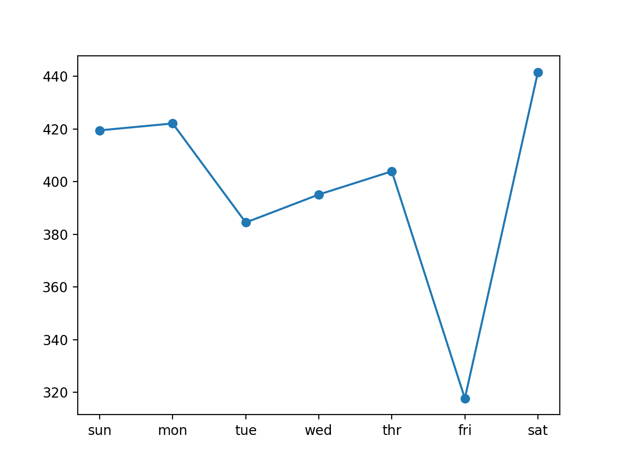
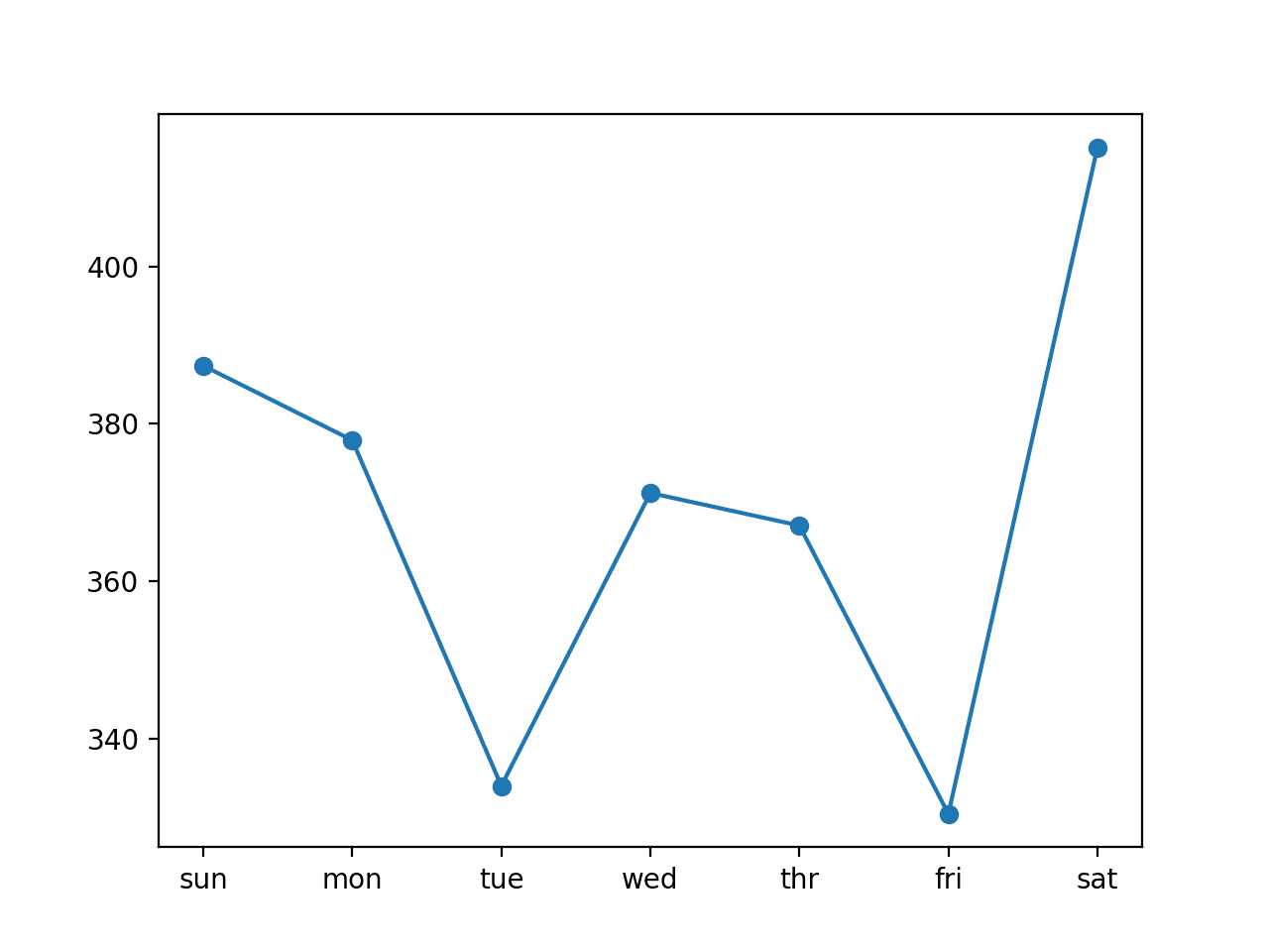
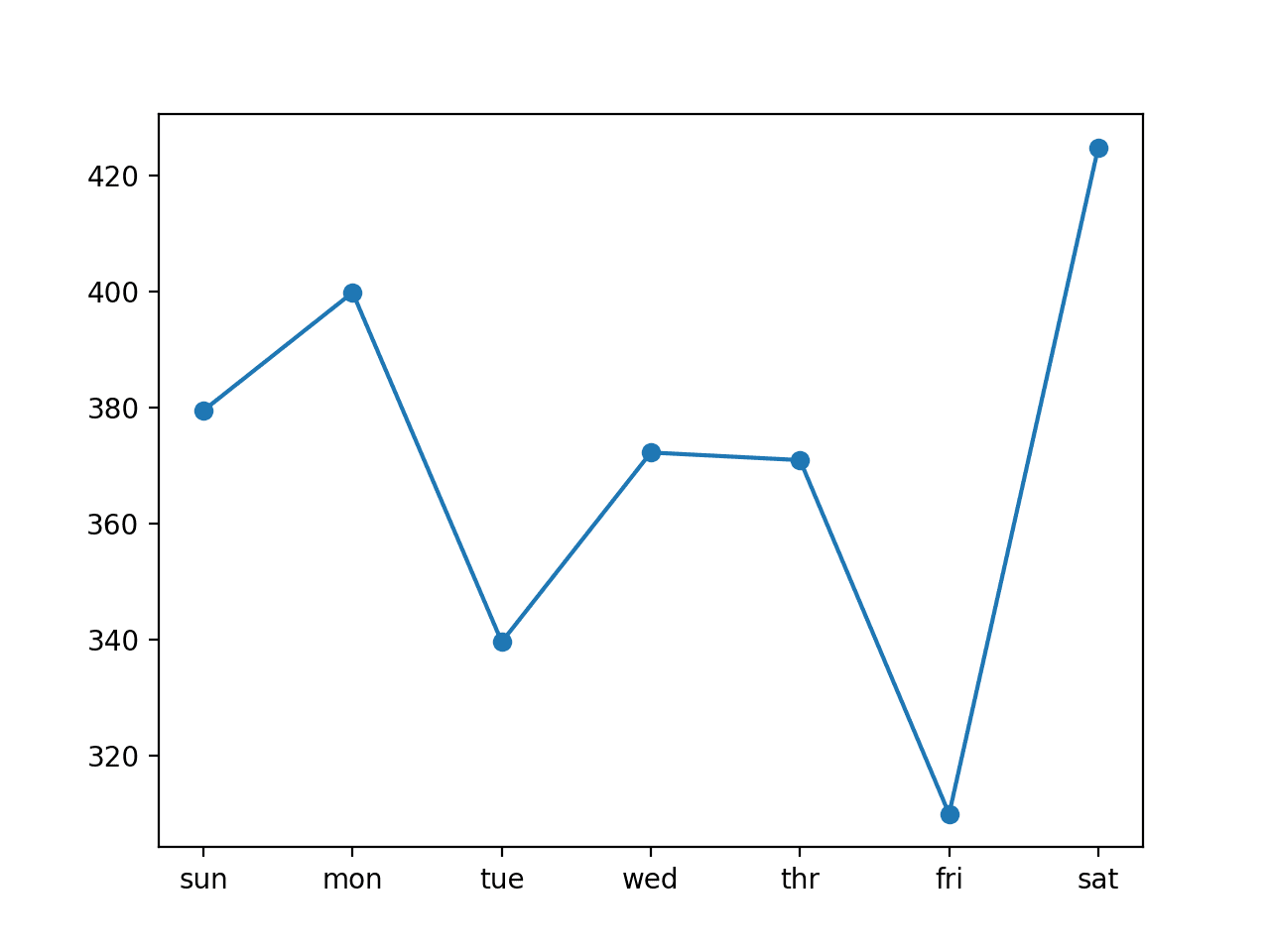
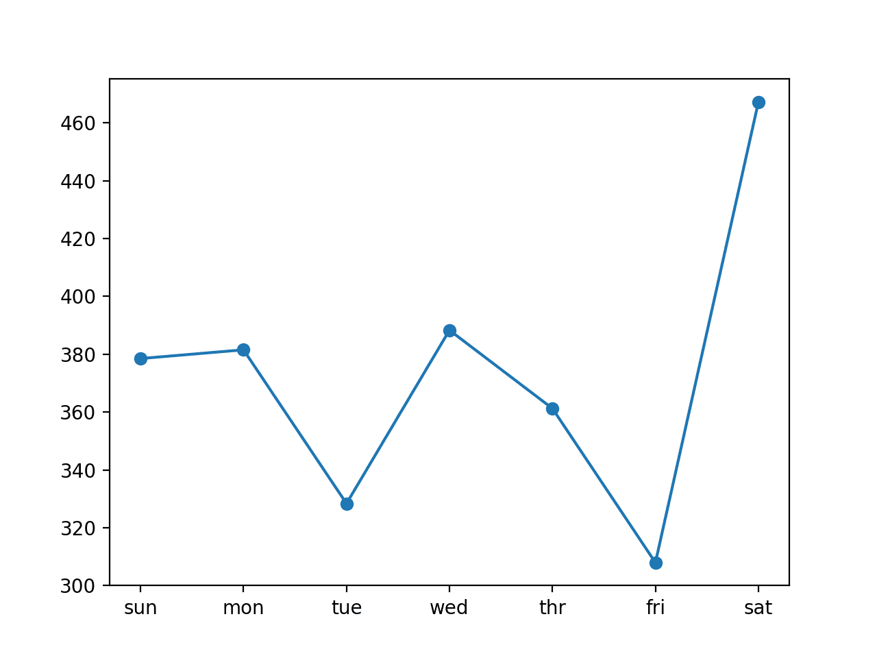
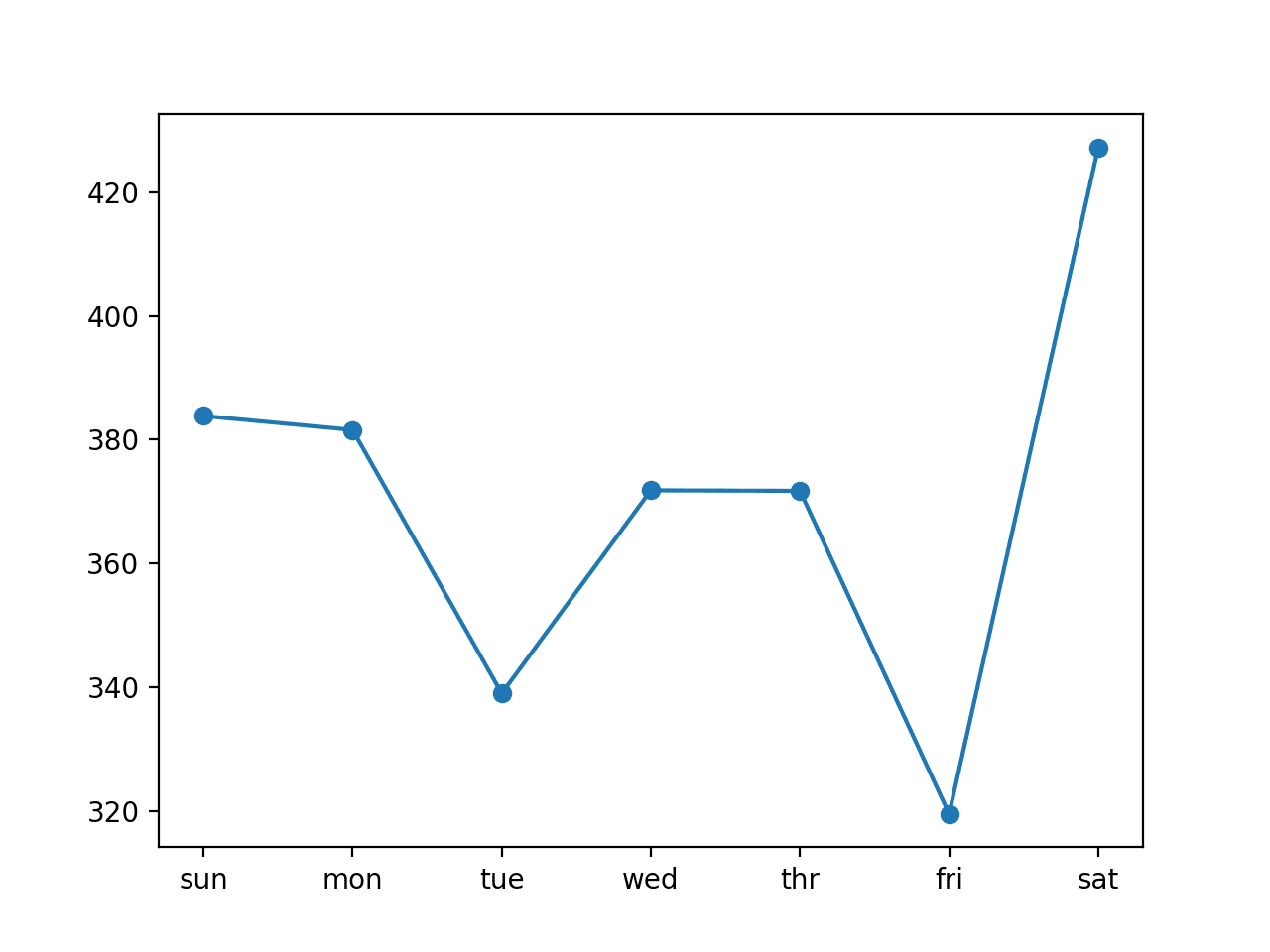
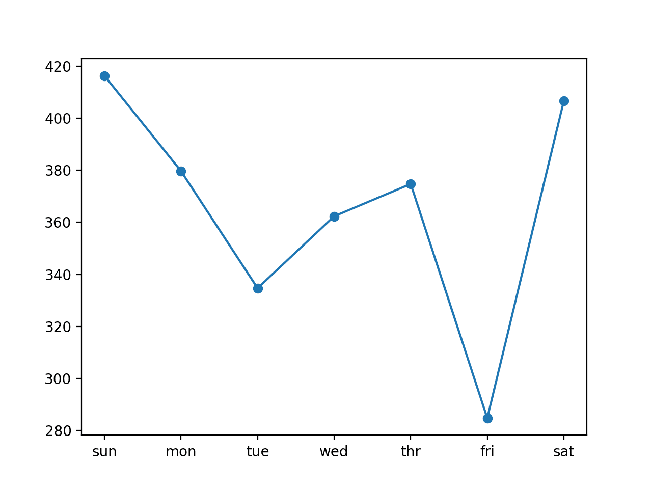


Hi Jason,
Thanks for another great article.
I’ve got a question about your thoughts about Attention based networks and how do they compere to LSTMs. I heard many voices in favor of the first ones, but I would like to know how this looks in real situations and not competitions-world 😉
Thanks,
Konrad
Attention-based models can offer a lot of benefit on challenging sequence prediction problems.
I have not used attention for time series forecasting though, sorry. Id on’t have good off the cuff advice.
Ok, sure, thanks for reply! 🙂
I ran the
Encoder-Decoder LSTM Model With Multivariate Input
and get the following results
lstm: [1566.582] 1611.0, 1526.1, 1515.5, 1596.3, 1494.1, 1504.0, 1707.5
which are significantly worse than the other approaches
What am I doing wrong?
# model.add(LSTM(200, activation=’relu’, input_shape=(n_timesteps, n_features)))
# model.add(Dense(100, activation=’relu’))
how do we choose LSTM unit and dense unit? for example, here 200 units for LSTM and 100 units for Dense have been used. is there any formula out there? should we guess?
it would be great if you could explain! Thanks in advance.
Trial and error. I explain more here:
https://machinelearningmastery.com/faq/single-faq/how-many-layers-and-nodes-do-i-need-in-my-neural-network
It is really hard to follow your explanations about the encoder decoder model. It does not say anything why this works as it looks like nromal LSTM models… I do not understand why you can use the normal training process to train such a model. I see very different training procedures, one with a normal fit statement and the other within a for loop:
https://blog.keras.io/a-ten-minute-introduction-to-sequence-to-sequence-learning-in-keras.html
https://www.tensorflow.org/tutorials/text/nmt_with_attention#training
Both saying they training via teacher forcing.
This is very confusing!
Perhaps start with the basics of LSTM and then progress to the encoder-decoder. You can start here:
https://machinelearningmastery.com/start-here/#lstm
Hey, I have difficulties to understand the difference in both training methods. Sometimes I use a for loop for training an encoder-decoder and sometimes like in your example, I use the fit statement.
Although you say that the decoder just predicts the next time step and not the output sequence (!) I would assume I would need to use also a for loop. So it is told that the decoder is trained for each output step, but then I do not use a for loop for iteration. That is confusing.
We use walk forward validation, perhaps this will help:
https://machinelearningmastery.com/backtest-machine-learning-models-time-series-forecasting/
No. I have issues with training. See here what I mean:
https://stackoverflow.com/questions/65291362/how-to-train-an-encoder-decoder-model/65295556#65295556
Also tzhis nice pytorch seq2seq tutorial!
https://pytorch.org/tutorials/intermediate/seq2seq_translation_tutorial.html
This implementation and via a for loop I can follow and understand. But where I have diffuclties to understand (what I wrote above) is why this is the same (?!) as training via a single fit statement (as in the keras blog and you did).
Maybe it is because it uses a different training data strcuture? Such that each example is just shifted 1 word? And this a single training example? Where training with a for loop I have as a single training example the wqhole sentnces (with all words)?
Sorry, I’m not sure how I can help/answer exactly.
Perhaps this will give you some insight:
https://machinelearningmastery.com/faq/single-faq/how-is-data-processed-by-an-lstm
Hi,
I think maybe my confusion is that tensrorflow has changed differently especially for RNNs the last time. I feel I have to learn everything new regaridng tensorflow and RNN! I lately see a lot RnnCells used for forecasting instead of training via a RNN layer. There, you also use a for loop. Oh my good, for loops are everywhere. But I think the follwoiing is not the same context?
Is this now everything the same? Or different usages for the same or indeed different methods for forecasting? Someone needs to write a blog to clarify the latest methods and usages for forecasting with tf.keras… 😉
https://www.tensorflow.org/tutorials/structured_data/time_series#multi-step_models
Is this model architecture the same as a encoder-decoder in the above article?
I’m not a fan of tf.keras, I still prefer standalone Keras:
https://machinelearningmastery.com/faq/single-faq/what-is-the-difference-between-keras-and-tf-keras
I recommend starting here:
https://machinelearningmastery.com/how-to-develop-lstm-models-for-time-series-forecasting/
How to calculate the accuracy of the Convolutional LSTM model of the electricity consumption dataset. Can you please provide the code for that?
It is a regression problem, we cannot calculate accuracy for a regression problem.
Is it possible to calculate accuracy with mse?
No, MSE is a calculation of error for regression.Accuracy is a calculation of performance for classification problems.
More details here:
https://machinelearningmastery.com/classification-versus-regression-in-machine-learning/
Hey Jason,
Great article. I’m trying to understand how you have your encoder decoder model vs. the official Keras example below:
https://blog.keras.io/a-ten-minute-introduction-to-sequence-to-sequence-learning-in-keras.html
I also worked through this example from JEddy92 where he adopted the Keras method to do time series analysis:
https://github.com/JEddy92/TimeSeries_Seq2Seq/blob/master/notebooks/TS_Seq2Seq_Intro.ipynb
I’ve tried building the Keras model as similar to your model as possible and running both over the same data. Your model seems significantly different from their example, and I can’t quite reconcile the differences.
I actually can’t get the Keras model for sequence to sequence to produce any good results for time series analysis. Running 1000 epochs and I got RMSE of 466.192. Have you built any time series models using the approach they are trying? Any ideas why this approach is so much harder to train than the one you have above?
I use a simple autoencoder LSTM approach which seems to perform better in my tests. The difference is learning an internal representation (autoencoder) vs copying state from the encoder. I explain the latter more here:
https://machinelearningmastery.com/develop-encoder-decoder-model-sequence-sequence-prediction-keras/
I don’t know about the post you’ve linked. I can report better performance in general with CNNs and hybrid models.
So you say other models performed better than LSTM.
Did you validate on same validation set (latest dates).
Yes.
This is a common finding, see this post:
https://machinelearningmastery.com/suitability-long-short-term-memory-networks-time-series-forecasting/
If i want to build a CNN -lstm model for forecasting and want to show accuracy what should i do !? I know it is a regression problem
Hi Troy…You may find the following resource helpful:
https://machinelearningmastery.com/cnn-long-short-term-memory-networks/
Multivariate prediction is which of these variables is predicted? I did not see the introduction of this part. Is the default giving the first variable of multiple variables?
Some of the models in the above tutorials take multivariate input and make a multi-step univariate prediction.
Hi Jason,
Great article, thanks.
I am trying out image (spectrogram) input sequences for classification output.
My network looks similar to “CNN-LSTM Encoder-Decoder Model With Univariate Input” with the difference that I am using TimeDistributed(Conv2D) layers and Multivariate Input.
Your examples do not use TimeDistributed Conv layers , but I was wondering if you have any thoughts ? My intention is to pass every sample of my batch individually through the Conv layer and collectively through the LSTM decoder. This I think would allow me to not have to explicitly preprocess my input data by collecting all samples representing a sequence together.
I am not sure if that would work okay, any comments would be a great help.
Thanks
You can adapt the above example to use a time distributed conv.
Perhaps try it and see, use results to guide you.
Hi Jason,
another great article, thank you… and this time it is exactly what I needed for my univariate time series forecasting project!
I learned so much from your tutorials and your book, I cannot be more grateful 🙂
I wanted to ask you a couple of questions, with reference to both proposed models (Vanilla LSTM and Encoder-Decoder):
1) If I wanted to make the (Vanilla LSTM / Encoder-Decoder) networks deeper, how should I insert more layers?
2) Statefulness, i.e., memory between batches: here you are using stateless networks, I guess you do that under the hypothesis that a single training batch contains all the series variability timescales we want to model, is that right?
If I wanted to make the models stateful to see if statefulness leads to better results with my series, how should I do that? I’m not sure in which layers I should set return_sequences = True.
Tank you very much for your attention, best,
Silvia
Thanks.
Yes, you can make a model deeper by adding more layers.
Don’t worry about statefulness for now, it does not impact model skill in my experiments.
Thank you for your prompt answer.
Now, it is very clear to me how I can add more layers in the Vanilla case, but not so clear in the Encoder-Decoder case. Should I add layers in both the encoder and the decoder? Could you please give me an example? Thank you for your patience, best, Silvia
You can add more layers to the encoder or more layers to the decoder.
Hi Jason, I am enjoying a lot these posts! I am trying to replicate the Encoder-Decoder LSTM Model With Multivariate Input, but instead of using daily data, I resampled the data to hourly values. The goal is to predict a full week of values at an hourly level.
I kept the rest of the model as is, except for the number of inputs (one week = 7*24) and the split_database, which now looks like this:
train, test = data[32:24392], data[24392:34472]
plt.plot(train)
plt.show()
# restructure into windows of weekly data
train = array(split(train, len(train)/(7*24)))
print(‘[samples(weeks), timesteps(hours), features]: {}’.format(train.shape))
test = array(split(test, len(test)/(7*24)))
print(‘[samples(weeks), timestemps(hours), features]: {}’.format(test.shape))
return train, test
When I train the RNN, I get nan values in the loss function from the very beginning.
I tried to use a MinMaxScaler on the data, and also tried with other optimizers, but I wasn’t successful.
Any insights on this matter? Thanks a lot 🙂
Perhaps double check your input data does not have any nan’s.
I did that, but there were no nans. I got it working using that MinMaxScaler, plus tanh activation functions instead of ReLu for the LSTM layers. Thanks a lot and keep up this awesome work you are doing.
Nice work.
Hi Daniel,
can show me your code? I don’t know where I have to rescale the data.
Thanks a lot and thank you Jason!
I show how to rescale data here:
https://machinelearningmastery.com/machine-learning-data-transforms-for-time-series-forecasting/
had the same problem. You need to convert the pandas dataframe to numpy array, then perform the split.
Hi Jason,
Thank you for the nice tutorial! It helps a lot! I noticed that you used differencing and scaling in the other tutorials for time series data, is there a reason why you don’t use it in this tutorial? Thank you!
To try to keep the example simple.
I do recommend scaling input and target variables in general. It will make life easier for the learning algorithm.
Hello Jason Brownlee,
You are one of my best research references, great job!
This article has helped me to understand something about the context, however, I have a question on how I can simulate or predict future values using machine learning or deep learning, but with algorithms and graphs showing clearly, for example, for a set of historical daily temperature data, how could I simulate a possible value for month 6 But 10 years ahead?
Do you have another article or link of any reference?
Thank you very much.
Rafael
Thanks Rafael.
The further into the future you forecast, the more error you can expect.
You could train a model to focus on predicting 10 years out.
Or you can use a short term model and run it out 10 years using outputs as inputs (e.g. recursive).
Perhaps this post will give you some ideas:
https://machinelearningmastery.com/multi-step-time-series-forecasting/
Hi, thanks for your very nice tutorial.
My question is about evaluating the overall RMSE during the training phase.
Is it correct to use this code:
from keras import backend as K
def root_mean_squared_error(y_true, y_pred):
return K.sqrt(K.mean(K.square(y_pred – y_true)))
and the use model.compile(optimizer = ‘adam’, loss = root_mean_squared_error ,metrics=[root_mean_squared_error])
instead of
model.compile(optimizer = ‘adam’, loss = ‘mse’)
I don’t recommend using RMSE for loss, instead I recommend using MSE for loss and RMSE as a metric.
I give an example here:
https://machinelearningmastery.com/custom-metrics-deep-learning-keras-python/
For the LSTM with multi-step forecasting, curious why you didn’t use LSTM layers with return_sequence=True and a Dense(1) output layer? Instead you have used two Dense layers, one with 100 outputs and an final Dense(7).
Would the return_sequence=True in an LSTM followed by a Dense(1) approach be wrong?
Note, we do use this approach in the encoder-decoder, which requires the use of a TimeDistributed wrapper layer.
Got it. So I take that to be a valid approach too?
Valid? I don’t follow, sorry.
Try a suite of models and the one that gives the best performance is the one to use. Whether a model works or not is not enough.
Hi, Great Article.
Should it not be “test” instead of “train” series?
Many thanks
No, here we are adding seeding the history with the training set.
Hi Jason,
Then won’t the first set of predictions be for the last of the training data?
If so, why are you passing the entire testing data for evaluate forecasts while ignoring the last of the training data that was used for seeding? Won’t this cause a problem?
Thanks.
We are using a process called walk-forward validation:
https://machinelearningmastery.com/backtest-machine-learning-models-time-series-forecasting/
You can adapt it for your own problem as needed.
I had the exact same question.
The code does not seem to use test_x anywhere.
It looks like train_x is used to predict test_y inside evaluate_model.
Are you sure this is correct?
Hi Jason! Any insights or rule of thumb to set input_size and batch size? Should these two be related?
Thanks a lot!
Unrelated.
Input size for lstms is the shape of each sample, e.g. timesteps and variables.
Batch size is the number of samples to process before estimating the error gradient and updating weights via backprop.
Thanks for your reply! So, if I am trying to forecast a full week with hourly granularity, and I have let’s say, a full year of hourly observations, would a large batch size better capture the variation in the dependencies accross variables in the past? Or would it depend only on the input size?
I would like the network to remember not only the recent behaviour, but also the past! 🙂
Thanks a lot!
Try it and see.
Hi again, I’d recomend anyone trying so to check out this paper, they give optimal hyperparameters for exactly the focus of this post using LSTM seq2seq 🙂
https://arxiv.org/pdf/1705.04378.pdf
Thanks for sharing.
Another thing worth mentioning when predicting several timesteps using LSTM seq2seq, for me it made a huge impact on the model learning to add L2 regularization rather than dropout, for those who see their model is overfitting! I got the idea from that paper!
Great tip. Yes, weight regularization is often overlooked and performs very well:
https://machinelearningmastery.com/weight-regularization-to-reduce-overfitting-of-deep-learning-models/
Hi Daniel, how did you apply L2 regularization in this case?
Is your code available on github?
Here’s an example:
https://machinelearningmastery.com/how-to-reduce-overfitting-in-deep-learning-with-weight-regularization/
I really like your Tutorial.
I am trying to improve the model by using forecast weather to improve the load forecast.
I have a dataset with many weather variables. I Want to build a model that use past_load, past_weather and future_weather to forecast future load.
I would like to know what is the best way to prepare the dataset to optimally use LSTM.
My problem is how to arrange the data in timesteps and features for each sample when there are some features that are not avalaible at all timesteps.
I have tested many approaches:
1) I have tried training my models with 1 timestep per sample and inputing all past weather and load and future weather as distinct features.
2) I also tried with many timesteps and one feature per time step but inputting a dummy value in the future load to make such that the model put zero weights in the future loads that will not be available when the model will be used in prediction mode.
I am sure that this is a common prediction problem and I am sure that there is a better way to proceed.
For missing data, you could try using a masking layer and mark the missing values to be ignored.
There is no best way in applied machine learning, I recommend testing a suite of framings of the problem in order to discover what works best for your specific dataset.
Hi,
Thanks for your article. I am working on crypto-price prediction, but I have lag in my predicting. I mean that my prediction is only based on my previous data, if price at t is 10 $, my prediction would also be 10 $, it means that at time t+1 we should expect the price to be 10 $; actually, I predict nothing. I have run your article’s code, and found that you may also have lag in your prediction. In addition, I have read your article about determining Base Line of predicting time series and I want to know what is the base line of house holds power consumption? is it greater than 370? can you explain more about LSTM lags?
It suggests that your model has learned a persistence model (e.g. has no skill).
I recommend experimenting with different methods and different framings of your data, including more lag observations (time steps) as input.
Thanks for your response, but still I think in this article your model learns nothing. It has 1-step lag and predict previous active power instead of predicting future. I think the base line of your model is not more than 370, and as you said in the other article, our model dose not learn any thing if we have RMSE more than base line.
They are skillful, but perhaps not the best you can achieve.
The LSTM models do better than than naive models:
https://machinelearningmastery.com/naive-methods-for-forecasting-household-electricity-consumption/
They also do better than linear models:
https://machinelearningmastery.com/how-to-develop-an-autoregression-forecast-model-for-household-electricity-consumption/
Hello!! Great Article.
I have a question Why your forecast model is different with this mentionned below:
https://machinelearningmastery.com/time-series-prediction-lstm-recurrent-neural-networks-python-keras/
Is it really depended of the dataset?
Thanks so much!!
Yes, models should suit the dataset.
Also, the post you linked to should not be used as a reference as the approach is pretty poor.
Thanks Jason for replying me!! I am new and interest into this domain LSTM. If i resume your program was to evaluate the model by calculating MSE and RMSE. How can i know exactly the total power will be consumed for example next Sunday or Friday?
In your code you use “yhat_sequence” which contains each week predict.
Is it this variable “yhat_sequence” we know the total power will be consumed?
Thanks
Yes.
To make a forecast,YOU retrieve last observations for input data.I don’t think that’s the right way to do it.Although this method is used in many papers and programs.
A more realistic way to reflect the performance of the model is as follows:
last 7 days of train data as input,forecast output next 7days,and then,use this output as next input,forcast another next 7days.we use recurring forecasts to get all 2010 Results.We compare the results with the whole test set,but no using the test data as input.
In this way, we can avoid leakage of time in the test data.
Thanks for your kind attention and look forward your prompt reply.
Yes, that is a common approach.
A preferred method is called walk-forward validation, you can learn more here:
https://machinelearningmastery.com/backtest-machine-learning-models-time-series-forecasting/
I want to achieve ConvLSTM Encoder-Decoder Model With Multivariate Input
and modify the source 2 functions as follow
8 means features
Nice work. Sorry, I don’t have the capacity to review your code changes.
model can be trained but forecast and evolution are failed.
Can you give me some advice?
What do you mean exactly?
# reshape into [samples, time steps, rows, cols, channels]
input_x = input_x.reshape((1, n_steps, 1, n_length, 8))
reshape function is failed.
ConvLSTM Encoder-Decoder Model With Multivariate(eg.8 features
) Input,I’m not sure about this model support Multivariate(eg.8 features
) Input.
Perhaps confirm that you worked through all steps and copied all code and that your environment is up to date.
Learning Diagnostics. Use diagnostics such as learning curves for the train and validation loss and mean squared error to help tune the structure and hyperparameters of a LSTM model.
Train dataset is splited into validation and train data.Validation sets are used to adjust loss.
Validation sets are not used a scheme called walk-forward validation.
test dataset will be used a scheme called walk-forward validation.
Is my understanding of this proposal correct?
Not quite. The train/test/validation split is challenging or may not even make sense when using walk-forward validation (e.g. sequence or time series data).
all code use this :mse = mean_squared_error(actual[:, i], predicted[:, i])
actual shape is 2d,predicted shape is 3d in some code.
I’m not sure whether this is correct
eg
predicted = array([[[1 ],
[2 ],
[3],
[4],
[5],
[6]],…
actual = array([[1, 2, 3, 4, 5, 6],….
Hi Jason,
Another great post, thank you!
I had a very general question: if my understanding is correct, these examples deal with splitting the data into train and test sets and then comparing the prediction with the test set with an RMSE. How do we make a prediction beyond the test set?
For example:
We train the model based on week 1 – week 9 data.
We pass the model a sample of week 10 data
How do we predict week 11?
In exactly the same way. e.g. model.predict()
Thanks for the prompt response! Just a quick follow up – if I were to separate the training phase by saving the model and then performing predictions later on – would I still require the full history of the train data?
Reason being, I notice that when calling evaluate_model you are not only training the model with the training data but also using it as history:
history = [x for x in train]
Does that imply that I would need the full training set data again for the prediction phase? or is it enough to just use new test data as history and run against predictions against the saved model?
Only enough history to make a prediction is required.
Hi Jason, great post. I have a question related to James’ above.
If I call model.predict() using the final week (e.g., Week 10) of my testing set as input data, I am predicting Week 11 values, not Week 10 values, correct?
Thanks again
Yes. Remember it is just a model with inputs and outputs:
https://machinelearningmastery.com/how-machine-learning-algorithms-work/
Thanks Jason.
I wonder, do you have a simpler example focusing only on the multi-step forecasting? This would be very helpful, since I’m only interested in that at the moment.
Yes, I have a simple example here:
https://machinelearningmastery.com/how-to-develop-lstm-models-for-time-series-forecasting/
If you have multiple features predicting some dependent variable different from those features, meaning can you think of each time-step of these features as a sequence? That is, assuming each row is a time step and each column a feature (and that all features are normalized, Z-scored), does it make sense to use a plain LSTM on this sequence, even though the sequence is not temporal?
Sorry, I don’t follow your problem definition, perhaps you can elaborate it?
Let’s say I am predicting US stock market (my Y) by looking at time series features such as UK and German stock market (X1 and X2). So, with 2 features, and let’s say the last week of time values, your Keras input would be (samples, 7, 2) in shape. Is this inherently better than just using X1 and X2 at the current time step to predict Y? That is, using (X1, X2) to predict Y in a way where input would be (samples,seq length = 2, channels = 1). Does this ever depend on the specific domain as well? To me, it makes sense that past values have a particular ‘pattern’ that correlates with future values. If you, on the other hand, combine X1 and X2 together, you are looking for a pattern/correlation *across* the features that determines the value. I have seen situations where the same problem has been tackled both ways, but I wonder if one is more likely to be successful than another
It depends on the specific of the problem.
Also, in general, LSTMs are terrible at time series forecasting compared to other methods.
Is the result of the model a single training or an average of multiple training in this post?
In general, model weights are updated at the end of each batch, there are many batches in each epoch and we fit for many epochs.
The small batch size and the stochastic nature of the algorithm means that the same model will learn a slightly different mapping of inputs to outputs each time it is trained. This means results may vary when the model is evaluated.
Your results is an average of model performance?
You can reduce the variance of the model by fitting the model many times and averaging the performance.
That is not done in this tutorial.
Hi Jason, can you clarify how to evaluate multiple step forecasting, like the mathematical formular behind. In this case, it is 7 steps forecasting, so is the formular sum( sqrt(mse(t1)+mse(t2)+…+mse(t7)), sqrt(mse(t8)+…+mse(t14)), ….)? ti is the difference between predicted and actual for time I.
You can evaluate each forecasted lead time separately, or combine all lead times and calculate a single error measure.
I recommend the former approach and that is the approach used in this tutorial.
Thank you for your reply. How can we choose the model using this approach? There may be some cases when model 1 has lower Error for Monday to Wednesday and model 2 has lower error for Thursday to Saturday.
Same thing.
If you can achieve lower overall error using a mixture of predictions of different models, then that is your “model”.
Thank you so much! It sounds like an ensemble method.
No, you can achieve this with one model. You can achieve it with a direct model for each forecast lead time, and I show this in another tutorial:
https://machinelearningmastery.com/multi-step-time-series-forecasting-with-machine-learning-models-for-household-electricity-consumption/
Say I’m interested in predicting the probability distribution of household power consumption in the following 1-day period, so is there any methods that can predict the probability distribution? If so, how would you evaluate accuracy of these stochastic predictions?
Probability refers to an event, what is the event? Usage above a threshold?
If in that case, it is a 2d probability distribution. A start would be probability per time interval and use a metric for comparing distributions per interval, like kl divergence.
Please let me clarify the question a bit. The models you developed in the tutorial are dealing with mean predictions, i.e. one prediction for one time step ( the model may predict the consumption would be 500 for tomorrow). The result (500 consumption) is a mean prediction because the consumption has the stochastic nature (50% chance to be 450 and 50% chance to be 550). Is there any ways to analyze this stochastic natural or the probability distribution of each possible consumption outcome?
Not quite. One model will make one deterministic forecast for each day.
For a range of forecasts for each day, an ensemble (e.g. a bootstrap) of models is required from which a distribution could be estimated and interpreted as a prediction uncertainty.
In other words, if the model predicts 500 for tomorrow, then is there any ways to evaluate the likelihood to be 500 for tomorrow and the probability for other possible outcomes?
Yes, this is called a prediction interval:
https://machinelearningmastery.com/prediction-intervals-for-machine-learning/
An ensemble of models sounds like a great idea to approximate a distribution for a range of forecasts. Then can we evaluate the accuracy by using kl divergence to compare predicted distribution and empirical distribution from the dataset?
Do you think poisson distribution can possibly be used to approximate the distribution for power consumption?
These are separate ideas, I don’t think they mix. E.g. prediction intervals and predicting a probability. A prediction interval is not a predicted probability of an event, it is the scope of uncertainty of a point prediction.
I recommend reading some of the background material I’ve posted and perhaps start with a strong definition of what you want to model:
https://machinelearningmastery.com/how-to-define-your-machine-learning-problem/
Sorry for the confusion. I referred to predicting probability distribution for all possible outcomes in the next time interval, not a prediction interval.
The model cannot do this, as stated.
Right. I am going to try ensemble method and poisson distribution to do this. Thank you very much! It’s very helpful.
Encoder-Decoder Model,
Encoder plays import role or Decoder Model does?
ConvLSTM Encoder-Decoder Model,LSTM may plays import role
Does Encoder play a role in extracting features?
It extracts features from the encoding.
Hi, Great Tutorial ! Thanks alot for doing this.
I have a question. can you please explain me what is the evaluate forecast function doing?
Is it calculating the rmse for all the days of all the weeks or just the last week predicted?
Also are the ‘scores’ of just the last week predicted? because they are 7 in number.
It is calculating the RMSE for each day in weekly forecast.
Hi Jason,
I have question, If I have 3 features (A,B,C) and I can access the future information from 2 of them (B,C). how can I predict A feature for multi step ahead ? how does the input array looks like for RNN LSTM ? what is the best framing problem for this situation ?
Maybe this will help:
https://machinelearningmastery.com/faq/single-faq/what-is-the-difference-between-samples-timesteps-and-features-for-lstm-input
Thanks Jason, do you have experience with LSTM in NARX or something like A Dual-Stage Attention-Based Recurrent Neural Network for Time Series Prediction ?
No, sorry.
Hi Jason. Thanks for your amazing tutorials. I have already read almost all article about this topic, but I’m trying to implement an LSTM model to make binary (or multiclass) classification from raw log data(Raw Mooc courses log data -> user-level droput/grade prediction ).
Sample from data: https://bit.ly/2SiPcjG
I have read lots of publication and tutorials which seems to be what I’m looking for, but couldn’t find any example on how to use it.
My biggest challenge to making a prediction for unique users, and feed the network with a user-level dataset.
Do you have any idea?
I have an example here:
https://machinelearningmastery.com/how-to-develop-rnn-models-for-human-activity-recognition-time-series-classification/
Hello Mr Brownlee
I have to implement a multi-step forecasting project and i m really confused, so i would appriciate if you could help me.
I have a lot of papers and for each paper a sequence of citations per year.
Let say for example :
paper1 : (2000,1), (2002, 2), (2008, 3), (2011, 4), (2012, 5)
paper2: (1990,3), (2003,1), (2015,4)
.
.
.
paperN: (2007,3)
My goal is to predict the paper’s citation in the next year(let say t+1) and also in 5 years later(let say t+5) depending on the previous years citations.
Which model is more suitable?
Is it an autoregression prooblem?
How do i deal with the different length of the sequences? Should i pad the sequences with zeros ?
Also each sequence corresponds to a different paper.
Any ideas or suggestions?
Thanks in advance!
I recommend following this process:
https://machinelearningmastery.com/how-to-develop-a-skilful-time-series-forecasting-model/
These tutorials may help:
https://machinelearningmastery.com/start-here/#deep_learning_time_series
Jason,
Great tutorial.I’m trying to understand if a ConvLSTM Encoder-Decoder Model but with multivariate Input is the best model for my dataset.
I have a simplified plasma simulation which has around 22,000 timesteps of data. For each timestep the plasma parameters are recorded at one of 200 locations, and at each location 12 different variables are recorded. The 12 variables are a function of each other and a function of their location.
I have created the dataset so it is a 2D array of appended matrices so that for each variable, you have the spatial data of the 200 locations. i.e. Var1-Loc(0,1,2…198,199), Var2-Loc(0,1,2…198,199)….. Var12-Loc(0,1,2…198,199).
So the 2D dataset is 2400 columns (12 variables @ 200 locations) with 22,000 rows
There is a need to train the neural network and predict how the plasma will behave n-timesteps into the future. Would a ConvLSTM Encoder-Decoder Model With Multivariate Input be the best architecture to go for or do you suggest an alternative architecture?
Cheers
Peter
Generally, my advice would be to test a suite of models/framings of the problem and discover what works best.
It does sound like a convlstm is a good fit though.
Let me know how you go.
Hello Jason,
Which function to change if i want to predict one step.
# split a univariate dataset into train/test sets
def split_dataset(data):
# split into standard weeks
train, test = data[1:-328], data[-328:-6]
# restructure into windows of weekly data
train = array(split(train, len(train)/1))
test = array(split(test, len(test)/1))
return train, test
This is a large change and would require modification of both the preparation of the dataset and the model.
Perhaps start here:
https://machinelearningmastery.com/how-to-develop-lstm-models-for-time-series-forecasting/
Thanks Dr. Jason for your reply.
Love it, saved my final year thesis!
It would however be nice with a tutorial on how to actually use the trained model to predict on new data and how to display the results in a useful way. By useful I mainly think of plotting the known data and the predicted data in a plot with dates (or time in general) on the x-axis.
Yout site and email courses have been gold trying to learn this stuff! Keep it up!
Thanks.
I show how to make predictions here:
https://machinelearningmastery.com/how-to-make-classification-and-regression-predictions-for-deep-learning-models-in-keras/
And here:
https://machinelearningmastery.com/make-predictions-long-short-term-memory-models-keras/
I hope that helps.
Hey Jason – how would the CNN LSTM extend to multiple input time series & predicting multiple output time series features? Is it as simple as reshaping the Y to
# reshape output into [samples, timesteps, features]
train_y = train_y.reshape((train_y.shape[0], train_y.shape[1], n_features))
and changing the final layer of the network:
model.add(TimeDistributed(Dense(n_features)))
Or do you also need to change the structure of the initial convolutional layers?
Cheers
Jack
I have a few examples, perhaps start with this post:
https://machinelearningmastery.com/how-to-develop-lstm-models-for-time-series-forecasting/
Hey Jason,
In the example Encoder-Decoder LSTM Model With Multivariate Input, I would like to know the model takes in multivariate input and predicts which feature and where is it specified in the code. I assume that it predicts the 1st input feature correct me if I am wrong.
Thanks
Yes, it is in the name of the section:
“7. Encoder-Decoder LSTM Model With Multivariate Input”
Perhaps re-read the tutorial?
Walk-Forward Validation in this post,how to develop the model and tune the model ?
Thanks!
See this post on how to tune a model:
https://machinelearningmastery.com/how-to-grid-search-deep-learning-models-for-time-series-forecasting/
Hi Jason,
Thanks for your post! I tried multivariate input for the CNN-LSTM and ConvLSTM model. I took the average of 100 iterations and compared with univariate input case. It looks like multivariate input does not improve the forecast a lot. Maybe it’s because I haven’t tune the model yet. So my general question is that: Does more input variables always result in a better forecast?
Thanks
Well done!
No, it really depends on the specifics of the dataset and model.
Thanks so much for this tutorial!
I would like to predict some image characteristics such as size, position, etc.. based on search-keywords.
I have a csv where for each keyword, image characteristics are given (training data). For instance:
Keyword X0 Y0 Xn Yn Width Height position ImgID
cat 261 49 872 690 611 283 top 2
cat 23 43 866 565 603 270 buttom 3
What lstm model best fit with such task?
It can be considered as time series problem?
Thank you
jezia
It looks like a regression problem, but not a time series prediction problem.
Perhaps try an MLP?
Can you tell, how well your model is performing in terms of MAPE?
Good question.
You can calculate MAPE using the ‘mean_absolute_percentage_error’ metric, I given an example here:
https://machinelearningmastery.com/custom-metrics-deep-learning-keras-python/
Hi,Jason:
In this case, why dont u use the normalization to processing the dataset?I found the loss is very big when i traing the networks.
Thanks for u reply!
Yes, it is a good idea to normalize the input and output data prior to modeling.
I left out that step of data preparation to focus on the modeling part of the tutorial. In other tutorials when I included data prep, more people were confused.
Thank u, Jason.
I normalized the input and got the ideal loss, but I want to do the inverse normalization when calculating rmse, but the calculation is still the normalized value, maybe you can give me some advice.
You can use the inverse_transform() on the scikit-learn encoder object.
I defined this in the code assignment phase:
scaler= preprocessing.MinMaxScaler()
dataset = scaler.fit_transform(dataset.values)
train, test = split_dataset(dataset)
But I don’t know where to use the inverse_transform() to make the training process use normalized values, but to calculate the RMSE using actual values.
No problem, I show how here:
https://machinelearningmastery.com/machine-learning-data-transforms-for-time-series-forecasting/
@Jc.zhu did you get where to put the inverse_transform()
I too am struggling with this. I think the inverse_transform would be placed in the function “evaluate_forecasts” but I haven’t worked out the right way to apply it. As I understand it, the whole matrix that was initially passed into the “fit_transform” function needs to be passed. Not sure how to do that when it seems we are chunking only part of the matrix through the “evaluate_forecasts” function. Anyone figured this one out???
Thanks,
Nick
See this re transforms and inverse transforms:
https://machinelearningmastery.com/machine-learning-data-transforms-for-time-series-forecasting/
Hi Jason,
Thanks for your post!
I would like to know how to obtain the internal representation values of the last model (ConvLSTM Encoder-Decoder Model With Univariate Input).
Thanks again.
Sha
You could use the functional API and define the bottleneck layer as one of the output layers?
This post will give you ideas:
https://machinelearningmastery.com/lstm-autoencoders/
Thank you for the tutorial.
I have a domain-related question. How reasonable is it to sum the power values over 1-day periods? It is like you measure your velocity every minute (80 mph, 75 mph, 85 mph…) then you sum all those up to say you have a velocity of ~24 * 60 * 80 mph for that day. It doesn’t make sense physically but it may not be affecting the forecasting accuracy. If we definitely want to downsample to daily intervals it should be for energy, not power (you can indeed sum up distance covered, but not velocity).
I’m not sure I follow, sorry.
Hi Jason
Thanks for your tutorial, it helps a lot.
I want to stack two ConvLSTM, that means replace LSTM with ConvLSTM. For example time_step is 3 like input [10,3,25,25,1] and output is [10,3,2]
The question is on this part model.add(RepeatVector(n_outputs)) when I set n_outputs = 3 as time step, I got error that convlstm expect ndim = 5, found ndim = 3
What will be the problem base on your experience because we need the encoded output to be repeated the same number of time_step
I’m not sure the convlstm and be used directly in the encoder-decoder, some changes to the model may be required. I don’t have an example, you may have to prototype a few approaches.
Hello Jason,
I am adapting your last section code of this post to predict trajectories, so I need an output such as (1,18,2). The 18 is because I am predicting 18 times ahead and 2 is because I am predicting x,y.
How can I adapt the model to have that output? Currently I am having this error:
ValueError: Error when checking target: expected time_distributed_2 to have shape (18, 1) but got array with shape (18, 2)
By the way, your posts are amazing. Thanks very much for create them 😀
My best advice is to start here to work through how to apply models like this to your dataset:
https://machinelearningmastery.com/start-here/#deep_learning_time_series
Hello Jason,
Thanks very much for your advice, it was very helpful 😀
You’re welcome, happy to hear that.
Hi Jason,
Congrats for the blog, it is great and really useful.
I am trying to do a multi-step prediction of a continuous signal. Based on the past 100 samples of the signal I try to predict the next 10. It is univariate input and output but multi-step prediction. I used the model you propose in the “Encoder-Decoder LSTM Model With Univariate Input” section.
My results are a bit curious as I observe that the first 2 or three immediate samples have a higher error than the rest. Basically, it is more difficult for the network to guess what is going to happen on the next second than 3 seconds from now. Do you by chance have any clue of what can be happening? Maybe I am not using the right approach/model?
Thank you!
Perhaps try a suite of different models in order to see what works best for your specific dataset.
This process may be helpful:
https://machinelearningmastery.com/how-to-develop-a-skilful-time-series-forecasting-model/
Thank you! I changed the activation functions and the optimizer and it worked.
I have yet another question. Is it possible to predict two features at the same time? What I mean is that my output vector Y would have the shape Y(samples, timesteps, 2). Would that be possible? I could not find any example in your blog and neither in a quick search in Google and I was wondering if that is possible at all or you should use the same model twice for each of the features that you would like to predict.
Thanks again. 🙂
Yes, the model would output a vector, one value for each feature, and an encoder-decoder can output multiple time steps for each feature.
This post has an example I believe:
https://machinelearningmastery.com/how-to-develop-lstm-models-for-time-series-forecasting/
In to_supervised function the output array dimensions were X=[1099, 7, 1] and y=[1099, 7].
Why it can’t be the same.
when we fit the model does it take if we make the dimension of array y same as X?
The model output must be one vector for each sample.
The output may be 3d in the case of using an encoder-decoder model.
1. Does it remember the past pattern (long ago) to impact on the present prediction in the vector model?
2. I want to use this model for web app when I give my data by choosing 1 st time 12 output value, again I’m giving the same data choosing 24 output, that time previous model values existed in present model? Whether it works?
It can, if required.
I recommend testing it to discover whether it works for your specific dataset.
Is it possible to find prediction intervals also with LSTM model?
Hmmm, yes there are methods for neural nets, I believe I link to them here:
https://machinelearningmastery.com/prediction-intervals-for-machine-learning/
Hi Jason,
Any reason for this well-known problem in timeseries forescasting using LSTM’s? 1-step lagged predictions. See below:
https://stackoverflow.com/questions/52778922/stock-prediction-gru-model-predicting-same-given-values-instead-of-future-stoc
I’m trying to do multivariate input for predicting univariate 1-step in the future, using LSTM, and I’m facing this problem of shifted predictions. Any light on this problem would be awesome.
Great job on this website, congrats. I’m buying your book on Deep Learning for Time Series forescasting now 🙂
Yes, it suggests the model has learned a persistence model, learn more here:
https://machinelearningmastery.com/faq/single-faq/why-is-my-forecasted-time-series-right-behind-the-actual-time-series
Thanks. I’ll try to solve it.
I’m training a LSTM with multiple sequences of 100 time steps (t-100, t-99, …, t ) for 8 sensor measurements (multivariate time series). Then I try to predict for t+1 the value of one of the 8 sensors (and then the problem of shifting happens).
Do you think there is any model more suitable for doing accurate predictions, rather than using LSTM for this kind of problems? maybe CNN-LSTM? I have bought your book but I’d like to focus on the most promising techniques for modelling this problem as best as possible. I’d thank any help to focus the search throught your book.
Thanks Jason!
I have had good success with CNNs and CNN-LSTMs.
Nevertheless, I’d recommend starting with a naive method, then a linear method, then try a suite of neural nets in order to discover what works well/best.
I understand.
Please, could you give me a few names of promising algorithms for my specific problem of time series forecasting that support multivariate data?
Deep Learning: CNN, CNN-LSTM
Others for neural nets or classical ones?
Thanks
Yes, I’d recommend starting with this process:
https://machinelearningmastery.com/how-to-develop-a-skilful-time-series-forecasting-model/
Some more classical methods here:
https://machinelearningmastery.com/time-series-forecasting-methods-in-python-cheat-sheet/
Thanks Jason.
I was wondering if classical methods handle these kind of problems:
1 – multivariate input – univariate one-step forecasting
2 – multivariate input – univariate multi-step forecasting
If not, I guess I should be directly using CNN-LSTM or CNN….isn’t it?
Yes, perhaps NAR/NARIMA/etc, not sure if statsmodels supports them though.
Start with a univariate model and compare all performance to it to determine if you have a lift in skill.
how can we extract the predicted values for the corresponding actual values for the week?
Not sure I follow, what is the problem exactly?
You can make a prediction via: model.predict(), more here:
https://machinelearningmastery.com/make-predictions-long-short-term-memory-models-keras/
# plot scores
days = [‘sun’, ‘mon’, ‘tue’, ‘wed’, ‘thr’, ‘fri’, ‘sat’]
pyplot.plot(days, scores, marker=’o’, label=’lstm’)
pyplot.show()
the above code snippet is for which week? can you please provide the dates instead of the days in the plot?
In that case we are plotting the average error on each forecasted day, not a specific forecast.
I recommend this much simpler tutorial first:
https://machinelearningmastery.com/how-to-develop-lstm-models-for-time-series-forecasting/
why whenever i use lstm it’s display “using tensorflow backend ” error , i was search and don’t find any solutionز
That is not an error, it is an information message.
Learned a lot of things today. Want to try out on stock prices.
Thanks.
Perhaps not stock prices though, they’re not predictable.
hello,
every time i run the model i get different predicted values. How can i get consistent values?
I added theses lines at the starting of my code, but the problem still persists
from numpy.random import seed
seed(2)
from tensorflow import set_random_seed, random_uniform
set_random_seed(2)
Good question, the best approach is to fit multiple models and average their results, more here:
https://machinelearningmastery.com/ensemble-methods-for-deep-learning-neural-networks/
Hello,
I’m trying to use the ConvLSTM Encoder-Decoder in order to encode and decode a 8 hz time series dataset but I’m completely confused with input_shape. At the beginning I have a dataset of 1219810 rows and 8 colums. I decided to reshape it with 121981 samples of 10 rows and 8 colums. How should I reshape my data for the ConvLSTM model then ? I tried to do data.reshape(121981, 1, 10, 8, 1) but that returned that the timedistributed layer does not expect this shape. I read the article but I’m too confused to adapt it to my dataset
I would really appreciate some help ! Thanks !
Perhaps you can use the above example as a starting point, then adapt it for your specific dataset?
HI Jason
Do have the solution to the same problem in R.
How to Develop LSTM Models for Multi-Step Time Series Forecasting of Household Power Consumption in which you solve the problem using R. Thanks
Sorry, I don’t have examples of time series in R. I may cover the topic in the future.
hi jason, if i want to forecast 30 days ahead based your code, the final dense must 30?
Yes, or you can use a recursive model:
https://machinelearningmastery.com/multi-step-time-series-forecasting/
Hi Jason,
In the text you mention that we need to iterate over the time steps and divide the data into overlapping windows for training the neural network. You basically have a input-output pair, feed it to the neural network, move one day ahead so that the first value that was previously in the output list, will now be the last value in the input list and add another unseen value to the output list. There will be scenarios where the input list is the same as the output list, 7 steps back. Won’t this cause the leakage of data? You are using input that the neural network has already seen, namely as output.
It seems to fit the description you use of data leakage pretty well, as seen here:
https://machinelearningmastery.com/data-leakage-machine-learning/
It really depends on how you frame the problem and what you want to test.
What we have described here is called walk-forward validation:
https://machinelearningmastery.com/backtest-machine-learning-models-time-series-forecasting/
Hey Jason, Thank you so much for these posts I really love them and rely on them.
Thanks, I’m glad they help.
Hello Jason,
I found this type of error.
I would like to make a forecast in minutes
Using TensorFlow backend.
[samples(weeks), timesteps(minutes), features]: (36, 10080, 1)
[samples(weeks), timestemps(minutes), features]: (5, 10080, 1)
(36, 10080, 1)
(5, 10080, 1)
Traceback (most recent call last):
File “C:\Users\Desktop\Learning.py”, line 149, in
model = build_model(train, n_input)
File “C:\Users\Desktop\Learning.py”, line 74, in build_model
train_x, train_y = to_supervised(train, n_input)
File “C:\Users\Desktop\Learning.py”, line 69, in to_supervised
return array(X), array(y)
MemoryError
I need your advise!
Sorry to hear that.
Perhaps try using less data?
Perhaps try running on a different machine?
Dear Dr. Jason:
I’m a big fan of you, and I’m very interested in your LSTM research. When I run # univariate multi-step lstm, I set up the Python 3 running environment according to your instructions. What’s the matter? I need your help! Thank you!
Traceback (most recent call last):
File “D:\Deep Learning\PyCharm 2017.2.3\helpers\pydev\pydev_run_in_console.py”, line 78, in
globals = run_file(file, None, None)
File “D:\Deep Learning\PyCharm 2017.2.3\helpers\pydev\pydev_run_in_console.py”, line 35, in run_file
pydev_imports.execfile(file, globals, locals) # execute the script
File “D:\Deep Learning\PyCharm 2017.2.3\helpers\pydev\_pydev_imps\_pydev_execfile.py”, line 18, in execfile
exec(compile(contents+”\n”, file, ‘exec’), glob, loc)
File “D:/univariate multi-step lstm.py”, line 6, in
from sklearn.metrics import mean_squared_error
File “D:\Deep Learning\PyCharm 2017.2.3\helpers\pydev\_pydev_bundle\pydev_import_hook.py”, line 21, in do_import
module = self._system_import(name, *args, **kwargs)
File “E:\anaconda3-4.4.0\envs\dlwin36\lib\sklearn\metrics\__init__.py”, line 7, in
from .ranking import auc
File “D:\Deep Learning\PyCharm 2017.2.3\helpers\pydev\_pydev_bundle\pydev_import_hook.py”, line 21, in do_import
module = self._system_import(name, *args, **kwargs)
File “E:\anaconda3-4.4.0\envs\dlwin36\lib\sklearn\metrics\ranking.py”, line 29, in
from ..utils.multiclass import type_of_target
File “D:\Deep Learning\PyCharm 2017.2.3\helpers\pydev\_pydev_bundle\pydev_import_hook.py”, line 21, in do_import
module = self._system_import(name, *args, **kwargs)
File “E:\anaconda3-4.4.0\envs\dlwin36\lib\sklearn\utils\multiclass.py”, line 21, in
from ..externals.six import string_types
ImportError: cannot import name ‘string_types’
Sorry to hear that, perhaps your environment needs to be updated:
https://machinelearningmastery.com/setup-python-environment-machine-learning-deep-learning-anaconda/
After some hard work, I succeeded in running out, thank you very much!!
Well done.
There’s one (well there’s many but mainly one) part that’s confusing me a bit…
In the walk forward validation in the evaluate_forecast function.
What if we have only one week of test data, would this still give valid predictions? Wouldn’t that mean that the predictions are based only on the data from the training set used for seeding?
I’ve followed this tutorial and applied to a problem to predict two hours ahead based on the last 24 hours of power consumption. But this part is giving me a headache…
Yes.
Historic or lag obs are used as input to make a forecast.
For more on walk-forward validation, perhaps this will help:
https://machinelearningmastery.com/backtest-machine-learning-models-time-series-forecasting/
Hi Jason and thanks for the awesome tutorial.
I must tell you that the code does not work due to using the
splitnumpy function in thesplit_datasetfunction.It returns
array split does not result in an equal division.I tried to use the
np.array_spltwhich is ok but then we have a problem at thedata = train.reshape((train.shape[0]*train.shape[1], train.shape[2]))line inside theto_supervisedfunction.It returns
tuple index out of rangebecause train has just one dimension.If you change it to
data = train.reshape((train.shape[0], 1)), it returns:setting an array element with a sequencewhen calling fit method(For the above last error message, take into account that I have tested it with tensorflow2.0 api , so I am not sure if with 1 has a problem)
Also, if we have enough weeks (not 159 as you say, but 800 for example) , at the
to_supervisedfunction can we use instead the version with the shit?Like:
def to_supervised(input_arr, shift=1):
df = pd.DataFrame(input_arr)
columns = [df.shift(i) for i in range(1, shift + 1)]
columns.append(df)
df = pd.concat(columns, axis=1)
df.fillna(0, inplace=True)
values = df.values
X, y = values[:, 0], values[:, 1]
X = np.expand_dims(X, axis = 1)
return X, y
and use these X,y inputs in the build model?
Thanks!
George
Sorry to hear that you are having trouble running the code, I have some suggestions for you here:
https://machinelearningmastery.com/faq/single-faq/why-does-the-code-in-the-tutorial-not-work-for-me
Jason , I was wrong!
I just saw that you are using the consumption_days.csv and not the consumption.csv.
I didn’t notice that, sorry.
You can ignore my previous message expect from the last part where I ask if we can somehow use the shift function .
Thanks!
George
No problem.
Jason,
Thank you for putting these amazing tutorials together. I really appreciate the effort you put in to make various machine learning techniques understandable.
I’m trying to understand the difference between your model architecture and the one presented in (https://blog.keras.io/a-ten-minute-introduction-to-sequence-to-sequence-learning-in-keras.html). Is the main difference that you know the number of steps you are trying to predict out is fixed. Whereas, in the Keras blog this would work for a variable output length?
Yes, the Keras blog uses a dynamic RNN, whereas I typically use a fixed length input/output as it greatly simplifies the code.
So I want to jump on this thread. Can’t that be fixed with changing the number of state that are returned with the ‘Repeat_Vector(n)’ layer? For instance, input of 100 timesteps with output of 5 timesteps. Input would have shape (100, features) for your input layer, and next layer would be Repeat_Vector(5). Say you wanted to do 10 timesteps in the future next, then you just change 5 to 10 in the Repeat_Vector layer?
Or am I missing something?
Yep.
Hi Jason!
I wanted to ask you.
If I use the metrics ‘mae’ and ‘mape’ in the compilation:
model.compile(loss=’mse’, optimizer=’adam’, metrics=[‘mae’, ‘mape’]
the mae has values around 0.15-0.14 and mape around 110.
Can we say something about this?(small/good mae and large/bad mape)?
Thanks!
I recommend comparing error values to a naive method, e.g. persistance, in order to determine if the model is skillful.
More here:
https://machinelearningmastery.com/faq/single-faq/how-to-know-if-a-model-has-good-performance
I have a question, how can I use multiple eigenvalues in cnn-lstm?
Do you mean as input for an image?
In part “LSTM Model With Univariate Input and Vector Output”, watching whole code i noticed something that i don’t understand, in line 107. where you make for loop. Why isn’t line 113. (history.append(test[i,:])) before line 109. (where you make prediction yhat_sequence)? I ask because you firstly send last 7 days from train set to prediction (although model trained on it), should you first update history from line 104 with new (unknown to our model) data from test set and then make prediction on it(on unknown data, not on known data like last 7 days from train set)?
We update history after making a prediction as a simulation for receiving the real observation after making a prediction, this is called walk forward validation.
Hi
Thanks a lot for this blog post. Could you please explain why through it’s first loop the evaluate_forecasts function iterates through the columns (the features) and not rows (the samples)?
I would expect:
mse = mean_squared_error(actual[:, i], predicted[:, i])
instead of
mse = mean_squared_error(actual[i, :], predicted[i, :])
We are calculating the error for each column, e.g. forecasted day across the forecasts made.
We are answering the question, when we forecast +1 how much error do we make, ditto for +2, +3, etc.
Please correct me if I am wrong:
– Each of the actual and predicted arrays have 2 axises
– shape[0] corresponds to the number of the days the model has predicted, e.g. +1, +2, +3
– shape[1] corresponds to the features we have, that’s global_active_power, sub_metering_1, sub_metering_2 etc.
Not quite, we are only forecasting power consumption.
Output is rows and cols where rows are the weekly forecasts made and cols are the days in each forecast.
I guess all the over the places where it says:
if out_end < len(data):
Should be replaced with
if out_end <= len(data):
As otherwise we would miss one training sample we could learn from.
We are working with zero-offset arrays, I believe your change will introduce a bug.
the out_end variable is used 4 lines afterwards as the following:
y.append(data[in_end:out_end, 0])
where with this change it’s exclusive upper bound would go up to len(data), which means out_end itself would go up to len(data) – 1 (as expected), however currently it goes only up to len(data) – 2
Without this change the following array is the one which is missing as the last element by the training feature array train_x:
[[1144.166]
[2034.966]
[1888.022]
[1455.2 ]
[2905.894]
[2127.648]
[2183.618]]
And the corresponding missing training label inside train_y for that is:
[2195.452 2094.098 2047.968 2451.11 2211.892 1224.252 1309.268]
Thanks, I’ll schedule time to investigate.
Update: Fixed!
Hi, Jason
When I used ConvLSTM, The amount of data and parameters were similar to those used in your course, and my loss function used ‘mae ‘. When training the model, the loss value of training set and validation set did not change and remained at the same value. What is the most likely reason.
Perhaps the model require tuning to your specific dataset.
Thank you for answering my question, but I still don’t quite understand why the loss value does not decrease or becomes nan. The data I used is the precipitation data of your other course
Perhaps try scaling the data prior to modeling to see if that makes a difference?
I am grateful for your answer, but the first step I will do to your data MinMaxScaler (0, 1), but there is still a loss does not fall or become a nan.I resample your precipitation data to the daily precipitation data and try to predict the future for a whole year of daily precipitation as a result,My network structure is the same as yours in the tutorial,But 363 days of precipitation a year is divided into 33 subsequences; each subsequence contains 11 days of precipitation data. That is train_x. Reshape ((train_x shape [0], 33,1,11,1)), train_y. Reshape ((train_y. Shape [0], train_y shape [1], 1))
Perhaps try varying the model configuration and try debugging inputs and outputs to the model each epoch to debug/nail down the cause of your issue.
In addition, when ‘mse’ is used as the loss function, the loss value quickly becomes nan, again without knowing the reason
Hi Jason, Thanks for such a great tutorial.
I’m using an adapted multi-step LSTMs model for forecasting, and am getting slightly strange behaviour. Single-step predictions look reasonable, but when comparing multi-step predictions, they all take the same forecast trajectory which follows the data’s curve. Imagine each N-step projection taking the same ‘shape’ but being translated at every step to be centered around the curve.
Is there some obvious reason why this may happen?
Thanks again!
Not sure I follow, sorry Tim.
Dear Jason,
In this example (by using different dataset), I tried to increase the input size (timesteps) from 7 to 70 and I got loss always NaN. So code is giving error.
Which ways can I try to overcome it?
Perhaps investigate the cause, e.g. data, exploding gradient, vanishing gradients, etc.
your forecast method is really a validation method, i.e. it uses existing data to make predictions in supervised learning model.
not really the same as in to forecast values 2-3 months ahead.
Correct, we are evaluating the models.
To use a model, fit it on all available data and forecast as follows:
yhat = model.predict(newX)
what’s newX variable?
guess what i mean was… in your example, how do you forecast future year of values? what do you supply as newX
New input to the model required to make a prediction.
Perhaps this will help:
https://machinelearningmastery.com/make-predictions-long-short-term-memory-models-keras/
yeah, i saw that, but it seems you need to construct your own data for the future to predict the outcome.
i used stats package in python such as ARIMA, VAR and there is a handy function that would predict future without any input data, so i was hoping to see something like that here.
LSTM just does not seem to be very good tool to use in this case if you simply wants to know future predictions and uncertain about what the future feature values would be.
almost think that LSTM can give you answers to the future if you want to throw some feature values and curious about what would this input to produce
but it is not mean to be true forecasting tool like arima or var since you can’t say given this input, predict 2 years worth of data for me in the future
They are models that take input and predict an output.
yhat = f(X)
A predictive model that takes no input would be odd!?
Perhaps I don’t understand what you’re trying to achieve?
Here is an example to make my point:
Let’s say that you are using time series weather data to predict temperature
you have let’s say following columns:
– observed temp for that day, wind, precipitation, humidity
you train your model based on the historical data,
you have the model
now… to forecast temperature for the upcoming weekend, what do you do?
Do you supply your model wind, precipitation and humidity? How do you know them in advance?
I guess you can use LSTM model to predict the temp given these values… but you cant predict the weather few days out unless you try to guess what the precipitation and humidity might be like for that weekend?
almost feel i need another model to predict humidity and precipitation for the weekend via regression, and then use LSTM after that step
You must design the inputs and outputs to the model based on wha needs to be predicted and what you will have available in order to make the prediction.
Suppose you had the data for each household (where in each house is related spatially), and the prediction for each house is required to get the total prediction. How would you change the inputs for that in the CONV-LSTM2D? I mean where would the number of houses be going in?
Samples: n, for the number of examples in the training dataset.
Time: 2, for the two subsequences that we split a window of 14 days into.
Rows: 1, for the one-dimensional shape of each subsequence.
Columns: 7, for the seven days in each subsequence.
Channels: 1, for the single feature that we are working with as input.
Great question, I have some suggestions here:
https://machinelearningmastery.com/faq/single-faq/how-to-develop-forecast-models-for-multiple-sites
Hi, thanks for the tutorial
i have been doing a code to make the forecasting of my own dataset but i have been finding a problem. The line in the predict graph is one step ahead of the test graph. It is look like the predict graph is following the real graph
This is a common problem that I describe here:
https://machinelearningmastery.com/faq/single-faq/why-is-my-forecasted-time-series-right-behind-the-actual-time-series
Hi,
is there a method of using multiple sliding windows “glued” as a final sliding window?
I mean I’d use for example the latest 15 data rows by minute (window 1), then the last 5 data rows by hours, from the end of those hours (window 2) and finally the last 5 data rows by days, from the end of those days (window 3) and these 3 would be used as the aggregated sliding window of 15+5+5 = 25 rows of data.
This way I suppose I could get time series data showing short, mid and longer term data, but not with continuous time indices.
If this above is not possible, do you have a workaround dealing with such non-continuous sliding window data scheme?
Thanks
Generally, you fit a final model on all available data then use it to start making predictions.
I think I understand you but I mean I’d use not a sliding window of continuous 10 rows (like from t-1 to t-10), but I’d use a non-continuous sliding window.
According to my original post’s example, I’d use a sliding window of 15+5+5 rows, as:
from t-1 to t-15,
t-60, t-120, t-180, t-240, t-300
t-1440, t-2880, t-4320, t-5760, t-7200.
Can I use such a sliding window scheme?
Thank you!
Sure, you can define the model with any inputs and outputs you wish.
Hi, thanks for the tutorial,
What I want to learn from you is that you expand data set by using ‘to_supervised’. What I want to know is that since CNN cannot learn rules before and after time, will it perform better in cnn-lstm model to predict results by using the data set operated by ‘shuffle’
It is not a good idea to so shuffle time series data.
But technically, the CNN model has no state, so it is possible to shuffle the training dataset.
Hi Jason,
first of all thank you for all your great tutorials!
My question in this case is:
I am not able to train the encoder-decoder nor the cnn-lstms with batch size > 1.
(Contrary to this with the vanilla lstm it works)
I always see the following error:
InvalidArgumentError: Incompatible shapes: [10,24,1] vs. [10,24]
[[{{node loss/dropout_loss/SquaredDifference}}]]
where here batch size is 10 and my output window is 24.
It seems that i struggles with the last 1 dimension, why is that? Is it possible to somehow reshape or squeeze the output to get rid of it?
Best, Gustav
Hmm, that is very odd.
Perhaps you are using a stateful LSTM? If so, try not using a stateful LSTM?
it was due to a wrongly shaped validation data i used when calling model.fit().
Glad to hear you resolved your issue.
Hi Jason,
I have a dataset where the Frequency is unevenly spaced. How should I approach the problem.
Is it necessary to convert it to evenly spaced frequency before applying the lstm models ?
Thanks,
Shubha
I recommend testing a suite of methods to see what works, e.g. try modeling as is, try resampling to evenly spaced, try padding, etc.
Hi Jason,
How would I use Dropout and Batchnormalization correctly in all of the presented models?
– I read that applying batchnorm right after LSTM layers is not a good idea, do you agree with that or do you have other experiences with that?
– For the vanilla lstm I would add dropout and batchnorm between the dense layers and dropout inside the lstm like:
model.add(LSTM(n_blocks, activation=activation, input_shape=(n_inputs, n_features), dropout=dropout_rate))
model.add(Dense(int(n_blocks/2), activation=activation))
model.add(BatchNormalization())
model.add(Dropout(dropout_rate))
model.add(Dense(n_outputs))
– for the encoder_decoder I would do it the same way between the dense layers. But do I need to wrap them in TimeDistributed() layers?
model.add(BatchNormalization())
or
(TimeDistributed(model.add(BatchNormalization()))
– same case for conv_lstm and cnn_lstm. But here additional, is it possible/good to add batchnorm after each 1D Conv, ConvLSTM2D respectivley ?
Thank you very much in advance!
Typically one or the other method is used, In practice they don’t work well togehter.
Hi Jason, could you go more into detail on the questions, i am not sure how to understand your anser.
Thanks
Sorry, I meant typically we use either BatchNorm or Dropout in a given model.
These two techniques don’t work well together in the same model.
Does that help?
hi jason,
what changes do I have to make if i want to have parallel predictions for all features for 1 day out in the future?
I have made these changes
def to_supervised(train, n_steps_in, n_steps_out=1):
# data = train.reshape((train.shape[0] * train.shape[1], train.shape[2]))
X, y = list(), list()
# in_start = 0
for i in range(len(train)):
# find the end of this pattern
end_ix = i + n_steps_in
out_end_ix = end_ix + n_steps_out
# check if we are beyond the dataset
if out_end_ix > len(train):
break
# gather input and output parts of the pattern
seq_x, seq_y = train[i:end_ix, :], train[end_ix:out_end_ix, :]
X.append(seq_x)
y.append(seq_y)
return array(X), array(y)
but i am getting reshape array error in build model function
To predict multiple features, the model must output a vector, with one value for each feature.
I give an example in this post:
https://machinelearningmastery.com/how-to-develop-lstm-models-for-time-series-forecasting/
Dear Jason,
Thank you very much for these more than informative tutorials. They have been really helpful.
There is one question that goes unanswered for me, nevertheless. If for instance I want to predict not the default 7 days ahead, but let’s say a custom 14 days, I cannot find an easy way to implement this. When I change for instance the variable n_out = 7 to n_out = 14, python throws an error.
I have tried a few things like using the reshape function, but no attempts have succeeded so far.
Could you please shed any light on this for me?
Thank you in advance!
You may need to change the data preparation and the model configuration.
If this is challenging, perhaps start with a simpler tutorial here:
https://machinelearningmastery.com/how-to-develop-lstm-models-for-time-series-forecasting/
And here:
https://machinelearningmastery.com/start-here/#deep_learning_time_series
Great article, thank you for writing it. I implemented a version of your “LSTM Encoder-Decoder Model With Multivariate Input”, where I am inputting a (10row x 100col) dataset and outputting a 10 value sequence. Each row is a day’s worth of data, and I am trying to predict the next day’s value. The output sequence is is 10 days with the last day in the set being tomorrow. The results I get in training and in testing with holdout data are too good to be true, but not so good that I immediately suspect that I am just giving it the answer. Would you be able to tell me, based on this information, if the models you describe would just calculate the “answer” for the current day’s prediction from the next day’s row in the input data?
Hmmm, this might be the best place to start Dave:
https://machinelearningmastery.com/start-here/#deep_learning_time_series
Specifically this framework:
https://machinelearningmastery.com/how-to-develop-a-skilful-time-series-forecasting-model/
Hi Jason. Would you please explain how to handle multi-step multivariate forecasting. Do you have any article for the forecasting these sequences using lstm. I am mostly confused about the last layer. I know it should be dense but I want to predict for example 3 features so it should be dense(3) but i need it for next 10 time steps so it should be dense(10). Can you suggest how to handle this ?
Yes, there is a great beginner example in this post:
https://machinelearningmastery.com/how-to-develop-lstm-models-for-time-series-forecasting/
Hi, Jason, Thanks for all your tutorial, I’m looking for model for sequence generator similar to language modeling model, my data, I create my own trajectories and I couldn’t find a good tutorial for LSTM sequence generator, since in my data in have [xi,yi] pixel points for trajectory,Can you help please? I got confused about how I have to preprocess the data for sequence generator model
I believe you could adapt an example of a language model for your purposes.
Have a go and let me know if you have any problems along the way.
Hi Jason,
I’ve a dataset which size is [1000,500,1]. It means that I’ve 1000 samples with 500 timesteps. The question is “Can I train my network with this dataset as LSTM get only 1 input and final layer gives only 1 output (Dense=1).
Is it Possible?
For example, I’m reading a paper about this. In the paper, Train set is 600 hour (equal to 750.000 timesteps). Authors divides this dataset into a number of non-overlapping blocks. The block length is 5000 timesteps. So Finally they have [150, 5000, 1] dataset. But, they train network with the input of previous 10 timesteps [x(t), x(t-1),…,x(t-9)] and getting one output [y(t)].
Authors uses Theano to do this process. Also they can train the network as flattened such as [750.00, 10, 1]. But they choose to divide into the a number of blocks.
What is the reason of that?
How they train the network as 10 input and 1 output with dataset [150, 5000, 1]?
Thanks for your tutorials and answers.
Best Regards
I recommend using model skill to determine all framings and transforms for a specific dataset.
Why?
What are you trying to model exactly?
Actually it’s a kind of power disaggregation. Honestly, it’s better if I give you the topic of the paper. You can easily understand when you look at paper. “A New Approach for Supervised Power Disaggregation by using a Deep Recurrent LSTM Network”.
Hi Jason !
Thanks for the detail tutorial.
I am doing a LSTM project which is use previous 30 days to predict one day output. Each day ahs multivariate input. Do you have a tutorial that provide guidence to accomplish this task ?
Much thx !!
You can adapt the above tutorial to achieve what you describe.
Hi Jason, the problem that in text generator the model predicts the probability per class ” they consider each character or each word as a class”, while in my case I have a sequence of feature points “trajectories” how I will consider my classes, my first element of the sample [x,y]
You can change the model to predict real values, e.g. regression.
This might help as a first step:
https://machinelearningmastery.com/how-to-develop-lstm-models-for-time-series-forecasting/
Hi, Jason, I want to ask you for more specific usage of convlstm model, for example I used the eight features of one dimension as the input to predict rainfall data, then train_x train_y shape should be what is, whether channels = 8 instead of 1.And rows with prediction is one dimensional characteristics,so rows of value is 1, and train_y just make sure the size of the Samples at the same value as train_x can
Perhaps the example here will help as a simpler ConvLSTM you can use:
https://machinelearningmastery.com/how-to-develop-lstm-models-for-time-series-forecasting/
Hi Jason !
I wanted to ask for some strategy for my current LSTM project. Much appreciate if you could give me some guidedence.
I have a dataset which contains multivariate feature. The dataset is already sorted day by day(10 days total). And I want to predict the next day output. How can I use cross-validation technique in this LSTM project in order to prevent overfitting ?
Thank you so much if you could help me !
Perhaps try regularization:
https://machinelearningmastery.com/start-here/#better
Can Dropout function in keras do the job for cross validation ?
No, dropout is for regularizing the mode, cross validation is for estimating the performance of the model on unseen data.
can we extract the weights of the rnn which we trained?
Yes, call the get_weights() function on the model or layer.
Hi Jason,
I have 10000 univariate timeseries (namely 10000 samples) and each of them has 5000 time instances, so the reshape should be [10000,5000,1]. But as I have seen in many posts and by experimenting on my own, more than 200 timesteps is not recommended.
So, if i reshaped my data into [10000,10,500] instead of [10000,5000,1] would it have some meaning or it would be invalid? And if it is ok, what is essentially the intuition of reshaping into [10000,10,500]?
Thanks in advance!
Yes, try resampling or truncating. Test different methods and see what works well for your specific dataset.
And i have one more question regarding the timesteps!
In the input [samples,timesteps,features] by timesteps we mean the amount of timesteps the output becomes the input of the next matrix multiplication?
Namely, if i reshape my data into [10000,10,500] the LSTM model will unroll in x=10 timesteps, where each timestep xi will have dimension d=500 and will take as input the output of the previous time step?
Yes, sounds about right.
Hello Jason,
If we consider this tutorial and set the number of timesteps ahead to forecast to 1, will it be considered as single step forecasting?
Thanks in advance.
Yes.
Hi Jason,
In the function of “evaluate model”, you call another function “forecast” in the for loop and so each time you run the “model.predict”. But it takes too much time. However, we could do the same process with splitting test_x with specific timesteps and with one command like below:
model.predict(test_x, verbose=0)
which one is more effective?
I wrote the codes by mistake. I forgot to delete them.
forecast() and predict() do exactly the same thing.
Hi Jason, there seems to be a mistake, shouldn’t you exclude the target variable from input feature, in multivariate multistep forecast?
X.append(data[in_start:in_end, :])
y.append(data[in_end:out_end, 0])
here basically you are taking all features including power consumed for X and again assign y with power consumed
Not in this case.
It really depends on the nature of the problem (e.g. autoregression) and the nature of the evaluation (e.g. walk-forward validation)
So, you mean that if we don’t use walk-forward validation , but simple use X and y as above user @prathu said , is ok?
So,
X.append(data[in_start:in_end, 1:]) #use all features except target
y.append(data[in_end:out_end, 0]) # use target
Don’t use walk forward validation, just use the model, fit and check the score at the end.
Normally, this is ok, right?
You’re correct. Validation is to give a score to your model (so you know you’re good enough or not). Therefore, nothing prevent you from trying a different combination like this.
Hi Jason, thanks for the great guide and overview on LSTMs! How would you actually print out and visualise the forecasts generated by these models using your code?
You can use matplotlib to visualize the predictions.
e.g. try the plot() function to create a line plot.
Hi Jason,
One reads everywhere that RNNs (and therefore LSTMs) have the big advantage that they can process input data of any length (so the input dims must not be fixed).
In all your tutorials and all projects that i found the input dims of keras lstm layers are fixed.
For training this may make perfectly sense, but how do you make the model be flexible to varible input lengths at Inference time?
Best,
Gustav
Yes, Keras can support dynamic RNNs, but I focus on static RNNs for efficiency.
Hi Jason,
I was implementing the Encoder-Decoder LSTM Model With Multivariate Input method for producing electricity through photovoltaic panels and I noticed that relu (activations) for LSTM has problems when it has several zeroes as input. How can I solve this problem? Or do I have to change the activation layer? Do you recommend one in particular?
Thank you.
Perhaps try scaling the input data?
Perhaps try using a different activation function?
Perhaps try a different model?
The data is already scaled. I tried to use LeakyReLU as an activation function (which slightly improved the output). I will try to change the model hoping to improve the result.
Thanks for your advice.
Nice one!
Hi, Jason
Your tutorial helps me a lot, thank you very much!
And I have a question that how to adjust the learning rate of the LSTM network in the CNN-LSTM code you’ve mentioned above.
I’m looking forward to your reply, thank you!
I modified the LSTM model with univariate input and vector output code to include all 8 variables in hopes that I would get a better RMSE. However, this didn’t occur. I also added an additional 2 LSTM layers with 100 cells each to the model architecture.
However, the RMSE is at 413 with 70 epochs of training. I would like to understand the potential cause for this. Is it that these additional variables are actually adding noise, or is the model architecture not complex enough to tease out the patterns from the additional variables?
It is possible that an LSTM or the chosen configuration is a bad fit for the data.
Perhaps try alternate models and/or LSTM configurations?
Hey Jason,
Suppose I had the data set you had, but in the future and I trained the model as you did. Suppose later in the future, my meters for
sub_metering_1ansub_metering_2went down, and I wanted to individually predict the forecast forsub_metering_3without current data for 1 & 2. How would I do this with your model?For example, utilities companies can forecast the usage of individual houses, even though houses begin and end utility plans at irregular intervals.
House 1: Data from 01/01/2007 – 01/01/2016
House 2: Data from 01/01/2010 – Now
In this situation, how would I continue to forecast data for House 2?
You would fit a new model on exactly this problem, e.g. using what is available predict the required column.
All I’m saying is that I’m surprised that I get worse performance when I add more variables. The univariate LSTM works well with 1 LSTM layer (RMSE of 390). I would have expected that adding additional variables to this same model would only improve the model.
Adding more capacity to a model requires a change to the training algorithm (lrate, etc.) and does not always improve performance.
If adding capacity always improved performance, applied ML would not be as challenging. We’d just use large models for all problems.
Hi Jason,
I’m doing multi-variate time series weekly sales forecasting using Random Forest Regression, I have 260 weeks of data, I wanted to know if it’s possible to forecast the target variable sales without the feature variables, can you please provide me any articles related to multi-variate time series forecasting using Regression models like RF ,SVR, Gradient Boosting etc.
I have 260 Weeks of Feature Variables(19) and 260 weeks of Target Variable(1).
I wanted to predict the 261st week of Target Variable using the Feature Variables.
Thanks in Advance
This might be a good place to start:
https://machinelearningmastery.com/start-here/#deep_learning_time_series
Thank you Jason, I think all your articles are very intresting!
I’m a beginner and I know that time series are very challenging. Anyway trying to predict time series I’m facing two main problems:
1) prediction on test set “doesn’t follow enough” the real output and model can’t predict the real magnitude of peaks
2) prediction are mainly positive values…even if the real values are equally distrubuted in [-1,1].
What I did is to regularize the input so now all values are in range [-1, 1] and it rappresents the % of variation between two consecutive values.
What I’ll like to do is: give a time frame consecutive values in input, predict the “next output”
Unfortunatly I cant attach the prediction vs real output image…but here you can find a simple model I’m using.
Have you any suggestion?
thanks Fabio
#LSTM Stateful
def model01b(batch_size, n_steps_in, n_features, n_steps_out):
model = Sequential()
input_shape=(n_steps_in, n_features)
model.add(LSTM(150, return_sequences=True,
input_shape=input_shape,
batch_size=batch_size,
stateful=True,
activation=’tanh’))
model.add(LSTM(20, return_sequences=False, stateful=False, activation=’tanh’))
model.add(Dropout(0.1))
model.add(Dense(n_steps_out, activation=’tanh’)) activation=’relu’
return model
Nice work, what problem are you having exactly?
When you need to predict the power usage, such as electricity, assuming that there is a negative number of electricity consumption, can i still use this code case?
Yes, I expect so.
using abvoe sample code, i have some dataset with negative number train/test but only get positive forecast, should it be correct or due to the evaluate_forecasts method does some check?
Perhaps try scaling data prior to fitting, e.g. normalizing?
Perhaps try changing activation functions, e.g. use defaults?
thanks, i will try defaults.
btw, when i try epoch = 30, loss value is around (15 to 30), is that too large or fine?
try epoch = 70, still get loss value around 15 to 30.
Loss values are relative and should be compared to a naive model on the same data.
get it, does this sample support multi-threads?
I mean load a single model and make forecast in different threads at same time.
thanks,
I don’t believe Keras/TF backend is thread safe (I could be wrong), instead I believe it will leverage multiple cores when using the model.
Beside tanh and relu two activation function, are there any others i can try?
Thanks,
I’d recommend sticking to those two and try varying the model architecture, model type, data preparation, etc.
See this guide:
https://machinelearningmastery.com/start-here/#better
I have a data-set with timestamp(each day) and 2 other attributes(temperature and resistance), i would like to predict the values of 2 attributes after a week. Can you suggest which model (uni variate or multi variate) is suitable for this and how to change input and output dimensions for LSTM ?
Yes, I recommend following this framework in order to define your problem:
https://machinelearningmastery.com/taxonomy-of-time-series-forecasting-problems/
Hi!
I’ve been using a variation of your multi-input timeseries forecasting scripts but for whatever reason I am unable to create a y_hat sequence with values that are different… meaning for my 20 predictions into the future.. each of them are the same… could you direct me to possible places of errors?
Sorry to hear that.
This post has much simpler examples that might be an easier starting point to adapt to your problem:
https://machinelearningmastery.com/how-to-develop-lstm-models-for-time-series-forecasting/
Hi Jason,
For ConvLSTM Encoder-Decoder model, can you let me know why you added an LSTM layer after ConVLSTM2D layer ?
Good question.
No major reason, I think to interpret the output and reduce dimensionality. Try any architecture you want.
Hi Jason,
Your post is really helpful and unique in a way that no other posts can compare!
I have a quick question here: when building LSTM related models, do you need to scale the input variables ? For example, use the MinMaxScaler(feature_range=(0,1)).
Thanks a lot
Thanks!
It is often a good idea to scale the data prior to fitting the model. Try with and without scaling and compare the results.
In addition, do you think it is necessary to transform non-stationary time series to stationary ones before fitting the model ?
Often yes. I recommend testing with and without this transform.
How would you modify this example to forecast both the global_active_power and the sub_metering_1 ?
Change the dataset to the framing you require, then change the model to match your dataset.
Dear Jason,
I am interested in forecasting rainfall using sea surface temperatures using neural network. However, I am having a challenge in understanding how I can use rainfall and sea surface temperature data in Neural network. I would be more that happy to know what I need to do.
My data looks like this:
Year Rainfall
1981 231.3
1982 321.0
…… …….
…… …….
2010 301.4
While for temperature is
Year Temp
1980 23.1
1981 25.3
1982 20.3
… ……
… ……
2010 24.7
and I would like to forecast for say 2019
I would apprecaite if I am assisted
Regards,
Charles Vanya
Perhaps your model can take two time series as input (rainfall and temperature) and predict rainfall for the next year.
This may help you understand how to prepare your data:
https://machinelearningmastery.com/time-series-forecasting-supervised-learning/
And this one to prepare it:
https://machinelearningmastery.com/convert-time-series-supervised-learning-problem-python/
Thanks, that’s exactly what I am trying to learn. Will give it a try
you’re welcome, I’m happy to hear that.
Hi Jason,
Great article.
In another article you cover LSTM as well. But I’m dealing with 1000 of rows and in your code we iterate over every row. Is there a faster way to iterate over the rows?
You can load all of the rows as samples and let Keras perform the iteration for you.
thanks!
Dear Jason,
Thank you so much for your helping articles/courses.
I was wonderinf if I could split my training set into different sizes trains
(like waht you did in :
# restructure into windows of weekly data
train = array(split(train, len(train)/7))
)
Can I use something like :
train = array(split(train, i for i in list))or will this influence the architecture of the neural network (since their architecture must be kept constant)?
It really depends on the specifics of your dataset, it’s hard for me to comment.
Perhaps this discussion of the input shape for LSTMs will give you ideas:
https://machinelearningmastery.com/faq/single-faq/what-is-the-difference-between-samples-timesteps-and-features-for-lstm-input
Thank you for such a nice lesson !
What if I am trying to train a LSTM RNN to reproduce a certain time series? Let me put in a example: suppose that I have a collection of time series like [a ,b ,c ,d , e] which depends on the inicial value (t=0) a, that is, I have some dynamic that changes a to b, b to c and so on. In that collection, my initial value is different, but the dynamic that rules the value changes are the same. How can I model my RNN to learn that dynamic in a way that I can use it to predict all the time evolution if I only give one initial state as input ?
Sounds like you might be better served with a HMM instead of an LSTM.
You can try modeling these transitions with an LSTM, but I would be skeptical that it would be the best approach.
You could frame the problem as one-step prediction with many input-output pair examples at different points in the sequence, with zero padding to make all input sequences the same length.
If you are totally new to LSTMs, perhaps see some of the more general sequence prediction tutorials here:
https://machinelearningmastery.com/start-here/#lstm
Let me know how you go.
Hi, Jason. Thank you for your nice example! I still feel confused about one problem. As you explained, the walk-forward validation approach uses the output on time t as the part of input on time t+1. What about the multi-step LSTM and the encoder-decoder LSTM? Do they also use the output of the first prediction output as a part of input to predict the next output?
You can use walk-forward validation with a one step or a multi-step forecast.
We use it with a multi-step forecast in this tutorial.
Does that help?
Hi Jason! Thank you for your constant work on giving examples of how to implement certain things incrementally. I have a question regarding ConvLSTMs.
If I have a slightly different problem than the one posed in this tutorial, namely that I don’t just have a single one-dimensional sequence (which was the power consumption here), but a multivariate case (let’s assume power consumption, water consumption and heat dissipation of houses, and I’m not trying to do step forecasting but the task at hand is a classification task (let’s assume binary classification of inhabitation of the house). Let’s also assume that I have recordings of 14 days.
Can I use a ConvLSTM layer with input shape [n, 1, 1, 14, 3]? My reasoning for this shape: From n examples I only use a single sequence of one-dimensional data of the length of 14, but consider three channels.
Does the kernel_size argument of the ConvLSTM2D layer then work on the 14×3 tensor? So say I use kernel_size=(3,3) does it slide a 3×3 kernel along the temporal domain and the output will be (12,3)? Or is there even a way to slide a kernel across the channels along the temporal domain?
Thanks in advance for an answer!
Not sure that such a tiny input span makes sense.
Perhaps try a suite of framings of the problem and discover what works well for your data?
When using a convlstm, you are contriving the spatial domain from the temporal domain – so you can achieve any effect you desire.
After sleeping over it, do I understand it correctly, that the ConvLSTM layer basically chunks the temporal domain of whatever input size and convolves the kernel over that chunk? I have some trouble imagining the process.
I’m envisioning it as a kind of network-in-network where the first network convolves the kernel over a sequence which is a chunk of the entirety of the timeframe, and the output is fed into a LSTM. Does that go in the right direction?
Yes, something a lot like that. A cleaner approach than a CNN-LSTM model.
Hi Jason,
I am working on a data (daily level) which has weekly seasonality & I am using LSTM to generate forecasts . However, for some months in the future the forecasts are not showing enough variation & looks quite flat.
What are the options that I can try to solve this problem ?
I have tried increasing the number of epochs,adding layers but it doesn’t seem to help a lot.
Thanks in advance.
Yes, some ideas:
Perhaps try tuning the model?
Perhaps try diagnosing the model?
Perhaps try an alternate model?
Perhaps try alternate data preparation?
Perhaps try an alternate framing?
Hi Jason,
What alternate model/framing do you recommend ?
Depends on the specifics of your problem.
Perhaps try brainstorming 5-10 diffrent approaches, then prototype each in turn?
This might help you get creative:
https://machinelearningmastery.com/how-to-define-your-machine-learning-problem/
Hi,
Thank You for the very nice tutorial.
I want to ask, how to train the dataset from the last checkpoint or last train (not from beginning again). Like this:
I have trained 50 data, then I have 10 NEW data, (so now there are 60 data). Instead train it again from the beginning, is there any way to train with10 NEW data?
Thanks
You can load the weights and then train directly.
Hello Mr. Brownlee, first of all: Thank you very much for this great tutorial and your other work in this blog! I used your code for my own dataset, it is multivariate with 3 features, one of these should be predicted 7 steps ahead.
Now I’d like to normalize the input data in order to get a slightly better RMSE. But the MinMaxScaler throws the error “ValueError: non-broadcastable output operand with shape (7,1) doesn’t match the broadcast shape (7,3)”.
Transformation is done by:
dataset = read_csv(…
values = dataset.values
scaler = scaler.fit(values)
scaled = scaler.transform(values)
train, test = split_dataset(scaled)
Can you please give me a hint how to solve this? Or point out a better way to transform/inverse transform the data for this multivariate multi-step system?
Thanks, Julian
Perhaps the example in this tutorial will help:
https://machinelearningmastery.com/machine-learning-data-transforms-for-time-series-forecasting/
Hi Jason,
I am trying to forecast the load of 1 day (144 points) from an input of 7 days (7*144 Points)
As i am trying to develop (LSTM) a walk forward validation, i somehow see that the result is the same for some days…..
The curves do not change that much
And the values at the beginning of the day, they are not close to the last values of the training set (which should be obvious… because they are temporally close..)
Am i maybe doing something wrong?
It does not matter if the prediction are similar in some close days?
Thank you so much
Perhaps the model requires tuning?
Perhaps the data requires further preparation?
Perhaps try an alternate model?
I suspect it us maybe because of the length of my output and my input… it is too long..
Maybe it will be better to have short inout and output. And build forecast from Inputs that are forecast..
Perhaps run some tests?
I tried both lstm and SVR with tuning and seach grid inside each walkforward split… but the result is not exactly but nearly similar to the daybefore… and it does not start from last training point.. but from some kind of a mean of all days before at that particular timestep….
Perhaps try 10-20 different models?
Perhaps try tuning each model’s hyperparameters?
Perhaps your dataset is not predictable?
It is the load of household.. every 10 minutes..
It is volatile and there are many peaks
Thanks.
Hi teacher,
I am a fresh bird, I have a question. the power consumption at most time,it will be related with season or vacation.So do you think about this when you do this forecasting models?And if yes,can you tell me where i can find about this in your codes?I am doing forecasting models about water,i am at a loss.
Thank you,teacher.
Yes, you can incorporate this additional information into the model to see if it impacts forecast skill.
I don’t have an example of this, thanks for the suggestion.
One approach would be to have another time series as input with a flag marking vacation or not.
Teacher,i have another question. Can LSTM be used to realize abnormal detection?Is there
an example about this?
And how to determine the threshold range by the LSTM?
Yes, this would be time series classification.
I don’t have an example of LSTMs for anomaly detection, but I do have an example of LSTMs for time series classification here that might help:
https://machinelearningmastery.com/how-to-develop-rnn-models-for-human-activity-recognition-time-series-classification/
Thanks teacher!
You’re welcome.
How would you recommend me to transform a non-stationary series when making 5 steps ahead forecasts?
If I simply difference the dependent variable, then the y values would become a sequence of differences from the last 5 step ahead observation. This seems to possibly introduce bias to the model.
Should I make the y(t+5) values a difference from y(t)?
Use differencing to remove trend, use seasonal differencing to remove seasonality, use a power transform to remove changes in variance.
sorry, maybe I was a bit unclear.
I have used differencing to transform my series to non-stationary.
My series of the dependent variable is the price in t+5.
So for every step, I have price(t) as the x variable, and the y variable is price(t+5).
When I have the price differenced, and just wish to predict price(t+5), I would predict the change from (t+4), but I don’t know what price(t+4) is at step t. So then I will not be able to get my predicted value of t+5, only the expected change from t+4.
Do you have any suggestions on how I could structure such a problem?
Ouch, I see.
Well, in general, this helps with the framing without differencing:
https://machinelearningmastery.com/convert-time-series-supervised-learning-problem-python/
With differencing, you’re going to have to write custom code – perhaps based on the above – and perhaps experiment a with a few approaches to see the best/efficient structure to use.
Thank you for the tutorial. I’m finding a hard time understanding the part of the code that specifies what exactly it is that we are predicting.
For the network with multiple inputs, where are we specifying which of the inputs we are predicting outputs for?
Perhaps this will help:
https://machinelearningmastery.com/how-to-make-classification-and-regression-predictions-for-deep-learning-models-in-keras/
Hi Jason,
That article did not quite answer my question. Is it possible to share with you a piece of my code somehow to get your insight? I am feeding my network with 3 columns of data, and I want to control which of those columns I want to generate predictions for using the .predict function().
Thanks,
I don’t have the capacity to review custom code, but you can email me directly to ask short/specific questions about machine learning:
https://machinelearningmastery.com/contact/
Hi Jason
is the method in https://machinelearningmastery.com/convert-time-series-supervised-learning-problem-python/ and the method used in this tutorial different ?
How can we frame a multi_input with multiple_output and multi_step problem and differentiate it with the same problem with multiple_parallel output? I mean what changes in the X, y preparation must be done in order to do so?
You can use either approach to achieve the same effect.
Hi Jason,
I am working on a model that checks the last 7 days forecast then compares it to the last 7 days real data. Evaluate the past data and predict a better Power forecast = powerforecast’ = powerforecast corrected.
so my final output is powerforecast’, which will be based on the learning for past data and on the future 7 days forecast.
the column Pforecast is 7 days ( 24 hours steps) is longer than the Preal in my csv.
I am having troubles, choosing the right way, to start this model.
Perhaps start with some of the simpler models here:
https://machinelearningmastery.com/how-to-develop-lstm-models-for-time-series-forecasting/
Thank you sir, I will check it out.
In the Problem Description section, to be accurate, reactive power is not measured in watts (or kilowatts in this case), but in var (kilovar in this case).
But this is a great tutorial! Just what i was looking for, since i’m starting to learn about time series forecasting and i wish to do a comparison between a physical model, a MLP and a LSTM model for energy generated through solar panels.
Thanks a lot!
Thanks!
Hi Jason,
Thanks for your excellent blog, it really helps. But I still have a question on the decoder input during the training and testing phase.
I know that during the training phase, the ground truth of the last time step (t-1) should be given as the current input of the decoder (t). As for the testing phase, the output or internal state of the last decoder will be used.
My question is that if I build the encoder-decoder model using the approach in this blog, will Keras takes care of the decoder input properly and seamlessly?
Thanks!
You’re welcome.
Yes. But perhaps I don’t understand your question? Can you elaborate?
I want to know is teacher forcing enable in the default settings of Keras RNN models?
Thanks!
We do teacher forcing in the way we structure the data/training, Keras does not.
Thanks for your post!
I have understood how to use CNN+LSTM with univariate input.
But I am very confused in how to use CNN+LSTM with multivariate input.
I have no ideas how to preprocess the datas and put them into CNN, and how to push the datas into LSTM after the datas trained by the CNN
I am looking forward to your rely!
The above example has multi-variate input.
Perhaps I don’t understand the problem you are having exactly?
Perhaps this tutorial will help:
https://machinelearningmastery.com/how-to-develop-lstm-models-for-time-series-forecasting/
Thank you for your reply!
But I found the above example just has CNN-LSTM for univariate input.
Exactly I want to study how to develop and evaluate an CNN-LSTM model for multi-variate input time series forecasting!
I am very confused in this part
Can you give me some suggestions?
See the above tutorial for a multi-input CNN-LSTM model for power usage forecasting.
Hi Jason, these tutorials are brilliant!
I’ve been attempting to modify this walkthrough for my own data series.
However, instead of 7 periods, I’m trying to use around 600 periods as input, in order to predict 300 periods of output.
When I try to fit the model in the debug I can see the loss going to nan on the first or second reading of the first epoch.
If I set the input periods and output periods to around 50, it runs ok. Any more than this and it struggles.
I read your page about clipping the optimiser, and attempted this, but it still didnt work.
I also read a suggestion from another contributor, to train the model on a shorter input first, in order to stabilise it, however I’m very new to this and am not sure how to do it.
Do you have any tips for working with large inputs and outputs?
Hi Jason,
I attempted to set the kernal_initializer to Zeros, and that appears to have worked.
Are there any downsides to doing that however?
model.add(Dense(100, kernel_initializer=’Zeros’, activation=’relu’))
Thanks,
Tom
Ouch. I don’t like it, model will likely be limited in what it can learn.
Thanks.
Maybe try a smaller learning rate.
Try using relu in the hidden layers.
Scale data prior to fitting.
Hi Jason,
could you tell me the technique to capture irregular time interval in time series data..
I have some ideas here:
https://machinelearningmastery.com/faq/single-faq/how-do-i-handle-discontiguous-time-series-data
Hi Jason,
Nice post. Could you please explain , in the function split_dataset() ,how the list or array is converted to 3D tensor? array split is returning 2D shape.
Thank you in advance.
BEst regards
Muhammad
Perhaps this will help:
https://machinelearningmastery.com/faq/single-faq/what-is-the-difference-between-samples-timesteps-and-features-for-lstm-input
Hi Jason!
Thanks for your awesom article!
I would love to use some of these methods for my final thesis. Unfortionately I need some academic articles to cite from.
Can you recommend any, besides the one for “Convolutional LSTM Network”?
I would need articles specifically for:
* LSTM Model With Univariate Input and Vector Output
* Encoder-Decoder LSTM Model
* CNN-LSTM Encoder-Decoder Model With Univariate/Multivariat Input
Looking forward to hearing from you!
I have examples of these and more. Perhaps start here:
https://machinelearningmastery.com/how-to-develop-lstm-models-for-time-series-forecasting/
HI, Thank you for nice tutorial. I am new to programming and machine learning. Can you please guide how to calculate RMSE and MAE for LSTM Multivariate encoder decoder model. and what changings will be required to normalize or standardize the data; also to unnormalize it for actual forecast?
You can make predictions, store them in an array and use the functions here to calculate any metric you want:
https://scikit-learn.org/stable/modules/classes.html#sklearn-metrics-metrics
First of all, thank you for your introduction. I’d like to ask you about the prediction time series. I want to predict the value in one minute, two minutes, three minutes, four minutes and five minutes in the future. The delay in one minute is OK, but when I predict five minutes, the predicted value always lags behind the actual value. Why?
It suggests the model is not good.
See this:
https://machinelearningmastery.com/faq/single-faq/why-is-my-forecasted-time-series-right-behind-the-actual-time-series
Dear Jason,
Thank you so much for this amazing tutorial!!
I have a question regarding the predictions of these different methods on this dataset. The predictions seem to be very biased to the history data! I was wondering if this reflects the limitation of these deep learning methods or there is still room for significant improvements (and how)?
Cheers,
Qader
There is much room for improvement, the models are just a demonstration for how to get started.
Hi Jason, is it possible to add multivariate functionality to the ConvLSTM model? I was playing around with using the conv portion as the encoder but I keep getting this error.
ValueError: Error when checking input: expected conv_lst_m2d_8_input to have shape (2, 1, 7, 2) but got array with shape (2, 1, 7, 1)
I know you would probably need to see the code. If you could email I would appreciate it so much
Yes.
Sorry, I cannot prepare custom code for you. Perhaps you can use the other examples here and adapt them for the conv2dlstm model:
https://machinelearningmastery.com/how-to-develop-lstm-models-for-multi-step-time-series-forecasting-of-household-power-consumption/
Hi,
I have been working on an CNN-LSTM model. The link is given below,
https://github.com/xxxJenxxx/DrowsyDriverDetection .
I am finding problem in real time prediction of this CNN-LSTM model.I would be obliged if you would assist me.
Regards
Sorry, I don’t have the capacity to review/debug you example.
Hi Jason,
I’m not too familiar with python as I mostly use R, so this could be quite obvious…
If I were to output the predictions from “evaluate_model” by simply returning “predictions”, are these predictions directly comparable to the test set as a true out of sample forecast? Or are the test set simply used to evaluate the model fit as a validation set, rather than true out-of-sample forecasts?
Yes, exactly.
Thanks for such a quick answer!
So to my understanding, for a multivariate forecast, I would need to feed “predict.model” from the “forecast” function with an additional test set containing the lagged x values for the y values I’d like to predict in order to get true out of sample?
Is there by any chance an example of out-of-sample forecasts for multivariate time series included in your book?
Thanks again!
Yes, whatever you have designed your model to take as input (X) to predict the output (y), you must provide – probably one sample of data.
All examples, including this one (above) make out of sample predictions as part of walk-forward validation. That is how we evaluate the model.
Perhaps see this if you are still confused:
https://machinelearningmastery.com/how-to-make-classification-and-regression-predictions-for-deep-learning-models-in-keras/
Clarification: Essentially I would like to use the multivariate lstm to generate predictions beyond the dataset as you have shown with your “demonstrating predictions” part in the book, eg listing 9.89.
Eg. I want to forecast one week beyond the dataset:
Could this be achieved by simply saving the model within the “build_model” function using model.save, loading the model, and use “predict_model”, with arbitrary x-values (as the forecasts for the first week are only based on the training set) ..?
Yes fit the model an available data, then pass in one sample worth of input at the end of the dataset to predict beyond it.
Perfect, thank you! Your book and articles are such a great resource for learning DL!
Thanks!
Hi, Jason:
Question.
How to print with datetime at evaluate output in your code?
I mean, I want to see with date time with prediction or model evaluate results.
If you know the date time of the input sequence when making a prediction, you can extrapolate the date times for the predictions and print along side.
This is simple programming, not machine learning – sorry I cannot write this code for you.
Hi Jason,
I am looking at a faiiirly similar problem, but instead of having four years’ worth of data for one household, I have four years’ worth of data across many different households… each one varying in length! How would this change the problem?
Thanks for this article!
Focus on what you want to predict, then change the data to meet that.
E.g. you might want to make predictions for one house or all houses in general. You might want to model per house or across groups of houses or all houses.
Experiment with different framings of the problem to help sharpen up the answer for you/stakeholders.
I don’t understand the intuition behind the RepeatVector() in the multivariate input.
Why don’t we just use an LSTM with return_sequence=True and TimeDistributed(Dense()) after ?
model = Sequential()
model.add(LSTM(200, activation=’relu’, input_shape=(n_timesteps, n_features), return_sequences=True))
model.add(TimeDistributed(Dense(100, activation=’relu’)))
model.add(TimeDistributed(Dense(1)))
model.compile(loss=’mse’, optimizer=’adam’)
See this tutorial on the encoder-decoder architecture:
https://machinelearningmastery.com/encoder-decoder-long-short-term-memory-networks/
Hi jason
Thanks for the awesome tutorial.
I have a question, i don’t know whether it has been asked before or not.
in encoder decoder architecture, shouldn’t we build two separate model for encoder and decoder ? we first encode the input using the encoder and then pass it as “initial_state” to decoder’s LSTM and not its input. and to use “initial_states” we need to call the LSTM layer as function which should be done in keras “functional” API and not the sequential.
Thanks in advance
You can, but don’t have to.
Here is the approach you describe:
https://machinelearningmastery.com/develop-encoder-decoder-model-sequence-sequence-prediction-keras/
so in this sequential format where did you use the initial_states argument?
i’m trying to build a conv-LSTM encoder decoder network. somewhere in your article it’s been said that we can flatten the convolution outputs and use them as initial states. the problem is that i could not do that. here is the code and the error:
Code:
encoder = Sequential()
…
encoder.add(Conv1D(filters=128, kernel_size=3, activation=”tanh”))
encoder.add(Flatten())
encoder.add(Dense(512))
encoder_output = encoder(encoder_input)
decoder_input = Input(shape=((None, 1)), name=’dec_inp’)
decoder_lstm = LSTM(512, return_sequences=True, return_state=True, name=’dec_lstm’)
decoder_outputs, _, _ = decoder_lstm(decoder_input, initial_state=encoder_output)
Error:
An
initial_statewas passed that is not compatible withcell.state_size. Receivedstate_spec=ListWrapper([InputSpec(shape=(None, 512), ndim=2)]); howevercell.state_sizeis [512, 512]I used a different approach to implementing the architecture as described here:
https://machinelearningmastery.com/encoder-decoder-long-short-term-memory-networks/
Hi Jason, I was trying the convLSTM model with multiple input features, but I keep on getting this error and couldn’t figure out why
ValueError: Error when checking input: expected conv_lst_m2d_11_input to have 5 dimensions, but got array with shape (1, 14, 8)
Do you know why the dimensionality keeps on having problems? I reshape the input into 5 dimensions but getting this error in model.predict()
Thanks
Yes, the convlstm requires a 4d input, take a look at the description in this tutorial:
https://machinelearningmastery.com/how-to-develop-lstm-models-for-time-series-forecasting/
Hi Jason, your tutorial is very great! But somethings in convLSTM model confuse me a lot.
The configuration of the ROWs in your turial is always 1.
I want to know in which case, this number will becomes 2 or 3 or something else?
This number depends on what?
Thanks.
The convlstm can be confusing, perhaps the example in this tutorial will help:
https://machinelearningmastery.com/how-to-develop-lstm-models-for-time-series-forecasting/
Hi Jason,
Great job!. Good example for the LSTM tutorial. Lot of aplications.
To solve the errors of the Multivariant ConvLSTM2D:
input_x = data[-n_input:, :]
instead of:
input_x = data[-n_input:, 0]
Thanks.
I don’t believe there is an error in the example, are you sure you copied the complete code example completely?
More here:
https://machinelearningmastery.com/faq/single-faq/why-does-the-code-in-the-tutorial-not-work-for-me
Hi Jason, sorry for my quick answer.
There is no error in the example.
I only want to coment the error in the purposed code of “mk in January 4, 2019” because I think that Nick Yang April 4, 2020 has the same error.
Thanks.
Hi Jason,
How to design LSTM autoencoder use All prior days, up to years worth of data ?
Thanks
Perhaps start with this tutorial and adapt it for your needs:
https://machinelearningmastery.com/lstm-autoencoders/
Hi,
Thanks for the great tutorials. I have a small question about the RMSE metric and how it translates to the output.
If we had a dataset of 100 houses and had to predict the price using a regression model, and the RMSE of an LSTM was ‘100’ – does this mean the model can predict house prices of the dataset within +/- $100?
If not, what would this RMSE actually mean?
Thanks,
Jordan
PS: if the Mean Absolute Error were to be 100, how does this relate to the prediction of price?
You’re welcome.
RMSE is in the same units as your target variable. If it is dollars, and the error is 100, then it is 100 dollars.
Hi Jason,
I have a question regarding the multi-step classification prediction for time series problems. I want to know would it be possible to predict the label (disease or normal) of for example one patient for the next three visit? If yes, would you please give me some hints how to do that? Do you have any tutorial in this regard which may help me?
Regards,
Sep
Yes, this is a time series classification task. The tutorials here will help to get you started:
https://machinelearningmastery.com/start-here/#deep_learning_time_series
Hi Jason,
I have a question regarding splitting the longitudinal data into train and test set. Imagine we have N number of patients and each has M number of visits. With usual train-test splitting method the temporal structure between the data will be destroyed. Would you please help me in this regard? How I should split the data into train and test without mixing the patient and thus destroying temporal structure of the data?
Many thanks in advance,
Sep
Hmm, you might need to split the data by patient.
Hi Jason,
Regarding the use of CNN for time series forecasting either regression or classification, the length time series for all the sample data in the training data set should be the equal, right?
Many thanks in advance,
Sep
Yes.
Hi Jason,
for LSTM Model With Univariate Input and Vector Output, do we still able to differentiate the data (in preprocessing phase ), if so, using the first-order difference seems not working as the data shape will be affected. Using the window size ads order difference means losing lots of info. Am I right?
Perhaps evaluate the model with and without and compare the results.
Difference only effects values, not shape.
It’s probably a stupid question, but I’ll try it anyway.
If we assume a correlation between a certain demand and the weather. Would it be possible to train the model with historical demand and weather data and then use the next day’s weather forecast data to predict demand? Let’s say I want to create multi-step forecasting for the next 24 hours. Can I give the model the weather forecast for the next 24 hours and the model will give me the demand values?
Oh, first of all, of course, hello Jason! Also thanks a lot for the great documentary! Really very instructive, for me currently still too complex and too far advanced, but I’m trying to read a bit into the topic.
You’re welcome!
Thanks.
Sure! Try it and see.
Try a few different framings of the idea with different model types and see what works well/best.
When evaluating your CNN-LSTM Encoder-Decoder Model With Univariate Input model with your inputs, I tried to determine whether the model was trained long enough (i.e. underfitting or overfitting). To achieve this, I used the to_supervised function to generate test_x and test_y like you would for the training set, and validation_loss = ( *,* ) to extract the train- and test loss for the model.
When plotting, I found that 20 epochs is indeed preferred, because some epochs later the overfitting commences. However, at all points in the system, the testing loss significantly outperforms the training loss.
To the extent of my knowledge, I believe this could imply:
– Weight regularization is applied to training, but not testing (irrelevant)
– The testing loss is calculated after the training, and thus better (difference seems to large for this)
– The testing set is “easier” (seems the most likely)
What are your thoughts on this?
Nice work!
It may also be the case that test loss is not a useful metric to follow when using walk-forward validation.
Hi ,thank you so much for this blog i have tried your models on a weather forecasting problem but the loss i got is high and the accuracy of the model is that much low by the way my data size is 42480 also ive tried to add normalization, hot encoder,dropout but the models keep giving me same low accuracy
In same time the prediction is good enough so my question is how it is possible to get good prediction with such low accuracy and high loss
We cannot measure accuracy for regression:
https://machinelearningmastery.com/faq/single-faq/how-do-i-calculate-accuracy-for-regression
Perhaps try some other model types such as MLP, CNN and hybrids.
Also see here for suggestions for improving performance:
https://machinelearningmastery.com/start-here/#better
Thank you for ur reply i ve already tried with MLP and same really very good prediction results when ploted it but a poor accuracy and high loss i ll check the blogs u suggested me and send you what ive found
Good luck!
Hi again and thanks for ur efforts , i tried with the naive forecast wich gave me RMSE =3,851 and with this models it gave btw 2.3 and 2.7 is that means that its a good prediction while in most articles RMSE values are less than 1 and the loss is never less than 1 to 2 in the 4 models witch is strange for good prediction
You’re welcome.
Good is relative to a naive model. If the model performs better than a naive model it has skill. The next challenge is to tune the model to get the most out of it and test other types of models to confirm that cannot do better.
Hi Jason,
Great presentation. Thank you.
I have a question.
With a multivariate multistep lstm composit autoencoder, the program slows down as we walk forward in forecasting. I am for asking next time step from last 60 timesteps. First loops takes around 9 sec to run and at gets to 30 sec at 100th forecast.
It may be cashing issue, but I don’t know how to manage.
Can you help me with the speed?
Thank you
Some ideas:
Perhaps use a smaller model?
Perhaps use less data?
Perhaps run on a faster machine?
Perhaps use an alternative implementation?
Wondering why speed is decreasing over loops.
Whatever the model, data, cpu, or method, it the the same for each steps of walkthrough. What happens at each step that reduces the speed? This is the question!! Do you think If we use such a model, does it buildups something in memory at each run? If yes, how can we reset or clear it?
Thank you again
That is odd, I would not expect that.
Perhaps there is a leak. You may have to debug the cause.
Problem resolved with:
from keras import backend as k
k.clear_session()
Thank you for your time
Thanks for sharing.
Hi Jason,
Thank you for your amazing contribution; we are all so grateful. I’ve 3 questions if you can help me with them.
1. In the encoder decoder model, can I add more LSTM layers to both encoder and decoder parts?
2. Why did you use 2 TimeDistributed Dense layers in the decoder? Is 1 allowed?
3. Where do I add batch normalisation layer in the encoder and decoder parts?
Thanks!
Yes.
I configured the model using trial and error.
Batch norm can be added after the layer and before the activation, or after the activation. Perhaps try both and use what works best.
Thank you, Jason, for the reply. You did highlight one reason for adding the first Dense layer and called it an interpretation layer. However, I couldn’t get it. Can you please explain, if that’s okay?
Thanks!
Hello. Thanks for the great content.
In a chart, I want to plot the values of Actual and predicted electricity loads together (for example, 150 hours).
But in this tutorial, the prediction values are discrete and not continuous.
Is there a way to do that?
Thanks
The predicted values are continuous.
thank you. I mean, I want to have an hourly forecast instead of a daily one. The chart you draw has seven values, but I want it to have, for example, 168 values. In fact, 24 values per day instead of 1
best regards
If you use hourly data as input, your predictions will be hourly and if you plot, your plot will be hourly.
Is there a way to have an hourly forecast instead of a daily forecast?
Yes, train the model on hourly data.
tanks for this post
You’re welcome!
Hello Mr. Jason
I want to display predictive data and real data in 1-step.
I used the following command:
import numpy as np
import matplotlib.pyplot as plt
y = actual[:, 0]
y2 =predictions[:, 0]
x=np.arange(1, 47, 1)
plt.plot(x, y)
plt.plot(x, y2, ‘r–‘)
plt.grid()
plt.show()
Would you please tell me if it is correct?
If wrong, how do I display real values and prediction values for 1-step (Sunday)?
Thankful
Sorry, I don’t have the capacity to debug your code, this may help:
https://machinelearningmastery.com/faq/single-faq/can-you-read-review-or-debug-my-code
Thanks for the reply.
No, you don’t have to debug the code.
My question is that data prediction is 7 steps.
How can I plot the values of the prediction of the first step and the actual data of the first step in a graph?
You can use matplotlib to plot actual vs real values either as a line plot or as a scatter plot.
If you are new to plotting in python, this can help:
https://machinelearningmastery.com/data-visualization-methods-in-python/
thank you
You’re welcome.
Hi Jason,
thanks for great tutorials!
Can you please explain how is it possible to add a Conv1D layer right after a LSTM/BiLSTM layer? Thanks.
Typically 1D CNN is used first, then a LSTM, not the other way around.
Hi,Jason
thanks for your great tutorials.I have read your several books about time series and lstm.they are great useful for me.
But when I read and practiced ConvLSTM, I met a question.
As we all know , the convolution will get the link and features between the near points from spatial aspect. and the lstm will get the link and features between the near points from temporal aspect.
From traditional time series, we know nearer day means closer correlations in stationary series. Therefore, generally, third day is better than eighth day in correlation ,right?
But, for example ,we split the 14 days into two subsequences with a length of seven days.It will make eighth day have a nearer position with first days. Will this result in a greater correlation for eighth day than third day?
This question has confused me several days.I hope you can help me solve it.
Thanks.
You’re welcome.
Not sure I follow, does it matter? Either the model gives better predictions than other models or it does not.
Can I use Encoder-Decoder LSTM Model With Univariate Input with hourly prediction by using
predicted_output = model.predict(datetime.datetime.now(), batch_size=BS) As it should predict the next 12 hours starting from the given date?
Another question is, can I train this model twice? once to predict a certain column and another to predict another column? If so, how?
Thanks for this great tutorial.
No, the model takes the input part of a sample in order to make a prediction of the output part of a sample.
You can train two separate models that predict different things from the same data.
How can I give it a sample after I save the model and load it later?
Also, how can I train it to predict different things? Do I just change the order of the columns of the same dataset or?
This tutorial explains how to make a prediction with a model later:
https://machinelearningmastery.com/make-predictions-long-short-term-memory-models-keras/
And this:
https://machinelearningmastery.com/how-to-make-classification-and-regression-predictions-for-deep-learning-models-in-keras/
This can help you understand how to prepare your data:
https://machinelearningmastery.com/time-series-forecasting-supervised-learning/
I split my hourly dataset and set both train and test as (7*24) instead of only 7, I also changed the n_out to 24 and lastly I changed the n_input to 24 but the below line gives me an error that 24 is out of bound:
mse = mean_squared_error(actual[:, i], predicted[:, i])
What might be the problem.
Thank you so much for replying.
Sorry, I don’t know the cause of your error, you will need to debug your code.
The error was caused because (7*24) was supposed to be only 24. no need for (7*24) because the dataset is already hourly.
However I followed the tutorial to predict new data I encountered this error:
ValueError: Failed to find data adapter that can handle input: ,
Sorry, I don’t know the cause of your error, this may help:
https://machinelearningmastery.com/faq/single-faq/can-you-read-review-or-debug-my-code
Hi Jason,
Is there not a case of data leak happening in the encoder decoder example.
In my opinion , you should exclude the target variable from input feature, in multivariate multistep forecast?
Should be:
X.append(data[in_start:in_end, 1:])
y.append(data[in_end:out_end, 0])
instead of:
X.append(data[in_start:in_end, :])
y.append(data[in_end:out_end, 0])
Here basically you are taking all features including power consumed for X and again assign y with power consumed. That means the independent variable ‘y’ to be predicted is already a part of dependent variable ‘X’. What do you think?
Not in the case of walk-forward validation.
If this is a new approach for you, I recommend starting here:
https://machinelearningmastery.com/backtest-machine-learning-models-time-series-forecasting/
Hi Jason ,
I need more clarification about the input shape for encoder decoder LSTM, if I want to use more than one lag, i.e. lookback data.
I already read your other article of LSTM input shape, but I still has some doubt.
So, for example:
if encoder decoder univariate LSTM model to predict 24 hours ahead, based on 3 days ago as lag,
while the dataset has 300 examples
then, how should the input shape of the data be ?
For me,
[samples =300, timesteps=24, features=1]
so how to express the lag data ?
I am sure I am missing something.
I appreciate your help
thanks
Good question, this will help:
https://machinelearningmastery.com/faq/single-faq/what-is-the-difference-between-samples-timesteps-and-features-for-lstm-input
Hi Jason,
Thank you for your interesting article.
I am working on somehow similar problem, but in addition to time-series prediction on power consumption, I am also interested to detect long-term anomalies on a time-series by considering its similarities with neighbourhood time-series in terms of Power Grid Distribution.
In other words, a long-term anomaly may not be distinguishable on analysing a single time-series alone, but by comparing it with time-series in neighbourhood nodes we distinguish that something goes wrong in this node.
My question is that can LSTM models be used to solve such a problem or other models such as clustering should be used? and is there any related tutorial in mastery ML?
Thanks in advance
or sometimes by considering its dependencies with a parent node in the grid or a child node in the grid these anomalies can be detected.
Good question, yes you can model it as a time series classification task.
This will give you some ideas:
https://machinelearningmastery.com/faq/single-faq/how-do-i-model-anomaly-detection
Hi Jason,
Thanks you again, for this amazin job!! 😉
Just to share with you: I had tried to apply this approach to predict a multivariate time series (climate variables) with rain as a target (prediction), but I don’t get good results.
As an example, the amount of rain is zero sometimes and starts to increase 0.4, 1.0, 2.0 arrives at some peak of 11.00 and starts to return to zero again. Do you believe that is necessary to give some special pre-processing for this target?
So, the power supply is a float series that don’t have nulls (zero), but in my case is not a normal distribution….
Do you have a post that comments that?
Perhaps try pre-processing the data and compare the results to see if it results in an improvement?
It can be helpful to scale data, use a power transform, and make the data stationary via differencing:
https://machinelearningmastery.com/machine-learning-data-transforms-for-time-series-forecasting/
Hi Jason,
It seems that Global_active_Power and Global_Intensity are directly correlated (corrleation= 1)
Shouldn’t we remove one variable?
Perhaps try removing one and compare results?
hi Jason!
i did normalization to tha data but i want to use the inverse_transform( )to calculate the RMSE using actual values. In which place must i place the inverse_transform()?
You must provide data to the transform in the same shape as was used to make the transform in the first place.
In this case, the predictions (yhat) will be provided as input to the inverse transform.
This may help:
https://machinelearningmastery.com/machine-learning-data-transforms-for-time-series-forecasting/
Hi Jason,
Thanks for the great article.
Do you have any examples (code or reference) to build function for out of sample forecast, so that I can use the same dataset and your LSTM approach for prediction?
You can make a prediction with the model by calling model.predict()
Perhaps this will help:
https://machinelearningmastery.com/make-predictions-long-short-term-memory-models-keras/
And this:
https://machinelearningmastery.com/how-to-make-classification-and-regression-predictions-for-deep-learning-models-in-keras/
Hello Jason,
I follow up on the last comment.
Indeed your subject is really great! Thank you again for your work.
For me I am using a fairly similar dataset with 10 input features and one output feature.
I want to predict the next 36 future hours with my model based on a look back from the past 90 hours.
I managed to build the model by following your topic.
To predict the next 36 future hours that does not exist in my dataset I selected the last window of my testing set:
X_test[-1, : , :]
That I used for the prediction:
model.predict(X_test [-1,:,:])
So I get a list of 36 hours.
I am not sure of this approach, can you confirm?
You also use RMSE values to test the performance of the model, when are the loss curves for the training and the validation? Is it possible to have them also in this context of multivariate and multi step LSTM?
Thank you.
Sorry, I wasn’t talking about loss curves but rather a classic chart with Y_true and Y_pred?
You can create a line plot directly with predictions using matplotlib, if this is new for you see here:
https://machinelearningmastery.com/time-series-data-visualization-with-python/
Perhaps try it and see.
We cannot easily calculate validation/learning curves when using walk forward validation.
Hello
thanks Jason for your response.
No it’s not a problem for using Matplotlib, it’s just that in your example of a mutivariate LSTM model with multi-step output the output shape looks like this:
Example :
(2000, 36)
sample, number step
y_test and y_pred have this shape so I don’t know how to make a graph to compare y_true and y_pred.
Maybe that doesn’t make sense in a multi-step case?
If not, are you confirming to me that what I propose to predict the next 36 hours seems correct using the last window?
And what is the difference between:
model.add (TimeDistributed (Dense (100, activation = ‘relu’)))
model.add (TimeDistributed (Dense (1)))
compared to :
model.add (Dense (7))
Both will offer a 7-value multi-step output, right?
Thanks again.
I think I have some nice plots of multi-step forecasts in this tutorial:
https://machinelearningmastery.com/multi-step-time-series-forecasting-long-short-term-memory-networks-python/
The difference is multiple 1-step outputs vs a vector output. Functionally similar, practically, the models are doing different things / different expectations. See the section “Multi-Step LSTM Models” in this tutorial:
https://machinelearningmastery.com/how-to-develop-lstm-models-for-time-series-forecasting/
Hello Jason,
thank you for this information, the post is really very interesting !
I adapted your model to do a recursive multi-step forecast.
My model predicted the 10 input features 1 step at a time and I re-use the 10 features predicted in the last window and I loop over the desired prediction period.
Here is my forecast function :
https://ibb.co/DGqpKVq
Here is the result in picture:
https://ibb.co/HtjFmT5
As you can tell the prediction looks different from the test set, the curve is smoothed out.
Do you have any idea why?
Thanks!
Well done!
Perhaps try alternate data prep, models, confgs to improve the results.
Hi Adrien, nice implementation 🙂
Are you using an Encoder decoder model?
Thanks a lot Jason for the article,
My question is a complicated one. I adapted the code to output predictions every minute. It recieves new data to aid predictions every minute. My question is in two parts:
1) How do I train my model on the new data coming in to update the model on the go.
2) I get an error where, after about 7 new predictions (ie. after about 7 minutes), the model predicts the same number irrespective of the input data (which can’t be right). FYI, i put model.predict() function in a while True loop, if that makes any difference.
Thanks again.
Alright, I’ve figured out number 2. I had an uncaptured error in getting the minute by minute data to feed into the model.
Nice work!
You can train your model on new data by calling model.fit(). Maybe test different leaning rates/epochs for the updates and whether you should include old data as well, or not.
Perhaps you need to tune the model architecture or learning rate parameters to your new dataset:
https://machinelearningmastery.com/start-here/#better
Perhaps you need to investigate data preparation techniques for your dataset:
https://machinelearningmastery.com/machine-learning-data-transforms-for-time-series-forecasting/
Hello Jason,
Can you point me in the right direction for learning how to update the model on new data input in real time.
Thanks
Yes, search “update lstm” in the blog search box, it gives you:
https://machinelearningmastery.com/update-lstm-networks-training-time-series-forecasting/
Thank you kindly
Thank you for your great article!
have a question….
in the function of ‘def to_supervised’
‘data[in_start:in_end, 0]’ means we only use 1st feature in data?
I expected it should have use ‘data[in_start:in_end, n] (n=0 to 7)’
maybe I lost some code in the data processing, hope to have a answer
once again really Thank you for share great code
Yes, that is a univariate (one variable) example as the title of that section says.
Thanks for reply!
You’re welcome.
Hi Jason,
Thanks for your precious time! Just a doubt the approach above.
Context: I had used a similiar architeture but I had normalized betwen -1 and 1 beforing training. For some predictions on the test dataset after inversing the normalization I’m geting negative values, but I was prediction the ammount of precipitation.
So, I can’t have negative precipitation, is’t hard to explain that. In casem it’s similar because you can have negative power supply.
So, It is acceptable have a model that sometimes generate a negative output? What do you thing about that?
Perhaps you can use a sigmoid on the output layer and normalize the target to the range [0,1]
In my case, I just add the actication on Dense layer and work well.
model.add(TimeDistributed(Dense(1, activation=activations.tanh)))
During my various test, I missed this detail, this layer in my case was missing a transformation to generate the correct output.
Thanks, man!
Happy to hear it.
Dear Jason,
Thank you for your work. I have a few questions. Every time I run the model again, I get a different result. The average error is different, although I do not change the model configuration,but only do a restart. What is the reason for such non-stationarity of the model? I also built a model based on the guide from the tensorflow site and the launch results differ slightly. What can this be related to?
This is expected:
https://machinelearningmastery.com/faq/single-faq/why-do-i-get-different-results-each-time-i-run-the-code
Hello Jason,
On the LSTM Model With the Univariate section, I change the verbose to 2 to monitoring the losses, and the results showed it’s (loss) over 250000+ every epoch. What is the unit of the loss? and doesn’t it a bit too high?
Sounds large.
Perhaps try training the model a few times and compare results?
Perhaps try adjusting the learning hyperparameters?
Perhaps try scaling your data prior to modeling?
Hey I was trying LSTM Model With Univariate Input and Vector Output but my model get stuck at model.fit statement and epochs are not executing can you help me out ? I have 5min time series data.
Perhaps try adapting one of the models from here:
https://machinelearningmastery.com/how-to-develop-lstm-models-for-time-series-forecasting/
Thanks
Is there any relation between dividing data in weekly in split_dataset() function and predicting next 7 time steps. Can we divide data in something different like in 14 days and predict next 7 time steps. Will it make any difference in model performance.
Yes, you can prepare the data any way you like for your model.
I would encourage you to test different approaches and discover what works best for your dataset.
Thanks
How to get predicted values(i.e submetering power values) of 7 time_steps that we predicted in future ?
Call model.predict() to get predicted values.
Thank You Jason.
Hey, I’m using encoder-decoder LSTM for predicting 288 future values (i.e values for next day on 5min basis) but not able to get good results (RMSE value is large) any suggestions you can give ?
Yes, the tips here will help:
https://machinelearningmastery.com/start-here/#better
Hey Jason thank you
Can you be more precise because for predication of power demand for next 12h (i. e 144 values on 5min basis) it is taking around 13hrs to train the model with RMSE around 700.I’m training on 10 Months of data.
How can I reduce training time and RMSE value?
Generally what length of input sequences are considered as large sequences in encoder-decoder LSTM ?
You’re welcome.
Good question, see this:
https://machinelearningmastery.com/faq/single-faq/how-do-i-speed-up-the-training-of-my-model
Hi Jason,
Just one more doubt.
In order to get using MSE for loss and RMSE as a metric, e get OVERALL RSME just from the training phase. What do you recommend?
a) Finishing the training do the same approach walk-forward validation over each time-lag (in your case one week), or
b) Get the RMSE for the entire set creating a new function refactoring forecast (function)
What’s your opinion about that? Both are correct?
Rephrasing:
In order to get using MSE for loss and RMSE as a metric and get OVERALL RSME just from the training phase. What do you recommend?
Estimate modle performance using walk forward validation on a hold out dataset and calculate the metric you like, e.g. rmse.
Hi Jason,
I have a continuous dataset (Time step – Lateral position) which have some weird oscillations at some points. I guess the LSTM performance could be better if I apply a filter to the dataset. Do you have experience with “filtering datasets” ?
Best regards 🙂
Yes, it is a good idea to prepare data prior to modeling, e.g. make stationary and scale values.
Hi Jason,
Thanks for the article, great introduction to LSTM and time-series predictions with DL models.
Currently, I’m trying to predict a score probability with supervised time data. The thing is that at each time step (let’s say 1 day) the data already have a shape like: (N_customers, N_features) where some features are dynamic and changing with time. The target shape is (N_customers,) at each time-step.
In practice, I want to use the past 4 days to predict the 5th day score with a total of 14 days of historic. Therefore It’s not clear for me how to prepare correctly the data before feed it to the LSTM model since I have already 3D data (N_customers, N_features, N_time).
Thanks a lot !
Thanks.
It can be tricky, this may help:
https://machinelearningmastery.com/faq/single-faq/what-is-the-difference-between-samples-timesteps-and-features-for-lstm-input
And this (replace “sites” with “customers”):
https://machinelearningmastery.com/faq/single-faq/how-to-develop-forecast-models-for-multiple-sites
Hi Jason and thanks for your awesome article !
I do try to work with LSTM, but I am running into issues with the input shape.
I do have an input (X) which is of shape (20, 1001) and the output (y) of shape (20,1001)
I consider my data to be one feature, then I reshape X as 3D (20,1001,1) before feeding the LSTM model, but it returns NaN values in the process.
If I take the same dataset and reshape it as (20,1,1001), basically considering 1 time step with multiple features, the network works and return me good enough prediction.
Yet I feel like I’m missing the purpose of the LSTM in this case, i.e. the capability of the network to read the input as a sequence, with a direction (maybe I misunderstanding as well).
Any advice ?
thanks a lot !
Thanks.
This will help you with the input shape:
https://machinelearningmastery.com/faq/single-faq/what-is-the-difference-between-samples-timesteps-and-features-for-lstm-input
Thanks ! Lot of useful information !
It just convinced me I’m not using it properly 🙂
Any idea though what to dig into to find why the model is returning NaN values when the sequence is considered as time step instead of features (input shape being (20,1001,1) instead of (20,1,1001)) ?
You’re welcome.
A model will return nan if it received nan as input, or if the gradients/weights overflowed or underflowed during training.
Hi Mr Brownlee
# evaluate a single model
is not working in my case. It is showing error
module ‘tensorflow’ has no attribute ‘get_default_graph’
Perhaps try updating your version of TensorFlow and Keras.
Thanks for your reply. I updated both of them, but still the same issue
I can confirm the example works fine with the latest versions of the libraries.
Perhaps these tips will help you:
https://machinelearningmastery.com/faq/single-faq/why-does-the-code-in-the-tutorial-not-work-for-me
Hi Jason,
I’m here again! I have decided to evaluate RSEM in the training phase (this approach) but in my dataset.
I got higher RSME than on the test subset, I have split my dataset in 80/20, where 80 I had training and 20 I had used walk-forward.
What do you recommend?
Thanks again for all your support and this excellent material!
I recommend testing a suite of data preparation techniques, models and model configs in order to discover what works best for your dataset.
Hi Jason, nice work!
I implemented an Encoder-Decoder LSTM Model With Univariate Input which predicts the next 10 next steps at each iteration. My goal is to predict the next 3000 steps, which exceeds the number of my test data. Therefore, It would be good to use recursive multi-step forecast as you mention in :
https://machinelearningmastery.com/multi-step-time-series-forecasting/
Do you have an implemented example of Enc. Dec. usign Recursive forecast?
Thanks.
I may, I don’t recall sorry. Perhaps use the search box at the top of the blog.
Unfortunately, I couldnt find something useful. Is possible to re-fit or updated each step of the walk-forward validation as new data is made available?
Yes.
hello Jason
What is the difference in fitting the model as this
for i in range(nb_epoch):
model.fit(X, y, epochs=1, batch_size=batch_size, verbose=0, shuffle=False)
model.reset_states()
return model
(i.e fitting model for each epoch taking batch size as 1)
versus this
verbose, epochs, batch_size = 0, 20, 16
model.fit(train_x, train_y, epochs=epochs, batch_size=batch_size, verbose=verbose)
return model
(i.e fitting model in one go taking batch size not 1)
in both case we are doing walk forward validation.
If the model is stateful in both case, then the difference is that the state is reset after each epoch in the first case and not at all in the second case.
Hi Jason,
I implemented the Encoder-Decoder LSTM Model With Univariate to have a vector output of 50 and 100 predicted elements :
n_input=50
n_output =50
It works fine.
But when I implemented it taking a window of:
n_input=100
n_output =100
I got “Nan” for every prediction.
Any clue about that?
Pd.The train and test dataset are split in groups of 50 for the first case and 100 for the second.
Perhaps your input data has a nan?
Perhaps you need to scale data prior to modeling?
Perhaps you need to change the activation function in your model?
I hope at gives you some ideas.
I changed the activation function of the encoder-decoder model to LeakyReLU
and I used MinMaxScaler. Thanks Jason, keep up this awesome work you are doing.
Nice work!
Dear Jason,
I am grateful for the useful tutorial.
I am a beginner and I could not understand which number I should use for my problem which is *** multi-variate multi-step ahead*** forecasting.
I am not sure whether I should apply
NUMBER 4. LSTMs for Multi-Step Forecasting
or
NUMBER 7.Encoder-Decoder LSTM Model With Multivariate Input
I want my model to forecast 9 features in terms of 3 time steps ahead.
Please introduce a tutorial to apply to my problem as I have seen several links in this field.
https://machinelearningmastery.com/how-to-develop-machine-learning-models-for-multivariate-multi-step-air-pollution-time-series-forecasting/
https://machinelearningmastery.com/multi-step-time-series-forecasting-long-short-term-memory-networks-python/
which one is proper for my problem, *** multi-variate multi-step ahead***.
Best
You’re welcome.
Perhaps try both and see which might be a good fit.
Hi Jason,
I hope all is well with you.
In the LSTM Model With Univariate Input and Vector Output section, you explained that the input and output would be as follows:
Input, Output
[x1 x2 x3], [x4 x5 x6]
[x2 x3 x4], [x5 x6 x7]
[x3 x4 x5], [x6 x7 x8]
[x4 x5 x6], [x7 x8 x9]
As you can see, we have predicted, for example, the x6 three times. So, how the final output prediction of x6 is calculated?
Thank you for your time.
When training, this data must be available so we can correct the model.
Once trained, the output is predicted from the input.
Thank you for your reply. Unfortunately, I may have some problems yet. The output, which is predicted from the input, predicts some time steps multiple times, such as x6. So, if I find out about the final predicted value of x6, how can I know which one is correct?
We should have one predicted value at the final step for the x6, isn’t that right?
You can frame the problem anyway you wish – there is no standard model/standard framing of a prediction problem.
thanks for the great tutorial! How could I get the entire predicted results and metrics?
You can make prediction by calling model.predict().
If you need help, see this:
https://machinelearningmastery.com/how-to-make-classification-and-regression-predictions-for-deep-learning-models-in-keras/
How can I plot real values vs. predicted values in this example?
You can use matplotlib to create a line plot, one line for predicted values one for expected.
If data viz is new for you, see this tutorial:
https://machinelearningmastery.com/time-series-data-visualization-with-python/
Hello Jason,
How can we predict the output for next 8 hours, for univariate time series.
How to pass hours instead of days?
Thank you,
Regards,
Shilpa
Some ideas:
– You can model the input and output in hours directly.
– You can model the output only in hours directly.
Hi Jason,
Thanks for the wonderful article which helped me alot to code along on time series data. But, I am having difficulty in standardizing/normalizing the data rather I would say inverse_transforming the data as my input shape of data train_X is (1000, 60, 7) [nsamples, timesteps, features] and I want to predict next 5 days of one feature only so my output shape of data train_y is(1000, 5). After performing inverse transform on prediction, I am facing error “operands could not be broadcast together with shapes”. Can you please give me some hint or suggest on the same?
Rahul
You’re welcome.
Each variable would have to be scaled first, perhaps before reshaping.
This tutorial may also help:
https://machinelearningmastery.com/machine-learning-data-transforms-for-time-series-forecasting/
Thanks Jason, I solved that problem. Just wanted to know one more thing…in RepeatVector(), output from the encoder should be repeated “input timesteps” times or “output timesteps”(in my case it would be 5 as I want to predict next 5 days) times?
Thanks in Advance
It is repeated “output times”, once for each time step in the output sequence.
That totally makes sense!
Once again Thanks alot Jason!!!! Learning alot ML/DL from you 🙂
You’re welcome!
If I may ask, how did you solve that issue with the inverse transform?
Hello Jason,
I’ve seen you imported the layers directly from keras, but didn’t see something like:
from tensorflow import keras
or
from tensorflow.keras import layers
It is not needed anymore to import things from tensorflow?
You are referring to tf.keras whereas I use standalone keras, more here:
https://machinelearningmastery.com/faq/single-faq/what-is-the-difference-between-keras-and-tf-keras
Hi,
Love this tutorial. I had a question in regards to the CNN-LSTM Encoder-Decoder Model.
Why is the x_input reshaped from (14,) to (14, 1) on line 64 and also why is input_x reshaped from (14, ) to (1, 14, 1) on line 103 of the forecast method? I know the 14 pertains to the prior number of days of input but I’m not too sure what the other numbers represent.
Thanks!
This will help you understand the shape of input for LSTMs:
https://machinelearningmastery.com/faq/single-faq/what-is-the-difference-between-samples-timesteps-and-features-for-lstm-input
Hi Jason,
I think I have a handle on it now. I managed to get Multivariate CNN-LSTM and ConvLSTM Encoder-Decoder models working. Next thing is to try and get multi-step, working for parallel series.
I have a few other questions, if you don’t mind.
1. Is there a reason why there is no validation set included in the examples?
2. Why is the accuracy metric not included for the model?
3.In general, would it help the model if I encoded some features such as hour, weekday, month and is_weekend etc.?
4.Would it be possible to to use these models as part of an ensemble with simpler models like ARIMA?
Yes, I try to keep the examples simple and validation set with time series is hard (e.g. have to do walk-forward validation with it as well).
Accuracy cannot be measured for regression tasks:
https://machinelearningmastery.com/faq/single-faq/how-do-i-calculate-accuracy-for-regression
It may or may not help, depends on the model and data. Perhaps try it and see?
Yes, I have an ARIMA example on this dataset on the blog, you can find it with the search box at the top of the page.
Hi Jason,
Sorry I could not perform (yet) any experiment o variation, on your code tutorial, to test by self the possible answer to the following question. So right now it is a conceptual issue.
Question:
– what about if in this time series dataset problem defining mainly by 7 original features (inputs or multivariate problem) and one output (the global active power observation)…I decided to eliminate 6 features and retain only the input associate to the ” global active power”…so I convert the problem on univariate …to predict the same variable (“global active power”) vs your multivariate problem…what could be the result? better/worse?
I mean I do not understand what the model learn (or add value) from the 6 additional inputs/features or even if this learning is better than leave alone an unique time serie input …to predict the future of this variable…
The additional inputs may or may not help predict the target.
This would be an open question on any multivariate dataset, so we would design experiments to answer this question.
I have just read your article. Another great tutorial with meticulous work! I would ask you if the function to_supervised does the same job with the function series_to_supervised from your tutorial How to Convert a Time Series to a Supervised Learning Problem in Python
https://machinelearningmastery.com/convert-time-series-supervised-learning-problem-python/
I am here quoting the functions
Thank you in advance!
Yes, the function does the same job – based on the same code.
The function in the dedicated tutorial is more flexible.
Thank you for your prompt reply!
You’re welcome!
Hi jason,
Great tutorial am very interesting python coding details !.
Anyway, I see a little bit confusing the data preparation, particularly the input(X)-outputs (Y) time series splitting (even, inside other generic functions), and also I do not share the necessity
of defining proper forecast and evaluating functions instead of using the quick and simpler generic methods of keras models (.predict(), .evaluate()).
I share my experiments mainly devotes to gain clear code structure:
one of the big issues and ML time consuming coding is data preparation (e.g. “X” and “y” inputs-outputs for “supervised” ML learning), specially critical on time series splitting based on previous inputs “lags” (and or multivariate) and multiple-steps output forecast (e.g. vector output).
-I realised you have performed dataset daily time conversion to weeks because but later on you feed your ML model on days (obliging to performed the reverse weeks to days conversion). So I cancel this parte of code to gain clarity.
– I also grouping, in a common data preparation function, yours two different splits (one for training/test resulting on 2D numpy [days, 8 features) and the second one, performed inside others functions (the inputs-output splitting of each training-test resulting on 3D numpy [days, lags, 1 feats]), just to gain a clear code structure.
– I also decided to use own keras direct model method such as model.predict() and model.evaluate(), of course adjusting before x_test and y_hat …to have equivalent data to compare. I also used custom metric “rmse”, as function defined on metric argument on model.compile(), so I do not need to perform manually “rmse” operations.
– I got a tot al RMSE of 251.5 which is significantly much better that your own first global RMSE result (=399.4 ) using your first simple LSTM model option with 7 days lags of previous inputs and 7 days outputs predictions on walk-forward validation for univariate (single feature analysis) model.
– My recommendation
As said before because data preparation is some time confusing doing manually on time series I strongly recommend use your own function defined in this post ( https://machinelearningmastery.com/convert-time-series-supervised-learning-problem-python/ )
which provide a clearly lags previous input splitting, under uni or multiple variate, and also single or multiple time steps output forecast (some time called vector). I appreciate very much that clear function written by you.
Thanks.
Also, this tutorial is related to the above and focuses on data prep:
https://machinelearningmastery.com/how-to-load-and-explore-household-electricity-usage-data/
And this a little:
https://machinelearningmastery.com/naive-methods-for-forecasting-household-electricity-consumption/
Hello Jason,
I have two more questions here:
1 – You said here that LSTM models expects data in the shape of [samples, timesteps, features]. Does this apply to every RNN models used to forecast something?
2 – In the build model function, the LSTM layer has an input_shape=(n_timesteps, n_features). Why the number of samples is not present here according to what has been said in my first question?
Thanks again for the great tutorial!
Yes.
We don’t need to specify the number of samples in the model config as it is expected to vary.
hi jason
it’s a really helpful article
have you tried simple CNN-LSTM (using minutely dataset ad lag size of 60)
i mean shape of train_x and test_x should be (12345, 60,7) i am taking 12345 as an example here will be the total size of data
if you have tried then please share .
simple CNN-LSTM
not CNN-LSTM encoder
only simple CNN-LSTM
Thanks!
It is straight-forward to adapt the above examples in to these additional models that interest you.
Hi,
I am trying to run the code in this article . I am not able to copy the codes in the panel. What do I need to do ?
Thanks
Vishy
Click the code, hold control-C to copy the code, then paste into your txt file with control-V.
Hi Jason,
many information contained in this tutorial. Thanks you!
Please, an additional question regarding how I can repeat blocks or layers inside a model to get a more deepest or precise time series encoder-decoder learning model.
I mean when we define a MLP model, e..g. I can repeat several times the Dense layer or when using Convolutional model (e.g. VGG16 I can repeat several times blocks of Conv2D + Conv2D+ MaxPooling). It is clear!.
But what about your final ConvLSTM2D time series model? I do not see how to repeat a block e.g. ConvLSTM2D + Flatten + RepeateVector + LSTM or even a single ConvLSTM2D or LSTM layers,(taking into consideration the precise layer dimensions matching)?…
I only see I can repeat the finals dense layers via repeating TimeDistributed(Dense)
Any suggestion? Thanks
Good question, you would just repeat the LSTM layer or just the ConvLSTM2D layer.
You might also want to work in some dropout and/or batchnorm into your blocks.
Hi, how would one predict out of the sample 1 step ahead forecasts? You are using the training set to train the model on while testing the trained model on the test set and then u use evaluation metrics to check the goodness-of-fit. Now my question is, how do I predict 1 value ahead in time (1 time ahead in the test set)? In other words, lets say you have data from Jan 2020 to Dec 2020, and i want to use any of these models to predict a value for the following month Jan 2021 (index falls outside test set)?
Call model.predict().
Perhaps this will help:
https://machinelearningmastery.com/make-predictions-long-short-term-memory-models-keras/
And this:
https://machinelearningmastery.com/how-to-make-classification-and-regression-predictions-for-deep-learning-models-in-keras/
thanks Jason!
You’re welcome.
hi Jason,
Hope you are well. I am trying to train the models with the hourly data. But I cannot get the split data function, how to pass the parameters.
What problem are you having precisely? Perhaps you can summarize it in a few sentences?
Hi Jason,
Thank you for everything.
I had a question regarding the output vector. Is that really logical when we use Dense( Number of outputs)? I mean, how can it understand the sequence? If we are predicting the next 7 days ( dense(7) ), how can we be sure that the first dense neuron is for the first day?
Shouldn’t we just use TimeDistributed(Dense(1)) instead of this Vector Output? How should I know which one is better and True?
Thank you for your time. Please help me here.
Bests,
Ramin
Thank you for your time. Please help me here.
Bests,
Ramin
There are many ways to design a model, perhaps try a few approaches and discover what works best for your dataset.
Hello Jason,
Thank you for your introduction about how to develop lstm model. And I have a related question. Whether the longer the input sequence, the more accurate the prediction. And how to choose the length of input sequence.
You’re welcome.
Longer sequences may or may not be helpful. I recommend testing and discover the answer for your specific model and dataset.
About the last code block before “Model Evaluation”, I think there is a mistake in line 16, it will be sep = “,” instead of sep=”;”
No, it is correct. Columns are separated by “;” in the raw file.
Hello Sir,
This article is an excellent tutorial and most of the times if I have any doubt, I visit your articles for a resolution.
You have discussed the combination of CNN and LSTM for time series, however, I had a query : Does the combination of LSTM and CNN, with LSTM first, then CNN is useful?
Like using LSTM with return_sequence = True and using Conv1D after it?
If it is useful, can you suggest any references or papers?
Thanks.
No, I don’t think LSTM-CNN in that order would be helpful. Perhaps try it to confirm.
This tutorial is GREAT! I am confused with the dimension that the test dataset should have in the prediction step. I think I may be missing something. Could you explain, please?
I have a univariate time series (just one vector), which I divided in train and test. I want to predict the next 12 points, so I made my test data to have only the last 12 obs of the data.
I took the train vector and implemented your overlapping window approach. So now I have, X_train = [105, 12, 1] and y_train = [105, 12]. My test vector should be in the [12, 12, 1] dimension? I did not understand which size it should have. By the avaluate_forecast function I understood it should have a 3D format, right?
The test data will have the same number of dimensions as the training data.
This can help with framing the data as supervised learning:
https://machinelearningmastery.com/time-series-forecasting-supervised-learning/
This can help with LSTM data shapes more generally:
https://machinelearningmastery.com/faq/single-faq/what-is-the-difference-between-samples-timesteps-and-features-for-lstm-input
Hi Jason,
This tutorial is great!
I need your guidance related to how I can apply it on near real time business scenario.
Like, I need to submit prediction/forecast on day start by training model on previous data and LSTM algorithm takes time to train and forecast with limited GPU resources.
Please suggest possible solution to implement LSTM in near real time business scenario?
Perhaps you can re-train your model each evening?
Hi
This code is very helpful. Could you please share a solar PV power generation forecast code as well. I’m new in machine learning. Gathering interest trying out your codes.
Thanks.
Thanks for the suggestion.
thank you so much , is very helpful.
can i use ConvLSTM2D Model With Multivariate Input and multi-output?
Sure.
thank you for your response ,
i have another question : in my case iam using ConvLSTM2D model for traffic flow prediction (5 features : Flow , Temp, rain , density and speed) when using prediction , all this features taking for Flow prediction also the column number one (flow) it is a normal?
#i’m confused about the result of prediction , What will the forecast values help me?
Perhaps try a few different models and different framing of your prediction task and discover what works well or best.
in this tutorial , why the results of all models show just plot of loss ? I mean how this values predicted help me?
This tutorial shows you how to develop a suite of LSTMs for power usage forecasting. Each model is evaluated using an error metric.
It is an advanced tutorial, you might want to start with some of the simpler tutorials here:
https://machinelearningmastery.com/start-here/#deep_learning_time_series
Hello , Please can you help me for plot curve of Actuel and predict values?
There are many examples on the blog.
This may help:
https://machinelearningmastery.com/time-series-data-visualization-with-python/
Thank you for your response,
1/ but I’m confused when I try plotting the plot of actual values and predict values for (12 input and 12 output [vector output]) like in the tutorial you have (7 output) for validate my work , my result shown plot of 12 values for actual time series data and 12 values for predicting time series data in the same plot.
It is acceptable?? Because most of the article that my reading I found one line for actual and one for predicting.
2/ if the result shown is accepted, what should I do in the comparison with baseline models? I mean for comparative results of each model with the actual data in the same plot, I think the result of each model is emerge with other model?
3/ What’s your opinion about the plot of actual/predicted values for the result of this tutorial?
The model will make a one week prediction that can be compared to expected values in a plot.
I recommend comparing error metrics to baseline models, not predictions directly.
Nevertheless, you can adapt the code however you like for your project and requirements.
Thank you so much,
I don’t know how doing for comparison my models with baseline models, I mean should build the model of the baseline in my code? Or i will take the result from the article!
==> when I plot the result of rooms for each model with my models in the same plot how can I do? In this case we should build each model of baseline in my code for plot the result?
A baseline model may be a persistence model or the mean of the historical data.
You can first evaluate this model, then use the score to determine if other models have skill or not:
https://machinelearningmastery.com/faq/single-faq/how-to-know-if-a-model-has-good-performance
Thanks Jason for this article,
I have a couple of question regarding the Univariate Encoder Decoder LSTM:
1) Your wrote regarding the benefits “The important difference is that an LSTM model is used in the decoder, allowing it to both know what was predicted for the prior day in the sequence and accumulate internal state while outputting the sequence.”
–> Is this not also the case for a normal LSTM or RNN? They can also accumulate internal states. I do not see why this is an advantage
2) Why do you use “model.add(RepeatVector(7))” and why do you choose 7? What is done here? Basically I read (on other sides) that one advantage of a Encoder/Decoder LSTM is that is has a variable output size. When fixing this with 7 you get rid of this advantage and I so not see any benefit of this approach
3) Your wrote (about the RepeatVector) “This means that each of the 200 units will output a value for each of the seven days, representing the basis for what to predict for each day in the output sequence.”
–> Is the number of layers in the LSTM (here 200) not just the size of the hidden vectors? The basic numbers of LSTM units should be equal to the size of the sequence.
4) Why do you use the TimeDistributedLayer only in the Decoder part and not for example in the Encoder or in the vanilla LSTM.
It may or may not be the case with simpler models, likely it is but to a lesser degree.
We choose 7 for the number of time steps desired in the output sequence. We duplicate the bottleneck layer 7 times.
Yes, each output time step is conditional on the encoded input sequence and the prior output time step.
The number of nodes was arbitrarily chosen based on trial and error. Unrelated to sequence size.
More on the time distributed layer:
https://machinelearningmastery.com/timedistributed-layer-for-long-short-term-memory-networks-in-python/
Thanks Jason for your answer. I have some follup up questions and I’d highly appreciate it, if you could answer them:
What I do not understand is why in the Vanilla LSTM the model predicts n_outputs = 7 days
model.add(Dense(n_outputs))while the Encoder-Decoder LSTM predicts just 1 daymodel.add(TimeDistributed(Dense(1))). Why do you not predict multiple days with the Encoder-Decoder LSTM? I read your text about it but I do not understand the idea behind the change of the prediciton horizon. What is even more confusing for me is that the input data structure is the same for both LSTM versions altough one of them maps the input to 1 output value and the other maps the inputs to 7 output values.In fact I tried to increase the number of days to 7
model.add(TimeDistributed(Dense(7)))but I received an error message because of the data format. How do I have to change the data format to predict 7 days in advance by the LSTM?Both models approach the problem differently, e.g. vector output vs one-time step output.
This tutorial explains each model in turn, no need for me to repeat here:
https://machinelearningmastery.com/how-to-develop-lstm-models-for-time-series-forecasting/
Use the approach that works best for your dataset.
Thanks a lot Jason for your answer,
I read your suggested tutorial but still I do not understand how to change the Encoder-Decoder LSTM or a stacked LSTM with return_sequence true to predict not 1 time slot but 7 by using the code
model.add(TimeDistributed(Dense(7))). I get an error message telling “InvalidArgumentError: Incompatible shapes: [16,7,7] vs. [16,7]”. Basically this is the same error message that I get when usingreturn_sequences=Truein the Vanilla LSTM. So my question is either how to predict more than 1 output in the Encoder-Decoder LSTM or how to setreturn_sequences=Truein the Vanilla LSTM. What do I have to change in the training data and how can I do that?I’d appreciate every comment and would be quite thankful for your help.
You will need to change your data to match the expectations of the model.
Thanks Jason for your answer. But how can I change the data such that I can not only forecast 1 but 7 timeslots? Do I have to change the
to_supervisedfunction? If so how can I do that?Yes, just change the parameters to the to_supervised() function when preparing your data.
Thanks Jason for your answer. I really appreciate it. The question is how do I have to change the to_supervised() function in order to not forecast 1 but 7 timeslots. For that I have 3 Questions.
I think I only have to change the y-labels in the function, right (Question 1)?
For a 1-timeslot forecast (as you implemented it) the code for the y-array is:
y.append(data[in_end:out_end, 0]). This leads to an output array of (995,7) while the input x-array has the format (995,7,8) after the to_supversed function. If I understand correclty (I might be wrong on this one) I need an output shape of the labels in y-array of (995,7,7). The first parameter is the batch-size. The second parameter the number of timeslots for looking back (past data) and the third parameter the number of timeslots for the future prediciton. Is this correct (Question 2)?If so, how can I implement this in the code (Question 3)? I tried the following code
y.append(data[in_end:out_end, in_end:out_end])but it creates an error message. Then I tried the following codey.append(data[in_end:out_end, in_end+7:out_end+7])The notion was instead of only using 1 value for the third dimension, I should use 7. And those 7 values are exactly the same as the past-data (2nd argument of the desired (955,7,7) array) but shifted 7 timeslots into the future. But unfortunately it does not work as intended as it creates an array of the shape (955, 7, 0). Do you have any suggestion for this?The function does not need to change, only the parameters to the function – as I mentioned. If this is challenging, perhaps this tutorial will help:
https://machinelearningmastery.com/convert-time-series-supervised-learning-problem-python/
Thanks a lot Jason for your answer. I really appreciate it.
I read your link but this did not help at all. There it just says that I have to adjust the parameters of the function
(train, n_input, n_out)exactly as you said. Well this still does not work with your suggested code. I have n_out at 7 but still I get the error “[16,7,7] vs. [16,7]” when trying to predict multiple time slots with the Encoder-Decoder LSTM (by usingmodel.add(TimeDistributed(Dense(7)))). I also creates an error when I use the Vanilla LSTM withreturn_sequence=true.So I have to prepare the label y-data to the format [16,7,7] and the question is how can I do this with your code? What do I have to change in order to do this. You suggested approach of varying the input parameters of the “to_supervised” function just does not do that.
Do you have a tutorial where you predict more than 1 timeslot (using
model.add(TimeDistributed(Dense(7))) using a LSTM withreturn_sequence=true? This would help quite much as I have read over this and the other suggested articles over and over again but I am still quite confused as to how to prepare the input data for such a LSTM withreturn_sequence=trueand multiple forecasting steps.Sorr,y I don’t have the capacity to adapt the code for you.
Yes, these examples are generic and may provide a better starting point for you to adapt for your needs:
https://machinelearningmastery.com/how-to-develop-lstm-models-for-time-series-forecasting/
There are also many other tutorials on the blog that may help as a starting point for your project.
Thanks Jason for your answer. I really appreciate it.
I can absolutely understand that you can’t do the coding for me. But can you tell from a basic point of view what has to be change in order to make a forecast of multiple steps by using
model.add(TimeDistributed(Dense(7)))andreturn_sequence=true? In your suggested article this is not done as far as I see it.So basically you do not have a tutorial where you do this? Is this not a common case for LSTM forecasting? Using return_sequence true to get more training examples for the backpropagation and to forecast multiple timesteps?
@Jason: Any comments to my last comment? I’d highly appreciate every further comment from you.
I’ve explained the same thing a few ways, I don’t think I am the best person to help you, sorry.
Thanks a lot Jason for your answer,
you said “I’ve explained the same thing a few ways”. Where exactly did you explain the problem of using return sequence true and predicting multiple time slots with a LSTM (or a RNN)?
Do you have a tutorial in your blog that deals with the problem of using return sequence true and predicting multiple time slots with a LSTM (or a RNN)? I searched for it and I could not find one.
Or do you have a tutorial where you have a comprehensive explanation as to how to prepare the data for LSTMs with return sequence true and mutiple-step prediction? I read a lot of your tutorials but you always seem to leave that case out (which I do not understand at all because I think that this is a quite common use case). But maybe I just missed one.
Hi Jason,
thanks for your answers. Any comments to my last comments? I’d highly appreciate every further comment from you as I have cruical problems understanding your tutorial.
I recommend adapting an existing tutorial for your needs.
Thanks Jason for your comment. I really appreciate it.
But how can I adapt the tutorial? Do you have some comprehensive tutorial where you explain how to prepare the data for a LSTM in a general way? I worked through 5 of your tutorials about LSTM but there it was never really exlained in a general way how to prepare the data for a LSTM. Especially the common case of using return sequence =true and predicting multiple time slots was not covered there and there were also no explanations as to how to adapt the data preparation procedure for that.
There are two things that should be explained. 1) What kind of format the data should have and 2) How should the code look like. Altough having spent quite much time with your tutorials I do not understand how to do one of those tasks.
I can understand that you can’t explain the 2) task but do you have a tutorial that covers the 1) task in a comprehensive way such that I can think about how to implement the very common case in prediction with return sequence = true and mutiple prediction horizons?
This is my best advice on how to prepare data for LSTMs:
https://machinelearningmastery.com/faq/single-faq/what-is-the-difference-between-samples-timesteps-and-features-for-lstm-input
Thanks Jason for your answer and effort,
I read your suggested link and the things mentioned there are clear to me. Still I do not know how I should prepare the y-label-data when having return sequence=true and wanting to predict multiple time steps.
In your the example of this tutorial the y-label-data has the format (995,7) which is basically [Sample, Timesteps] right? Do I need something like (995,7,7) when having return sequence=true and wanting to predict multiple time steps which would be [Sample, Timesteps, prediction-horizon]?
The x-data for training of your suggested code has the format (995,7,8) which is [Sample, Timesteps, Features].
Generally, predicting sequences does not involve setting return_sequences=True. That is only used as input into another layer.
Thanks Jason for your answer, I really appreciate it,
Isn’t the benefit of “return_sequences=True” at the last layer that the model computes the Loss and Backprop with every seq. So, it has more feedbacks which eventually helps in after convergence and better learning?
Excerpt from Hands-on ML book…..” instead of training the model to forecast the next 10 values only at the very last time step, we can train it to forecast the next 10 values at each and every time step. In other words, we can turn this sequence-to-vector RNN into a sequence-to-sequence RNN. The advantage of this technique is that the loss will contain a term for the output of the RNN at each and every time step, not just the output at the last time step”
As far as I understand return_sequence= true leads to better training results. And the big question for me – that I have not figured out yet – what format the y-label data has to have for predictiong multiple timeslots with return_sequence = true (and afterwards how to impelment this in Keras).
I have not used that approach in any of my models. Perhaps I am not the best person to give you advice on your model.
Hi Jason,
thanks for your answer. I really appreciate it.
Well, you have used both approaches (multi-step time-series forecasting and return_sequence = true) in you tutorials separately but not together.
So I am wondering why you have not used it toghether? For me it makes a lot of sense to use them together. return_sequence = true is beneficial for training (see my post before) and generally multi-step time series forecasting is quite common as you normally do not just forecast 1 time-step as you do (when not using return_sequence =true).
I use return_sequence = true in LSTM layers that provide sequences into subsequent layers, not for output directly. I do not believe it is appropriate to provide output directly in this way.
Thanks Jason for your answer and effort. I really appreciate it.
Basically I also use return_sequence=true only for the subsequent layers not for the output. I just adjusted your example. When using the type from your suggested code in the tutorial it looks like this:
#Stacked LSTMmodel = Sequential()
model.add(LSTM(200, activation='relu', return_sequences=True, input_shape=(None, n_features)))
model.add(LSTM(200, activation='relu', return_sequences=True))
model.add(TimeDistributed(Dense(1)))
Basically this works. However, when I want to predict more than 1 time step (which is very common in time series forecasting as it does not make so much sense to only predict 1 time step as you do in your tutorial) then I have the following code:
#Stacked LSTMmodel = Sequential()
model.add(LSTM(200, activation='relu', return_sequences=True, input_shape=(None, n_features)))
model.add(LSTM(200, activation='relu', return_sequences=True))
model.add(TimeDistributed(Dense(7)))
But here I get the error message “InvalidArgumentError: Incompatible shapes: [250,7,7] vs. [250,7]”. So my question is how I can adjust the training data such that I can use return_sequence=true (which is beneficial for the training process) not for the output layer but for the layers before the output layer and still predict more than 1 time step?
I would recommend not using return_sequences=true in the second LSTM layer.
Thanks Jason for your answer and effort, I really appreciate it.
Basically I tried what you said and it works only if I do not use a
TimeDistributedlayer. Do you think that it is generally okay not to use a TimeDistributed layer or is the TimeDistributed layer important for good results?But generally thanks a lot for your great help.
It is not for me to say. You use whatever model you like that gives the best performance on your specific dataset.
“Note: Your results may vary given the stochastic nature of the algorithm or evaluation procedure, or differences in numerical precision. Consider running the example a few times and compare the average outcome”
is there a way to add to the model automatic repetition with variable n – for number of repetitions?
thanks 🙂
You could try to repeat the walk-forward validation process, e.g. wrap the whole thing in a loop and average the results.
thanks Jason,
i did simple repeat function, with two append lists i can after calculate the statistics and plot by day(score) or total(scores)
all_score = []
all_scores = []
num = 10
for x in range(num):
n_input = 1
score, scores = evaluate_model(train, test, n_input)
all_score.append(score)
all_scores.append(scores)
i have few more questions:
n_input, i saw in one of the examples that the number refer as number of days as input,
but if the data is divided to 7 days, so why n_input not equal to 1 week?
if it is days, is it possible to input 1 day and forecast 7, or minimum must be 7 days?
thanks again for this great article and for your responsiveness and help with questions 🙂
The number of input time steps can be anything you want – whatever leads to the best prediction results.
Forecasting 7 days from 1 day input sounds hard for the model to do. Perhaps try it and see.
This does not work.
Perhaps these tips will help you:
https://machinelearningmastery.com/faq/single-faq/why-does-the-code-in-the-tutorial-not-work-for-me
Hello sir ,
i want ask you about the cnn in this case ! the filter is used for extract the features?
can you give me example for that features ?
in my problem of traffic flow prediction , i use cnn for extarct the spatial faetures .
i read in one article this sentences but i don’t understand how it mean “Some unnecessary
information is filtered out during the pooling process to obtain more abstract data”
can you help me what does it mean? i need example about ‘unnecessary
information ‘ and ‘abstract data’
please another question ! do you have an idea about the complex linear traffic flow data
what is mean ‘linear traffic flow data’?
Yes, this will help you understand filters in a CNN:
https://machinelearningmastery.com/convolutional-layers-for-deep-learning-neural-networks/
Hello sir ,
thanks for this tutorail . i want ask you about encoder-decoder ConvLstm
where is the decoder in this case? convlstm2d as encoder!
can i considred layer of LSTM as a decoder?
second qst please ? in my problem for prediction i use (3 layer of convlstm2d as encoder , and 1 layer Bi-Lstm as decode ) is possible??
thank you .
The decoder is after the RepeatVector layer.
Can you explain in more detail why did you break the dataset in train and test in the format [len(), 7, 8]? I can’t understand how ,8 works and why with this the train in our problem becomes bigger?
Thank you in advance
7 time steps and 8 variables.
Perhaps this will help:
https://machinelearningmastery.com/faq/single-faq/what-is-the-difference-between-samples-timesteps-and-features-for-lstm-input
Can I make out-of-sample predictions using LSTM and if yes, how?
Yes, there are many examples on the blog, perhaps start here:
https://machinelearningmastery.com/how-to-make-classification-and-regression-predictions-for-deep-learning-models-in-keras/
And here:
https://machinelearningmastery.com/make-predictions-long-short-term-memory-models-keras/
Hello,
Can with the help of LSTM forecast out-of-sample data?
Thanks
Yes, call model.predict() with the input required by your model.
There are many examples on the blog.
First of all thank you for your response!
Yes, but in your examples you call model.predict() with testX where testX has the actual values inside. For example, testX[2]=testY[1] so it is not out-of-sample. I’ve tried to make a prediction and then with this prediction as input get another prediction but it didn’t work, that’s why I am asking you.
Thank you in advance
The input to X predict() is whatever data is required to predict y, the X and y parts of a sample are related and the definition of X and y are is provided by you when you prepare the data.
For example, maybe your model takes 7 days of input to predict 7 days. Therefore, to predict the next 7 days you need the previous 7 days of input.
OK, thank you!
One last thing, when you provide the model.predict() with the last elements of train, this predicts the next week or the last train’s week?
Sure, you can do that if you like.
Hello Jason, I really appreciate your efforts your blog is amazing it really helpful.
My question is : when I try to extract curves for actual and predicted values from the code to plot them, the predicted values are shifted and delayed by one step ! Do you think that it is normal ?
Thank you
This is a common problem that I describe here:
https://machinelearningmastery.com/faq/single-faq/why-is-my-forecasted-time-series-right-behind-the-actual-time-series
Hello jason
it’s a really helpful article. Thank you for
I have one question that.
I studied that it is commonly used to learn LSTMs using long-term data and to predict future values.
For example, using house power consumption data from 2000 to 2020 to predict house power consumption for 2021.
But How can I train an LSTM if I have 10 or more short time series data?
For example, to predict the flight Trajectory of a UAV, I generated 10 short flight data.
How can i train LSTM with this data?
You’re welcome.
Perhaps there are many ways to frame your prediction problem. Perhaps prototype a few approaches and discover what works well or best for your dataset.
This might also give you ideas:
https://machinelearningmastery.com/multi-step-time-series-forecasting/
Thank you so much Jason, this problem made an obstacle for us during the last two months and you have enlightend us with your response, we really appreciate it.
You’re welcome.
Hello sir ,
there is no any percentage of train and test!
(e.g 80 train ; 20 test)
in this tutorial zhat is the percentages ?
We use walk-forward validaiton:
https://machinelearningmastery.com/backtest-machine-learning-models-time-series-forecasting/
I would be interested about how do you just simply train the model with multiple product’s time series data with a singe feature (ex.: number of sales) ex.: e-commerce sales of products than make prediction for each new products.
This will give you ideas, replace “sites” with “products”:
https://machinelearningmastery.com/faq/single-faq/how-to-develop-forecast-models-for-multiple-sites
Hello everyone.
Can anyone explain this slicing? I think it is by row slicing but I do not understand because the csv dataset doesn’t have such.
train, test = data[1:-328], data[-328:-6]
Alternatively, I used iloc and it worked but I am currently faced with a VaueError:
ValueError: could not convert string to float: ‘MinTemp(degC)’
”MinTemp(degC” is one of the labels of my headers. So, I am of the opinion that iloc may have compartibility issues with the def split_dataset(data) function. I may be wrong.
Please, help!!!
We are trimming the data to start on the first day of the week and end on the last day of the week.
This will help you to get started with python array slicing:
https://machinelearningmastery.com/index-slice-reshape-numpy-arrays-machine-learning-python/
Thank you for your informative guide.
I saw the post ‘how-to-develop-lstm-models-for-time-series-forecasting’ also.
Is there any difference between “Encoder-Decoder LSTM Model With Multivariate Input” and “Multiple Input Multi-Step Output”?.. other than time stamp?
If I understood right.. those two both deal with multivariate input and multi-step prediction.
When I try to multivariate time series forecasting over 30days period(long term forecasting), which is more appropriate option?
I appreciate in advance for your time to answer..
You’re welcome.
Yes, I believe you are referring to two different types of models. Perhaps evaluate each on your dataset and discover what works well or best.
Hi, Jason!
Can you explain the main difference between CNN-LSM and Encoder-decoder CNN-LSTM?
I am a little confused about them. in both of them, CNN was used for feature extracting and LSTM used these extracted features.
what is the actual difference between them?
I am waiting for your response
thanks
They are different model architectures. They may have similar or different performance on a problem, it really depends.
The encoder-decoder explicitly tries to encode the input to an internal representation, then decode it for an output. Designed for seq2seq problems. The CNN-LSTM is more general, it does not try to use the same encode-decode approach and does not specific to seq2seq.
Use whatever works best for your dataset.
hi Jason
First of all thanks for your answer
https://www.researchgate.net/publication/333603704_Predicting_Residential_Energy_Consumption_using_CNN-LSTM_Neural_Networks
Here is the paper link .they used CNN-LSTM on the Household dataset and gets results.
thy are using CNN-LSTM on seq2seq data like Household power consumption.
can you explain how they use cnn-lstm on this
I am confused about both of them.
please explain
I am waiting for your kind response
thanks in advance
I’m not familiar with that paper and don’t have the capacity to review it for you, sorry.
There is an example of a CNN-LSTM above, perhaps you can start with that for your project.
Hello Jason,
Thanks for all your effort.
I am trying the first example (LSTM Model With Univariate Input and Vector Output) and
I was wondering if you have a list of package versions used in this example.
When I tried to run the example code, I got the following error
NotImplementedError: Cannot convert a symbolic Tensor (lstm_2/strided_slice:0) to a numpy array. This error may indicate that you’re trying to pass a Tensor to a NumPy call, which is not supported
(Stackoverflow ref: https://stackoverflow.com/questions/66207609/notimplementederror-cannot-convert-a-symbolic-tensor-lstm-2-strided-slice0-t/66207610)
I looked it up and it seems downgrading python to 3.8.5 and numpy to version 1.19.5 (or lower) should help. However, doing so would mean losing access to numpy.split function which seems to have been introduced in the recent versions.
Any chance I can know which versions did you use to get the example to run?
I use python 3.6 in all examples.
Hello Jason,
In Encoder-Decoder LSTM Model With Multivariate Input how or where in code we are telling the model that this is target variable (that we are predicting) and other are independent features ?
Inputs to the model are independent variables, the output is dependent.
Thank you Jason for reply.
But where we are mentioning that this column should be output variable i.e. for this column we are doing prediction.
Hello Jason,
For multivariate input and multi-step output, once model is trained and saved.
Model is load now for prediction.
Now for prediction for next day can we give other features (other than target variable) of next day (as that are know to us) to the model as input including the last day input (including all features) to predict the next day target variable ?
If yes how ?
The model must take the same features as input when making a prediction as were used when training the model.
Thank you Jason.
But my doubt is suppose I’m predicting target variable for next day and I know values of other variable for tomorrow. So how to use or give next day values of other variable to model as well as previous day values to predict target variable.
For example – I’m predicting next day electricity demand and I know weather forecast for next day so how to use that weather forecast for predicting next day electricity demand.
Hope my doubt is clear for you.
Simply speaking, just align the data and feed into the model for training and you will get it fit. If you’re using pandas dataframe, you can check out the shift() function which can help you move the data one day forward. So try to do that in your preprocessing step before fitting your model.
Hi Jason,
Many thanks for your great efforts.
Could you please tell me how to get the “actual” & “predicted” values in the above codes?
I need to calculate some other evaluating metrics.
Many thanks in advance.
Actual are data from the test set, predicted come from calling model.predcit().
Sorry, I cannot prepare custom code for you.
Thank you for your great blog Jason, I wonder to know how to develop a time series forecasting model for irregularly sampled data such as clinical data which in which the time steps are not uniform. Could you please suggest me deep learning or machine learning model that can handle this type of time series data?
See this framework:
https://machinelearningmastery.com/how-to-develop-a-skilful-time-series-forecasting-model/
Hi Jason,
This is a great article and has helped me a lot with my Masters thesis I am working on.
I would love to get your thoughts on how I should approach using a LSTM for a time series problem where I have repeated measures.
In particular; I have approximately 2000 individuals in my dataset and for each individual I have 5 years worth of quarterly water consumption. How would you recommend I include the unique identifier into my LSTM model?
I could group these households by suburbs for example and decrease the unique identifiers to about 200 suburbs. However, I am still not particularly sure how to include the unique suburb identifier as including it as a categorical variable would require one-hot-encoding of the variable, and this doesn’t seem like the best way to deal with the attribute.
If any of your books touch on this please let me know and I am more than happy to purchase it.
If you would consider each suburbs are separate with no similarity at all, you may want to build 200 different LSTM model and train each of them separately. That should be the easiest way to proceed. But I don’t think there should be as much as 200. May be classify based on some border category?
Hi Jason. May I just clarify that in this example, the final output (the graph) is a graph showing the RMSE? So in order for me to know what is my predicted value, I will need to call model.predict separately?
Yes, the graph is showing RMSE. Usually model.predict() can be used to find the prediction based on input, which can also be your training data.
Hi Jason, thank you for your great article.
I would ask in the function of fill_missing(values) what is 60 refers to?
I’m so sorry for the lack of my understanding. I really appreciate your time to answer.
There are 60 minutes in one hour.
Hi, Jason thank you for your efforts to make this great article.
I tried to run this tutorial with a dataset that contains raw historical data from sensor network traffic. Unfortunately, I could not take as much as your mentioned dataset in this tutorial, so the dataset that I used was only an almost 3 month period.
Here the resampled daily of the dataset is having a shape (86,6) and I tried to divide train(70,6) and test(14,6) also I split it into a train(10,7,6) and test(2,7,6). I set n_input = 7 and n_output=7.
I am not sure what I did was correct or not, hmm maybe not because when I run and fitting in LSTM univariate models, I got an error “Input contains NaN, infinity or a value too large for dtype(‘float32’).”. I also checked whether the inside dataset contains nan values or not and it returned False.
What should I do Jason? Could you explain to me, why NaN values have occurred??
I am in the early stages of learning by myself in machine learning. Could you give me some hints to resolve it?
Any thoughts I really appreciate it.
Big thanks in advance.
First you need to check if your data has any NaN. Some numpy or pandas function can do this. Then, you can think about how to fill in those NaN, e.g., fill it with zero? fill it with previous value? fill it with mean?
Hello Json,
Thanks for a wonderful post. Can you please help me clear out some confusions please.
Can you explain the line for me,
“The LSTM layer is followed by a fully connected layer with 200 nodes that will interpret the features learned by the LSTM layer.”
Does this refer to,
model.add(Dense(100, activation=’relu’))
if yes, then there is 100 units, right? why you said 200 nodes?
Also,
“Finally, an output layer will directly predict a vector with seven elements, one for each day in the output sequence”
Does this refer to,
model.add(Dense(n_outputs))
or,
model.compile(loss=’mse’, optimizer=’adam’)
what is this final line for,
model.compile(loss=’mse’, optimizer=’adam’) ??
Thanks Sandy, it should say 100 nodes. It is corrected now.
The “Finally, …” line refer to the Dense(n_outputs) so you know n_outputs=7 and it mean for each day in a week. The compile() line is to set up the gradient descent algorithm for this neural network only.
Thanks a lot for your efforts Dr. Jason
I have question about following:
train = array(split(train, len(train)/7))
train, test = data[1:-328], data[-328:-6]
What do you mean by -328, -6?
Best Regards
That’s python’s way of indexing arrays. “a[-328]” means last 328 elements of the array “a”.
Hello Jason,
Getting r square value resulted in very low accuracy for me. Can we say that CNN-LSTM model is better than others just based of RMSE values comparison.
If r square is low anyway, can we say that this model is good enoung?
Or is r 2quare not that important while dealing with time series forecasting?
Thank you,
Sandy
Hi Sandy…It is often recommended that when comparing model performance, that model RMSE be compared to naive and classical statistical performance as a baseline. If the RMSE is better than naive or classical statistical methods then the model performance is considered “good”.
The following resources will provide more insight into establishing metrics of performance of training machine learning models:
https://machinelearningmastery.com/custom-metrics-deep-learning-keras-python/
Thank you James.
So, even if r square is low we can say that the model is good because its RMSE value is lower than classical approaches?
Say for instance r square is 0.4 for classical approach and 0.5 for new approach. This means new approach is better than classical but still 0.5 is very low for r2 value.
Can you please share some insights on this.
You are very welcome Sarik! In general, the model with the lowest RMSE during training and testing may be considered a “better” model at least for the datasets used during training and testing, however there are also other ways to measure performance, such as convergence rate and most importantly how well a model performs on data never seen by the network.
The following may be of some benefit in understanding how to use learning curves to compare model performance.
https://machinelearningmastery.com/learning-curves-for-diagnosing-machine-learning-model-performance/
Regards,
Hi, great thread.
Quick question – is there a reason why you are not doing any feature scaling? I have been reading various articles and it seems people scale the features (for instance between 0-1) as it allows the model to learn more “efficiently”
Thank you, Gilles! You are correct in that many machine learning algorithms benefit from normalization or standardization. In some cases, however it may be less of a issue if the data is univariate and of the same range…that is, no major swings in magnitude and/or sign.
https://machinelearningmastery.com/standardscaler-and-minmaxscaler-transforms-in-python/
Hey, very interesting topic.
I’m trying to figure out all the steps in the Encoder-Decoder LSTM Model With Multivariate Input section, in particular, I don’t understand why you implemented the walk forward validation in that way. Reading this post and the one here https://machinelearningmastery.com/backtest-machine-learning-models-time-series-forecasting/ what I got is that Walk forward validation is used to train several models each time with different portions of training and test sets (at each iteration training set becomes one week larger while test set is always one week ahead). In the code above it looks you just trained one model and computed the RMSE using always the same trained model (just predicting the next week using the test set). Therefore, you didn’t trained several models. Therefore, I just want to ask you what actually Walk Foward validation is and why you used in a different way w.r.t. how you explained.
Hi Alex…Perhaps the following may prove insightful:
https://medium.com/eatpredlove/time-series-cross-validation-a-walk-forward-approach-in-python-8534dd1db51a
Lets say that i have a Multivariate (8 variables) multistep (24 step ahead) problem. For step 1 i use the last 24 actual 8 variables to predict one of them (lets say the first of the eight).
In the 2nd step i will use the last 24 again but the 23 are actual and the one is the predicted (the first variable that i predict). What about the other 7?
Dear Jason
In the Encoder-Decoder LSTM Model With Multivariate Input exhample i have a question.
To predict the power consumption of the 2nd day in a special week, is the forcasted power consumpton value of the 1st day used by the algorithm?
Hi Kostas…Yes, each previous time step is critical the forecast of the future values. I would also recommend applying CNNs to the same prediction problem and comparing results to deepen your understanding and confidence in your models.
whay do you compute the overall rsme in this way?
# calculate overall RMSE
s = 0
for row in range(actual.shape[0]):
for col in range(actual.shape[1]):
s += (actual[row, col] – predicted[row, col]) ** 2
score = np.sqrt(s / (actual.shape[0] * actual.shape[1]))
if I compute the Rsme in this way:
y = 0
for row in range(actual.shape[0]):
y += np.sqrt((mean_squared_error(actual[row, :], predicted[row, :])))
score3 = (y / (actual.shape[0]))
the result is different. Are both ways right?
Hi, why do you compute overall rmse in this way?
s = 0
for row in range(actual.shape[0]):
for col in range(actual.shape[1]):
s += (actual[row, col] – predicted[row, col]) ** 2
score = np.sqrt(s / (actual.shape[0] * actual.shape[1]))
Can I compute in this other way? Are both ways right?
y = 0
for row in range(actual.shape[0]):
y += np.sqrt((mean_squared_error(actual[row, :], predicted[row, :])))
score3 = (y / (actual.shape[0]))
Hi Frank…The following resource will hopefully add clarity in terms of calculating mean squared error.
https://www.geeksforgeeks.org/python-mean-squared-error/
the results are obviously different
Hi Frank…Thank you for the feedback. Do you have a specific question that I may help address?
Hi, many thanks for your useful article. My question is whether the walk-forward method implemented in this code is an expanding walk-forward or a sliding walk-forward model?
Hi Maria…It is a sliding walk-forward model.
HI Jason, Thanks a lot for wonderfull resource. I have a irregular time series. I need to predict next 10,20,30 steps. Please suggest which technique or ,model will be usefull.
HI Jason, Thanks a lot for wonderfull resource. I have a irregular time series. I need to predict next 10,20,30 steps. Please suggest which technique or ,model will be usefull.
Hi Chandra…
Some time series data is discontiguous.
This means that the interval between the observations is not consistent, but may vary.
You can learn more about contiguous vs discontiguous time series datasets in this post:
Taxonomy of Time Series Forecasting Problems
There are many ways to handle data in this form and you must discover the approach that works well or best for your specific dataset and chosen model.
The most common approach is to frame the discontiguous time series as contiguous and the observations for the newly observation times as missing (e.g. a contiguous time series with missing values).
Some ideas you may want to explore include:
Ignore the discontiguous nature of the problem and model the data as-is.
Resample the data (e.g. upsample) to have a consistent interval between observations.
Impute the observations to form a consistent interval.
Pad the observations for form a consistent interval and use a Masking layer to ignore the padded values.
I am working on this dataset on CNN-LSTM i have a series issue of how to handle CNN with LSTM in single model also the input shape
Hi Mohammed…the following resource may help clarify:
https://machinelearningmastery.com/reshape-input-data-long-short-term-memory-networks-keras/
Hi, first of all, thank you so much for such as nice article. I was wondering that is it possible to tackle a variable sized window for time series forecasting such as:
Predict t(1) given t(0) … **window size = 1**
Predict t(2) given t(0) + t(1) … **window size = 2**
Predict t(3) given t(0) + t(1) + t(2) … **window size = 3**
Predict t(4) given t(0) + t(1) + t(2) + t(3)… **window size = 4**
Predict t(N) given t(0) + t(1) + t(2) + t(3) … t(N-1) … **window size = N**
So there isn’t any fixed window, is it possible to do it and if yes then how?
I will be thankful to you
Hi Ali…You may find this paper beneficial:
https://arxiv.org/ftp/arxiv/papers/2102/2102.05448.pdf
Hi, thanks you so much for this fantastic article!
But i have a doubt!
When you split data into Train and Test Sets, why you use this :
train, test = data[1:-328], data[-328:-6]
Why 328? I dont´t understand.
Hi Tiago…The value is used to specify how far back from the end of the full dataset to select. The following resource may help clarify:
https://pythonguides.com/indexing-and-slicing-in-python/
Thanks for the answer!
I saw the link and realized how to indexing and slicing in ptyhon.
But I used my dataset and when I call the split_dataset function I get this error:
“array split does not result in an equal division”.
How can I fix it?
Hello ! can u show me how i will show actual vs predicted with the help of graph?
Hi Golam…You may find the following of interest:
https://stackoverflow.com/questions/49269080/matplotlib-plot-data-and-then-time-series-predictions
Thanks for the answer!
I saw the link and realized how to indexing and slicing in ptyhon.
But I used my dataset and when I call the split_dataset function I get this error:
“array split does not result in an equal division”.
How can I fix it?
Hi Jason, Thank you for the helpful tutorials. I am trying a multi-step, multivariate LSTM using a timeseries generator (TSG). The TSG generates X= (32, 32, 4) ==> Y=(32,4) to represent 32 lag variables for 4 features used to predict 32 future values. Can you please review with the below LSTM Model definition and let me know if the below is correct?
I cant seem to get past an error: tensorflow.python.framework.errors_impl.InvalidArgumentError: Incompatible shapes
–Thanks much
rnn = Sequential()
rnn.add(LSTM(units=128, activation=”tanh”,
recurrent_activation=”sigmoid”, return_sequences=True,
batch_input_shape=(32, 32, 4), stateful=True))
for k in [True, False]:
rnn.add(LSTM(units=128, return_sequences=k, activation=”tanh”,
recurrent_activation=”sigmoid”, stateful=True))
rnn.add(Dropout(0.2))
early_stopping = EarlyStopping(monitor=’loss’, patience=1)
rnn.add(Dense(units=32))
rnn.compile(loss=’mean_squared_error’, optimizer=’adam’)
rnn.fit(generator, epochs=1, verbose=1, shuffle=False,
callbacks=[early_stopping])
rnn.reset_states()
Hi SreeY…the following may help clarify how to properly reshape data for LSTMs:
https://machinelearningmastery.com/reshape-input-data-long-short-term-memory-networks-keras/
Hi!
Sorry but I have another question…
if I want to know what are the predict seven values for the next week using the code from part “LSTM Model With Univariate Input and Vector Output” what should I do?
Hi!
How can i see the predicted values for the next week?
I already see this tutorial : https://machinelearningmastery.com/make-predictions-long-short-term-memory-models-keras/ and i have a question :
What will be my X (using the data in this tutorial) when call model.predict(X, verbose=0)?
Hope you are fine.
How to start with the multivariate data in case of convlstm.
Hi Jason, Thank you for the helpful tutorials. I have 1 question.
What is “้history” in “def forecast(model, history, n_input)”
CNN-LSTM Encoder-Decoder Model With Univariate Input
This was really a great tutorial, My question is on a small dataset where we do not have enough observations, for example, my dataset has monthly data reading in the span of 16 years totaling 180 data points what machine learning model will best forecast the future for me if possible 3 years ahead. And I saw in your code you flatten your dataset to increase its number during training.
code snippet
# flatten data
data = train.reshape((train.shape[0]*train.shape[1], train.shape[2]))
please can you explain it to me better?
Dear Jason, thank you for your article it is really interesting. From your experience which time-scale can be predicted with these methods ? I assume it depends on the training set. Let say if we have 1 year data for training. Do you know papers on this topic ? Thank you. Best,
Hi Jean…You are very welcome! The following resources may be of interest:
https://towardsdatascience.com/how-long-should-the-forecast-horizon-be-2f24a6005b89
https://medium.com/data-science-at-microsoft/time-series-forecasting-part-2-of-3-selecting-algorithms-11b6635f61bb
Hi Jason,
Sometimes we see error decrases as the time-step increases. For example error if prediction of friday might be lower than that of Monday. How can you explain this?
Hi Ozi…You may find the following of interest:
https://machinelearningmastery.com/use-timesteps-lstm-networks-time-series-forecasting/
Hi Jason,
Is it possible to predict several points (t+1, t+2…, t+n) of a single output variable in the future based on variables (as inputs) of which it is known only up to time t?
I understand that there are models of a single or multiple input variables where they use the single output variable as a new input (like in your article where the prediction from an hour is re enter to predict the next one) but how does it work when you have more than one input variable and you do not have the future values ( t+1, t+2) of these to re-enter them, just having the prediction values from the single variable output. LSTM can predict N steps past the step t=0 where it has the last values of all the variables from the input?
Hi Ernesto…The following resources may be of interest to you:
https://machinelearningmastery.com/return-sequences-and-return-states-for-lstms-in-keras/
https://machinelearningmastery.com/sequence-prediction/
https://machinelearningmastery.com/handle-long-sequences-long-short-term-memory-recurrent-neural-networks/
Thanks for the great content! If you have daily data but would like to predict sum per month, how would you go forward?
Hi Karim…You are very welcome! In this case you would adjust your forecast horizon.
The following resource may prove helpful:
https://stackoverflow.com/questions/65156850/how-to-change-the-forecast-horizon-in-lstm-model
Thanks for taking the time to post this! I still don’t very well understand how well this works, though. What is an example of a naive method? A linear regression? An average of past data? And what kinds of other models do roughly as well as this? If I were to fit a quadratic equation to the data, for example, would that give me a bump of 100 on RMSE to give a “skillful” model, as you’ve gotten with this DNN? My experience with DNNs is that they are bad at regression tasks, good at classification tasks, which is a little surprising since both outputs of the model are some mix of continuous and discrete. I’d love to understand how well this model is doing at such a task.
Hi C R…You are very welcome! Perhaps you could devise a specific application that you can apply LSTMs to and we can discuss the results.
how can i split data if i want to predict hourly demand not daily.
in case i use original dataset?
how can you calculate this number ?
24392:34472
32:24392
thank you
Hi fah…Please elaborate and/or clarify your question so that we may better assist you.
Hi,
Thank you for this tutorial and for the multiple posts on this website, they really taught me a lot about machine learning!
I’m using the multistep model on stock price data, and my goal is to use 30 days to predict the next 15. Hence, my x data is shaped as (n_samples, 30, 1). Similarly, my y data is of shape (n_samples, 15, 1).
When I use model.predict on validation data with shape (30, 1), it returns a list of shape (30, 15). Can I just consider the 1st vector as the prediction? What are the other ones?
In your code, you do something similar on the forecast function:
# forecast the next week
yhat = model.predict(input_x, verbose=0)
# we only want the vector forecast
yhat = yhat[0]
I believe that the shape of yhat is originally (7, 7), as you use 7 data points to predict the next 7. What are the other 6 vectors?
Any link further explaining this would be of great help. Thank you once again!
Hi Gabe…The following resource will add clarity:
https://iopscience.iop.org/article/10.1088/1742-6596/1933/1/012054/meta
Hi,
Thank you for your article, it’s very useful!
However, I have a couple of questions:
– If we had another relevant variable for prediction that you knew in advance for the time you wanted to run your prediction (such as ‘wind generation forecast’), could you use it as input to the decoder in order to improve the prediction?
– If you wanted to increase the depth of your model by adding more LSTM layers, how would the network architecture look like? That is, at the decoder, how would you have to decide the number of LSTM units? In this way?
‘Define model’
model = Sequential()
‘Encoder’
model.add(LSTM(200,
input_shape = (n_timesteps, n_features)))
model.add(Activation(activations.relu))
model.add(LSTM(100))
model.add(Activation(activations.relu))
‘Internal representation’
model.add(RepeatVector(n_outputs))
‘Decoder’
model.add(LSTM(200,
return_sequences = True))
model.add(LSTM(100,
return_sequences=True))
model.add(Activation(activations.relu))
‘Fully-connected & Output layer’
model.add(TimeDistributed(Dense(100, activation = ‘relu’)))
model.add(TimeDistributed(Dense(1)))
Or in this one?:
‘Define model’
model = Sequential()
‘Encoder’
model.add(LSTM(200,
input_shape = (n_timesteps, n_features)))
model.add(Activation(activations.relu))
model.add(LSTM(100))
model.add(Activation(activations.relu))
‘Internal representation’
model.add(RepeatVector(n_outputs))
‘Decoder’
model.add(LSTM(100,
return_sequences = True))
model.add(LSTM(200,
return_sequences=True))
model.add(Activation(activations.relu))
‘Fully-connected & Output layer’
model.add(TimeDistributed(Dense(100, activation = ‘relu’)))
model.add(TimeDistributed(Dense(1)))
Thank you in advance for everything. I look forward to hearing from you soon!
Javier
Hi Javier…You may find the following discussion helpful:
https://stackoverflow.com/questions/59072728/what-is-the-rule-to-know-how-many-lstm-cells-and-how-many-units-in-each-lstm-cel
I ran the
Encoder-Decoder LSTM Model With Multivariate Input
and get the following results
lstm: [1566.582] 1611.0, 1526.1, 1515.5, 1596.3, 1494.1, 1504.0, 1707.5
which are significantly worse than the other approaches
What am I doing wrong?
Hi Russ…Did you normalize or standardize the input data?
I have a question here. Isn’t it required to consider some “zero” consumption in household energy consumption data as outliers and remove them to reach better results, or should they be kept for the correct forecasting trend? What is the best method here?
Amazing work Jason! Thank you for sharing!
You are very welcome Eva! We appreciate your feedback!
Hello,
I found this tutorial useful. but I have same questions:
1. I understand its a multivariant problem datasets, but you did not mention what feature you are forecasting
meaning what are your input features and your target feature?
I am asking this because I want to use or modify the code to my datasets which is the forecast forest fire on month in advance.
Hi Yusuf…The total power is being forecasted based upon the other available measurements. The model learns from the data itself (autocorrelation) so it is not strictly based upon “input” and “target” features as is done in regression.
Hello.
Thanks for the tutorial. With this example I believe there is leakage of information from the train set to the test set. Another inquiry that came to my mind was if it is correct to forecast y only with x variables excluding the x variable that is autoregressive with y.
Thanks
Hi Diego…You are very welcome! More insight into this concept can be found here:
https://machinelearningmastery.com/data-leakage-machine-learning/
Thank you for the great tutorial! I’m afraid I’m still not clear about some concepts.
Can you explain why total power consumption is included in X in to_supervised() and then fed into build_model()? I’d assume it is a target feature and should only be in y. Similarly, why is it included in input_x in forecast()? I have read some above referenced articles on Walk Forward Validation, but it is still not clear to me.
I am looking at the Encoder-Decoder LSTM Model With Multivariate Input example. If I know the feature I’m predicting is discrete (e.g., 1, 2, 3, 4, 5, 6, 7), is there a way I can tell my model this? If this is a classification problem, could you point me to a resource?
Hi Mei…You are very welcome! The following resource may be of interest to better understand how to prepare data for LSTMs:
https://machinelearningmastery.com/reshape-input-data-long-short-term-memory-networks-keras/
Hey James
Thanks for the great tutorial!
I’m looking into making LSTM that, much like yours, predicts energy consumption.
However, my data is hourly, and i want my model to be able to make a prediction of the hourly demand for the entire next day, and the prediction should be done at 12 pm (in the middle of the day) the day before. So at 12 pm today i would have a forecast of what my hourly demand will be every hour the next day. This kinda correlates into a 36 hour prediction, however im only interested in the last 24 hours.
If this makes sense to you, would you have any guidance has to how i should implement this using your code? My first attempts has been unsuccesful since i run into some issues regarding different array sized. This probably happens because im still interested in the 00:00 – 00:00 demand so i am, much like you, splitting my dataset into normal days of 24 hours. But the prediction is supposed to be done at 12 pm, which is a 12 hour shift from the nomal days.
Please let me know if you have any inputs to this problem
Best regards
Frederik
Hi Frederik…Please provide the exact verbiage of the errors you have encountered. This will enable us to better assist you.
Thank you very much for this tutorial. It is a great source of information!
I have a question regarding the MSE and RMSE. If our data have a range (Max/min > 10), the MSE and RMSE will not really be penalizing around the minimum. In this case, wouldn’t be more appropriate to evaluate MSE and RMSE not in absolute but in relative (%)?
Hi Tom…The following resource may be of interest to you:
https://machinelearningmastery.com/regression-metrics-for-machine-learning/
what is R2 value of the prediction in this example, please show that value as it is more important from research example.
Hi Bhambho…
Certainly! To demonstrate how to calculate the R-squared (R²) value from an LSTM (Long Short-Term Memory) model for time series forecasting, let’s first outline the steps you need to follow:
1. **Prepare the Time Series Data**: Split your time series data into training and testing datasets.
2. **Normalize the Data**: LSTM models usually require input data to be normalized or standardized.
3. **Define the LSTM Model**: Construct an LSTM model suitable for your time series data.
4. **Train the Model**: Train the LSTM model using the training dataset.
5. **Forecast**: Use the model to make predictions on the testing dataset.
6. **Calculate R² Value**: Compare the predictions with the actual values in the testing dataset to calculate the R² value.
Below is an example Python script that follows these steps. This example assumes you have a univariate time series data. Please adjust the input shape, model architecture, and preprocessing steps according to your specific dataset and problem.
pythonimport numpy as np
import pandas as pd
from sklearn.preprocessing import MinMaxScaler
from sklearn.metrics import r2_score
from keras.models import Sequential
from keras.layers import LSTM, Dense
from keras.callbacks import EarlyStopping
# Example time series data
data = np.sin(np.linspace(0, 10*np.pi, 1000))
# Preprocessing
scaler = MinMaxScaler(feature_range=(0, 1))
data_normalized = scaler.fit_transform(data.reshape(-1, 1))
# Splitting data into training and testing
train_size = int(len(data_normalized) * 0.8)
test_size = len(data_normalized) - train_size
train, test = data_normalized[0:train_size,:], data_normalized[train_size:len(data_normalized),:]
# Convert an array of values into a dataset matrix
def create_dataset(dataset, look_back=1):
X, Y = [], []
for i in range(len(dataset)-look_back-1):
a = dataset[i:(i+look_back), 0]
X.append(a)
Y.append(dataset[i + look_back, 0])
return np.array(X), np.array(Y)
# reshape into X=t and Y=t+1
look_back = 1
X_train, Y_train = create_dataset(train, look_back)
X_test, Y_test = create_dataset(test, look_back)
# reshape input to be [samples, time steps, features]
X_train = np.reshape(X_train, (X_train.shape[0], 1, X_train.shape[1]))
X_test = np.reshape(X_test, (X_test.shape[0], 1, X_test.shape[1]))
# Define the LSTM model
model = Sequential()
model.add(LSTM(4, input_shape=(1, look_back)))
model.add(Dense(1))
model.compile(loss='mean_squared_error', optimizer='adam')
# Fit the model
model.fit(X_train, Y_train, epochs=100, batch_size=1, verbose=2, callbacks=[EarlyStopping(monitor='loss', patience=10)])
# Making predictions
train_predict = model.predict(X_train)
test_predict = model.predict(X_test)
# Invert predictions
train_predict = scaler.inverse_transform(train_predict)
Y_train_inv = scaler.inverse_transform([Y_train])
test_predict = scaler.inverse_transform(test_predict)
Y_test_inv = scaler.inverse_transform([Y_test])
# Calculate R2 score
r2_test = r2_score(Y_test_inv.flatten(), test_predict.flatten())
print(f'Test R2 score: {r2_test:.3f}')
This script performs the following actions:
– Normalizes the time series data.
– Splits the data into training and testing datasets.
– Defines and trains an LSTM model on the training data.
– Makes predictions on the testing data.
– Calculates and prints the R² value, which quantifies the goodness of fit of the LSTM model predictions compared to the actual values in the testing dataset.
Note: Ensure you have the necessary libraries installed (
numpy,pandas,sklearn,keras) to run this script. Adjust thelook_backparameter and the LSTM model architecture as needed for your specific dataset.Hi
I am operating an LSTM for salinity prediction for a river system. I am trying to use a multivariate LSTM. I have rainfall (P) data daily times step, discharge(Q) and water level data (WL) at every 30 min for over 20 years until 2023 December. In a first, I’m trying to predict water level data (30 min) from P and Q values, then Salinity (using P,Q and WL first forwarded for my prediction dates which is around 4 months starting June 01,2024). How to handle data with differential time step. Thanking you in Advance.
Dipak
Hi DR Sena…Handling data with different time steps in a multivariate LSTM model requires careful preprocessing to ensure that the input data is aligned correctly. Here’s a structured approach to tackle this issue:
### Step-by-Step Approach
1. **Resampling Data:**
– **Rainfall (P):** Resample the daily rainfall data to match the 30-minute interval of the discharge (Q) and water level (WL) data. You can achieve this by forward-filling the daily data or using interpolation.
– **Discharge (Q) and Water Level (WL):** Since these are already at a 30-minute interval, no resampling is needed.
pythonimport pandas as pd
# Example of resampling daily rainfall data to 30-minute intervals
rainfall_data = pd.read_csv('rainfall.csv', parse_dates=['timestamp'])
rainfall_data.set_index('timestamp', inplace=True)
rainfall_data_resampled = rainfall_data.resample('30T').ffill() # or .interpolate()
2. **Aligning Data:**
– Ensure that all datasets (rainfall, discharge, and water level) are aligned on the same timestamp index after resampling.
pythondischarge_data = pd.read_csv('discharge.csv', parse_dates=['timestamp'])
discharge_data.set_index('timestamp', inplace=True)
water_level_data = pd.read_csv('water_level.csv', parse_dates=['timestamp'])
water_level_data.set_index('timestamp', inplace=True)
# Merge datasets
data = pd.concat([rainfall_data_resampled, discharge_data, water_level_data], axis=1).dropna()
3. **Creating Lag Features:**
– Generate lag features for each variable to capture temporal dependencies.
pythondef create_lag_features(df, lags):
for col in df.columns:
for lag in range(1, lags + 1):
df[f'{col}_lag_{lag}'] = df[col].shift(lag)
df.dropna(inplace=True)
return df
data_with_lags = create_lag_features(data, lags=6) # Example with 6 lags (3 hours)
4. **Train-Test Split:**
– Split the data into training and testing sets based on the timestamp.
python

   train_data = data_with_lags[data_with_lags.index < '2024-06-01']
   test_data = data_with_lags[data_with_lags.index >= '2024-06-01']
5. **Preparing Data for LSTM:**
– LSTM models expect 3D input in the form of (samples, timesteps, features). Prepare the data accordingly.
pythonimport numpy as np
def prepare_lstm_data(df, target_col, timesteps):
X, y = [], []
for i in range(len(df) - timesteps):
X.append(df.iloc[i:(i + timesteps)].drop(columns=[target_col]).values)
y.append(df.iloc[i + timesteps][target_col])
return np.array(X), np.array(y)
timesteps = 6 # Example with 3 hours
X_train, y_train = prepare_lstm_data(train_data, target_col='water_level', timesteps=timesteps)
X_test, y_test = prepare_lstm_data(test_data, target_col='water_level', timesteps=timesteps)
6. **Building and Training the LSTM Model:**
– Define and compile the LSTM model.
pythonfrom keras.models import Sequential
from keras.layers import LSTM, Dense
model = Sequential()
model.add(LSTM(50, input_shape=(X_train.shape[1], X_train.shape[2]), return_sequences=True))
model.add(LSTM(50, return_sequences=False))
model.add(Dense(1))
model.compile(optimizer='adam', loss='mse')
# Train the model
model.fit(X_train, y_train, epochs=50, batch_size=32, validation_data=(X_test, y_test), verbose=2)
7. **Predicting Water Levels and Salinity:**
– Use the trained model to predict water levels, then use these predictions along with P and Q to predict salinity.
python# Predict water levels
predicted_water_levels = model.predict(X_test)
# Use predicted water levels along with P and Q for salinity prediction
# Prepare data for the second LSTM model or other regression model
salinity_data = test_data.copy()
salinity_data['predicted_water_level'] = np.nan
salinity_data['predicted_water_level'][timesteps:] = predicted_water_levels
X_salinity, y_salinity = prepare_lstm_data(salinity_data, target_col='salinity', timesteps=timesteps)
# Train a second model for salinity prediction
# Define, compile, and train the second model similar to the first
### Tips
– **Scaling:** Ensure to scale the features appropriately using MinMaxScaler or StandardScaler.
– **Regularization:** Consider adding dropout layers to prevent overfitting.
– **Model Tuning:** Experiment with different architectures, number of layers, neurons, and hyperparameters.
By following this approach, you can effectively handle the differential time steps in your data and build a robust LSTM model for your predictions. If you need further assistance with any of these steps, feel free to ask!
Thanks dear Jason for providing this blog. I found it to be the most useful tutorial on multi-step prediction using LSTM on the whole web.
There is just one correction I’m suggesting here to improve this great job from electrical engineering perspective.
The way “global_active_power” is calculated doesn’t seem to be right. power can’t just be summed for each minutes in a day. if you want to calculate global_active_power for a day you should:
First, As you did for calculating sub_meter_4 turn the power to energy. make a “global_energy” column that is equal to “global_active_power” * 1000 / 60 (with unit Wh). Now when using the dataset.resample(‘D’).sum() the global_energy column will return the whole consumed energy in (Wh) for the whole day. Power is the average of the energy consumption so just divide it by (24*1000) and you’ll have the correct value of global_active_power for a day (in kW).
Hi Amirhossein…Thank you for the thoughtful feedback and the correction from an electrical engineering perspective. Your suggestion to correctly calculate the daily “global_active_power” by first converting it to energy and then averaging it makes a lot of sense.
Here’s a summary of your suggestion:
1. **Convert Power to Energy:**
– Create a new column,
global_energy, by multiplyingglobal_active_powerby 1000 and dividing by 60 (to convert from kW to Wh for each minute).2. **Sum the Energy:**
– Use
dataset.resample('D').sum()on theglobal_energycolumn to calculate the total energy consumed (in Wh) for each day.3. **Calculate Average Power:**
– Divide the daily energy consumption by \( 24 \times 1000 \) (since there are 24 hours in a day and you’re converting from Wh to kW) to get the daily average power (
global_active_powerin kW).This approach ensures that the calculation of power over a day is accurate and aligned with energy principles, rather than simply summing power readings.
I’m glad you found the tutorial helpful, and your contribution will certainly help others understand and apply the correct method in their own analyses. Would you like assistance with implementing this correction in your code?