Convolutional layers are the major building blocks used in convolutional neural networks.
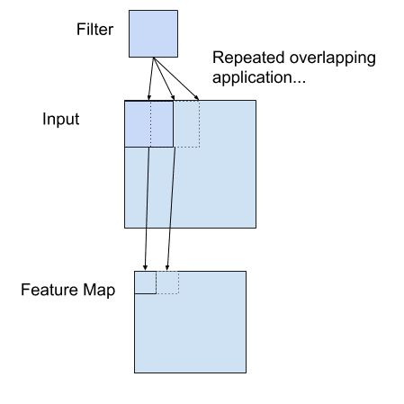
A convolution is the simple application of a filter to an input that results in an activation. Repeated application of the same filter to an input results in a map of activations called a feature map, indicating the locations and strength of a detected feature in an input, such as an image.
The innovation of convolutional neural networks is the ability to automatically learn a large number of filters in parallel specific to a training dataset under the constraints of a specific predictive modeling problem, such as image classification. The result is highly specific features that can be detected anywhere on input images.
In this tutorial, you will discover how convolutions work in the convolutional neural network.
After completing this tutorial, you will know:
Convolutional neural networks apply a filter to an input to create a feature map that summarizes the presence of detected features in the input.
Filters can be handcrafted, such as line detectors, but the innovation of convolutional neural networks is to learn the filters during training in the context of a specific prediction problem.
How to calculate the feature map for one- and two-dimensional convolutional layers in a convolutional neural network.
Kick-start your project with my new book Deep Learning for Computer Vision, including step-by-step tutorials and the Python source code files for all examples.
Let’s get started.
A Gentle Introduction to Convolutional Layers for Deep Learning Neural Networks Photo by mendhak, some rights reserved.
Tutorial Overview
This tutorial is divided into four parts; they are:
Convolution in Convolutional Neural Networks
Convolution in Computer Vision
Power of Learned Filters
Worked Example of Convolutional Layers
Want Results with Deep Learning for Computer Vision?
Take my free 7-day email crash course now (with sample code).
Click to sign-up and also get a free PDF Ebook version of the course.
Convolution in Convolutional Neural Networks
The convolutional neural network, or CNN for short, is a specialized type of neural network model designed for working with two-dimensional image data, although they can be used with one-dimensional and three-dimensional data.
Central to the convolutional neural network is the convolutional layer that gives the network its name. This layer performs an operation called a “convolution“.
In the context of a convolutional neural network, a convolution is a linear operation that involves the multiplication of a set of weights with the input, much like a traditional neural network. Given that the technique was designed for two-dimensional input, the multiplication is performed between an array of input data and a two-dimensional array of weights, called a filter or a kernel.
The filter is smaller than the input data and the type of multiplication applied between a filter-sized patch of the input and the filter is a dot product. A dot product is the element-wise multiplication between the filter-sized patch of the input and filter, which is then summed, always resulting in a single value. Because it results in a single value, the operation is often referred to as the “scalar product“.
Using a filter smaller than the input is intentional as it allows the same filter (set of weights) to be multiplied by the input array multiple times at different points on the input. Specifically, the filter is applied systematically to each overlapping part or filter-sized patch of the input data, left to right, top to bottom.
This systematic application of the same filter across an image is a powerful idea. If the filter is designed to detect a specific type of feature in the input, then the application of that filter systematically across the entire input image allows the filter an opportunity to discover that feature anywhere in the image. This capability is commonly referred to as translation invariance, e.g. the general interest in whether the feature is present rather than where it was present.
Invariance to local translation can be a very useful property if we care more about whether some feature is present than exactly where it is. For example, when determining whether an image contains a face, we need not know the location of the eyes with pixel-perfect accuracy, we just need to know that there is an eye on the left side of the face and an eye on the right side of the face.
The output from multiplying the filter with the input array one time is a single value. As the filter is applied multiple times to the input array, the result is a two-dimensional array of output values that represent a filtering of the input. As such, the two-dimensional output array from this operation is called a “feature map“.
Once a feature map is created, we can pass each value in the feature map through a nonlinearity, such as a ReLU, much like we do for the outputs of a fully connected layer.
Example of a Filter Applied to a Two-Dimensional Input to Create a Feature Map
If you come from a digital signal processing field or related area of mathematics, you may understand the convolution operation on a matrix as something different. Specifically, the filter (kernel) is flipped prior to being applied to the input. Technically, the convolution as described in the use of convolutional neural networks is actually a “cross-correlation”. Nevertheless, in deep learning, it is referred to as a “convolution” operation.
Many machine learning libraries implement cross-correlation but call it convolution.
In summary, we have a input, such as an image of pixel values, and we have a filter, which is a set of weights, and the filter is systematically applied to the input data to create a feature map.
Convolution in Computer Vision
The idea of applying the convolutional operation to image data is not new or unique to convolutional neural networks; it is a common technique used in computer vision.
Historically, filters were designed by hand by computer vision experts, which were then applied to an image to result in a feature map or output from applying the filter then makes the analysis of the image easier in some way.
For example, below is a hand crafted 3×3 element filter for detecting vertical lines:
1
2
3
0.0, 1.0, 0.0
0.0, 1.0, 0.0
0.0, 1.0, 0.0
Applying this filter to an image will result in a feature map that only contains vertical lines. It is a vertical line detector.
You can see this from the weight values in the filter; any pixels values in the center vertical line will be positively activated and any on either side will be negatively activated. Dragging this filter systematically across pixel values in an image can only highlight vertical line pixels.
A horizontal line detector could also be created and also applied to the image, for example:
1
2
3
0.0, 0.0, 0.0
1.0, 1.0, 1.0
0.0, 0.0, 0.0
Combining the results from both filters, e.g. combining both feature maps, will result in all of the lines in an image being highlighted.
A suite of tens or even hundreds of other small filters can be designed to detect other features in the image.
The innovation of using the convolution operation in a neural network is that the values of the filter are weights to be learned during the training of the network.
The network will learn what types of features to extract from the input. Specifically, training under stochastic gradient descent, the network is forced to learn to extract features from the image that minimize the loss for the specific task the network is being trained to solve, e.g. extract features that are the most useful for classifying images as dogs or cats.
In this context, you can see that this is a powerful idea.
Power of Learned Filters
Learning a single filter specific to a machine learning task is a powerful technique.
Yet, convolutional neural networks achieve much more in practice.
Multiple Filters
Convolutional neural networks do not learn a single filter; they, in fact, learn multiple features in parallel for a given input.
For example, it is common for a convolutional layer to learn from 32 to 512 filters in parallel for a given input.
This gives the model 32, or even 512, different ways of extracting features from an input, or many different ways of both “learning to see” and after training, many different ways of “seeing” the input data.
This diversity allows specialization, e.g. not just lines, but the specific lines seen in your specific training data.
Multiple Channels
Color images have multiple channels, typically one for each color channel, such as red, green, and blue.
From a data perspective, that means that a single image provided as input to the model is, in fact, three images.
A filter must always have the same number of channels as the input, often referred to as “depth“. If an input image has 3 channels (e.g. a depth of 3), then a filter applied to that image must also have 3 channels (e.g. a depth of 3). In this case, a 3×3 filter would in fact be 3x3x3 or [3, 3, 3] for rows, columns, and depth. Regardless of the depth of the input and depth of the filter, the filter is applied to the input using a dot product operation which results in a single value.
This means that if a convolutional layer has 32 filters, these 32 filters are not just two-dimensional for the two-dimensional image input, but are also three-dimensional, having specific filter weights for each of the three channels. Yet, each filter results in a single feature map. Which means that the depth of the output of applying the convolutional layer with 32 filters is 32 for the 32 feature maps created.
Multiple Layers
Convolutional layers are not only applied to input data, e.g. raw pixel values, but they can also be applied to the output of other layers.
The stacking of convolutional layers allows a hierarchical decomposition of the input.
Consider that the filters that operate directly on the raw pixel values will learn to extract low-level features, such as lines.
The filters that operate on the output of the first line layers may extract features that are combinations of lower-level features, such as features that comprise multiple lines to express shapes.
This process continues until very deep layers are extracting faces, animals, houses, and so on.
This is exactly what we see in practice. The abstraction of features to high and higher orders as the depth of the network is increased.
Worked Example of Convolutional Layers
The Keras deep learning library provides a suite of convolutional layers.
We can better understand the convolution operation by looking at some worked examples with contrived data and handcrafted filters.
In this section, we’ll look at both a one-dimensional convolutional layer and a two-dimensional convolutional layer example to both make the convolution operation concrete and provide a worked example of using the Keras layers.
Example of 1D Convolutional Layer
We can define a one-dimensional input that has eight elements all with the value of 0.0, with a two element bump in the middle with the values 1.0.
1
[0, 0, 0, 1, 1, 0, 0, 0]
The input to Keras must be three dimensional for a 1D convolutional layer.
The first dimension refers to each input sample; in this case, we only have one sample. The second dimension refers to the length of each sample; in this case, the length is eight. The third dimension refers to the number of channels in each sample; in this case, we only have a single channel.
Therefore, the shape of the input array will be [1, 8, 1].
1
2
3
# define input data
data=asarray([0,0,0,1,1,0,0,0])
data=data.reshape(1,8,1)
We will define a model that expects input samples to have the shape [8, 1].
The model will have a single filter with the shape of 3, or three elements wide. Keras refers to the shape of the filter as the kernel_size.
1
2
3
# create model
model=Sequential()
model.add(Conv1D(1,3,input_shape=(8,1)))
By default, the filters in a convolutional layer are initialized with random weights. In this contrived example, we will manually specify the weights for the single filter. We will define a filter that is capable of detecting bumps, that is a high input value surrounded by low input values, as we defined in our input example.
The three element filter we will define looks as follows:
1
[0, 1, 0]
The convolutional layer also has a bias input value that also requires a weight that we will set to zero.
Therefore, we can force the weights of our one-dimensional convolutional layer to use our handcrafted filter as follows:
The weights must be specified in a three-dimensional structure, in terms of rows, columns, and channels. The filter has a single row, three columns, and one channel.
We can retrieve the weights and confirm that they were set correctly.
1
2
# confirm they were stored
print(model.get_weights())
Finally, we can apply the single filter to our input data.
We can achieve this by calling the predict() function on the model. This will return the feature map directly: that is the output of applying the filter systematically across the input sequence.
1
2
3
# apply filter to input data
yhat=model.predict(data)
print(yhat)
Tying all of this together, the complete example is listed below.
Running the example first prints the weights of the network; that is the confirmation that our handcrafted filter was set in the model as we expected.
Next, the filter is applied to the input pattern and the feature map is calculated and displayed. We can see from the values of the feature map that the bump was detected correctly.
Recall that the input is an eight element vector with the values: [0, 0, 0, 1, 1, 0, 0, 0].
First, the three-element filter [0, 1, 0] was applied to the first three inputs of the input [0, 0, 0] by calculating the dot product (“.” operator), which resulted in a single output value in the feature map of zero.
Recall that a dot product is the sum of the element-wise multiplications, or here it is (0 x 0) + (1 x 0) + (0 x 0) = 0. In NumPy, this can be implemented manually as:
1
2
from numpy import asarray
print(asarray([0,1,0]).dot(asarray([0,0,0])))
In our manual example, this is as follows:
1
[0, 1, 0] . [0, 0, 0] = 0
The filter was then moved along one element of the input sequence and the process was repeated; specifically, the same filter was applied to the input sequence at indexes 1, 2, and 3, which also resulted in a zero output in the feature map.
1
[0, 1, 0] . [0, 0, 1] = 0
We are being systematic, so again, the filter is moved along one more element of the input and applied to the input at indexes 2, 3, and 4. This time the output is a value of one in the feature map. We detected the feature and activated appropriately.
1
[0, 1, 0] . [0, 1, 1] = 1
The process is repeated until we calculate the entire feature map.
1
[0, 0, 1, 1, 0, 0]
Note that the feature map has six elements, whereas our input has eight elements. This is an artefact of how the filter was applied to the input sequence. There are other ways to apply the filter to the input sequence that changes the shape of the resulting feature map, such as padding, but we will not discuss these methods in this post.
You can imagine that with different inputs, we may detect the feature with more or less intensity, and with different weights in the filter, that we would detect different features in the input sequence.
Example of 2D Convolutional Layer
We can expand the bump detection example in the previous section to a vertical line detector in a two-dimensional image.
Again, we can constrain the input, in this case to a square 8×8 pixel input image with a single channel (e.g. grayscale) with a single vertical line in the middle.
1
2
3
4
5
6
7
8
[0, 0, 0, 1, 1, 0, 0, 0]
[0, 0, 0, 1, 1, 0, 0, 0]
[0, 0, 0, 1, 1, 0, 0, 0]
[0, 0, 0, 1, 1, 0, 0, 0]
[0, 0, 0, 1, 1, 0, 0, 0]
[0, 0, 0, 1, 1, 0, 0, 0]
[0, 0, 0, 1, 1, 0, 0, 0]
[0, 0, 0, 1, 1, 0, 0, 0]
The input to a Conv2D layer must be four-dimensional.
The first dimension defines the samples; in this case, there is only a single sample. The second dimension defines the number of rows; in this case, eight. The third dimension defines the number of columns, again eight in this case, and finally the number of channels, which is one in this case.
Therefore, the input must have the four-dimensional shape [samples, rows, columns, channels] or [1, 8, 8, 1] in this case.
1
2
3
4
5
6
7
8
9
10
11
# define input data
data=[[0,0,0,1,1,0,0,0],
[0,0,0,1,1,0,0,0],
[0,0,0,1,1,0,0,0],
[0,0,0,1,1,0,0,0],
[0,0,0,1,1,0,0,0],
[0,0,0,1,1,0,0,0],
[0,0,0,1,1,0,0,0],
[0,0,0,1,1,0,0,0]]
data=asarray(data)
data=data.reshape(1,8,8,1)
We will define the Conv2D with a single filter as we did in the previous section with the Conv1D example.
The filter will be two-dimensional and square with the shape 3×3. The layer will expect input samples to have the shape [columns, rows, channels] or [8,8,1].
1
2
3
# create model
model=Sequential()
model.add(Conv2D(1,(3,3),input_shape=(8,8,1)))
We will define a vertical line detector filter to detect the single vertical line in our input data.
The filter looks as follows:
1
2
3
0, 1, 0
0, 1, 0
0, 1, 0
We can implement this as follows:
1
2
3
4
5
6
7
8
9
# define a vertical line detector
detector=[[[[0]],[[1]],[[0]]],
[[[0]],[[1]],[[0]]],
[[[0]],[[1]],[[0]]]]
weights=[asarray(detector),asarray([0.0])]
# store the weights in the model
model.set_weights(weights)
# confirm they were stored
print(model.get_weights())
Finally, we will apply the filter to the input image, which will result in a feature map that we would expect to show the detection of the vertical line in the input image.
1
2
# apply filter to input data
yhat=model.predict(data)
The shape of the feature map output will be four-dimensional with the shape [batch, rows, columns, filters]. We will be performing a single batch and we have a single filter (one filter and one input channel), therefore the output shape is [1, ?, ?, 1]. We can pretty-print the content of the single feature map as follows:
1
2
3
forrinrange(yhat.shape[1]):
# print each column in the row
print([yhat[0,r,c,0]forcinrange(yhat.shape[2])])
Tying all of this together, the complete example is listed below.
1
2
3
4
5
6
7
8
9
10
11
12
13
14
15
16
17
18
19
20
21
22
23
24
25
26
27
28
29
30
31
32
# example of calculation 2d convolutions
from numpy import asarray
from keras.models import Sequential
from keras.layers import Conv2D
# define input data
data=[[0,0,0,1,1,0,0,0],
[0,0,0,1,1,0,0,0],
[0,0,0,1,1,0,0,0],
[0,0,0,1,1,0,0,0],
[0,0,0,1,1,0,0,0],
[0,0,0,1,1,0,0,0],
[0,0,0,1,1,0,0,0],
[0,0,0,1,1,0,0,0]]
data=asarray(data)
data=data.reshape(1,8,8,1)
# create model
model=Sequential()
model.add(Conv2D(1,(3,3),input_shape=(8,8,1)))
# define a vertical line detector
detector=[[[[0]],[[1]],[[0]]],
[[[0]],[[1]],[[0]]],
[[[0]],[[1]],[[0]]]]
weights=[asarray(detector),asarray([0.0])]
# store the weights in the model
model.set_weights(weights)
# confirm they were stored
print(model.get_weights())
# apply filter to input data
yhat=model.predict(data)
forrinrange(yhat.shape[1]):
# print each column in the row
print([yhat[0,r,c,0]forcinrange(yhat.shape[2])])
Running the example first confirms that the handcrafted filter was correctly defined in the layer weights
Next, the calculated feature map is printed. We can see from the scale of the numbers that indeed the filter has detected the single vertical line with strong activation in the middle of the feature map.
First, the filter was applied to the top left corner of the image, or an image patch of 3×3 elements. Technically, the image patch is three dimensional with a single channel, and the filter has the same dimensions. We cannot implement this in NumPy using the dot() function, instead, we must use the tensordot() function so we can appropriately sum across all dimensions, for example:
1
2
3
4
5
6
7
8
9
from numpy import asarray
from numpy import tensordot
m1=asarray([[0,1,0],
[0,1,0],
[0,1,0]])
m2=asarray([[0,0,0],
[0,0,0],
[0,0,0]])
print(tensordot(m1,m2))
This calculation results in a single output value of 0.0, e.g., the feature was not detected. This gives us the first element in the top-left corner of the feature map.
Manually, this would be as follows:
1
2
3
0, 1, 0 0, 0, 0
0, 1, 0 . 0, 0, 0 = 0
0, 1, 0 0, 0, 0
The filter is moved along one column to the left and the process is repeated. Again, the feature is not detected.
1
2
3
0, 1, 0 0, 0, 1
0, 1, 0 . 0, 0, 1 = 0
0, 1, 0 0, 0, 1
One more move to the left to the next column and the feature is detected for the first time, resulting in a strong activation.
1
2
3
0, 1, 0 0, 1, 1
0, 1, 0 . 0, 1, 1 = 3
0, 1, 0 0, 1, 1
This process is repeated until the edge of the filter rests against the edge or final column of the input image. This gives the last element in the first full row of the feature map.
1
[0.0, 0.0, 3.0, 3.0, 0.0, 0.0]
The filter then moves down one row and back to the first column and the process is related from left to right to give the second row of the feature map. And on until the bottom of the filter rests on the bottom or last row of the input image.
Again, as with the previous section, we can see that the feature map is a 6×6 matrix, smaller than the 8×8 input image because of the limitations of how the filter can be applied to the input image.
Further Reading
This section provides more resources on the topic if you are looking to go deeper.
In this tutorial, you discovered how convolutions work in the convolutional neural network.
Specifically, you learned:
Convolutional neural networks apply a filter to an input to create a feature map that summarizes the presence of detected features in the input.
Filters can be handcrafted, such as line detectors, but the innovation of convolutional neural networks is to learn the filters during training in the context of a specific prediction problem.
How to calculate the feature map for one- and two-dimensional convolutional layers in a convolutional neural network.
Do you have any questions?
Ask your questions in the comments below and I will do my best to answer.
It provides self-study tutorials on topics like: classification, object detection (yolo and rcnn), face recognition (vggface and facenet), data preparation and much more...
Finally Bring Deep Learning to your Vision Projects
THANK you very much for your excellent explanations, I have two questions :
first one about how to fine tuning filters in convolution in order to extract specific feature from input images I mean can we change the filter values and how?.
second question why 32 to 512 filters? and are the values of these filters assumed by the model in stochastic way?
Same Question, I wanted to ask.
How can we choose filter’s weight if we can not then, do we take random values?
these filter weights can be learned during the training process? How?
My query is
Why do the parameters in pooling and flatten equal to zero? Is it only because while pooling -maxpooling or average pooling, the number of nodes are reduced.
And for flatten as it is converted to a single dimension array.
Thanks Jason for great article!
Could you clarify a couple of things for me?
First, is number of filters equals to number of feature maps?
It makes sense to me that layers closer to the input layer detect features like lines and shapes, and layers closer to the output detect more concret objects like desk and chairs.
However, don’t we need more number of filters to detect many small shapes and lines in the beginning of the network close to the input, and narrow them down as it gets closer to the output?
Also I would like to think that it’s better to start with smaller window (kernel) size close to the input and makes it bigger toward the output.
This makes sense in my head, but obviously this is not correct.
In models I’ve seen so far, number of filters increases, and the window size seems to stays static.
Would you mind explaining how it works?
First, thanks a million for some wonderful articles, very well presented!
I wondered, if you stack convolutional layers, each with > 1 filter, it seems the number of dimensions would be increasing. E.g. for a 2D image, first conv layer produces a 2D x number of filters, ie 3D. This becomes the input to second layer, which in turn produces 3D x number of filters of second conv layer, ie 4D.
From searching around*, I understand one may avoid this by making the third dimension in second layer equal to number of filters of first layer. Thus the second layer still produces only 3 dimensions.
Can you comment on this approach? If incorrect or subtleties are overlooked, maybe it’s worth adding a section on sequential convolutional layers to the article.
The size of the filter will shrink the input area. “same” padding can be used to avoid this.
The number of filters defines the channel or third dimension output. This does not linearly increase as one filter apply down through all channels in the input. Therefore at each layer you can choose the output depth/channels as the number of filters.
First of all, thanks a lot for all the tutorials. Well presented tutorials about basic and essential information saved me many times. I’ve been using CNN for a while and as far as I search and study, one question still remained without an answer. Based on my understanding each conv layer extracts specific types of features. Let’s say the first layer extracts all sorts of edge features (i.e horizontal, vertical, diagonal, etc.), As a result, the output of the layer are many images each showing some sort of edges. The second layer is supposed to extract texture features. Since the output of the first layer is not the original image anymore, how does the second layer extract textures out of it? Maybe my question is absurd or I did not understand the aim of convolution operation correctly. Yet, I appreciate if you correct me. Once again, thanks a lot for your tutorials and demonstrated codes.
Hi, thanks for your great article. The following paragraphs in the article puzzled me. Would you be so kind to shed light?
Extracted from the article:
“The first dimension defines the samples; in this case, there is only a single sample. The second dimension defines the number of rows; in this case, eight. The third dimension defines the number of columns, again eight in this case, and finally the number of channels, which is one in this case.
Therefore, the input must have the four-dimensional shape [samples, columns, rows, channels] or [1, 8, 8, 1] in this case.”
Is it [samples, rows, columns, channels] rather than [samples, columns, rows, channels] ?
Hi,
I am presently working on CNN for recognizing hand written characters belonging to a specific language using matlab.
After training the CNN , I am getting an validation set accuracy of about 90% but during the testing phase , I am not getting satisfactory results (the characters are getting classified wrongly).
How to get satisfactory results in both training and testing phases?
Will you pls help me regarding this issue.
Thanks in advance!
Hello Jason, you’re website has been very helpful to me, thanks a lot!
I found an error here, in the beginning you write about translation invariance when referring
to the convolution filter being applied over the whole image. But you’re quoting Goodfellow et. al. (p. 342) when they’re talking about the Pooling Operation, not the Filter sliding over the whole image.
It should be **equivariance** to translation (p. 338) when we talk about the Filter sliding over
the image finding any features new position after a picture might be translation transformed.
Where translation invariance talks about the result of pooling being *exactly the same*, when the picture is translated by 1-2 Pixel (Because Pooling will return the same value).
Invariance: same result regardless of operation applied to prior: f(g(x)) = f(x)
equivariance: result changes accordingly to operation, i.e. the feature map output changes
when a feature appears somewhere else in the picture after translation.
p. 338: f(g(x)) = g(f(x))
Hi Jason. Thank you for the article. It is really insightful.
I have a doubt that is related to using two convolution layers stacked together versus a single convolution layer.
(a) For example, how is two convolution layers that are stacked together with say 8 filters for each layer, different from a single convolution layer with 8 filters? Is stacking two convolution layers help in identifying detailed features?
(b) For the case of two convolution layers stacked together, using different filters for each layer, like 8 for first and 16 for second, gives a better or worse learning that using same filters for both the layers?
Hi, in the conv2D section, the article states “The filter is moved along one column to the left and the process is repeated. Again, the feature is not detected.” But it looks as if the filter is moving to the right, since the 1’s from the data are shifted in from the right.
Hey Jason I’ve been trying to find an article about the a 2d convolution but applied to an RGB image. In grayscale I understand, since it’s just 1 channel. But when we have three channels the filter also has a depth of 3. I assume that the red layer matches up with a single layer of the filter and does a convolution much like the grayscale. However, aren’t we left then we a feature map that has a depth of 3? One layer for each filter? I don’t understand how the feature map comes out to a depth of 1 because it’s one filter.
I understand that with multiple filters it is stacked, but how does one filter equate to one layer of depth?
I am an older engineer that came out of the image processing industry, where we had to build our own convolution engines out of discrete multipliers and accumulators (we also built our own graphics cards and you were really “hot” if your PC ran at 6 MHz). Kernel filters for image processing were fixed as per application requirements.
My understanding of DNNs using CNNs is that the kernel filters are adjusted during the training process. I could be wrong but I’m not sure if the terminology for the kernel filters is now “weights”. These “weights” are adjusted until a desired output of the DNN is reached.
I realize that there are many sets of weights representing the different convolutional filters that are used in the CNN stage. I also realize that to save space in memory this large number of weights is formatted.
My expectation is that each kernel filter would have to have its own unique space in system memory. My question is, is there a way to access the fully trained weights that act as the convolution filter? Yes, this would depend upon the formatting and the CNN framework that is used. I have done projects using the Darknet Framework and YOLO and I am currently learning Pytorch, but my question seems to be too basic.
Please correct any incorrect assumptions that I may have made.
Thank you so much for your reply. Yes, of course, you are correct about the possible number of filters being in the hundreds or thousands.
Just one more question, that I hope is not too naive. Would it be true to say that there is a direct correlation, in terms of the number of filters in a CNN based DNN, and the work that the network is required to do? For example, if the network was trained to distinguish between 100 different object types as opposed to a single object type, would there be many more filters required? Accuracy being equal for that object type.
hi Jason,
can you please explain to me how the value of the filter gets decided? is CNN randomly taking it and then after weight updation its value get updated , and can we take design its value as per our requirement? please reply
Sir
Why is the filter in convolution layer called a learnable filter.
The kernel initial values are random and it extracts the features. Where is the learning taking place. where is the updating of filter value taking place.
Hi sir, Thanks for the great tutorial.
I have two questions please.
-How the feature maps are connected in two different convolutional layers. Say we have first conv layer with 10 filters, and second conv layer with 64 filtres. The second layer is used directly after the first layer. So we have 10 feature maps as the output of the first conv layer that are passed to the next layer which is supposed to produce 64 feature maps. I wonder what is the relation between the 10 feature maps (the input of the second layer) and the 64 feature maps(the output of the same layer)?
-What is the effect of using Dropout between conv layers? does it drop feature maps? I use it in my project and it seems to perform well, but I don’t understand why.
The output of one convolutional layer will be a number of feature maps. These are matrices of numbers or “images” that can be fed into the next set of convolutional layers directly – just like we fed an image into the first convolutional layer.
Typically we have pooling layers sitting between convolutional layers to make the matrices (images) smaller on the way through.
Great. Thanks for your answer.
I still don’t understand how the dropout works in between convolutional layers. I know that it drops neurons in dense layers, but since we have feature maps that are passed between conv layers, I don’t really get how it operates on those feature maps. Could you please clarify it for me? or recommend some useful resources?
You have got an excellent understanding of what the readers would want and where should some extra emphasis be applied, so as the readers could understand better. I mean its in every way apt to understand the mentioned concept and get intuitions. Thanks a lot for this great work.
thank you Jason, you always have my back.
I have one question after max poling the matrix flattened to enter neural nets so how backpropagation happens in CNN like how kernels updated.
Hi Jason. You gave an excellent explanation of CNN. Thanks a lot! I have a small question. How should we decide the shape of the filter and also number of filters needed?
First of all, thank you so much for all the great content! I really like your explanations and have learned so much just from reading your posts!
I had a question regarding filters. You mention that a convolutional layer will use many filters (e.g. 32, 64, 128) but I don’t really understand how those filters would differ. Could you explain how the filters would learn different features, despite being applied to the same image?
Assume you have an image of fairly large size. One feature you may want to find is the bright spots on the image. You can use a 32×32 filter and average pooling to find the average brightness in any 32×32 region, or a 128×128 filter in 128×128 region. Hence the filter size will give you a different field of view.
Thanks for your reply! Your answer sounds like we are applying a single feature to the image, whether it is 3×3 or 32×32, etc. However, I was under the impression that a layer like:
would create many filters (32 in this case). Is that true? And if it is, my question is more around how these features are different from each other even though they are applied to the same image.
Haven’t seen this stated explicitly anywhere and was hoping you might be able to provide clarity. Say I have a bunch of 64,64,3 images but instead of having them stacked like :,64,64,3, I have them organized into higher dimensions for modeling purposes, for instance, (:,5,5,5,64,64,3). Then I run a 2D convolution (tensorflow) with stride=1 and get (:,5,5,5,64,64,1). Can I assume that the convolution iterated over all 5x5x5=125 instances of 64x64x3 images per batch sample; thus intuitively maintaining the integrity of my structure? My hope is that it just defaults to the three highest dimensions and is smart enough to iterate over all others.
Python is a bit opaque to me, so I’m a little nervous about making assumptions.
Thanks for the link. I’m pretty functional in Python, though. I’m just used to being able to see the underlying data structures at the address and bit level in C++/C when I want to understand how a library is working. 😉
More interested in the assumptions that TensorFlow is making under the hood (or at least not clearly documented). Guess I can just Reshape( ) the lower dims but was wondering if was unnecessary.
Hi Jason,
In a standard U-net there is an input layer, followed by 2 layers which utilise 64 kernels, obviously there are 64 kernels in the first layer and so 64 feature maps are produced, this seems intuitive to me. However in the second layer, you have 64 feature maps and 64 kernels, I would thus expect the number of feature maps in the subsequent layer to be 64^2 feature maps – however clearly there are only 64 based on the architectural diagram. Does this happen because the feature maps are aggregated before they pass through the second layer. If this is not the case please can you give me an explanation
Are you sure, I have read elsewhere that each subsequent feature map is only considered by one kernel in subsequent layers, i.e. the feature maps 1-64 pass through another cnn layer, the number of kernels defined are 64, and each of the kernels acts upon only one of the feature maps. So you would have kern1 acting upon fmap1 and kern2 acting on fmap2 …. kern 64 acting on fmap64. But you would never have kern64 acting on fmap22. Could you please clarifythis
Are you sure, I have read elsewhere that each subsequent feature map is only considered by one kernel in subsequent layers, i.e. the feature maps 1-64 pass through another cnn layer, the number of kernels defined are 64, and each of the kernels acts upon only one of the feature maps. So you would have kern1 acting upon fmap1 and kern2 acting on fmap2 …. kern 64 acting on fmap64. But you would never have kern64 acting on fmap22. Could you please clarifythisAre you sure, I have read elsewhere that each subsequent feature map is only considered by one kernel in subsequent layers, i.e. the feature maps 1-64 pass through another cnn layer, the number of kernels defined are 64, and each of the kernels acts upon only one of the feature maps. So you would have kern1 acting upon fmap1 and kern2 acting on fmap2 …. kern 64 acting on fmap64. But you would never have kern64 acting on fmap22. Could you please clarify this


")
THANK you very much for your excellent explanations, I have two questions :
first one about how to fine tuning filters in convolution in order to extract specific feature from input images I mean can we change the filter values and how?.
second question why 32 to 512 filters? and are the values of these filters assumed by the model in stochastic way?
Thanks. Great questions!
No, the filter values (weights) are learned. They are typically not manually modified/specified.
The number of filters is a hyperparameter that is best set via trial and error:
https://machinelearningmastery.com/how-to-configure-the-number-of-layers-and-nodes-in-a-neural-network/
Same Question, I wanted to ask.
How can we choose filter’s weight if we can not then, do we take random values?
these filter weights can be learned during the training process? How?
Hi Isha…The following resource may add clarity:
https://machinelearningmastery.com/why-initialize-a-neural-network-with-random-weights/
I am still confused that how the weights are tuned in convolutional layer
Hi Harsh…The following resource may be of interest:
https://datascience.stackexchange.com/questions/25754/updating-the-weights-of-the-filters-in-a-cnn
Good Explanation!
My query is
Why do the parameters in pooling and flatten equal to zero? Is it only because while pooling -maxpooling or average pooling, the number of nodes are reduced.
And for flatten as it is converted to a single dimension array.
Great question!
Those layers have no weights, they just transform the shape of the input in the case of flatten, or select a subset of values in the case of poling.
Thanks Jason
Thanks Jason for great article!
Could you clarify a couple of things for me?
First, is number of filters equals to number of feature maps?
It makes sense to me that layers closer to the input layer detect features like lines and shapes, and layers closer to the output detect more concret objects like desk and chairs.
However, don’t we need more number of filters to detect many small shapes and lines in the beginning of the network close to the input, and narrow them down as it gets closer to the output?
Also I would like to think that it’s better to start with smaller window (kernel) size close to the input and makes it bigger toward the output.
This makes sense in my head, but obviously this is not correct.
In models I’ve seen so far, number of filters increases, and the window size seems to stays static.
Would you mind explaining how it works?
Yes, the number of filters == the number of feature maps, in general.
Intuitions between the number fo filters and filter sizes and what they are detecting seem to breakdown. Model architectures are empirical, not based on theory, for example:
https://machinelearningmastery.com/review-of-architectural-innovations-for-convolutional-neural-networks-for-image-classification/
First, thanks a million for some wonderful articles, very well presented!
I wondered, if you stack convolutional layers, each with > 1 filter, it seems the number of dimensions would be increasing. E.g. for a 2D image, first conv layer produces a 2D x number of filters, ie 3D. This becomes the input to second layer, which in turn produces 3D x number of filters of second conv layer, ie 4D.
From searching around*, I understand one may avoid this by making the third dimension in second layer equal to number of filters of first layer. Thus the second layer still produces only 3 dimensions.
Can you comment on this approach? If incorrect or subtleties are overlooked, maybe it’s worth adding a section on sequential convolutional layers to the article.
* https://datascience.stackexchange.com/questions/9175/how-do-subsequent-convolution-layers-work?newreg=82cdb799f5f04512a8c00e2a7b445c95
Thanks again!
Good question.
The size of the filter will shrink the input area. “same” padding can be used to avoid this.
The number of filters defines the channel or third dimension output. This does not linearly increase as one filter apply down through all channels in the input. Therefore at each layer you can choose the output depth/channels as the number of filters.
Does that help?
First of all, thanks a lot for all the tutorials. Well presented tutorials about basic and essential information saved me many times. I’ve been using CNN for a while and as far as I search and study, one question still remained without an answer. Based on my understanding each conv layer extracts specific types of features. Let’s say the first layer extracts all sorts of edge features (i.e horizontal, vertical, diagonal, etc.), As a result, the output of the layer are many images each showing some sort of edges. The second layer is supposed to extract texture features. Since the output of the first layer is not the original image anymore, how does the second layer extract textures out of it? Maybe my question is absurd or I did not understand the aim of convolution operation correctly. Yet, I appreciate if you correct me. Once again, thanks a lot for your tutorials and demonstrated codes.
Yes, the layers close to input extract simple features and the layers closer to output extract higher order features.
Each filter is different, so we are extracting 128 or 256 different features at a given layer.
This might help to give you an example of what is being extracted:
https://machinelearningmastery.com/how-to-visualize-filters-and-feature-maps-in-convolutional-neural-networks/
Hi, thanks for your great article. The following paragraphs in the article puzzled me. Would you be so kind to shed light?
Extracted from the article:
“The first dimension defines the samples; in this case, there is only a single sample. The second dimension defines the number of rows; in this case, eight. The third dimension defines the number of columns, again eight in this case, and finally the number of channels, which is one in this case.
Therefore, the input must have the four-dimensional shape [samples, columns, rows, channels] or [1, 8, 8, 1] in this case.”
Is it [samples, rows, columns, channels] rather than [samples, columns, rows, channels] ?
Looks like a typo, fixed. Thanks!
Oh, thank you. I never crossed that tutorial page. It is really helpful.
No problem.
I intend to know about various lightweight cnn( deep learning Networks) and references
How lightweight cnn are different from series and DAG cnn Networks
Are shufflenet, mobilenetv2 and squeezenet models are lightweight
What do you mean by “lightweight cnn”?
Hi,
I am presently working on CNN for recognizing hand written characters belonging to a specific language using matlab.
After training the CNN , I am getting an validation set accuracy of about 90% but during the testing phase , I am not getting satisfactory results (the characters are getting classified wrongly).
How to get satisfactory results in both training and testing phases?
Will you pls help me regarding this issue.
Thanks in advance!
That is a large topic, you can get started here:
https://machinelearningmastery.com/start-here/#better
hi can you help me?
I master student in computer science and I wont your email
You can contact me any time here:
https://machinelearningmastery.com/contact/
Sir, How can I use conv2D layers as my classification output layer for 10 class classification instead of the dense layer?
Thanks in advance!
Add a global pooling layer.
Great Tutorial
Thanks!
Hello Jason, you’re website has been very helpful to me, thanks a lot!
I found an error here, in the beginning you write about translation invariance when referring
to the convolution filter being applied over the whole image. But you’re quoting Goodfellow et. al. (p. 342) when they’re talking about the Pooling Operation, not the Filter sliding over the whole image.
It should be **equivariance** to translation (p. 338) when we talk about the Filter sliding over
the image finding any features new position after a picture might be translation transformed.
Where translation invariance talks about the result of pooling being *exactly the same*, when the picture is translated by 1-2 Pixel (Because Pooling will return the same value).
Invariance: same result regardless of operation applied to prior: f(g(x)) = f(x)
equivariance: result changes accordingly to operation, i.e. the feature map output changes
when a feature appears somewhere else in the picture after translation.
p. 338: f(g(x)) = g(f(x))
Thanks, I’m happy to hear that.
Thanks!
Hi Jason. Thank you for the article. It is really insightful.
I have a doubt that is related to using two convolution layers stacked together versus a single convolution layer.
(a) For example, how is two convolution layers that are stacked together with say 8 filters for each layer, different from a single convolution layer with 8 filters? Is stacking two convolution layers help in identifying detailed features?
(b) For the case of two convolution layers stacked together, using different filters for each layer, like 8 for first and 16 for second, gives a better or worse learning that using same filters for both the layers?
Thanks in advance!
The next layer operates on the feature maps output by the first layer.
It can help on some problems.
Hi, in the conv2D section, the article states “The filter is moved along one column to the left and the process is repeated. Again, the feature is not detected.” But it looks as if the filter is moving to the right, since the 1’s from the data are shifted in from the right.
Hey Jason I’ve been trying to find an article about the a 2d convolution but applied to an RGB image. In grayscale I understand, since it’s just 1 channel. But when we have three channels the filter also has a depth of 3. I assume that the red layer matches up with a single layer of the filter and does a convolution much like the grayscale. However, aren’t we left then we a feature map that has a depth of 3? One layer for each filter? I don’t understand how the feature map comes out to a depth of 1 because it’s one filter.
I understand that with multiple filters it is stacked, but how does one filter equate to one layer of depth?
Yes. One feature map per filter and channel.
This may help:
https://machinelearningmastery.com/how-to-develop-a-cnn-from-scratch-for-cifar-10-photo-classification/
Maybe this will help:
https://machinelearningmastery.com/a-gentle-introduction-to-channels-first-and-channels-last-image-formats-for-deep-learning/
what happen if we decrease filter size In Cnn like 64,32,16 filters, instead of increasing filter size?
It will change the capability and in turn the performance of the model. Try it and see.
I am an older engineer that came out of the image processing industry, where we had to build our own convolution engines out of discrete multipliers and accumulators (we also built our own graphics cards and you were really “hot” if your PC ran at 6 MHz). Kernel filters for image processing were fixed as per application requirements.
My understanding of DNNs using CNNs is that the kernel filters are adjusted during the training process. I could be wrong but I’m not sure if the terminology for the kernel filters is now “weights”. These “weights” are adjusted until a desired output of the DNN is reached.
I realize that there are many sets of weights representing the different convolutional filters that are used in the CNN stage. I also realize that to save space in memory this large number of weights is formatted.
My expectation is that each kernel filter would have to have its own unique space in system memory. My question is, is there a way to access the fully trained weights that act as the convolution filter? Yes, this would depend upon the formatting and the CNN framework that is used. I have done projects using the Darknet Framework and YOLO and I am currently learning Pytorch, but my question seems to be too basic.
Please correct any incorrect assumptions that I may have made.
Tom
Yes, most APIs provide a way to extract the trained weights of the model. In keras it is model.get_weights() not sure about pytorch off the cuff.
You won’t have one filter, you will have hundreds or thousands depending on the depth and complexity of the model.
Thank you so much for your reply. Yes, of course, you are correct about the possible number of filters being in the hundreds or thousands.
Just one more question, that I hope is not too naive. Would it be true to say that there is a direct correlation, in terms of the number of filters in a CNN based DNN, and the work that the network is required to do? For example, if the network was trained to distinguish between 100 different object types as opposed to a single object type, would there be many more filters required? Accuracy being equal for that object type.
Thank You for your content.
Tom
Yes, we call it the capacity of the model. It’s related (a complex relationship to be sure) to the difficulty of the modeling/prediction task.
This might be relevant:
https://machinelearningmastery.com/how-to-control-neural-network-model-capacity-with-nodes-and-layers/
Hi Jason,
what will be the appropriate number of filters using 3 x 3 filter in conv layer for 224 x 224 x 3 input image?
There is no best number, try different values and discover what works well/best for your specific model and dataset.
hi Jason,
can you please explain to me how the value of the filter gets decided? is CNN randomly taking it and then after weight updation its value get updated , and can we take design its value as per our requirement? please reply
The number of layers and number of filters can be chosen a number of ways, see this:
https://machinelearningmastery.com/faq/single-faq/how-many-layers-and-nodes-do-i-need-in-my-neural-network
That made a job so much easier for me to implement;
Thanks in advance Jason;
Please continue doing the good work, your articles are so interesting and knowledgeable 😉
You’re welcome. I’m happy to hear that.
Grest work , much appreciated
Thanks!
Sir
Why is the filter in convolution layer called a learnable filter.
The kernel initial values are random and it extracts the features. Where is the learning taking place. where is the updating of filter value taking place.
I am really confused
Because the model parameters called weights are adapted based on the training data.
Hi sir, Thanks for the great tutorial.
I have two questions please.
-How the feature maps are connected in two different convolutional layers. Say we have first conv layer with 10 filters, and second conv layer with 64 filtres. The second layer is used directly after the first layer. So we have 10 feature maps as the output of the first conv layer that are passed to the next layer which is supposed to produce 64 feature maps. I wonder what is the relation between the 10 feature maps (the input of the second layer) and the 64 feature maps(the output of the same layer)?
-What is the effect of using Dropout between conv layers? does it drop feature maps? I use it in my project and it seems to perform well, but I don’t understand why.
Thanks a lot for your help.
You’re welcome.
The output of one convolutional layer will be a number of feature maps. These are matrices of numbers or “images” that can be fed into the next set of convolutional layers directly – just like we fed an image into the first convolutional layer.
Typically we have pooling layers sitting between convolutional layers to make the matrices (images) smaller on the way through.
Dropout is a type of regularization and helps us slow down learning and make the model more general (better prediction on unseen data):
https://machinelearningmastery.com/dropout-for-regularizing-deep-neural-networks/
Great. Thanks for your answer.
I still don’t understand how the dropout works in between convolutional layers. I know that it drops neurons in dense layers, but since we have feature maps that are passed between conv layers, I don’t really get how it operates on those feature maps. Could you please clarify it for me? or recommend some useful resources?
Thanks again for your help
Thanks for the tutorial!
You’re welcome!
Thank you so much – this is excellent! I love your stuff. Keep it up!
Thanks!
You have got an excellent understanding of what the readers would want and where should some extra emphasis be applied, so as the readers could understand better. I mean its in every way apt to understand the mentioned concept and get intuitions. Thanks a lot for this great work.
Thanks!
thank you Jason, you always have my back.
I have one question after max poling the matrix flattened to enter neural nets so how backpropagation happens in CNN like how kernels updated.
Good question and a great suggestion for a future blog post tutorial! Thanks.
Hi Jason. You gave an excellent explanation of CNN. Thanks a lot! I have a small question. How should we decide the shape of the filter and also number of filters needed?
You’re welcome.
You can use trial and error to determine the shape and number of filters. Or copy values used in another model as a starting point.
As usual, excellent article. Thank you for taking the time to share your knowledge!
Thanks!
An amazing article . thanks.
Thanks.
Hey Jason,
First of all, thank you so much for all the great content! I really like your explanations and have learned so much just from reading your posts!
I had a question regarding filters. You mention that a convolutional layer will use many filters (e.g. 32, 64, 128) but I don’t really understand how those filters would differ. Could you explain how the filters would learn different features, despite being applied to the same image?
Thanks!
Assume you have an image of fairly large size. One feature you may want to find is the bright spots on the image. You can use a 32×32 filter and average pooling to find the average brightness in any 32×32 region, or a 128×128 filter in 128×128 region. Hence the filter size will give you a different field of view.
Hey Jason,
Thanks for your reply! Your answer sounds like we are applying a single feature to the image, whether it is 3×3 or 32×32, etc. However, I was under the impression that a layer like:
model.add(Conv2D(32, (3, 3), activation=’relu’, kernel_initializer=’he_uniform’, padding=’same’, input_shape=(200, 200, 3)))
would create many filters (32 in this case). Is that true? And if it is, my question is more around how these features are different from each other even though they are applied to the same image.
Thanks again! Really appreciate all the content!
*how these filters are different from each other
Your understand is correct. For how different filters are different from each other, I don’t know. But when you train the network, probably it will magically converge to something different (e.g., one pick up the horizontal edge, and the other pick up vertical edge). May be you would like to read this post: https://machinelearningmastery.com/how-to-visualize-filters-and-feature-maps-in-convolutional-neural-networks/
That was very interesting. Thank you!
Haven’t seen this stated explicitly anywhere and was hoping you might be able to provide clarity. Say I have a bunch of 64,64,3 images but instead of having them stacked like :,64,64,3, I have them organized into higher dimensions for modeling purposes, for instance, (:,5,5,5,64,64,3). Then I run a 2D convolution (tensorflow) with stride=1 and get (:,5,5,5,64,64,1). Can I assume that the convolution iterated over all 5x5x5=125 instances of 64x64x3 images per batch sample; thus intuitively maintaining the integrity of my structure? My hope is that it just defaults to the three highest dimensions and is smart enough to iterate over all others.
Python is a bit opaque to me, so I’m a little nervous about making assumptions.
Hi diospyros…You may find the following resource of interest to build Python skills.
https://machinelearningmastery.com/start-here/#pythonskills
Thanks for the link. I’m pretty functional in Python, though. I’m just used to being able to see the underlying data structures at the address and bit level in C++/C when I want to understand how a library is working. 😉
More interested in the assumptions that TensorFlow is making under the hood (or at least not clearly documented). Guess I can just Reshape( ) the lower dims but was wondering if was unnecessary.
perfect explenation
Thank you for your feedback! We appreciate it!
Hi Jason,
In a standard U-net there is an input layer, followed by 2 layers which utilise 64 kernels, obviously there are 64 kernels in the first layer and so 64 feature maps are produced, this seems intuitive to me. However in the second layer, you have 64 feature maps and 64 kernels, I would thus expect the number of feature maps in the subsequent layer to be 64^2 feature maps – however clearly there are only 64 based on the architectural diagram. Does this happen because the feature maps are aggregated before they pass through the second layer. If this is not the case please can you give me an explanation
Hi Adam…Your understanding is correct!
Are you sure, I have read elsewhere that each subsequent feature map is only considered by one kernel in subsequent layers, i.e. the feature maps 1-64 pass through another cnn layer, the number of kernels defined are 64, and each of the kernels acts upon only one of the feature maps. So you would have kern1 acting upon fmap1 and kern2 acting on fmap2 …. kern 64 acting on fmap64. But you would never have kern64 acting on fmap22. Could you please clarifythis
Are you sure, I have read elsewhere that each subsequent feature map is only considered by one kernel in subsequent layers, i.e. the feature maps 1-64 pass through another cnn layer, the number of kernels defined are 64, and each of the kernels acts upon only one of the feature maps. So you would have kern1 acting upon fmap1 and kern2 acting on fmap2 …. kern 64 acting on fmap64. But you would never have kern64 acting on fmap22. Could you please clarifythisAre you sure, I have read elsewhere that each subsequent feature map is only considered by one kernel in subsequent layers, i.e. the feature maps 1-64 pass through another cnn layer, the number of kernels defined are 64, and each of the kernels acts upon only one of the feature maps. So you would have kern1 acting upon fmap1 and kern2 acting on fmap2 …. kern 64 acting on fmap64. But you would never have kern64 acting on fmap22. Could you please clarify this