Convolutional Neural Network Model Innovations for Image Classification

A Gentle Introduction to the Innovations in LeNet, AlexNet, VGG, Inception, and ResNet Convolutional Neural Networks.

Convolutional neural networks are comprised of two very simple elements, namely convolutional layers and pooling layers.

Although simple, there are near-infinite ways to arrange these layers for a given computer vision problem.

Fortunately, there are both common patterns for configuring these layers and architectural innovations that you can use in order to develop very deep convolutional neural networks. Studying these architectural design decisions developed for state-of-the-art image classification tasks can provide both a rationale and intuition for how to use these designs when designing your own deep convolutional neural network models.

In this tutorial, you will discover the key architecture milestones for the use of convolutional neural networks for challenging image classification problems.

After completing this tutorial, you will know:

• How to pattern the number of filters and filter sizes when implementing convolutional neural networks.
• How to arrange convolutional and pooling layers in a uniform pattern to develop well-performing models.
• How to use the inception module and residual module to develop much deeper convolutional networks.

Kick-start your project with my new book Deep Learning for Computer Vision, including step-by-step tutorials and the Python source code files for all examples.

Let’s get started.

• Update Apr/2019: Corrected description of filter sizes for LeNet (thanks Huang).

Tutorial Overview

This tutorial is divided into six parts; they are:

1. Architectural Design for CNNs
2. LeNet-5
3. AlexNet
4. VGG
5. Inception and GoogLeNet
6. Residual Network or ResNet

Architectural Design for CNNs

The elements of a convolutional neural network, such as convolutional and pooling layers, are relatively straightforward to understand.

The challenging part of using convolutional neural networks in practice is how to design model architectures that best use these simple elements.

A useful approach to learning how to design effective convolutional neural network architectures is to study successful applications. This is particularly straightforward to do because of the intense study and application of CNNs through 2012 to 2016 for the ImageNet Large Scale Visual Recognition Challenge, or ILSVRC. This challenge resulted in both the rapid advancement in the state of the art for very difficult computer vision tasks and the development of general innovations in the architecture of convolutional neural network models.

We will begin with the LeNet-5 that is often described as the first successful and important application of CNNs prior to the ILSVRC, then look at four different winning architectural innovations for the convolutional neural network developed for the ILSVRC, namely, AlexNet, VGG, Inception, and ResNet.

By understanding these milestone models and their architecture or architectural innovations from a high-level, you will develop both an appreciation for the use of these architectural elements in modern applications of CNN in computer vision, and be able to identify and choose architecture elements that may be useful in the design of your own models.

LeNet-5

Perhaps the first widely known and successful application of convolutional neural networks was LeNet-5, described by Yann LeCun, et al. in their 1998 paper titled “Gradient-Based Learning Applied to Document Recognition” (get the PDF).

The system was developed for use in a handwritten character recognition problem and demonstrated on the MNIST standard dataset, achieving approximately 99.2% classification accuracy (or a 0.8% error rate). The network was then described as the central technique in a broader system referred to as Graph Transformer Networks.

It is a long paper, and perhaps the best part to focus on is Section II. B. that describes the LeNet-5 architecture. In the section, the paper describes the network as having seven layers with input grayscale images having the shape 32×32, the size of images in the MNIST dataset.

The model proposes a pattern of a convolutional layer followed by an average pooling layer, referred to as a subsampling layer. This pattern is repeated two and a half times before the output feature maps are flattened and fed to a number of fully connected layers for interpretation and a final prediction. A picture of the network architecture is provided in the paper and reproduced below.

Architecture of the LeNet-5 Convolutional Neural Network for Handwritten Character Recognition (taken from the 1998 paper).

The pattern of blocks of convolutional layers and pooling layers grouped together and repeated remains a common pattern in designing and using convolutional neural networks today, more than twenty years later.

Interestingly, the architecture uses a small number of filters as the first hidden layer, specifically six filters each with the size of 5×5 pixels. After pooling (called a subsampling layer), another convolutional layer has many more filters, again with a smaller size but smaller than the prior convolutional layer, specifically 16 filters with a size of 5×5 pixels, again followed by pooling. In the repetition of these two blocks of convolution and pooling layers, the trend is an increase in the number of filters.

Compared to modern applications, the number of filters is also small, but the trend of increasing the number of filters with the depth of the network also remains a common pattern in modern usage of the technique.

The flattening of the feature maps and interpretation and classification of the extracted features by fully connected layers also remains a common pattern today. In modern terminology, the final section of the architecture is often referred to as the classifier, whereas the convolutional and pooling layers earlier in the model are referred to as the feature extractor.

We can summarize the key aspects of the architecture relevant in modern models as follows:

• Fixed-sized input images.
• Group convolutional and pooling layers into blocks.
• Repetition of convolutional-pooling blocks in the architecture.
• Increase in the number of filters with the depth of the network.
• Distinct feature extraction and classifier parts of the architecture.

AlexNet

The work that perhaps could be credited with sparking renewed interest in neural networks and the beginning of the dominance of deep learning in many computer vision applications was the 2012 paper by Alex Krizhevsky, et al. titled “ImageNet Classification with Deep Convolutional Neural Networks.”

The paper describes a model later referred to as “AlexNet” designed to address the ImageNet Large Scale Visual Recognition Challenge or ILSVRC-2010 competition for classifying photographs of objects into one of 1,000 different categories.

The ILSVRC was a competition held from 2011 to 2016, designed to spur innovation in the field of computer vision. Before the development of AlexNet, the task was thought very difficult and far beyond the capability of modern computer vision methods. AlexNet successfully demonstrated the capability of the convolutional neural network model in the domain, and kindled a fire that resulted in many more improvements and innovations, many demonstrated on the same ILSVRC task in subsequent years. More broadly, the paper showed that it is possible to develop deep and effective end-to-end models for a challenging problem without using unsupervised pretraining techniques that were popular at the time.

Important in the design of AlexNet was a suite of methods that were new or successful, but not widely adopted at the time. Now, they have become requirements when using CNNs for image classification.

AlexNet made use of the rectified linear activation function, or ReLU, as the nonlinearly after each convolutional layer, instead of S-shaped functions such as the logistic or tanh that were common up until that point. Also, a softmax activation function was used in the output layer, now a staple for multi-class classification with neural networks.

The average pooling used in LeNet-5 was replaced with a max pooling method, although in this case, overlapping pooling was found to outperform non-overlapping pooling that is commonly used today (e.g. stride of pooling operation is the same size as the pooling operation, e.g. 2 by 2 pixels). To address overfitting, the newly proposed dropout method was used between the fully connected layers of the classifier part of the model to improve generalization error.

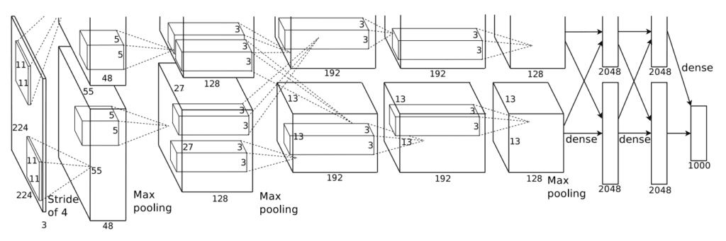
The architecture of AlexNet is deep and extends upon some of the patterns established with LeNet-5. The image below, taken from the paper, summarizes the model architecture, in this case, split into two pipelines to train on the GPU hardware of the time.

Architecture of the AlexNet Convolutional Neural Network for Object Photo Classification (taken from the 2012 paper).

The model has five convolutional layers in the feature extraction part of the model and three fully connected layers in the classifier part of the model.

Input images were fixed to the size 224×224 with three color channels. In terms of the number of filters used in each convolutional layer, the pattern of increasing the number of filters with depth seen in LeNet was mostly adhered to, in this case, the sizes: 96, 256, 384, 384, and 256. Similarly, the pattern of decreasing the size of the filter (kernel) with depth was used, starting from the smaller size of 11×11 and decreasing to 5×5, and then to 3×3 in the deeper layers. Use of small filters such as 5×5 and 3×3 is now the norm.

A pattern of a convolutional layer followed by pooling layer was used at the start and end of the feature detection part of the model. Interestingly, a pattern of convolutional layer followed immediately by a second convolutional layer was used. This pattern too has become a modern standard.

The model was trained with data augmentation, artificially increasing the size of the training dataset and giving the model more of an opportunity to learn the same features in different orientations.

We can summarize the key aspects of the architecture relevant in modern models as follows:

• Use of the ReLU activation function after convolutional layers and softmax for the output layer.
• Use of Max Pooling instead of Average Pooling.
• Use of Dropout regularization between the fully connected layers.
• Pattern of convolutional layer fed directly to another convolutional layer.
• Use of Data Augmentation.

VGG

The development of deep convolutional neural networks for computer vision tasks appeared to be a little bit of a dark art after AlexNet.

An important work that sought to standardize architecture design for deep convolutional networks and developed much deeper and better performing models in the process was the 2014 paper titled “Very Deep Convolutional Networks for Large-Scale Image Recognition” by Karen Simonyan and Andrew Zisserman.

Their architecture is generally referred to as VGG after the name of their lab, the Visual Geometry Group at Oxford. Their model was developed and demonstrated on the sameILSVRC competition, in this case, the ILSVRC-2014 version of the challenge.

The first important difference that has become a de facto standard is the use of a large number of small filters. Specifically, filters with the size 3×3 and 1×1 with the stride of one, different from the large sized filters in LeNet-5 and the smaller but still relatively large filters and large stride of four in AlexNet.

Max pooling layers are used after most, but not all, convolutional layers, learning from the example in AlexNet, yet all pooling is performed with the size 2×2 and the same stride, that too has become a de facto standard. Specifically, the VGG networks use examples of two, three, and even four convolutional layers stacked together before a max pooling layer is used. The rationale was that stacked convolutional layers with smaller filters approximate the effect of one convolutional layer with a larger sized filter, e.g. three stacked convolutional layers with 3×3 filters approximates one convolutional layer with a 7×7 filter.

Another important difference is the very large number of filters used. The number of filters increases with the depth of the model, although starts at a relatively large number of 64 and increases through 128, 256, and 512 filters at the end of the feature extraction part of the model.

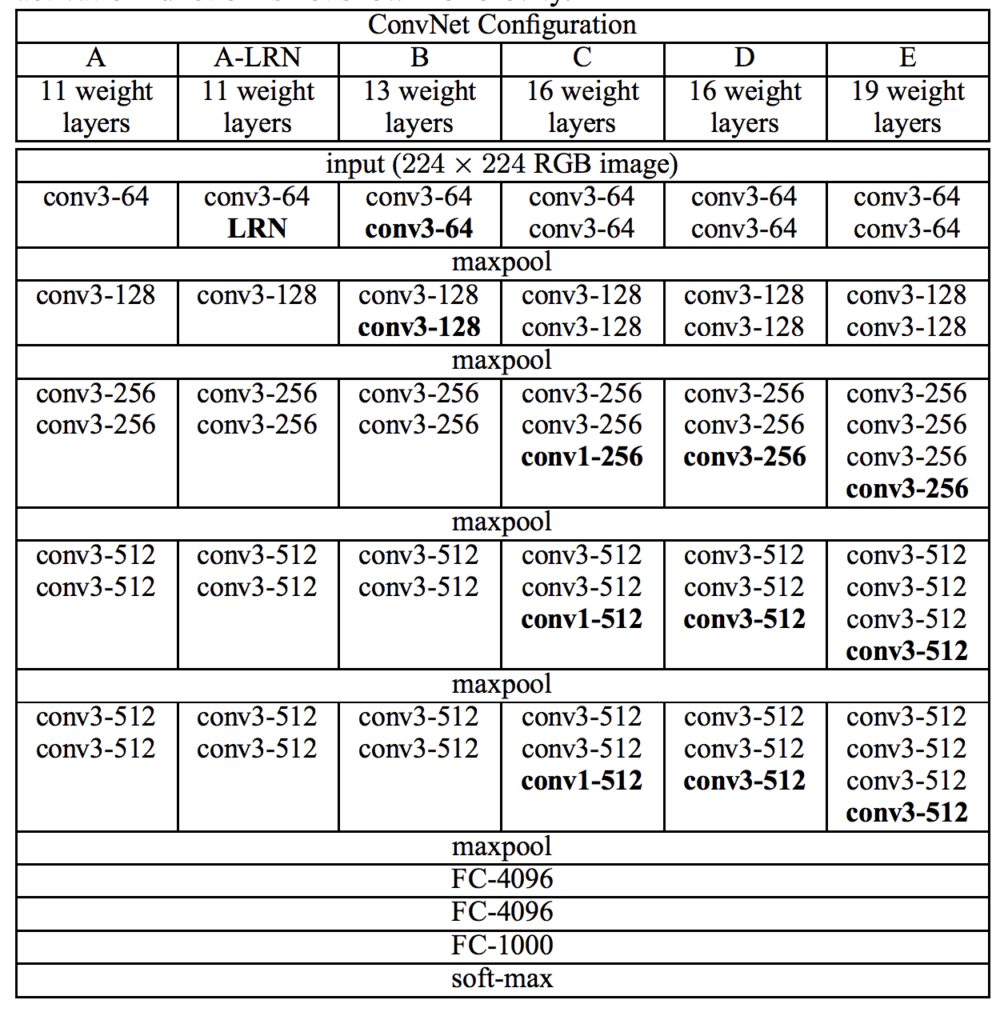
A number of variants of the architecture were developed and evaluated, although two are referred to most commonly given their performance and depth. They are named for the number of layers: they are the VGG-16 and the VGG-19 for 16 and 19 learned layers respectively.

Below is a table taken from the paper; note the two far right columns indicating the configuration (number of filters) used in the VGG-16 and VGG-19 versions of the architecture.

Architecture of the VGG Convolutional Neural Network for Object Photo Classification (taken from the 2014 paper).

The design decisions in the VGG models have become the starting point for simple and direct use of convolutional neural networks in general.

Finally, the VGG work was among the first to release the valuable model weights under a permissive license that led to a trend among deep learning computer vision researchers. This, in turn, has led to the heavy use of pre-trained models like VGG in transfer learning as a starting point on new computer vision tasks.

We can summarize the key aspects of the architecture relevant in modern models as follows:

• Use of very small convolutional filters, e.g. 3×3 and 1×1 with a stride of one.
• Use of max pooling with a size of 2×2 and a stride of the same dimensions.
• The importance of stacking convolutional layers together before using a pooling layer to define a block.
• Dramatic repetition of the convolutional-pooling block pattern.
• Development of very deep (16 and 19 layer) models.

Inception and GoogLeNet

Important innovations in the use of convolutional layers were proposed in the 2015 paper by Christian Szegedy, et al. titled “Going Deeper with Convolutions.”

In the paper, the authors propose an architecture referred to as inception (or inception v1 to differentiate it from extensions) and a specific model called GoogLeNet that achieved top results in the 2014 version of the ILSVRC challenge.

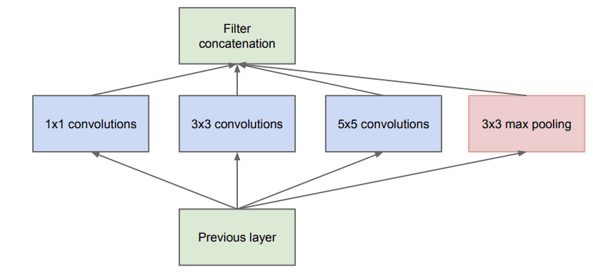
The key innovation on the inception models is called the inception module. This is a block of parallel convolutional layers with different sized filters (e.g. 1×1, 3×3, 5×5) and a 3×3 max pooling layer, the results of which are then concatenated. Below is an example of the inception module taken from the paper.

Example of the Naive Inception Module (taken from the 2015 paper).

A problem with a naive implementation of the inception model is that the number of filters (depth or channels) begins to build up fast, especially when inception modules are stacked.

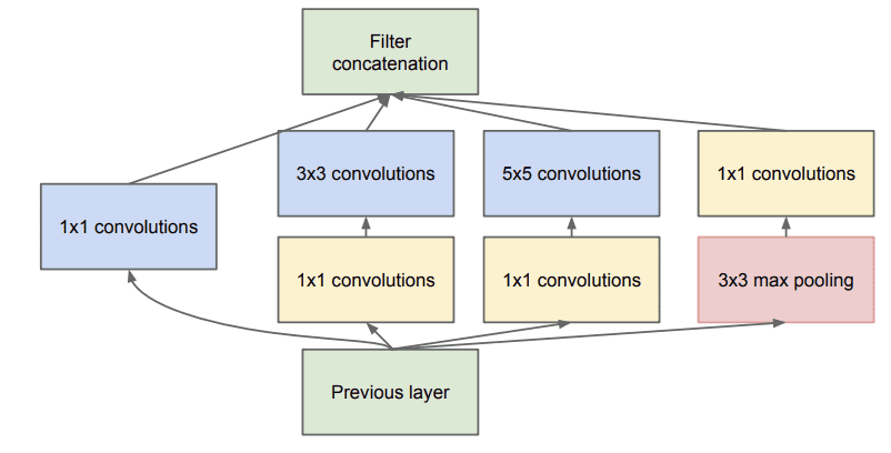
Performing convolutions with larger filter sizes (e.g. 3 and 5) can be computationally expensive on a large number of filters. To address this, 1×1 convolutional layers are used to reduce the number of filters in the inception model. Specifically before the 3×3 and 5×5 convolutional layers and after the pooling layer. The image below taken from the paper shows this change to the inception module.

Example of the Inception Module With Dimensionality Reduction (taken from the 2015 paper).

A second important design decision in the inception model was connecting the output at different points in the model. This was achieved by creating small off-shoot output networks from the main network that were trained to make a prediction. The intent was to provide an additional error signal from the classification task at different points of the deep model in order to address the vanishing gradients problem. These small output networks were then removed after training.

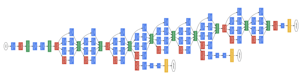
Below shows a rotated version (left-to-right for input-to-output) of the architecture of the GoogLeNet model taken from the paper using the Inception modules from the input on the left to the output classification on the right and the two additional output networks that were only used during training.

Architecture of the GoogLeNet Model Used During Training for Object Photo Classification (taken from the 2015 paper).

Interestingly, overlapping max pooling was used and a large average pooling operation was used at the end of the feature extraction part of the model prior to the classifier part of the model.

We can summarize the key aspects of the architecture relevant in modern models as follows:

• Development and repetition of the Inception module.
• Heavy use of the 1×1 convolution to reduce the number of channels.
• Use of error feedback at multiple points in the network.
• Development of very deep (22-layer) models.
• Use of global average pooling for the output of the model.

Residual Network or ResNet

A final important innovation in convolutional neural nets that we will review was proposed by Kaiming He, et al. in their 2016 paper titled “Deep Residual Learning for Image Recognition.”

In the paper, the authors proposed a very deep model called a Residual Network, or ResNet for short, an example of which achieved success on the 2015 version of the ILSVRC challenge.

Their model had an impressive 152 layers. Key to the model design is the idea of residual blocks that make use of shortcut connections. These are simply connections in the network architecture where the input is kept as-is (not weighted) and passed on to a deeper layer, e.g. skipping the next layer.

A residual block is a pattern of two convolutional layers with ReLU activation where the output of the block is combined with the input to the block, e.g. the shortcut connection. A projected version of the input used via 1×1 if the shape of the input to the block is different to the output of the block, so-called 1×1 convolutions. These are referred to as projected shortcut connections, compared to the unweighted or identity shortcut connections.

The authors start with what they call a plain network, which is a VGG-inspired deep convolutional neural network with small filters (3×3), grouped convolutional layers followed with no pooling in between, and an average pooling at the end of the feature detector part of the model prior to the fully connected output layer with a softmax activation function.

The plain network is modified to become a residual network by adding shortcut connections in order to define residual blocks. Typically the shape of the input for the shortcut connection is the same size as the output of the residual block.

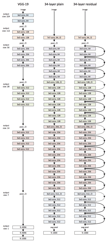
The image below was taken from the paper and from left to right compares the architecture of a VGG model, a plain convolutional model, and a version of the plain convolutional with residual modules, called a residual network.

Architecture of the Residual Network for Object Photo Classification (taken from the 2016 paper).

We can summarize the key aspects of the architecture relevant in modern models as follows:

• Use of shortcut connections.
• Development and repetition of the residual blocks.
• Development of very deep (152-layer) models.

Further Reading

This section provides more resources on the topic if you are looking to go deeper.

Papers

• Gradient-based learning applied to document recognition, (PDF) 1998.
• ImageNet Classification with Deep Convolutional Neural Networks, 2012.
• Very Deep Convolutional Networks for Large-Scale Image Recognition, 2014.
• Going Deeper with Convolutions, 2015.
• Deep Residual Learning for Image Recognition, 2016

API

• Keras Applications API

Articles

• The 9 Deep Learning Papers You Need To Know About
• A Simple Guide to the Versions of the Inception Network, 2018.
• CNN Architectures: LeNet, AlexNet, VGG, GoogLeNet, ResNet and more., 2017.

Summary

In this tutorial, you discovered the key architecture milestones for the use of convolutional neural networks for challenging image classification.

Specifically, you learned:

• How to pattern the number of filters and filter sizes when implementing convolutional neural networks.
• How to arrange convolutional and pooling layers in a uniform pattern to develop well-performing models.
• How to use the inception module and residual module to develop much deeper convolutional networks.

Do you have any questions?
Ask your questions in the comments below and I will do my best to answer.

Develop Deep Learning Models for Vision Today!

Develop Your Own Vision Models in Minutes

...with just a few lines of python code

Discover how in my new Ebook:
Deep Learning for Computer Vision

It provides self-study tutorials on topics like:
classification, object detection (yolo and rcnn), face recognition (vggface and facenet), data preparation and much more...

Finally Bring Deep Learning to your Vision Projects

Skip the Academics. Just Results.

See What's Inside