In a neural network, the activation function is responsible for transforming the summed weighted input from the node into the activation of the node or output for that input.
The rectified linear activation function or ReLU for short is a piecewise linear function that will output the input directly if it is positive, otherwise, it will output zero. It has become the default activation function for many types of neural networks because a model that uses it is easier to train and often achieves better performance.
In this tutorial, you will discover the rectified linear activation function for deep learning neural networks.
After completing this tutorial, you will know:
- The sigmoid and hyperbolic tangent activation functions cannot be used in networks with many layers due to the vanishing gradient problem.
- The rectified linear activation function overcomes the vanishing gradient problem, allowing models to learn faster and perform better.
- The rectified linear activation is the default activation when developing multilayer Perceptron and convolutional neural networks.
Kick-start your project with my new book Better Deep Learning, including step-by-step tutorials and the Python source code files for all examples.
Let’s get started.
- Jun/2019: Fixed error in the equation for He weight initialization (thanks Maltev).

A Gentle Introduction to the Rectified Linear Activation Function for Deep Learning Neural Networks
Photo by Bureau of Land Management, some rights reserved.
Tutorial Overview
This tutorial is divided into six parts; they are:
- Limitations of Sigmoid and Tanh Activation Functions
- Rectified Linear Activation Function
- How to Implement the Rectified Linear Activation Function
- Advantages of the Rectified Linear Activation
- Tips for Using the Rectified Linear Activation
- Extensions and Alternatives to ReLU
Limitations of Sigmoid and Tanh Activation Functions
A neural network is comprised of layers of nodes and learns to map examples of inputs to outputs.
For a given node, the inputs are multiplied by the weights in a node and summed together. This value is referred to as the summed activation of the node. The summed activation is then transformed via an activation function and defines the specific output or “activation” of the node.
The simplest activation function is referred to as the linear activation, where no transform is applied at all. A network comprised of only linear activation functions is very easy to train, but cannot learn complex mapping functions. Linear activation functions are still used in the output layer for networks that predict a quantity (e.g. regression problems).
Nonlinear activation functions are preferred as they allow the nodes to learn more complex structures in the data. Traditionally, two widely used nonlinear activation functions are the sigmoid and hyperbolic tangent activation functions.
The sigmoid activation function, also called the logistic function, is traditionally a very popular activation function for neural networks. The input to the function is transformed into a value between 0.0 and 1.0. Inputs that are much larger than 1.0 are transformed to the value 1.0, similarly, values much smaller than 0.0 are snapped to 0.0. The shape of the function for all possible inputs is an S-shape from zero up through 0.5 to 1.0. For a long time, through the early 1990s, it was the default activation used on neural networks.
The hyperbolic tangent function, or tanh for short, is a similar shaped nonlinear activation function that outputs values between -1.0 and 1.0. In the later 1990s and through the 2000s, the tanh function was preferred over the sigmoid activation function as models that used it were easier to train and often had better predictive performance.
… the hyperbolic tangent activation function typically performs better than the logistic sigmoid.
— Page 195, Deep Learning, 2016.
A general problem with both the sigmoid and tanh functions is that they saturate. This means that large values snap to 1.0 and small values snap to -1 or 0 for tanh and sigmoid respectively. Further, the functions are only really sensitive to changes around their mid-point of their input, such as 0.5 for sigmoid and 0.0 for tanh.
The limited sensitivity and saturation of the function happen regardless of whether the summed activation from the node provided as input contains useful information or not. Once saturated, it becomes challenging for the learning algorithm to continue to adapt the weights to improve the performance of the model.
… sigmoidal units saturate across most of their domain—they saturate to a high value when z is very positive, saturate to a low value when z is very negative, and are only strongly sensitive to their input when z is near 0.
— Page 195, Deep Learning, 2016.
Finally, as the capability of hardware increased through GPUs’ very deep neural networks using sigmoid and tanh activation functions could not easily be trained.
Layers deep in large networks using these nonlinear activation functions fail to receive useful gradient information. Error is back propagated through the network and used to update the weights. The amount of error decreases dramatically with each additional layer through which it is propagated, given the derivative of the chosen activation function. This is called the vanishing gradient problem and prevents deep (multi-layered) networks from learning effectively.
Vanishing gradients make it difficult to know which direction the parameters should move to improve the cost function
— Page 290, Deep Learning, 2016.
For an example of how ReLU can fix the vanishing gradients problem, see the tutorial:
Although the use of nonlinear activation functions allows neural networks to learn complex mapping functions, they effectively prevent the learning algorithm from working with deep networks.
Workarounds were found in the late 2000s and early 2010s using alternate network types such as Boltzmann machines and layer-wise training or unsupervised pre-training.
Want Better Results with Deep Learning?
Take my free 7-day email crash course now (with sample code).
Click to sign-up and also get a free PDF Ebook version of the course.
Rectified Linear Activation Function
In order to use stochastic gradient descent with backpropagation of errors to train deep neural networks, an activation function is needed that looks and acts like a linear function, but is, in fact, a nonlinear function allowing complex relationships in the data to be learned.
The function must also provide more sensitivity to the activation sum input and avoid easy saturation.
The solution had been bouncing around in the field for some time, although was not highlighted until papers in 2009 and 2011 shone a light on it.
The solution is to use the rectified linear activation function, or ReL for short.
A node or unit that implements this activation function is referred to as a rectified linear activation unit, or ReLU for short. Often, networks that use the rectifier function for the hidden layers are referred to as rectified networks.
Adoption of ReLU may easily be considered one of the few milestones in the deep learning revolution, e.g. the techniques that now permit the routine development of very deep neural networks.
[another] major algorithmic change that has greatly improved the performance of feedforward networks was the replacement of sigmoid hidden units with piecewise linear hidden units, such as rectified linear units.
— Page 226, Deep Learning, 2016.
The rectified linear activation function is a simple calculation that returns the value provided as input directly, or the value 0.0 if the input is 0.0 or less.
We can describe this using a simple if-statement:
|
1 2 3 4 |
if input > 0: return input else: return 0 |
We can describe this function g() mathematically using the max() function over the set of 0.0 and the input z; for example:
|
1 |
g(z) = max{0, z} |
The function is linear for values greater than zero, meaning it has a lot of the desirable properties of a linear activation function when training a neural network using backpropagation. Yet, it is a nonlinear function as negative values are always output as zero.
Because rectified linear units are nearly linear, they preserve many of the properties that make linear models easy to optimize with gradient-based methods. They also preserve many of the properties that make linear models generalize well.
— Page 175, Deep Learning, 2016.
Because the rectified function is linear for half of the input domain and nonlinear for the other half, it is referred to as a piecewise linear function or a hinge function.
However, the function remains very close to linear, in the sense that is a piecewise linear function with two linear pieces.
— Page 175, Deep Learning, 2016.
Now that we are familiar with the rectified linear activation function, let’s look at how we can implement it in Python.
How to Code the Rectified Linear Activation Function
We can implement the rectified linear activation function easily in Python.
Perhaps the simplest implementation is using the max() function; for example:
|
1 2 3 |
# rectified linear function def rectified(x): return max(0.0, x) |
We expect that any positive value will be returned unchanged whereas an input value of 0.0 or a negative value will be returned as the value 0.0.
Below are a few examples of inputs and outputs of the rectified linear activation function.
|
1 2 3 4 5 6 7 8 9 10 11 12 13 14 15 16 17 18 19 |
# demonstrate the rectified linear function # rectified linear function def rectified(x): return max(0.0, x) # demonstrate with a positive input x = 1.0 print('rectified(%.1f) is %.1f' % (x, rectified(x))) x = 1000.0 print('rectified(%.1f) is %.1f' % (x, rectified(x))) # demonstrate with a zero input x = 0.0 print('rectified(%.1f) is %.1f' % (x, rectified(x))) # demonstrate with a negative input x = -1.0 print('rectified(%.1f) is %.1f' % (x, rectified(x))) x = -1000.0 print('rectified(%.1f) is %.1f' % (x, rectified(x))) |
Running the example, we can see that positive values are returned regardless of their size, whereas negative values are snapped to the value 0.0.
|
1 2 3 4 5 |
rectified(1.0) is 1.0 rectified(1000.0) is 1000.0 rectified(0.0) is 0.0 rectified(-1.0) is 0.0 rectified(-1000.0) is 0.0 |
We can get an idea of the relationship between inputs and outputs of the function by plotting a series of inputs and the calculated outputs.
The example below generates a series of integers from -10 to 10 and calculates the rectified linear activation for each input, then plots the result.
|
1 2 3 4 5 6 7 8 9 10 11 12 13 14 |
# plot inputs and outputs from matplotlib import pyplot # rectified linear function def rectified(x): return max(0.0, x) # define a series of inputs series_in = [x for x in range(-10, 11)] # calculate outputs for our inputs series_out = [rectified(x) for x in series_in] # line plot of raw inputs to rectified outputs pyplot.plot(series_in, series_out) pyplot.show() |
Running the example creates a line plot showing that all negative values and zero inputs are snapped to 0.0, whereas the positive outputs are returned as-is, resulting in a linearly increasing slope, given that we created a linearly increasing series of positive values (e.g. 1 to 10).
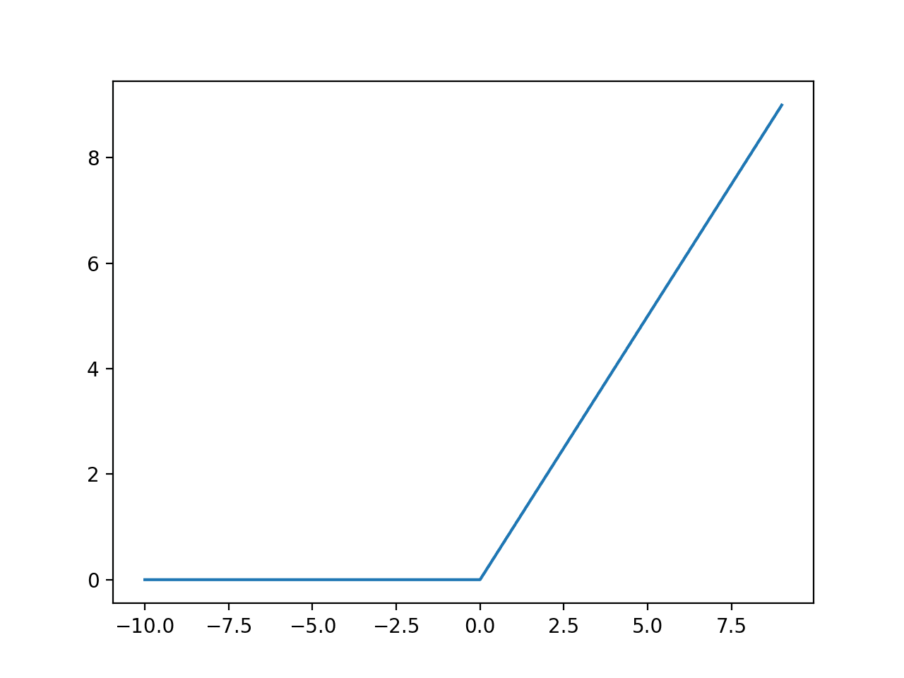
Line Plot of Rectified Linear Activation for Negative and Positive Inputs
The derivative of the rectified linear function is also easy to calculate. Recall that the derivative of the activation function is required when updating the weights of a node as part of the backpropagation of error.
The derivative of the function is the slope. The slope for negative values is 0.0 and the slope for positive values is 1.0.
Traditionally, the field of neural networks has avoided any activation function that was not completely differentiable, perhaps delaying the adoption of the rectified linear function and other piecewise-linear functions. Technically, we cannot calculate the derivative when the input is 0.0, therefore, we can assume it is zero. This is not a problem in practice.
For example, the rectified linear function g(z) = max{0, z} is not differentiable at z = 0. This may seem like it invalidates g for use with a gradient-based learning algorithm. In practice, gradient descent still performs well enough for these models to be used for machine learning tasks.
— Page 192, Deep Learning, 2016.
Using the rectified linear activation function offers many advantages; let’s take a look at a few in the next section.
Advantages of the Rectified Linear Activation Function
The rectified linear activation function has rapidly become the default activation function when developing most types of neural networks.
As such, it is important to take a moment to review some of the benefits of the approach, first highlighted by Xavier Glorot, et al. in their milestone 2012 paper on using ReLU titled “Deep Sparse Rectifier Neural Networks“.
1. Computational Simplicity.
The rectifier function is trivial to implement, requiring a max() function.
This is unlike the tanh and sigmoid activation function that require the use of an exponential calculation.
Computations are also cheaper: there is no need for computing the exponential function in activations
— Deep Sparse Rectifier Neural Networks, 2011.
2. Representational Sparsity
An important benefit of the rectifier function is that it is capable of outputting a true zero value.
This is unlike the tanh and sigmoid activation functions that learn to approximate a zero output, e.g. a value very close to zero, but not a true zero value.
This means that negative inputs can output true zero values allowing the activation of hidden layers in neural networks to contain one or more true zero values. This is called a sparse representation and is a desirable property in representational learning as it can accelerate learning and simplify the model.
An area where efficient representations such as sparsity are studied and sought is in autoencoders, where a network learns a compact representation of an input (called the code layer), such as an image or series, before it is reconstructed from the compact representation.
One way to achieve actual zeros in h for sparse (and denoising) autoencoders […] The idea is to use rectified linear units to produce the code layer. With a prior that actually pushes the representations to zero (like the absolute value penalty), one can thus indirectly control the average number of zeros in the representation.
— Page 507, Deep Learning, 2016.
3. Linear Behavior
The rectifier function mostly looks and acts like a linear activation function.
In general, a neural network is easier to optimize when its behavior is linear or close to linear.
Rectified linear units […] are based on the principle that models are easier to optimize if their behavior is closer to linear.
— Page 194, Deep Learning, 2016.
Key to this property is that networks trained with this activation function almost completely avoid the problem of vanishing gradients, as the gradients remain proportional to the node activations.
Because of this linearity, gradients flow well on the active paths of neurons (there is no gradient vanishing effect due to activation non-linearities of sigmoid or tanh units).
— Deep Sparse Rectifier Neural Networks, 2011.
4. Train Deep Networks
Importantly, the (re-)discovery and adoption of the rectified linear activation function meant that it became possible to exploit improvements in hardware and successfully train deep multi-layered networks with a nonlinear activation function using backpropagation.
In turn, cumbersome networks such as Boltzmann machines could be left behind as well as cumbersome training schemes such as layer-wise training and unlabeled pre-training.
… deep rectifier networks can reach their best performance without requiring any unsupervised pre-training on purely supervised tasks with large labeled datasets. Hence, these results can be seen as a new milestone in the attempts at understanding the difficulty in training deep but purely supervised neural networks, and closing the performance gap between neural networks learnt with and without unsupervised pre-training.
— Deep Sparse Rectifier Neural Networks, 2011.
Tips for Using the Rectified Linear Activation
In this section, we’ll take a look at some tips when using the rectified linear activation function in your own deep learning neural networks.
Use ReLU as the Default Activation Function
For a long time, the default activation to use was the sigmoid activation function. Later, it was the tanh activation function.
For modern deep learning neural networks, the default activation function is the rectified linear activation function.
Prior to the introduction of rectified linear units, most neural networks used the logistic sigmoid activation function or the hyperbolic tangent activation function.
— Page 195, Deep Learning, 2016.
Most papers that achieve state-of-the-art results will describe a network using ReLU. For example, in the milestone 2012 paper by Alex Krizhevsky, et al. titled “ImageNet Classification with Deep Convolutional Neural Networks,” the authors developed a deep convolutional neural network with ReLU activations that achieved state-of-the-art results on the ImageNet photo classification dataset.
… we refer to neurons with this nonlinearity as Rectified Linear Units (ReLUs). Deep convolutional neural networks with ReLUs train several times faster than their equivalents with tanh units.
If in doubt, start with ReLU in your neural network, then perhaps try other piecewise linear activation functions to see how their performance compares.
In modern neural networks, the default recommendation is to use the rectified linear unit or ReLU
— Page 174, Deep Learning, 2016.
Use ReLU with MLPs, CNNs, but Probably Not RNNs
The ReLU can be used with most types of neural networks.
It is recommended as the default for both Multilayer Perceptron (MLP) and Convolutional Neural Networks (CNNs).
The use of ReLU with CNNs has been investigated thoroughly, and almost universally results in an improvement in results, initially, surprisingly so.
… how do the non-linearities that follow the filter banks influence the recognition accuracy. The surprising answer is that using a rectifying non-linearity is the single most important factor in improving the performance of a recognition system.
— What is the best multi-stage architecture for object recognition?, 2009
Work investigating ReLU with CNNs is what provoked their use with other network types.
[others] have explored various rectified nonlinearities […] in the context of convolutional networks and have found them to improve discriminative performance.
— Rectified Linear Units Improve Restricted Boltzmann Machines, 2010.
When using ReLU with CNNs, they can be used as the activation function on the filter maps themselves, followed then by a pooling layer.
A typical layer of a convolutional network consists of three stages […] In the second stage, each linear activation is run through a nonlinear activation function, such as the rectified linear activation function. This stage is sometimes called the detector stage.
— Page 339, Deep Learning, 2016.
Traditionally, LSTMs use the tanh activation function for the activation of the cell state and the sigmoid activation function for the node output. Given their careful design, ReLU were thought to not be appropriate for Recurrent Neural Networks (RNNs) such as the Long Short-Term Memory Network (LSTM) by default.
At first sight, ReLUs seem inappropriate for RNNs because they can have very large outputs so they might be expected to be far more likely to explode than units that have bounded values.
— A Simple Way to Initialize Recurrent Networks of Rectified Linear Units, 2015.
Nevertheless, there has been some work on investigating the use of ReLU as the output activation in LSTMs, the result of which is a careful initialization of network weights to ensure that the network is stable prior to training. This is outlined in the 2015 paper titled “A Simple Way to Initialize Recurrent Networks of Rectified Linear Units.”
Try a Smaller Bias Input Value
The bias is the input on the node that has a fixed value.
The bias has the effect of shifting the activation function and it is traditional to set the bias input value to 1.0.
When using ReLU in your network, consider setting the bias to a small value, such as 0.1.
… it can be a good practice to set all elements of [the bias] to a small, positive value, such as 0.1. This makes it very likely that the rectified linear units will be initially active for most inputs in the training set and allow the derivatives to pass through.
— Page 193, Deep Learning, 2016.
There are some conflicting reports as to whether this is required, so compare performance to a model with a 1.0 bias input.
Use “He Weight Initialization”
Before training a neural network,the weights of the network must be initialized to small random values.
When using ReLU in your network and initializing weights to small random values centered on zero, then by default half of the units in the network will output a zero value.
For example, after uniform initialization of the weights, around 50% of hidden units continuous output values are real zeros
— Deep Sparse Rectifier Neural Networks, 2011.
There are many heuristic methods to initialize the weights for a neural network, yet there is no best weight initialization scheme and little relationship beyond general guidelines for mapping weight initialization schemes to the choice of activation function.
Prior to the wide adoption of ReLU, Xavier Glorot and Yoshua Bengio proposed an initialization scheme in their 2010 paper titled “Understanding the difficulty of training deep feedforward neural networks” that quickly became the default when using sigmoid and tanh activation functions, generally referred to as “Xavier initialization“. Weights are set at random values sampled uniformly from a range proportional to the size of the number of nodes in the previous layer (specifically +/- 1/sqrt(n) where n is the number of nodes in the prior layer).
Kaiming He, et al. in their 2015 paper titled “Delving Deep into Rectifiers: Surpassing Human-Level Performance on ImageNet Classification” suggested that Xavier initialization and other schemes were not appropriate for ReLU and extensions.
Glorot and Bengio proposed to adopt a properly scaled uniform distribution for initialization. This is called “Xavier” initialization […]. Its derivation is based on the assumption that the activations are linear. This assumption is invalid for ReLU
— Delving Deep into Rectifiers: Surpassing Human-Level Performance on ImageNet Classification, 2015.
They proposed a small modification of Xavier initialization to make it suitable for use with ReLU, now commonly referred to as “He initialization” (specifically +/- sqrt(2/n) where n is the number of nodes in the prior layer known as the fan-in). In practice, both Gaussian and uniform versions of the scheme can be used.
Scale Input Data
It is good practice to scale input data prior to using a neural network.
This may involve standardizing variables to have a zero mean and unit variance or normalizing each value to the scale 0-to-1.
Without data scaling on many problems, the weights of the neural network can grow large, making the network unstable and increasing the generalization error.
This good practice of scaling inputs applies whether using ReLU for your network or not.
Use Weight Penalty
By design, the output from ReLU is unbounded in the positive domain.
This means that in some cases, the output can continue to grow in size. As such, it may be a good idea to use a form of weight regularization, such as an L1 or L2 vector norm.
Another problem could arise due to the unbounded behavior of the activations; one may thus want to use a regularizer to prevent potential numerical problems. Therefore, we use the L1 penalty on the activation values, which also promotes additional sparsity
— Deep Sparse Rectifier Neural Networks, 2011.
This can be a good practice to both promote sparse representations (e.g. with L1 regularization) and reduced generalization error of the model.
Extensions and Alternatives to ReLU
The ReLU does have some limitations.
Key among the limitations of ReLU is the case where large weight updates can mean that the summed input to the activation function is always negative, regardless of the input to the network.
This means that a node with this problem will forever output an activation value of 0.0. This is referred to as a “dying ReLU“.
the gradient is 0 whenever the unit is not active. This could lead to cases where a unit never activates as a gradient-based optimization algorithm will not adjust the weights of a unit that never activates initially. Further, like the vanishing gradients problem, we might expect learning to be slow when training ReL networks with constant 0 gradients.
— Rectifier Nonlinearities Improve Neural Network Acoustic Models, 2013.
Some popular extensions to the ReLU relax the non-linear output of the function to allow small negative values in some way.
The Leaky ReLU (LReLU or LReL) modifies the function to allow small negative values when the input is less than zero.
The leaky rectifier allows for a small, non-zero gradient when the unit is saturated and not active
— Rectifier Nonlinearities Improve Neural Network Acoustic Models, 2013.
The Exponential Linear Unit, or ELU, is a generalization of the ReLU that uses a parameterized exponential function to transition from the positive to small negative values.
ELUs have negative values which pushes the mean of the activations closer to zero. Mean activations that are closer to zero enable faster learning as they bring the gradient closer to the natural gradient
— Fast and Accurate Deep Network Learning by Exponential Linear Units (ELUs), 2016.
The Parametric ReLU, or PReLU, learns parameters that control the shape and leaky-ness of the function.
… we propose a new generalization of ReLU, which we call Parametric Rectified Linear Unit (PReLU). This activation function adaptively learns the parameters of the rectifiers
— Delving Deep into Rectifiers: Surpassing Human-Level Performance on ImageNet Classification, 2015.
Maxout is an alternative piecewise linear function that returns the maximum of the inputs, designed to be used in conjunction with the dropout regularization technique.
We define a simple new model called maxout (so named because its output is the max of a set of inputs, and because it is a natural companion to dropout) designed to both facilitate optimization by dropout and improve the accuracy of dropout’s fast approximate model averaging technique.
— Maxout Networks, 2013.
Further Reading
This section provides more resources on the topic if you are looking to go deeper.
Posts
Books
- Section 6.3.1 Rectified Linear Units and Their Generalizations, Deep Learning, 2016.
Papers
- What is the best multi-stage architecture for object recognition?, 2009
- Rectified Linear Units Improve Restricted Boltzmann Machines, 2010.
- Deep Sparse Rectifier Neural Networks, 2011.
- Rectifier Nonlinearities Improve Neural Network Acoustic Models, 2013.
- Understanding the difficulty of training deep feedforward neural networks, 2010.
- Delving Deep into Rectifiers: Surpassing Human-Level Performance on ImageNet Classification, 2015.
- Maxout Networks, 2013.
API
Articles
- Neural Network FAQ
- Activation function, Wikipedia.
- Vanishing gradient problem, Wikipedia.
- Rectifier (neural networks), Wikipedia.
- Piecewise Linear Function, Wikipedia.
Summary
In this tutorial, you discovered the rectified linear activation function for deep learning neural networks.
Specifically, you learned:
- The sigmoid and hyperbolic tangent activation functions cannot be used in networks with many layers due to the vanishing gradient problem.
- The rectified linear activation function overcomes the vanishing gradient problem, allowing models to learn faster and perform better.
- The rectified linear activation is the default activation when developing multilayer Perceptron and convolutional neural networks.
Do you have any questions?
Ask your questions in the comments below and I will do my best to answer.
Develop Better Deep Learning Models Today!

Train Faster, Reduce Overftting, and Ensembles
...with just a few lines of python code
Discover how in my new Ebook:
Better Deep Learning
It provides self-study tutorials on topics like:
weight decay, batch normalization, dropout, model stacking and much more...
Bring better deep learning to your projects!
Skip the Academics. Just Results.


This was a great explanation. Thank you.
Thanks, I’m glad it helped.
Excellent explanation and supplemented well with additional resources. Thank you, Jason.
I’m glad it helped.
How can we analyse the performance of nn. Is it when mean squared error is minimum and validation testing and training graphs coincide. In what all ways we can analyse it’s performance.
It really depends on the specifics of the problem.
Mean MSE across multiple runs might make sense for a regression predictive modeling problem.
What will happen if we do the other way round? I mean what if we use dark-ReLU min(x,0). Dark-ReLU will output 0 for positive values.
Probably poor results, e.g. we are summing weighted inputs before passing through the activation. It would encourage negative weighted sums I guess. Nevertheless, try it and see what happens.
Please tell me whether relu will help in the problem of detecting an audio signal in a noisy environment. I have already purchased all your books
It might. Try it and see.
Nice introduction, thanks!
I’m taking an online class on deep learning. I read your post and implemented He initialization, before I got to the course material covering it.
Now, I think you have a typo in that equation, you write “2/sqrt(n)” and it should be sqrt(2/n), correct?
You are correct, fixed. Thanks!
Great post.
Thanks, I’m glad it helped.
The use of smooth functions like sigmoid and tanh is for make a non linear transformation that can, in theory, learn any pattern. By passing the same value for the positive part of summed weighted input, don’t we lose that “guaranty”?
No. We gain flexibility.
ReLU is also non-linear, so it maintains the same “guarantee” that you mention for logit- or tanh-style functions. The key idea is that the activation function need not be continuous or bounded to ensure the generality of the network. Of course, ReLU happens to provide us with several nice optimizations which make practical implementations easier, but the overall theory remains the same.
If you think about it you end up with a switched system of linear projections.
For a particular input and a particular neighborhood around that input a particular linear projection from the input to the output is in effect. Until the change in the input is large enough for some switch (ReLU) to flip state. Since the switching happens at zero no sudden discontinuities in the output occur as the system changes from one linear projection to the other.
That’s a nice way to think about it Sean, thanks.
No problem. Just for some people who don’t get it – when a switch is on 1 volt in will give 1 volt out, n volts in will give n volts out. Which gives you a 45 degree line when you graph it out. When it is off you get zero volts out, a flat line.
ReLU is then a switch with its own decision making policy.
The weighted sum of a number of weighted sums is still a linear system.
A ReLU neural network is then a switched system of weighted sums of weighted sums of….
There are no discontinuities during switching for gradual changes of the input because switching happens at zero.
For a particular input and a particular output neuron the output is a linear composition of weighted sums that can be converted to a single weighted sum of the input. Maybe you can look at that weighed sum to see what the neural network is looking at in the input. Or there are metrics you can calculate like the angle between the input vector and the weight vector of the final weighed sum.
Great tutorial, thanks a lot.
One minor point: I think the explanation you give here is mathematically not entirely correct:
“Because the rectified function is linear for half of the input domain and nonlinear for the other half, it is referred to as a piecewise linear function or a hinge function.”
Actually, the rectified function is linear in both halfs of the input domain you refer to, but as a whole it does not fulfil the properties of linearity (see e.g. https://en.wikipedia.org/wiki/Linearity#In_mathematics) which are additivity:
f(x + y) = f(x) + f(y).
(This obviously doesn’t hold if x and y have different signs.)
and homogeneity of degree 1:
f(αx) = αf(x) for all α.
(This doesn’t hold for α<0.)
Excellent, thanks for pointing this out!
how to predict the output Y with the input X using SPSS neural network> I do not understand how to use the model to predict the output. How to calcullate the value of Y with the certain value of X.
thank you.
Sorry, I don’t know about SPSS.
Thanks for this concise explanation. 🙂 Bookmarked
You’re welcome, I’m happy it helped!
hello Jason,
can you help me with the name of original research paper of ReLU. thanks in advance.
See the “further reading” section of the tutorial.
Hello Jason,
Can i use ReLU on autoencoders?
In the hidden layers, yeah.
Nicely narrated.
Thanks!
A very crisp and clear explanation!
Thanks!
As a person who was heavily involved in the early days of backprop but away from the field for many years, I have several problems with the ReLu method. Perhaps you could explain them away.
1. The ReLu method makes the vanishing gradient problem MUCH WORSE, since for all negative values the derivative is precisely zero. Yes, you mention ways to remedy this, but they aren’t ReLu.
2. MLPs can approximate arbitrary functions only because of the nonlinearity of the activation function (otherwise they degenerate into single layer perceptrons). Here the nonlinearity is concentrated at a single point – every else the activation is linear. How much expressivity is sacrificed?
3. Backprop relies on derivatives being defined – ReLu’s derivative at zero is undefined (I see people use zero there, which is the derivative from the left and thus a valid subderivative, but it still mangles the interpretation of backproping)
4. As you mentioned (but this is not “magic”, it can be shown to be a result of the convergence rate being proportional to the highest eigenvalue of the Hessian), convergence speed is much better when we use input values with zero average and tanh activation, rather than [0,1] and logistic activation. ReLu is a form of logistic activation.
Thanks
Thanks for sharing your concerns with ReLU. Perhaps the results achieved with relu instead of sigmoid/tanh speak for themselves?
Hi jason,
perhaps too late to comment on this post but could you please tell us how the network actually learns? i mean lets say we have a image of a circle so how is the image recognized? i mean, what would be the desired output that we are trying to match here and how does the entire process work out? many thanks for a nice post on activation functions.
Good question, perhaps start with this tutorial:
https://machinelearningmastery.com/tutorial-first-neural-network-python-keras/
Very good progressive explnation!
Thanks!
Wow, very nice tutorial, thank you very much. This really helps people who have begun learning about ANNs, etc. like me. My only complaint is that explanations of the disadvantages of the sigmoid and tanh were a little vague, and also regularization methods L1 and L2 were not described, at least briefly. Also, it would be really nice to also see the plots of sigmoid, tanh and ReL together to compare and contrast them.
Thanks.
Great suggestions!
Hi Jason,
Thanks for this explanation. Awesome article. I came across one more advantage of RELU i.e. “Noise-robust deactivation state” and other activation functions like LReLU or PReLU, I’ve read that “Deactivation state is not noise robust”.
Can you please explain this concept?Also, what is meant by “Deactivation state” and “Noise robustness”?
Thanks.
Perhaps ask the authors of the explanation you “came across”?
Hi Jason,
Good Morning
Could you please let me know your expert advice on below question.
In SIGMOID activation function, It’s output is either 0 or 1 and when it is zero then respective neuron will not be activated. Then why SIGMOID is not sparse activation function.
Thanks
No, sigmoid output is a value between 0 and 1, not 0 or 1.
Hi Jason,
Thanks for your reply.
SIGMOID range is between 0 and 1. But it’s out put can be 0 . In that case it will be sparse.
Please let me know your advice.
Yes, it can be zero and if you have many zeros it will be sparse.
In SIGMOID Activation Function , if the output is less than threshold exa-0.5, output is transformed to 0 and then the respective neuron will not be activated. Then I think Network is going to be SPARSE. Can you Please explain.
How approximate to “0” is not Sparse?
Thanks
It depends on the nature of the input.
AttributeError: ‘Activation’ object has no attribute ‘get_output’. This is in case of the following:
“””””
output_layer = model.layers[1].get_output()
output_fn = theano.function([model.layers[0].get_input()], output_layer)
“””””
Can you tell what is substitue for attribute model.layers.get_output()
Sorry, I have not seen this issue before. Perhaps try posting to stackoverflow?
Awesome explanation! ????????
Well done!
Hi Jason,
I have a query.
Recently, I learned a regression problem that used sigmoid function. And, the reason was that the entity it was calculating was fundamentally expressed in a fraction from 0 to 1 out of continuous data, and that is why the sigmoid function was used.
Also, the solution did not use that 0.5 threshold to get the binary classes, it just wanted the range from 0 to 1 probabilities value. And, I understood this part well. Also, the results are satisfying during prediction.
Now, the confusing part is, yet, it used mean squared error as a loss function. So, I am confused because:
I read that log loss is the cost function for the sigmoid activation function.
My question is: what could have done things right in the case above to make the results good?
Thanks always.
Tanuja
The model you describe sounds not sound unreasonable.
Hi Jason, I did not get the meaning. Do you mean that the model is not rational? Thanks!
Sorry, I meant that the model sounds fine to me.
Thanks Jason.
Can you give more explanation on why using mse instead of the log loss metric is still okay in the above-described case?
On my search on the Internet, I found that sigmoid with log loss metric penalizes the wrong predicted classes more than the mse metric.
So, can I understand that the very fact that we are interested in knowing the values between 0 to 1 only, not the two classes, justifies the use of mse metric?
Any explanation is appreciated.
Using sigmoid activation for regression problems is not idea, but it will bound your output to the range [0,1] which is desirable in some applications.
Perhaps try it and compare result to a linear activation.
Learn more about loss functions here:
https://machinelearningmastery.com/how-to-choose-loss-functions-when-training-deep-learning-neural-networks/
Hi Jason,
As always, excellent post! I learned so much from you 🙂
I have a question about activation functions and LSTMs (I’m trying to build an LSTM network for binary classification). LSTM units internally already have 4 neural layers with activations (sigmoids/tanh). I was wondering, is it necessary for LSTM networks to have activation functions or recurrent activations functions, as these sigmoids and tanh are present within the units? On a lot of blogs/tutorials I find people using ReLus for LSTMs but I was wondering why? As the units outputs a multiplication between sigmoid and tanh, is it not weird to use a ReLu after that? Also, LSTM do not struggle with vanishing gradient so I do not understand the advantage of using it. The references you mention use RNN with ReLu and not LSTM so I did not find my answer there.
In another blog (https://machinelearningmastery.com/how-to-develop-rnn-models-for-human-activity-recognition-time-series-classification/) you did not specify any activation for the LSTM, meaning you went with Keras’ default. Any reason you used this default (activation=tanh, recurrent activation=sigmoid) or do you know the reason why this is the default in the first place instead of no (recurrent) activation function?
Thanks!
The defaults are based on the original LSTM paper and work well in may cases.
I find using relu activations in LSTMs useful for some times series problems.
Perhaps try each and compare for your specific dataset and use what works best / lowest error.
Thank you so much! I’ll try ReLu and the defaults. Just one more thing, to be sure that I understand what you’re saying. I’ve been searching all over the internet so it would be very helpful if you know the following 🙂
You say that the defaults are based on the original paper. Does the recurrent_activation in Keras (sigmoid) then denote the sigmoids that are used by the gates in the LSTM cell. And does the activation in Keras (tanh) denote the tanh through which the cell state goes before it is multiplied with the output gate and outputted? If this is true, then changing the default Keras activation thus changes the original architecture of the LSTM cell itself as designed by Hochreiter? So if I want to use the LSTM as designed originally I should NOT change the functions in Keras (and thus use Keras’ defaults)? Or is this incorrect and do the activation functions in Keras add an ADDITIONAL activation on top of the originally designed LSTM cell (with its sigmoids and tanhs included)?
Hope you can help me!!!
Best
Correct. By default it is the standard LSTM, changing the activation to relu is slightly different to the standard LSTM.
Great! Thanks 🙂
You’re welcome.
Hi Jason,
Thank you so much for nice article. Could you please tell me what could be the maximum value of x in ReLU: max= (0, x) and similarly the maximum value of alpha and x in PReLU: max(alpha * x, x). It would be a great help
Thank you so much!
No maxumum.
Thank you for the detailed explanation Jason.
You’re welcome.
Hi Jason,
Thanks for the nice explanation.
I have a question:
Is there any known activation function f for which the following property holds:
x1-x2 < = y1-y2 implies f(x1)-f(x2 ) < = f(y1)-f(y2)
Thank you!
No idea, sorry. Perhaps post this question to the math stack exchange.
A ReLU neuron in a layer forward connects to n weights in the next layer.
When the neuron is on (f(x)=x) the pattern defined by the weights is projected onto the next layer with intensity x. When the neuron is off (f(x)=0) of course nothing is projected, like the weights weren’t there.
The neuron then can be in either of the 2 states according to x>=0 or not.
If you double the number of weights in a neural network you can instead of projecting nothing when x<0, project a different pattern with an alternative set of weights, with intensity x.
Then the activation function is always f(x)=x (do nothing), however with entrained switching between 2 forward connected weight vectors.
https://discourse.processing.org/t/relu-is-half-a-cookie/32134
Thanks for sharing.
The ReLU function (aka ramp function) is differentiable almost everywhere except for x=0. The differential function is the well-known Heaviside step function, which is widely used in electronics and physics to describe “something that is being switched on”. The Heaviside function is extremely well-behaved in functional analysis, e.g. Laplace transform. At x=0, it takes the value 1/2 by convention.
Quickest python relu is to embed it in a lambda:
relu = lambda x : x if x > 0 else 0
indeed, you can also write it as relu = lambda x: max(x,0)
ELU still faces potential saturation for negative inputs. But is it more preferable to sigmoid because only one side may saturate?
PReLU doesn’t seem to have such an issue. Is it probably more preferred than ELU?
Hi Siegfried…The following may help you in selecting an activation function for a given model.
https://machinelearningmastery.com/choose-an-activation-function-for-deep-learning/
The rectified linear activation function overcomes the vanishing gradient problem, allowing models to learn faster and perform better.
I think you forgot “leaky”
Hi me…You’re right! The Rectified Linear Unit (ReLU) activation function indeed helps to overcome the vanishing gradient problem, but it can suffer from the “dying ReLU” problem, where neurons can become inactive and stop learning entirely if they get stuck in the negative region of the function.
The Leaky Rectified Linear Unit (Leaky ReLU) is an extension that addresses this by allowing a small, non-zero gradient when the input is negative, which can help prevent neurons from dying. Here’s a brief explanation of both:
### ReLU (Rectified Linear Unit)
\[ f(x) = \max(0, x) \]
– **Pros**: Simple, computationally efficient, helps to mitigate the vanishing gradient problem.
– **Cons**: Can suffer from the dying ReLU problem where neurons get stuck during training and always output 0 for any input.
### Leaky ReLU
\[ f(x) = \begin{cases}
x & \text{if } x > 0 \\
\alpha x & \text{otherwise}
\end{cases} \]
where \( \alpha \) is a small constant, usually \( 0.01 \).
– **Pros**: Addresses the dying ReLU problem by allowing a small, non-zero gradient when \( x < 0 \). - **Cons**: Slightly more complex than ReLU but still computationally efficient. ### Code Implementation Here's how you can implement and use ReLU and Leaky ReLU in TensorFlow/Keras:
pythonimport tensorflow as tf
from tensorflow.keras.layers import Dense, LeakyReLU
# Example of a model using ReLU
model_relu = tf.keras.models.Sequential([
Dense(64, input_shape=(100,), activation='relu'),
Dense(64, activation='relu'),
Dense(1, activation='sigmoid')
])
# Example of a model using Leaky ReLU
model_leaky_relu = tf.keras.models.Sequential([
Dense(64, input_shape=(100,)),
LeakyReLU(alpha=0.01),
Dense(64),
LeakyReLU(alpha=0.01),
Dense(1, activation='sigmoid')
])
# Compile the models
model_relu.compile(optimizer='adam', loss='binary_crossentropy', metrics=['accuracy'])
model_leaky_relu.compile(optimizer='adam', loss='binary_crossentropy', metrics=['accuracy'])
In these examples,
model_reluuses the standard ReLU activation function, whilemodel_leaky_reluuses the Leaky ReLU activation function.### Practical Considerations
– **ReLU**: Use when you want a simple, fast, and generally effective activation function. Be aware of the dying ReLU issue.
– **Leaky ReLU**: Use when you encounter the dying ReLU problem in your network, as it can help keep the gradient flowing and improve learning.
Both ReLU and Leaky ReLU are popular choices in deep learning, and knowing when to use each can help optimize the performance of your models.