How to Use Greedy Layer-Wise Pretraining in Deep Learning Neural Networks

Training deep neural networks was traditionally challenging as the vanishing gradient meant that weights in layers close to the input layer were not updated in response to errors calculated on the training dataset.

An innovation and important milestone in the field of deep learning was greedy layer-wise pretraining that allowed very deep neural networks to be successfully trained, achieving then state-of-the-art performance.

In this tutorial, you will discover greedy layer-wise pretraining as a technique for developing deep multi-layered neural network models.

After completing this tutorial, you will know:

• Greedy layer-wise pretraining provides a way to develop deep multi-layered neural networks whilst only ever training shallow networks.
• Pretraining can be used to iteratively deepen a supervised model or an unsupervised model that can be repurposed as a supervised model.
• Pretraining may be useful for problems with small amounts labeled data and large amounts of unlabeled data.

Kick-start your project with my new book Better Deep Learning, including step-by-step tutorials and the Python source code files for all examples.

Let’s get started.

• Updated Sep/2019: Fixed plot to transform keys into list (thanks Markus)
• Updated Oct/2019: Updated for Keras 2.3 and TensorFlow 2.0.
• Update Jan/2020: Updated for changes in scikit-learn v0.22 API.

How to Develop Deep Neural Networks With Greedy Layer-Wise Pretraining
Photo by Marco Verch, some rights reserved.

Tutorial Overview

This tutorial is divided into four parts; they are:

1. Greedy Layer-Wise Pretraining
2. Multi-Class Classification Problem
3. Supervised Greedy Layer-Wise Pretraining
4. Unsupervised Greedy Layer-Wise Pretraining

Greedy Layer-Wise Pretraining

Traditionally, training deep neural networks with many layers was challenging.

As the number of hidden layers is increased, the amount of error information propagated back to earlier layers is dramatically reduced. This means that weights in hidden layers close to the output layer are updated normally, whereas weights in hidden layers close to the input layer are updated minimally or not at all. Generally, this problem prevented the training of very deep neural networks and was referred to as the vanishing gradient problem.

An important milestone in the resurgence of neural networking that initially allowed the development of deeper neural network models was the technique of greedy layer-wise pretraining, often simply referred to as “pretraining.”

The deep learning renaissance of 2006 began with the discovery that this greedy learning procedure could be used to find a good initialization for a joint learning procedure over all the layers, and that this approach could be used to successfully train even fully connected architectures.

— Page 528, Deep Learning, 2016.

Pretraining involves successively adding a new hidden layer to a model and refitting, allowing the newly added model to learn the inputs from the existing hidden layer, often while keeping the weights for the existing hidden layers fixed. This gives the technique the name “layer-wise” as the model is trained one layer at a time.

The technique is referred to as “greedy” because the piecewise or layer-wise approach to solving the harder problem of training a deep network. As an optimization process, dividing the training process into a succession of layer-wise training processes is seen as a greedy shortcut that likely leads to an aggregate of locally optimal solutions, a shortcut to a good enough global solution.

Greedy algorithms break a problem into many components, then solve for the optimal version of each component in isolation. Unfortunately, combining the individually optimal components is not guaranteed to yield an optimal complete solution.

— Page 323, Deep Learning, 2016.

Pretraining is based on the assumption that it is easier to train a shallow network instead of a deep network and contrives a layer-wise training process that we are always only ever fitting a shallow model.

… builds on the premise that training a shallow network is easier than training a deep one, which seems to have been validated in several contexts.

— Page 529, Deep Learning, 2016.

The key benefits of pretraining are:

• Simplified training process.
• Facilitates the development of deeper networks.
• Useful as a weight initialization scheme.
• Perhaps lower generalization error.

In general, pretraining may help both in terms of optimization and in terms of generalization.

— Page 325, Deep Learning, 2016.

There are two main approaches to pretraining; they are:

• Supervised greedy layer-wise pretraining.
• Unsupervised greedy layer-wise pretraining.

Broadly, supervised pretraining involves successively adding hidden layers to a model trained on a supervised learning task. Unsupervised pretraining involves using the greedy layer-wise process to build up an unsupervised autoencoder model, to which a supervised output layer is later added.

It is common to use the word “pretraining” to refer not only to the pretraining stage itself but to the entire two phase protocol that combines the pretraining phase and a supervised learning phase. The supervised learning phase may involve training a simple classifier on top of the features learned in the pretraining phase, or it may involve supervised fine-tuning of the entire network learned in the pretraining phase.

— Page 529, Deep Learning, 2016.

Unsupervised pretraining may be appropriate when you have a significantly larger number of unlabeled examples that can be used to initialize a model prior to using a much smaller number of examples to fine tune the model weights for a supervised task.

…. we can expect unsupervised pretraining to be most helpful when the number of labeled examples is very small. Because the source of information added by unsupervised pretraining is the unlabeled data, we may also expect unsupervised pretraining to perform best when the number of unlabeled examples is very large.

— Page 532, Deep Learning, 2016.

Although the weights in prior layers are held constant, it is common to fine tune all weights in the network at the end after the addition of the final layer. As such, this allows pretraining to be considered a type of weight initialization method.

… it makes use of the idea that the choice of initial parameters for a deep neural network can have a significant regularizing effect on the model (and, to a lesser extent, that it can improve optimization).

— Page 530-531, Deep Learning, 2016.

Greedy layer-wise pretraining is an important milestone in the history of deep learning, that allowed the early development of networks with more hidden layers than was previously possible. The approach can be useful on some problems; for example, it is best practice to use unsupervised pretraining for text data in order to provide a richer distributed representation of words and their interrelationships via word2vec.

Today, unsupervised pretraining has been largely abandoned, except in the field of natural language processing […] the advantage of pretraining is that one can pretrain once on a huge unlabeled set (for example with a corpus containing billions of words), learn a good representation (typically of words, but also of sentences), and then use this representation or fine-tune it for a supervised task for which the training set contains substantially fewer examples.

— Page 535, Deep Learning, 2016.

Nevertheless, it is likely better performance may be achieved using modern methods such as better activation functions, weight initialization, variants of gradient descent, and regularization methods.

Today, we now know that greedy layer-wise pretraining is not required to train fully connected deep architectures, but the unsupervised pretraining approach was the first method to succeed.

— Page 528, Deep Learning, 2016.

Multi-Class Classification Problem

We will use a small multi-class classification problem as the basis to demonstrate the effect of greedy layer-wise pretraining on model performance.

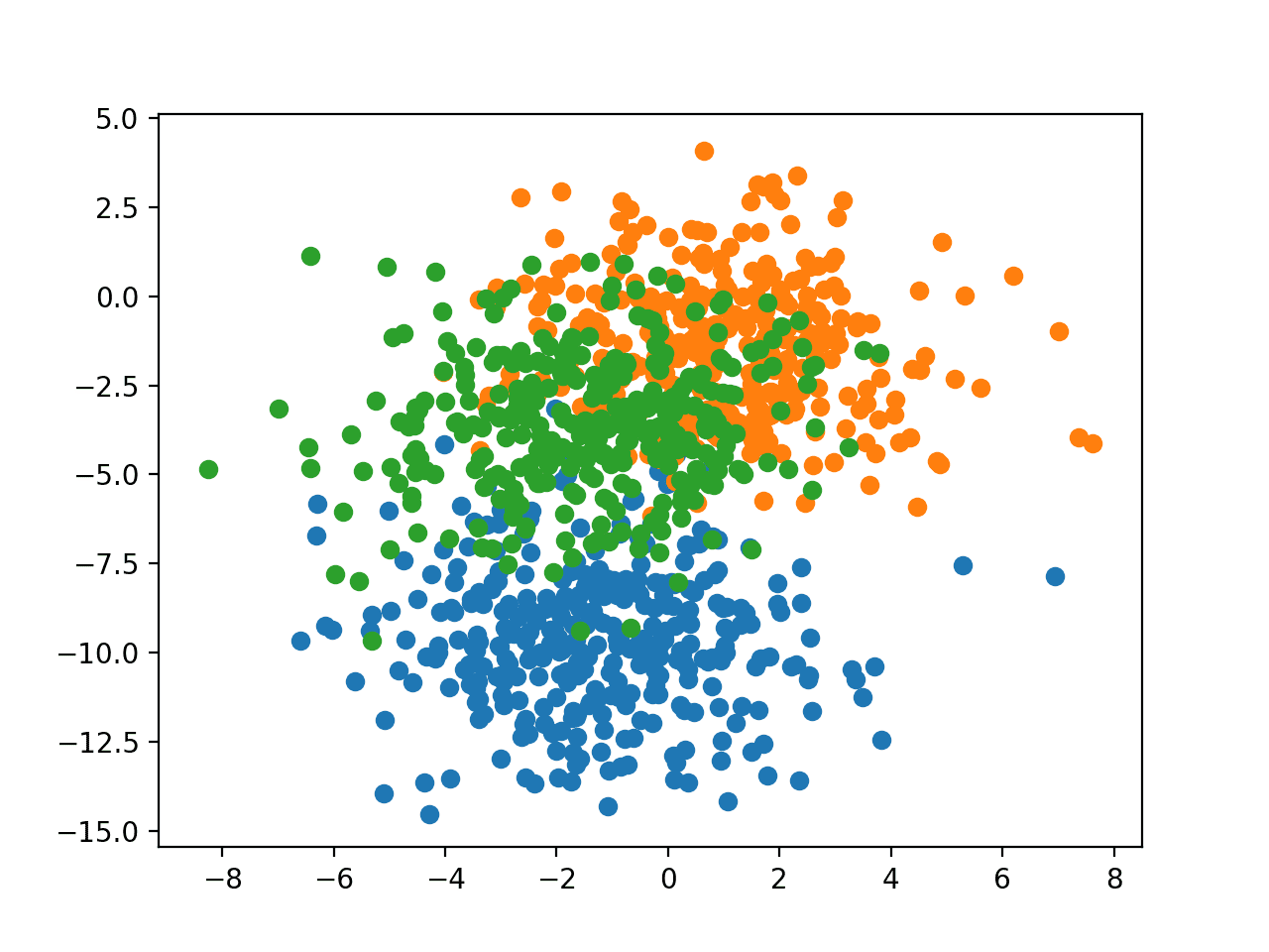
The scikit-learn class provides the make_blobs() function that can be used to create a multi-class classification problem with the prescribed number of samples, input variables, classes, and variance of samples within a class.

The problem will be configured with two input variables (to represent the x and y coordinates of the points) and a standard deviation of 2.0 for points within each group. We will use the same random state (seed for the pseudorandom number generator) to ensure that we always get the same data points.

The results are the input and output elements of a dataset that we can model.

In order to get a feeling for the complexity of the problem, we can plot each point on a two-dimensional scatter plot and color each point by class value.

The complete example is listed below.

Running the example creates a scatter plot of the entire dataset. We can see that the standard deviation of 2.0 means that the classes are not linearly separable (separable by a line), causing many ambiguous points.

This is desirable as it means that the problem is non-trivial and will allow a neural network model to find many different “good enough” candidate solutions.

Scatter Plot of Blobs Dataset With Three Classes and Points Colored by Class Value

Supervised Greedy Layer-Wise Pretraining

In this section, we will use greedy layer-wise supervised learning to build up a deep Multilayer Perceptron (MLP) model for the blobs supervised learning multi-class classification problem.

Pretraining is not required to address this simple predictive modeling problem. Instead, this is a demonstration of how to perform supervised greedy layer-wise pretraining that can be used as a template for larger and more challenging supervised learning problems.

As a first step, we can develop a function to create 1,000 samples from the problem and split them evenly into train and test datasets. The prepare_data() function below implements this and returns the train and test sets in terms of the input and output components.

We can call this function to prepare the data.

Next, we can train and fit a base model.

This will be an MLP that expects two inputs for the two input variables in the dataset and has one hidden layer with 10 nodes and uses the rectified linear activation function. The output layer has three nodes in order to predict the probability for each of the three classes and uses the softmax activation function.

The model is fit using stochastic gradient descent with the sensible default learning rate of 0.01 and a high momentum value of 0.9. The model is optimized using cross entropy loss.

The model is then fit on the training dataset for 100 epochs with a default batch size of 32 examples.

The get_base_model() function below ties these elements together, taking the training dataset as arguments and returning a fit baseline model.

We can call this function to prepare the base model to which we can later add layers one at a time.

We need to be able to easily evaluate the performance of a model on the train and test sets.

The evaluate_model() function below takes the train and test sets as arguments as well as a model and returns the accuracy on both datasets.

We can call this function to calculate and report the accuracy of the base model and store the scores away in a dictionary against the number of layers in the model (currently two, one hidden and one output layer) so we can plot the relationship between layers and accuracy later.

We can now outline the process of greedy layer-wise pretraining.

A function is required that can add a new hidden layer and retrain the model but only update the weights in the newly added layer and in the output layer.

This requires first storing the current output layer including its configuration and current set of weights.

Then removing the output layer from the stack of layers in the model.

All of the remaining layers in the model can then be marked as non-trainable, meaning that their weights cannot be updated when the fit() function is called again.

We can then add a new hidden layer, in this case with the same configuration as the first hidden layer added in the base model.

Finally, the output layer can be added back and the model can be refit on the training dataset.

We can tie all of these elements into a function named add_layer() that takes the model and the training dataset as arguments.

This function can then be called repeatedly based on the number of layers we wish to add to the model.

In this case, we will add 10 layers, one at a time, and evaluate the performance of the model after each additional layer is added to get an idea of how it is impacting performance.

Train and test accuracy scores are stored in the dictionary against the number of layers in the model.

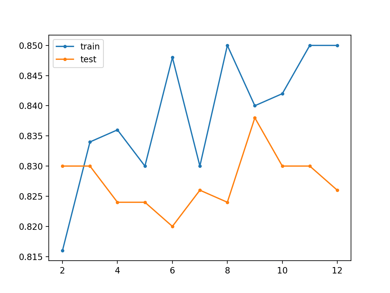
At the end of the run, a line plot is created showing the number of layers in the model (x-axis) compared to the number model accuracy on the train and test datasets.

We would expect the addition of layers to improve the performance of the model on the training dataset and perhaps even on the test dataset.

Tying all of these elements together, the complete example is listed below.

Running the example reports the classification accuracy on the train and test sets for the base model (two layers), then after each additional layer is added (from three to 12 layers).

Note: Your results may vary given the stochastic nature of the algorithm or evaluation procedure, or differences in numerical precision. Consider running the example a few times and compare the average outcome.

In this case, we can see that the baseline model does reasonably well on this problem. As the layers are increased, we can roughly see an increase in accuracy for the model on the training dataset, likely as it is beginning to overfit the data. We see a rough drop in classification accuracy on the test dataset, likely because of the overfitting.

A line plot is also created showing the train (blue) and test set (orange) accuracy as each additional layer is added to the model.

In this case, the plot suggests a slight overfitting of the training dataset, but perhaps better test set performance after seven added layers.

Line Plot for Supervised Greedy Layer-Wise Pretraining Showing Model Layers vs Train and Test Set Classification Accuracy on the Blobs Classification Problem

An interesting extension to this example would be to allow all weights in the model to be fine tuned with a small learning rate for a large number of training epochs to see if this can further reduce generalization error.

Unsupervised Greedy Layer-Wise Pretraining

In this section, we will explore using greedy layer-wise pretraining with an unsupervised model.

Specifically, we will develop an autoencoder model that will be trained to reconstruct input data. In order to use this unsupervised model for classification, we will remove the output layer, add and fit a new output layer for classification.

This is slightly more complex than the previous supervised greedy layer-wise pretraining, but we can reuse many of the same ideas and code from the previous section.

The first step is to define, fit, and evaluate an autoencoder model. We will use the same two-layer base model as we did in the previous section, except modify it to predict the input as the output and use mean squared error to evaluate how good the model is at reconstructing a given input sample.

The base_autoencoder() function below implements this, taking the train and test sets as arguments, then defines, fits, and evaluates the base unsupervised autoencoder model, printing the reconstruction error on the train and test sets and returning the model.

We can call this function in order to prepare our base autoencoder to which we can add and greedily train layers.

Evaluating an autoencoder model on the blobs multi-class classification problem requires a few steps.

The hidden layers will be used as the basis of a classifier with a new output layer that must be trained then used to make predictions before adding back the original output layer so that we can continue to add layers to the autoencoder.

The first step is to reference, then remove the output layer of the autoencoder model.

All of the remaining hidden layers in the autoencoder must be marked as non-trainable so that the weights are not changed when we train the new output layer.

We can now add a new output layer that predicts the probability of an example belonging to reach of the three classes. The model must also be re-compiled using a new loss function suitable for multi-class classification.

The model can then be re-fit on the training dataset, specifically training the output layer on how to make class predictions using the learned features from the autoencoder as input.

The classification accuracy of the fit model can then be evaluated on the train and test datasets.

Finally, we can put the autoencoder back together but removing the classification output layer, adding back the original autoencoder output layer and recompiling the model with an appropriate loss function for reconstruction.

We can tie this together into an evaluate_autoencoder_as_classifier() function that takes the model as well as the train and test sets, then returns the train and test set classification accuracy.

This function can be called to evaluate the baseline autoencoder model and then store the accuracy scores in a dictionary against the number of layers in the model (in this case two).

We are now ready to define the process for adding and pretraining layers to the model.

The process for adding layers is much the same as the supervised case in the previous section, except we are optimizing reconstruction loss rather than classification accuracy for the new layer.

The add_layer_to_autoencoder() function below adds a new hidden layer to the autoencoder model, updates the weights for the new layer and the hidden layers, then reports the reconstruction error on the train and test sets input data. The function does re-mark all prior layers as non-trainable, which is redundant because we already did this in the evaluate_autoencoder_as_classifier() function, but I have left it in, in case you decide to reuse this function in your own project.

We can now repeatedly call this function, adding layers, and evaluating the effect by using the autoencoder as the basis for evaluating a new classifier.

As before, all accuracy scores are collected and we can use them to create a line graph of the number of model layers vs train and test set accuracy.

Tying all of this together, the complete example of unsupervised greedy layer-wise pretraining for the blobs multi-class classification problem is listed below.

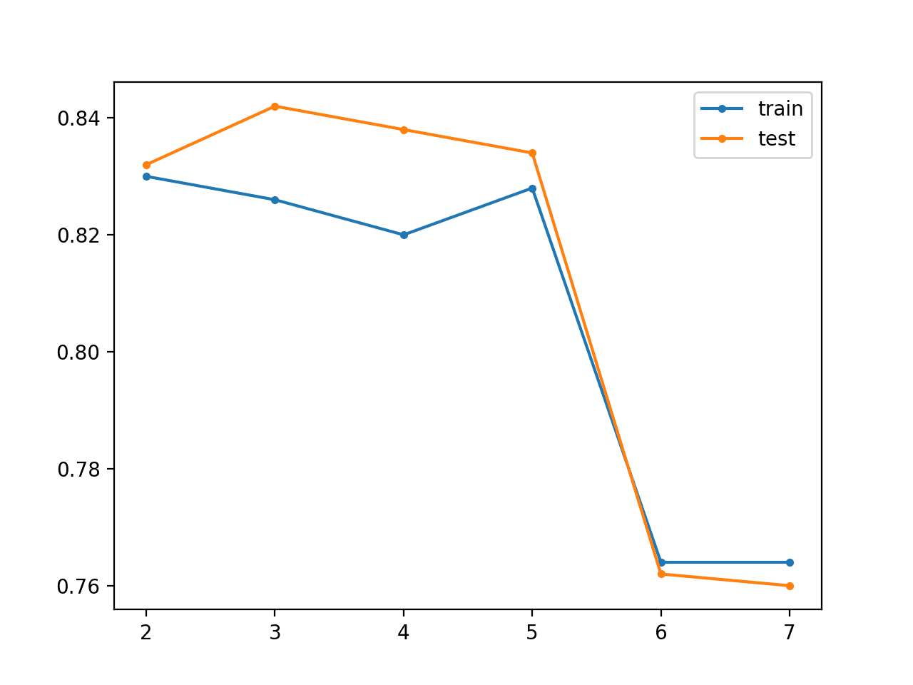
Running the example reports both reconstruction error and classification accuracy on the train and test sets for the model for the base model (two layers) then after each additional layer is added (from three to 12 layers).

Note: Your results may vary given the stochastic nature of the algorithm or evaluation procedure, or differences in numerical precision. Consider running the example a few times and compare the average outcome.

In this case, we can see that reconstruction error starts low, in fact near-perfect, then slowly increases during training. Accuracy on the training dataset seems to decrease as layers are added to the encoder, although accuracy test seems to improve as layers are added, at least until the model has five layers, after which performance appears to crash.

A line plot is also created showing the train (blue) and test set (orange) accuracy as each additional layer is added to the model.

In this case, the plot suggests there may be some minor benefits in the unsupervised greedy layer-wise pretraining, but perhaps beyond five layers the model becomes unstable.

Line Plot for Unsupervised Greedy Layer-Wise Pretraining Showing Model Layers vs Train and Test Set Classification Accuracy on the Blobs Classification Problem

An interesting extension would be to explore whether fine tuning of all weights in the model prior or after fitting a classifier output layer improves performance.

Further Reading

This section provides more resources on the topic if you are looking to go deeper.

Papers

• Greedy Layer-Wise Training of Deep Networks, 2007.
• Why Does Unsupervised Pre-training Help Deep Learning, 2010.

Books

• Section 8.7.4 Supervised Pretraining, Deep Learning, 2016.
• Section 15.1 Greedy Layer-Wise Unsupervised Pretraining, Deep Learning, 2016.

Summary

In this tutorial, you discovered greedy layer-wise pretraining as a technique for developing deep multi-layered neural network models.

Specifically, you learned:

• Greedy layer-wise pretraining provides a way to develop deep multi-layered neural networks whilst only ever training shallow networks.
• Pretraining can be used to iteratively deepen a supervised model or an unsupervised model that can be repurposed as a supervised model.
• Pretraining may be useful for problems with small amounts labeled data and large amounts of unlabeled data.

Do you have any questions?
Ask your questions in the comments below and I will do my best to answer.

Develop Better Deep Learning Models Today!

Train Faster, Reduce Overftting, and Ensembles

...with just a few lines of python code

Discover how in my new Ebook:
Better Deep Learning

It provides self-study tutorials on topics like:
weight decay, batch normalization, dropout, model stacking and much more...

Bring better deep learning to your projects!

Skip the Academics. Just Results.

See What's Inside