How to Fix the Vanishing Gradients Problem Using the ReLU

The vanishing gradients problem is one example of unstable behavior that you may encounter when training a deep neural network.

It describes the situation where a deep multilayer feed-forward network or a recurrent neural network is unable to propagate useful gradient information from the output end of the model back to the layers near the input end of the model.

The result is the general inability of models with many layers to learn on a given dataset, or for models with many layers to prematurely converge to a poor solution.

Many fixes and workarounds have been proposed and investigated, such as alternate weight initialization schemes, unsupervised pre-training, layer-wise training, and variations on gradient descent. Perhaps the most common change is the use of the rectified linear activation function that has become the new default, instead of the hyperbolic tangent activation function that was the default through the late 1990s and 2000s.

In this tutorial, you will discover how to diagnose a vanishing gradient problem when training a neural network model and how to fix it using an alternate activation function and weight initialization scheme.

After completing this tutorial, you will know:

• The vanishing gradients problem limits the development of deep neural networks with classically popular activation functions such as the hyperbolic tangent.
• How to fix a deep neural network Multilayer Perceptron for classification using ReLU and He weight initialization.
• How to use TensorBoard to diagnose a vanishing gradient problem and confirm the impact of ReLU to improve the flow of gradients through the model.

Kick-start your project with my new book Better Deep Learning, including step-by-step tutorials and the Python source code files for all examples.

Let’s get started.

• Updated Oct/2019: Updated for Keras 2.3 and TensorFlow 2.0.

How to Fix the Vanishing Gradient By Using the Rectified Linear Activation Function
Photo by Liam Moloney, some rights reserved.

Tutorial Overview

This tutorial is divided into five parts; they are:

1. Vanishing Gradients Problem
2. Two Circles Binary Classification Problem
3. Multilayer Perceptron Model for Two Circles Problem
4. Deeper MLP Model with ReLU for Two Circles Problem
5. Review Average Gradient Size During Training

Vanishing Gradients Problem

Neural networks are trained using stochastic gradient descent.

This involves first calculating the prediction error made by the model and using the error to estimate a gradient used to update each weight in the network so that less error is made next time. This error gradient is propagated backward through the network from the output layer to the input layer.

It is desirable to train neural networks with many layers, as the addition of more layers increases the capacity of the network, making it capable of learning a large training dataset and efficiently representing more complex mapping functions from inputs to outputs.

A problem with training networks with many layers (e.g. deep neural networks) is that the gradient diminishes dramatically as it is propagated backward through the network. The error may be so small by the time it reaches layers close to the input of the model that it may have very little effect. As such, this problem is referred to as the “vanishing gradients” problem.

Vanishing gradients make it difficult to know which direction the parameters should move to improve the cost function …

— Page 290, Deep Learning, 2016.

In fact, the error gradient can be unstable in deep neural networks and not only vanish, but also explode, where the gradient exponentially increases as it is propagated backward through the network. This is referred to as the “exploding gradient” problem.

The term vanishing gradient refers to the fact that in a feedforward network (FFN) the backpropagated error signal typically decreases (or increases) exponentially as a function of the distance from the final layer.

— Random Walk Initialization for Training Very Deep Feedforward Networks, 2014.

Vanishing gradients is a particular problem with recurrent neural networks as the update of the network involves unrolling the network for each input time step, in effect creating a very deep network that requires weight updates. A modest recurrent neural network may have 200-to-400 input time steps, resulting conceptually in a very deep network.

The vanishing gradients problem may be manifest in a Multilayer Perceptron by a slow rate of improvement of a model during training and perhaps premature convergence, e.g. continued training does not result in any further improvement. Inspecting the changes to the weights during training, we would see more change (i.e. more learning) occurring in the layers closer to the output layer and less change occurring in the layers close to the input layer.

There are many techniques that can be used to reduce the impact of the vanishing gradients problem for feed-forward neural networks, most notably alternate weight initialization schemes and use of alternate activation functions.

Different approaches to training deep networks (both feedforward and recurrent) have been studied and applied [in an effort to address vanishing gradients], such as pre-training, better random initial scaling, better optimization methods, specific architectures, orthogonal initialization, etc.

— Random Walk Initialization for Training Very Deep Feedforward Networks, 2014.

In this tutorial, we will take a closer look at the use of an alternate weight initialization scheme and activation function to permit the training of deeper neural network models.

Two Circles Binary Classification Problem

As the basis for our exploration, we will use a very simple two-class or binary classification problem.

The scikit-learn class provides the make_circles() function that can be used to create a binary classification problem with the prescribed number of samples and statistical noise.

Each example has two input variables that define the x and y coordinates of the point on a two-dimensional plane. The points are arranged in two concentric circles (they have the same center) for the two classes.

The number of points in the dataset is specified by a parameter, half of which will be drawn from each circle. Gaussian noise can be added when sampling the points via the “noise” argument that defines the standard deviation of the noise, where 0.0 indicates no noise or points drawn exactly from the circles. The seed for the pseudorandom number generator can be specified via the “random_state” argument that allows the exact same points to be sampled each time the function is called.

The example below generates 1,000 examples from the two circles with noise and a value of 1 to seed the pseudorandom number generator.

We can create a graph of the dataset, plotting the x and y coordinates of the input variables (X) and coloring each point by the class value (0 or 1).

The complete example is listed below.

Running the example creates a plot showing the 1,000 generated data points with the class value of each point used to color each point.

We can see points for class 0 are blue and represent the outer circle, and points for class 1 are orange and represent the inner circle.

The statistical noise of the generated samples means that there is some overlap of points between the two circles, adding some ambiguity to the problem, making it non-trivial. This is desirable as a neural network may choose one of among many possible solutions to classify the points between the two circles and always make some errors.

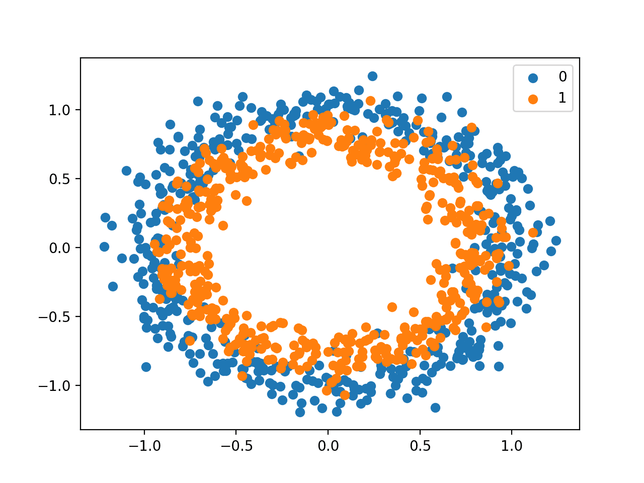
Scatter Plot of Circles Dataset With Points Colored By Class Value

Now that we have defined a problem as the basis for our exploration, we can look at developing a model to address it.

Multilayer Perceptron Model for Two Circles Problem

We can develop a Multilayer Perceptron model to address the two circles problem.

This will be a simple feed-forward neural network model, designed as we were taught in the late 1990s and early 2000s.

First, we will generate 1,000 data points from the two circles problem and rescale the inputs to the range [-1, 1]. The data is almost already in this range, but we will make sure.

Normally, we would prepare the data scaling using a training dataset and apply it to a test dataset. To keep things simple in this tutorial, we will scale all of the data together before splitting it into train and test sets.

Next, we will split the data into train and test sets.

Half of the data will be used for training and the remaining 500 examples will be used as the test set. In this tutorial, the test set will also serve as the validation dataset so we can get an idea of how the model performs on the holdout set during training.

Next, we will define the model.

The model will have an input layer with two inputs, for the two variables in the dataset, one hidden layer with five nodes, and an output layer with one node used to predict the class probability. The hidden layer will use the hyperbolic tangent activation function (tanh) and the output layer will use the logistic activation function (sigmoid) to predict class 0 or class 1 or something in between.

Using the hyperbolic tangent activation function in hidden layers was the best practice in the 1990s and 2000s, performing generally better than the logistic function when used in the hidden layer. It was also good practice to initialize the network weights to small random values from a uniform distribution. Here, we will initialize weights randomly from the range [0.0, 1.0].

The model uses the binary cross entropy loss function and is optimized using stochastic gradient descent with a learning rate of 0.01 and a large momentum of 0.9.

The model is trained for 500 training epochs and the test dataset is evaluated at the end of each epoch along with the training dataset.

After the model is fit, it is evaluated on both the train and test dataset and the accuracy scores are displayed.

Finally, the accuracy of the model during each step of training is graphed as a line plot, showing the dynamics of the model as it learned the problem.

Tying all of this together, the complete example is listed below.

Running the example fits the model in just a few seconds.

Note: Your results may vary given the stochastic nature of the algorithm or evaluation procedure, or differences in numerical precision. Consider running the example a few times and compare the average outcome.

We can see that in this case, the model learned the problem well, achieving an accuracy of about 81.6% on both the train and test datasets.

A line plot of model accuracy on the train and test sets is created, showing the change in performance over all 500 training epochs.

The plot suggests, for this run, that the performance begins to slow around epoch 300 at about 80% accuracy for both the train and test sets.

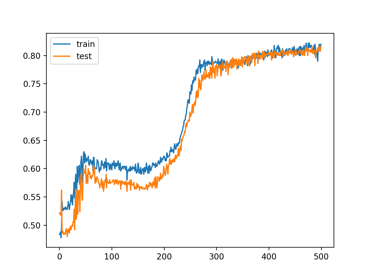
Line Plot of Train and Test Set Accuracy Over Training Epochs for MLP in the Two Circles Problem

Now that we have seen how to develop a classical MLP using the tanh activation function for the two circles problem, we can look at modifying the model to have many more hidden layers.

Deeper MLP Model for Two Circles Problem

Traditionally, developing deep Multilayer Perceptron models was challenging.

Deep models using the hyperbolic tangent activation function do not train easily, and much of this poor performance is blamed on the vanishing gradient problem.

We can attempt to investigate this using the MLP model developed in the previous section.

The number of hidden layers can be increased from 1 to 5; for example:

We can then re-run the example and review the results.

The complete example of the deeper MLP is listed below.

Running the example first prints the performance of the fit model on the train and test datasets.

Note: Your results may vary given the stochastic nature of the algorithm or evaluation procedure, or differences in numerical precision. Consider running the example a few times and compare the average outcome.

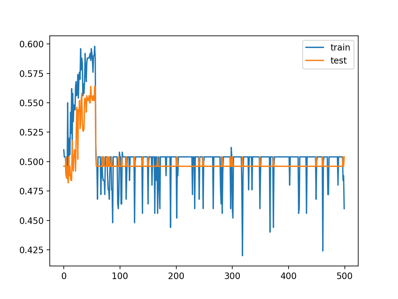
In this case, we can see that performance is quite poor on both the train and test sets achieving around 50% accuracy. This suggests that the model as configured could not learn the problem nor generalize a solution.

The line plots of model accuracy on the train and test sets during training tell a similar story. We can see that performance is bad and actually gets worse as training progresses.

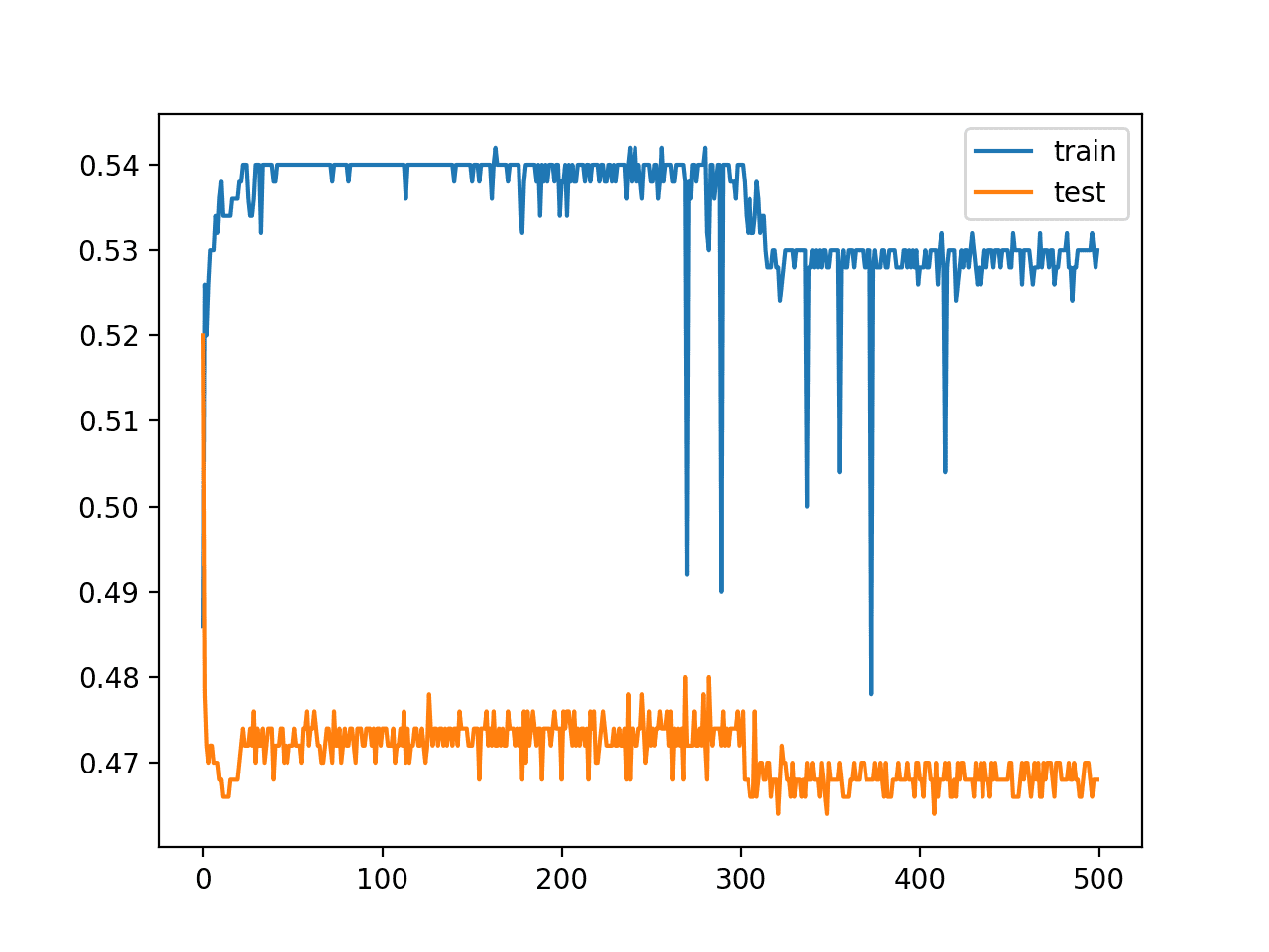
Line Plot of Train and Test Set Accuracy of Over Training Epochs for Deep MLP in the Two Circles Problem

Deeper MLP Model with ReLU for Two Circles Problem

The rectified linear activation function has supplanted the hyperbolic tangent activation function as the new preferred default when developing Multilayer Perceptron networks, as well as other network types like CNNs.

This is because the activation function looks and acts like a linear function, making it easier to train and less likely to saturate, but is, in fact, a nonlinear function, forcing negative inputs to the value 0. It is claimed as one possible approach to addressing the vanishing gradients problem when training deeper models.

When using the rectified linear activation function (or ReLU for short), it is good practice to use the He weight initialization scheme. We can define the MLP with five hidden layers using ReLU and He initialization, listed below.

Tying this together, the complete code example is listed below.

Running the example prints the performance of the model on the train and test datasets.

Note: Your results may vary given the stochastic nature of the algorithm or evaluation procedure, or differences in numerical precision. Consider running the example a few times and compare the average outcome.

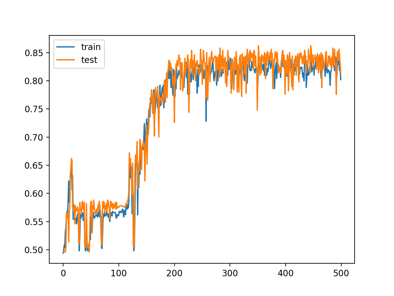
In this case, we can see that this small change has allowed the model to learn the problem, achieving about 84% accuracy on both datasets, outperforming the single layer model using the tanh activation function.

A line plot of model accuracy on the train and test sets over training epochs is also created. The plot shows quite different dynamics to what we have seen so far.

The model appears to rapidly learn the problem, converging on a solution in about 100 epochs.

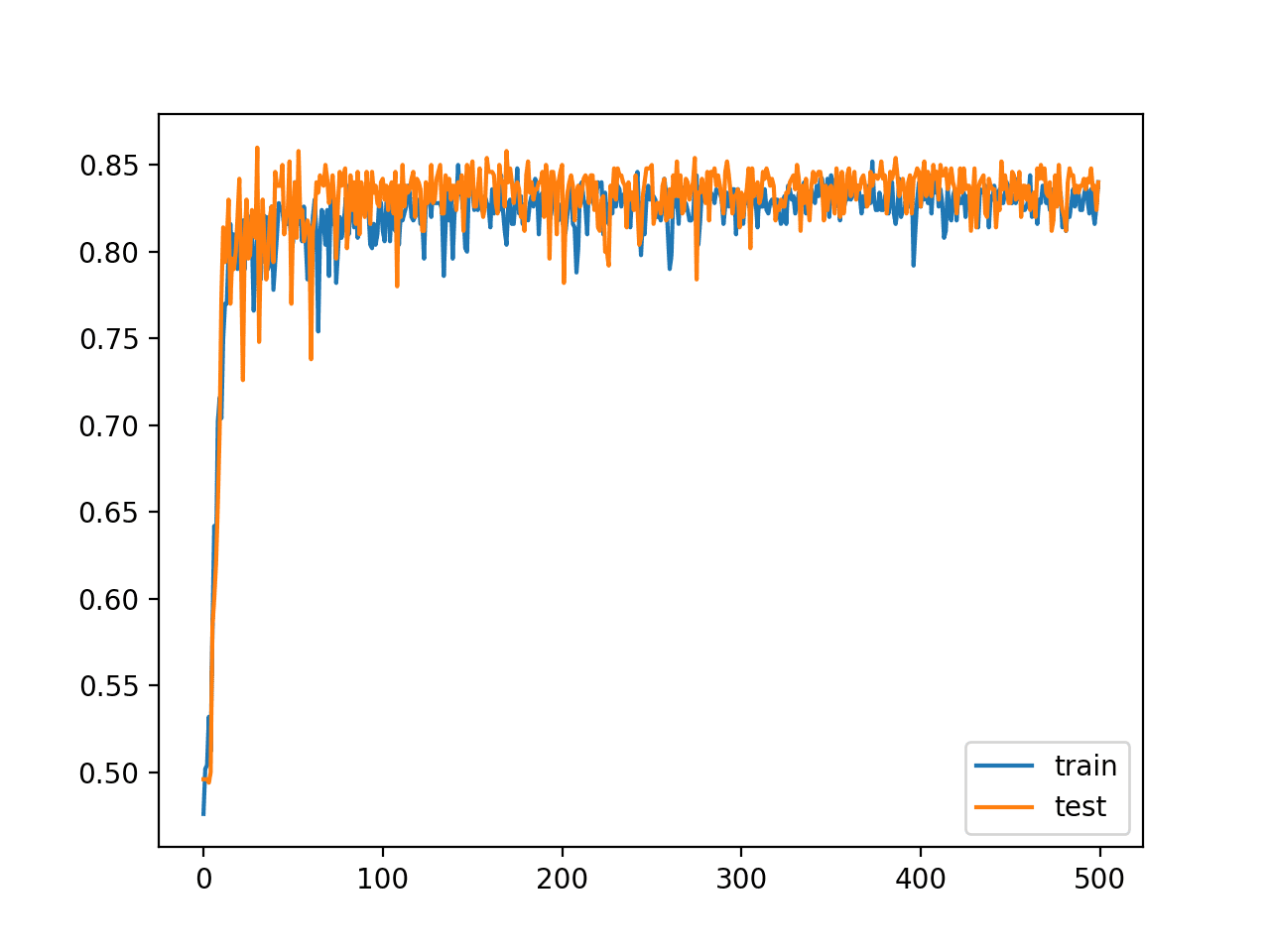
Line Plot of Train and Test Set Accuracy of Over Training Epochs for Deep MLP with ReLU in the Two Circles Problem

Use of the ReLU activation function has allowed us to fit a much deeper model for this simple problem, but this capability does not extend infinitely. For example, increasing the number of layers results in slower learning to a point at about 20 layers where the model is no longer capable of learning the problem, at least with the chosen configuration.

For example, below is a line plot of train and test accuracy of the same model with 15 hidden layers that shows that it is still capable of learning the problem.

Line Plot of Train and Test Set Accuracy of Over Training Epochs for Deep MLP with ReLU with 15 Hidden Layers

Below is a line plot of train and test accuracy over epochs with the same model with 20 layers, showing that the configuration is no longer capable of learning the problem.

Line Plot of Train and Test Set Accuracy of Over Training Epochs for Deep MLP with ReLU with 20 Hidden Layers

Although use of the ReLU worked, we cannot be confident that use of the tanh function failed because of vanishing gradients and ReLU succeed because it overcame this problem.

Review Average Gradient Size During Training

This section assumes that you are using the TensorFlow backend with Keras. If this is not the case, you can skip this section.

In the cases of using the tanh activation function, we know the network has more than enough capacity to learn the problem, but the increase in layers has prevented it from doing so.

It is hard to diagnose a vanishing gradient as a cause for bad performance. One possible signal is to review the average size of the gradient per layer per training epoch.

We would expect layers closer to the output to have a larger average gradient than those layers closer to the input.

Keras provides the TensorBoard callback that can be used to log properties of the model during training such as the average gradient per layer. These statistics can then be reviewed using the TensorBoard interface that is provided with TensorFlow.

We can configure this callback to record the average gradient per-layer per-training epoch, then ensure the callback is used as part of training the model.

We can use this callback to first investigate the dynamics of the gradients in the deep model fit using the hyperbolic tangent activation function, then later compare the dynamics to the same model fit using the rectified linear activation function.

First, the complete example of the deep MLP model using tanh and the TensorBoard callback is listed below.

Running the example creates a new “logs/” subdirectory with a file containing the statistics recorded by the callback during training.

We can review the statistics in the TensorBoard web interface. The interface can be started from the command line, requiring that you specify the full path to your logs directory.

For example, if you run the code in a “/code” directory, then the full path to the logs directory will be “/code/logs/“.

Below is the command to start the TensorBoard interface to be executed on your command line (command prompt). Be sure to change the path to your logs directory.

Next, open your web browser and enter the following URL:

• http://localhost:6006

If all went well, you will see the TensorBoard web interface.

Plots of the average gradient per layer per training epoch can be reviewed under the “Distributions” and “Histograms” tabs of the interface. The plots can be filtered to only show the gradients for the Dense layers, excluding the bias, using the search filter “kernel_0_grad“.

Note: Your results may vary given the stochastic nature of the algorithm or evaluation procedure, or differences in numerical precision. Consider running the example a few times and compare the average outcome.

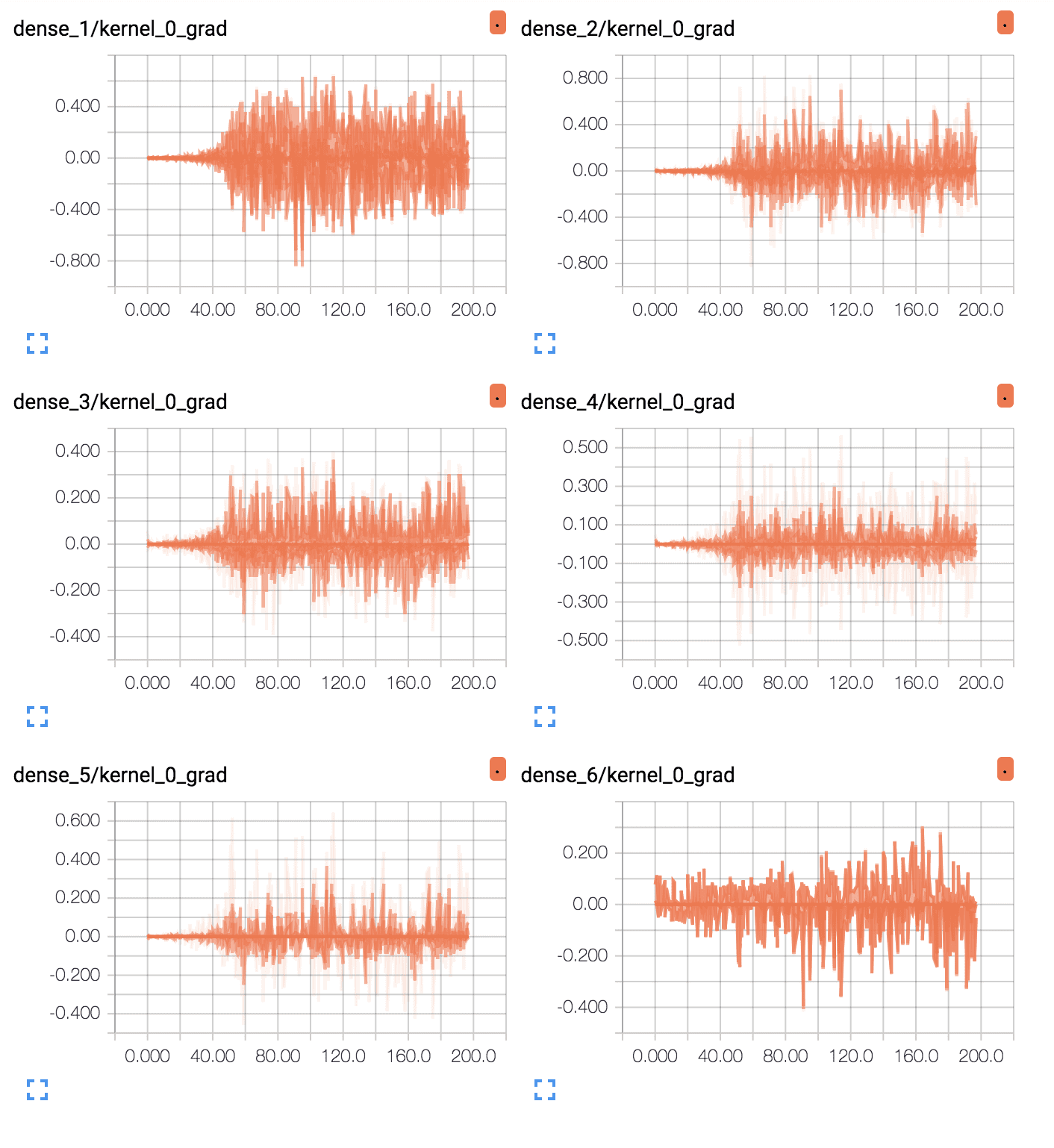
First, line plots are created for each of the 6 layers (5 hidden, 1 output). The names of the plots indicate the layer, where “dense_1” indicates the hidden layer after the input layer and “dense_6” represents the output layer.

We can see that the output layer has a lot of activity over the entire run, with average gradients per epoch at around 0.05 to 0.1. We can also see some activity in the first hidden layer with a similar range. Therefore, gradients are getting through to the first hidden layer, but the last layer and last hidden layer is seeing most of the activity.

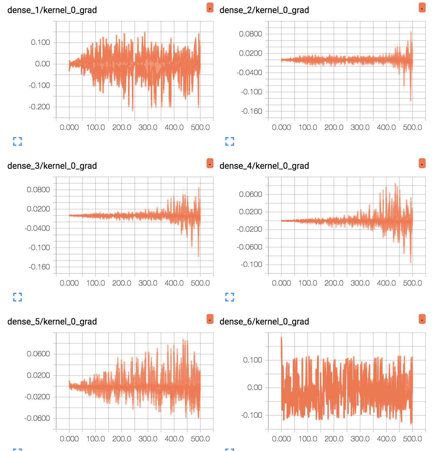
TensorBoard Line Plots of Average Gradients Per Layer for Deep MLP With Tanh

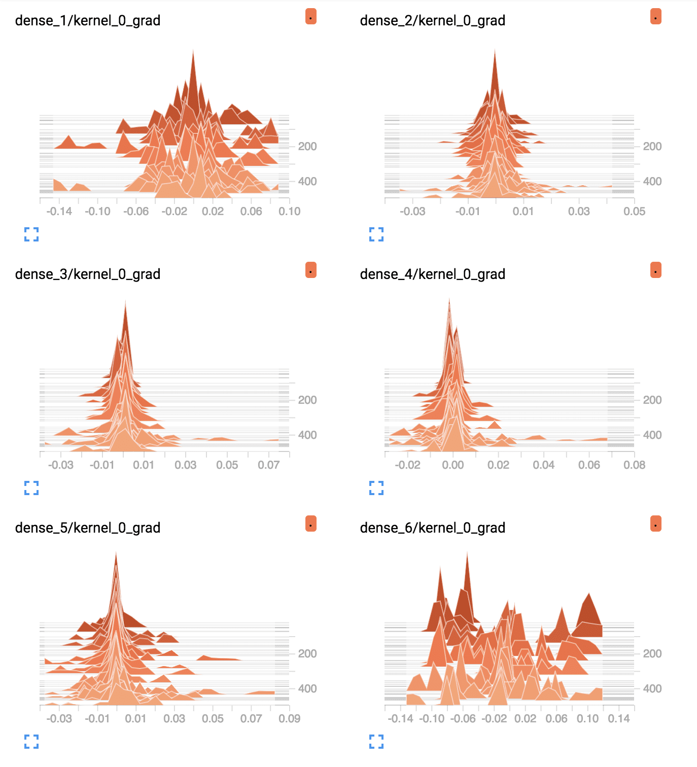
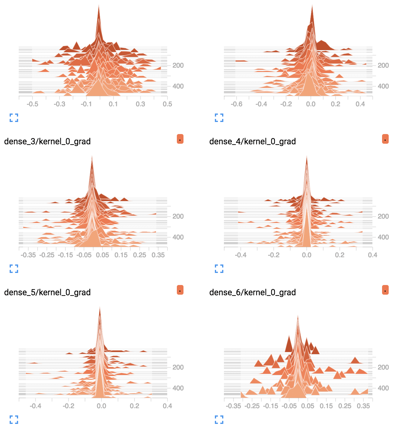
TensorBoard Density Plots of Average Gradients Per Layer for Deep MLP With Tanh

We can collect the same information from the deep MLP with the ReLU activation function.

The complete example is listed below.

The TensorBoard interface can be confusing if you are new to it.

To keep things simple, delete the “logs” subdirectory prior to running this second example.

Once run, you can start the TensorBoard interface the same way and access it through your web browser.

The plots of the average gradient per layer per training epoch show a different story as compared to the gradients for the deep model with tanh.

We can see that the first hidden layer sees more gradients, more consistently with larger spread, perhaps 0.2 to 0.4, as opposed to 0.05 and 0.1 seen with tanh. We can also see that the middle hidden layers see large gradients.

TensorBoard Line Plots of Average Gradients Per Layer for Deep MLP With ReLU

TensorBoard Density Plots of Average Gradients Per Layer for Deep MLP With ReLU

The ReLU activation function is allowing more gradient to flow backward through the model during training, and this may be the cause for improved performance.

Extensions

This section lists some ideas for extending the tutorial that you may wish to explore.

• Weight Initialization. Update the deep MLP with tanh activation to use Xavier uniform weight initialization and report the results.
• Learning Algorithm. Update the deep MLP with tanh activation to use an adaptive learning algorithm such as Adam and report the results.
• Weight Changes. Update the tanh and relu examples to record and plot the L1 vector norm of model weights each epoch as a proxy for how much each layer is changed during training and compare results.
• Study Model Depth. Create an experiment using the MLP with tanh activation and report the performance of models as the number of hidden layers is increased from 1 to 10.
• Increase Breadth. Increase the number of nodes in the hidden layers of the MLP with tanh activation from 5 to 25 and report performance as the number of layers are increased from 1 to 10.

If you explore any of these extensions, I’d love to know.

Further Reading

This section provides more resources on the topic if you are looking to go deeper.

Posts

• A Gentle Introduction to the Rectified Linear Activation Unit (ReLU) for Deep Learning Neural Networks

Papers

• Random Walk Initialization for Training Very Deep Feedforward Networks, 2014.
• Gradient Flow in Recurrent Nets: the Difficulty of Learning Long-Term Dependencies, 2001.

Books

• Section 8.2.5 Long-Term Dependencies, Deep Learning, 2016.
• Chapter 5 Why are deep neural networks hard to train?, Neural Networks and Deep Learning.

API

• RandomUniform Keras Weight Initialization API
• SGD Keras Optimizer API
• TensorBoard Keras Callback API
• TensorFlow TensorBoard Guide

Articles

• Vanishing gradient problem, Wikipedia.

Summary

In this tutorial, you discovered how to diagnose a vanishing gradient problem when training a neural network model and how to fix it using an alternate activation function and weight initialization scheme.

Specifically, you learned:

• The vanishing gradients problem limits the development of deep neural networks with classically popular activation functions such as the hyperbolic tangent.
• How to fix a deep neural network Multilayer Perceptron for classification using ReLU and He weight initialization.
• How to use TensorBoard to diagnose a vanishing gradient problem and confirm the impact of ReLU to improve the flow of gradients through the model.

Do you have any questions?
Ask your questions in the comments below and I will do my best to answer.

Develop Better Deep Learning Models Today!

Train Faster, Reduce Overftting, and Ensembles

...with just a few lines of python code

Discover how in my new Ebook:
Better Deep Learning

It provides self-study tutorials on topics like:
weight decay, batch normalization, dropout, model stacking and much more...

Bring better deep learning to your projects!

Skip the Academics. Just Results.

See What's Inside