Deep learning neural networks are trained using the stochastic gradient descent optimization algorithm.
As part of the optimization algorithm, the error for the current state of the model must be estimated repeatedly. This requires the choice of an error function, conventionally called a loss function, that can be used to estimate the loss of the model so that the weights can be updated to reduce the loss on the next evaluation.
Neural network models learn a mapping from inputs to outputs from examples and the choice of loss function must match the framing of the specific predictive modeling problem, such as classification or regression. Further, the configuration of the output layer must also be appropriate for the chosen loss function.
In this tutorial, you will discover how to choose a loss function for your deep learning neural network for a given predictive modeling problem.
After completing this tutorial, you will know:
- How to configure a model for mean squared error and variants for regression problems.
- How to configure a model for cross-entropy and hinge loss functions for binary classification.
- How to configure a model for cross-entropy and KL divergence loss functions for multi-class classification.
Kick-start your project with my new book Better Deep Learning, including step-by-step tutorials and the Python source code files for all examples.
Let’s get started.
- Update Oct/2019: Updated for Keras 2.3 and TensorFlow 2.0.
- Update Jan/2020: Updated for changes in scikit-learn v0.22 API

How to Choose Loss Functions When Training Deep Learning Neural Networks
Photo by GlacierNPS, some rights reserved.
Tutorial Overview
This tutorial is divided into three parts; they are:
- Regression Loss Functions
- Mean Squared Error Loss
- Mean Squared Logarithmic Error Loss
- Mean Absolute Error Loss
- Binary Classification Loss Functions
- Binary Cross-Entropy
- Hinge Loss
- Squared Hinge Loss
- Multi-Class Classification Loss Functions
- Multi-Class Cross-Entropy Loss
- Sparse Multiclass Cross-Entropy Loss
- Kullback Leibler Divergence Loss
We will focus on how to choose and implement different loss functions.
For more theory on loss functions, see the post:
Regression Loss Functions
A regression predictive modeling problem involves predicting a real-valued quantity.
In this section, we will investigate loss functions that are appropriate for regression predictive modeling problems.
As the context for this investigation, we will use a standard regression problem generator provided by the scikit-learn library in the make_regression() function. This function will generate examples from a simple regression problem with a given number of input variables, statistical noise, and other properties.
We will use this function to define a problem that has 20 input features; 10 of the features will be meaningful and 10 will not be relevant. A total of 1,000 examples will be randomly generated. The pseudorandom number generator will be fixed to ensure that we get the same 1,000 examples each time the code is run.
|
1 2 |
# generate regression dataset X, y = make_regression(n_samples=1000, n_features=20, noise=0.1, random_state=1) |
Neural networks generally perform better when the real-valued input and output variables are to be scaled to a sensible range. For this problem, each of the input variables and the target variable have a Gaussian distribution; therefore, standardizing the data in this case is desirable.
We can achieve this using the StandardScaler transformer class also from the scikit-learn library. On a real problem, we would prepare the scaler on the training dataset and apply it to the train and test sets, but for simplicity, we will scale all of the data together before splitting into train and test sets.
|
1 2 3 |
# standardize dataset X = StandardScaler().fit_transform(X) y = StandardScaler().fit_transform(y.reshape(len(y),1))[:,0] |
Once scaled, the data will be split evenly into train and test sets.
|
1 2 3 4 |
# split into train and test n_train = 500 trainX, testX = X[:n_train, :], X[n_train:, :] trainy, testy = y[:n_train], y[n_train:] |
A small Multilayer Perceptron (MLP) model will be defined to address this problem and provide the basis for exploring different loss functions.
The model will expect 20 features as input as defined by the problem. The model will have one hidden layer with 25 nodes and will use the rectified linear activation function (ReLU). The output layer will have 1 node, given the one real-value to be predicted, and will use the linear activation function.
|
1 2 3 4 |
# define model model = Sequential() model.add(Dense(25, input_dim=20, activation='relu', kernel_initializer='he_uniform')) model.add(Dense(1, activation='linear')) |
The model will be fit with stochastic gradient descent with a learning rate of 0.01 and a momentum of 0.9, both sensible default values.
Training will be performed for 100 epochs and the test set will be evaluated at the end of each epoch so that we can plot learning curves at the end of the run.
|
1 2 3 4 |
opt = SGD(lr=0.01, momentum=0.9) model.compile(loss='...', optimizer=opt) # fit model history = model.fit(trainX, trainy, validation_data=(testX, testy), epochs=100, verbose=0) |
Now that we have the basis of a problem and model, we can take a look evaluating three common loss functions that are appropriate for a regression predictive modeling problem.
Although an MLP is used in these examples, the same loss functions can be used when training CNN and RNN models for regression.
Want Better Results with Deep Learning?
Take my free 7-day email crash course now (with sample code).
Click to sign-up and also get a free PDF Ebook version of the course.
Mean Squared Error Loss
The Mean Squared Error, or MSE, loss is the default loss to use for regression problems.
Mathematically, it is the preferred loss function under the inference framework of maximum likelihood if the distribution of the target variable is Gaussian. It is the loss function to be evaluated first and only changed if you have a good reason.
Mean squared error is calculated as the average of the squared differences between the predicted and actual values. The result is always positive regardless of the sign of the predicted and actual values and a perfect value is 0.0. The squaring means that larger mistakes result in more error than smaller mistakes, meaning that the model is punished for making larger mistakes.
The mean squared error loss function can be used in Keras by specifying ‘mse‘ or ‘mean_squared_error‘ as the loss function when compiling the model.
|
1 |
model.compile(loss='mean_squared_error') |
It is recommended that the output layer has one node for the target variable and the linear activation function is used.
|
1 |
model.add(Dense(1, activation='linear')) |
A complete example of demonstrating an MLP on the described regression problem is listed below.
|
1 2 3 4 5 6 7 8 9 10 11 12 13 14 15 16 17 18 19 20 21 22 23 24 25 26 27 28 29 30 31 32 33 34 |
# mlp for regression with mse loss function from sklearn.datasets import make_regression from sklearn.preprocessing import StandardScaler from keras.models import Sequential from keras.layers import Dense from keras.optimizers import SGD from matplotlib import pyplot # generate regression dataset X, y = make_regression(n_samples=1000, n_features=20, noise=0.1, random_state=1) # standardize dataset X = StandardScaler().fit_transform(X) y = StandardScaler().fit_transform(y.reshape(len(y),1))[:,0] # split into train and test n_train = 500 trainX, testX = X[:n_train, :], X[n_train:, :] trainy, testy = y[:n_train], y[n_train:] # define model model = Sequential() model.add(Dense(25, input_dim=20, activation='relu', kernel_initializer='he_uniform')) model.add(Dense(1, activation='linear')) opt = SGD(lr=0.01, momentum=0.9) model.compile(loss='mean_squared_error', optimizer=opt) # fit model history = model.fit(trainX, trainy, validation_data=(testX, testy), epochs=100, verbose=0) # evaluate the model train_mse = model.evaluate(trainX, trainy, verbose=0) test_mse = model.evaluate(testX, testy, verbose=0) print('Train: %.3f, Test: %.3f' % (train_mse, test_mse)) # plot loss during training pyplot.title('Loss / Mean Squared Error') pyplot.plot(history.history['loss'], label='train') pyplot.plot(history.history['val_loss'], label='test') pyplot.legend() pyplot.show() |
Running the example first prints the mean squared error for the model on the train and test datasets.
Note: Your results may vary given the stochastic nature of the algorithm or evaluation procedure, or differences in numerical precision. Consider running the example a few times and compare the average outcome.
In this case, we can see that the model learned the problem achieving zero error, at least to three decimal places.
|
1 |
Train: 0.000, Test: 0.001 |
A line plot is also created showing the mean squared error loss over the training epochs for both the train (blue) and test (orange) sets.
We can see that the model converged reasonably quickly and both train and test performance remained equivalent. The performance and convergence behavior of the model suggest that mean squared error is a good match for a neural network learning this problem.
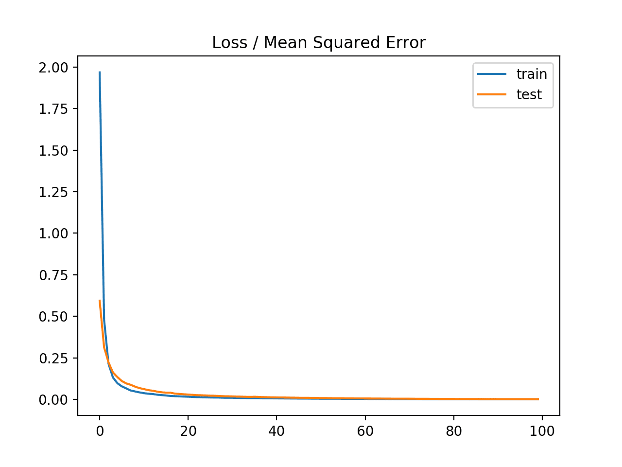
Line plot of Mean Squared Error Loss over Training Epochs When Optimizing the Mean Squared Error Loss Function
Mean Squared Logarithmic Error Loss
There may be regression problems in which the target value has a spread of values and when predicting a large value, you may not want to punish a model as heavily as mean squared error.
Instead, you can first calculate the natural logarithm of each of the predicted values, then calculate the mean squared error. This is called the Mean Squared Logarithmic Error loss, or MSLE for short.
It has the effect of relaxing the punishing effect of large differences in large predicted values.
As a loss measure, it may be more appropriate when the model is predicting unscaled quantities directly. Nevertheless, we can demonstrate this loss function using our simple regression problem.
The model can be updated to use the ‘mean_squared_logarithmic_error‘ loss function and keep the same configuration for the output layer. We will also track the mean squared error as a metric when fitting the model so that we can use it as a measure of performance and plot the learning curve.
|
1 |
model.compile(loss='mean_squared_logarithmic_error', optimizer=opt, metrics=['mse']) |
The complete example of using the MSLE loss function is listed below.
|
1 2 3 4 5 6 7 8 9 10 11 12 13 14 15 16 17 18 19 20 21 22 23 24 25 26 27 28 29 30 31 32 33 34 35 36 37 38 39 40 41 |
# mlp for regression with msle loss function from sklearn.datasets import make_regression from sklearn.preprocessing import StandardScaler from keras.models import Sequential from keras.layers import Dense from keras.optimizers import SGD from matplotlib import pyplot # generate regression dataset X, y = make_regression(n_samples=1000, n_features=20, noise=0.1, random_state=1) # standardize dataset X = StandardScaler().fit_transform(X) y = StandardScaler().fit_transform(y.reshape(len(y),1))[:,0] # split into train and test n_train = 500 trainX, testX = X[:n_train, :], X[n_train:, :] trainy, testy = y[:n_train], y[n_train:] # define model model = Sequential() model.add(Dense(25, input_dim=20, activation='relu', kernel_initializer='he_uniform')) model.add(Dense(1, activation='linear')) opt = SGD(lr=0.01, momentum=0.9) model.compile(loss='mean_squared_logarithmic_error', optimizer=opt, metrics=['mse']) # fit model history = model.fit(trainX, trainy, validation_data=(testX, testy), epochs=100, verbose=0) # evaluate the model _, train_mse = model.evaluate(trainX, trainy, verbose=0) _, test_mse = model.evaluate(testX, testy, verbose=0) print('Train: %.3f, Test: %.3f' % (train_mse, test_mse)) # plot loss during training pyplot.subplot(211) pyplot.title('Loss') pyplot.plot(history.history['loss'], label='train') pyplot.plot(history.history['val_loss'], label='test') pyplot.legend() # plot mse during training pyplot.subplot(212) pyplot.title('Mean Squared Error') pyplot.plot(history.history['mean_squared_error'], label='train') pyplot.plot(history.history['val_mean_squared_error'], label='test') pyplot.legend() pyplot.show() |
Running the example first prints the mean squared error for the model on the train and test dataset.
Note: Your results may vary given the stochastic nature of the algorithm or evaluation procedure, or differences in numerical precision. Consider running the example a few times and compare the average outcome.
In this case, we can see that the model resulted in slightly worse MSE on both the training and test dataset. It may not be a good fit for this problem as the distribution of the target variable is a standard Gaussian.
|
1 |
Train: 0.165, Test: 0.184 |
A line plot is also created showing the mean squared logarithmic error loss over the training epochs for both the train (blue) and test (orange) sets (top), and a similar plot for the mean squared error (bottom).
We can see that the MSLE converged well over the 100 epochs algorithm; it appears that the MSE may be showing signs of overfitting the problem, dropping fast and starting to rise from epoch 20 onwards.
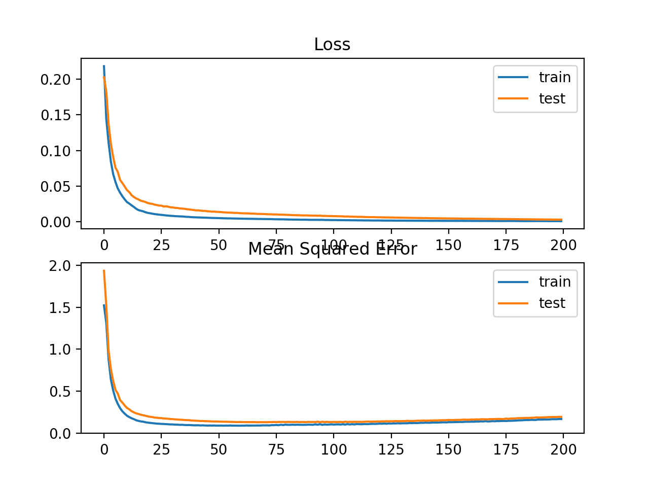
Line Plots of Mean Squared Logarithmic Error Loss and Mean Squared Error Over Training Epochs
Mean Absolute Error Loss
On some regression problems, the distribution of the target variable may be mostly Gaussian, but may have outliers, e.g. large or small values far from the mean value.
The Mean Absolute Error, or MAE, loss is an appropriate loss function in this case as it is more robust to outliers. It is calculated as the average of the absolute difference between the actual and predicted values.
The model can be updated to use the ‘mean_absolute_error‘ loss function and keep the same configuration for the output layer.
|
1 |
model.compile(loss='mean_absolute_error', optimizer=opt, metrics=['mse']) |
The complete example using the mean absolute error as the loss function on the regression test problem is listed below.
|
1 2 3 4 5 6 7 8 9 10 11 12 13 14 15 16 17 18 19 20 21 22 23 24 25 26 27 28 29 30 31 32 33 34 35 36 37 38 39 40 41 |
# mlp for regression with mae loss function from sklearn.datasets import make_regression from sklearn.preprocessing import StandardScaler from keras.models import Sequential from keras.layers import Dense from keras.optimizers import SGD from matplotlib import pyplot # generate regression dataset X, y = make_regression(n_samples=1000, n_features=20, noise=0.1, random_state=1) # standardize dataset X = StandardScaler().fit_transform(X) y = StandardScaler().fit_transform(y.reshape(len(y),1))[:,0] # split into train and test n_train = 500 trainX, testX = X[:n_train, :], X[n_train:, :] trainy, testy = y[:n_train], y[n_train:] # define model model = Sequential() model.add(Dense(25, input_dim=20, activation='relu', kernel_initializer='he_uniform')) model.add(Dense(1, activation='linear')) opt = SGD(lr=0.01, momentum=0.9) model.compile(loss='mean_absolute_error', optimizer=opt, metrics=['mse']) # fit model history = model.fit(trainX, trainy, validation_data=(testX, testy), epochs=100, verbose=0) # evaluate the model _, train_mse = model.evaluate(trainX, trainy, verbose=0) _, test_mse = model.evaluate(testX, testy, verbose=0) print('Train: %.3f, Test: %.3f' % (train_mse, test_mse)) # plot loss during training pyplot.subplot(211) pyplot.title('Loss') pyplot.plot(history.history['loss'], label='train') pyplot.plot(history.history['val_loss'], label='test') pyplot.legend() # plot mse during training pyplot.subplot(212) pyplot.title('Mean Squared Error') pyplot.plot(history.history['mean_squared_error'], label='train') pyplot.plot(history.history['val_mean_squared_error'], label='test') pyplot.legend() pyplot.show() |
Running the example first prints the mean squared error for the model on the train and test dataset.
Note: Your results may vary given the stochastic nature of the algorithm or evaluation procedure, or differences in numerical precision. Consider running the example a few times and compare the average outcome.
In this case, we can see that the model learned the problem, achieving a near zero error, at least to three decimal places.
|
1 |
Train: 0.002, Test: 0.002 |
A line plot is also created showing the mean absolute error loss over the training epochs for both the train (blue) and test (orange) sets (top), and a similar plot for the mean squared error (bottom).
In this case, we can see that MAE does converge but shows a bumpy course, although the dynamics of MSE don’t appear greatly affected. We know that the target variable is a standard Gaussian with no large outliers, so MAE would not be a good fit in this case.
It might be more appropriate on this problem if we did not scale the target variable first.
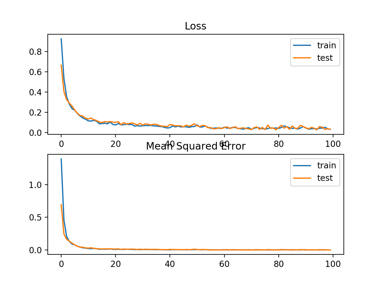
Line plots of Mean Absolute Error Loss and Mean Squared Error over Training Epochs
Binary Classification Loss Functions
Binary classification are those predictive modeling problems where examples are assigned one of two labels.
The problem is often framed as predicting a value of 0 or 1 for the first or second class and is often implemented as predicting the probability of the example belonging to class value 1.
In this section, we will investigate loss functions that are appropriate for binary classification predictive modeling problems.
We will generate examples from the circles test problem in scikit-learn as the basis for this investigation. The circles problem involves samples drawn from two concentric circles on a two-dimensional plane, where points on the outer circle belong to class 0 and points for the inner circle belong to class 1. Statistical noise is added to the samples to add ambiguity and make the problem more challenging to learn.
We will generate 1,000 examples and add 10% statistical noise. The pseudorandom number generator will be seeded with the same value to ensure that we always get the same 1,000 examples.
|
1 2 |
# generate circles X, y = make_circles(n_samples=1000, noise=0.1, random_state=1) |
We can create a scatter plot of the dataset to get an idea of the problem we are modeling. The complete example is listed below.
|
1 2 3 4 5 6 7 8 9 10 11 12 |
# scatter plot of the circles dataset with points colored by class from sklearn.datasets import make_circles from numpy import where from matplotlib import pyplot # generate circles X, y = make_circles(n_samples=1000, noise=0.1, random_state=1) # select indices of points with each class label for i in range(2): samples_ix = where(y == i) pyplot.scatter(X[samples_ix, 0], X[samples_ix, 1], label=str(i)) pyplot.legend() pyplot.show() |
Running the example creates a scatter plot of the examples, where the input variables define the location of the point and the class value defines the color, with class 0 blue and class 1 orange.

Scatter Plot of Dataset for the Circles Binary Classification Problem
The points are already reasonably scaled around 0, almost in [-1,1]. We won’t rescale them in this case.
The dataset is split evenly for train and test sets.
|
1 2 3 4 |
# split into train and test n_train = 500 trainX, testX = X[:n_train, :], X[n_train:, :] trainy, testy = y[:n_train], y[n_train:] |
A simple MLP model can be defined to address this problem that expects two inputs for the two features in the dataset, a hidden layer with 50 nodes, a rectified linear activation function and an output layer that will need to be configured for the choice of loss function.
|
1 2 3 4 |
# define model model = Sequential() model.add(Dense(50, input_dim=2, activation='relu', kernel_initializer='he_uniform')) model.add(Dense(1, activation='...')) |
The model will be fit using stochastic gradient descent with the sensible default learning rate of 0.01 and momentum of 0.9.
|
1 2 |
opt = SGD(lr=0.01, momentum=0.9) model.compile(loss='...', optimizer=opt, metrics=['accuracy']) |
We will fit the model for 200 training epochs and evaluate the performance of the model against the loss and accuracy at the end of each epoch so that we can plot learning curves.
|
1 2 |
# fit model history = model.fit(trainX, trainy, validation_data=(testX, testy), epochs=200, verbose=0) |
Now that we have the basis of a problem and model, we can take a look evaluating three common loss functions that are appropriate for a binary classification predictive modeling problem.
Although an MLP is used in these examples, the same loss functions can be used when training CNN and RNN models for binary classification.
Binary Cross-Entropy Loss
Cross-entropy is the default loss function to use for binary classification problems.
It is intended for use with binary classification where the target values are in the set {0, 1}.
Mathematically, it is the preferred loss function under the inference framework of maximum likelihood. It is the loss function to be evaluated first and only changed if you have a good reason.
Cross-entropy will calculate a score that summarizes the average difference between the actual and predicted probability distributions for predicting class 1. The score is minimized and a perfect cross-entropy value is 0.
Cross-entropy can be specified as the loss function in Keras by specifying ‘binary_crossentropy‘ when compiling the model.
|
1 |
model.compile(loss='binary_crossentropy', optimizer=opt, metrics=['accuracy']) |
The function requires that the output layer is configured with a single node and a ‘sigmoid‘ activation in order to predict the probability for class 1.
|
1 |
model.add(Dense(1, activation='sigmoid')) |
The complete example of an MLP with cross-entropy loss for the two circles binary classification problem is listed below.
|
1 2 3 4 5 6 7 8 9 10 11 12 13 14 15 16 17 18 19 20 21 22 23 24 25 26 27 28 29 30 31 32 33 34 35 36 37 |
# mlp for the circles problem with cross entropy loss from sklearn.datasets import make_circles from keras.models import Sequential from keras.layers import Dense from keras.optimizers import SGD from matplotlib import pyplot # generate 2d classification dataset X, y = make_circles(n_samples=1000, noise=0.1, random_state=1) # split into train and test n_train = 500 trainX, testX = X[:n_train, :], X[n_train:, :] trainy, testy = y[:n_train], y[n_train:] # define model model = Sequential() model.add(Dense(50, input_dim=2, activation='relu', kernel_initializer='he_uniform')) model.add(Dense(1, activation='sigmoid')) opt = SGD(lr=0.01, momentum=0.9) model.compile(loss='binary_crossentropy', optimizer=opt, metrics=['accuracy']) # fit model history = model.fit(trainX, trainy, validation_data=(testX, testy), epochs=200, verbose=0) # evaluate the model _, train_acc = model.evaluate(trainX, trainy, verbose=0) _, test_acc = model.evaluate(testX, testy, verbose=0) print('Train: %.3f, Test: %.3f' % (train_acc, test_acc)) # plot loss during training pyplot.subplot(211) pyplot.title('Loss') pyplot.plot(history.history['loss'], label='train') pyplot.plot(history.history['val_loss'], label='test') pyplot.legend() # plot accuracy during training pyplot.subplot(212) pyplot.title('Accuracy') pyplot.plot(history.history['accuracy'], label='train') pyplot.plot(history.history['val_accuracy'], label='test') pyplot.legend() pyplot.show() |
Running the example first prints the classification accuracy for the model on the train and test dataset.
Note: Your results may vary given the stochastic nature of the algorithm or evaluation procedure, or differences in numerical precision. Consider running the example a few times and compare the average outcome.
In this case, we can see that the model learned the problem reasonably well, achieving about 83% accuracy on the training dataset and about 85% on the test dataset. The scores are reasonably close, suggesting the model is probably not over or underfit.
|
1 |
Train: 0.836, Test: 0.852 |
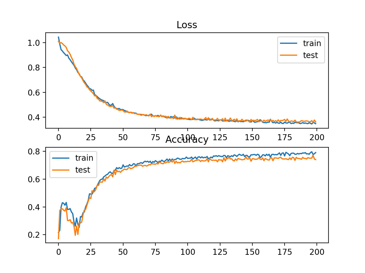
A figure is also created showing two line plots, the top with the cross-entropy loss over epochs for the train (blue) and test (orange) dataset, and the bottom plot showing classification accuracy over epochs.
The plot shows that the training process converged well. The plot for loss is smooth, given the continuous nature of the error between the probability distributions, whereas the line plot for accuracy shows bumps, given examples in the train and test set can ultimately only be predicted as correct or incorrect, providing less granular feedback on performance.
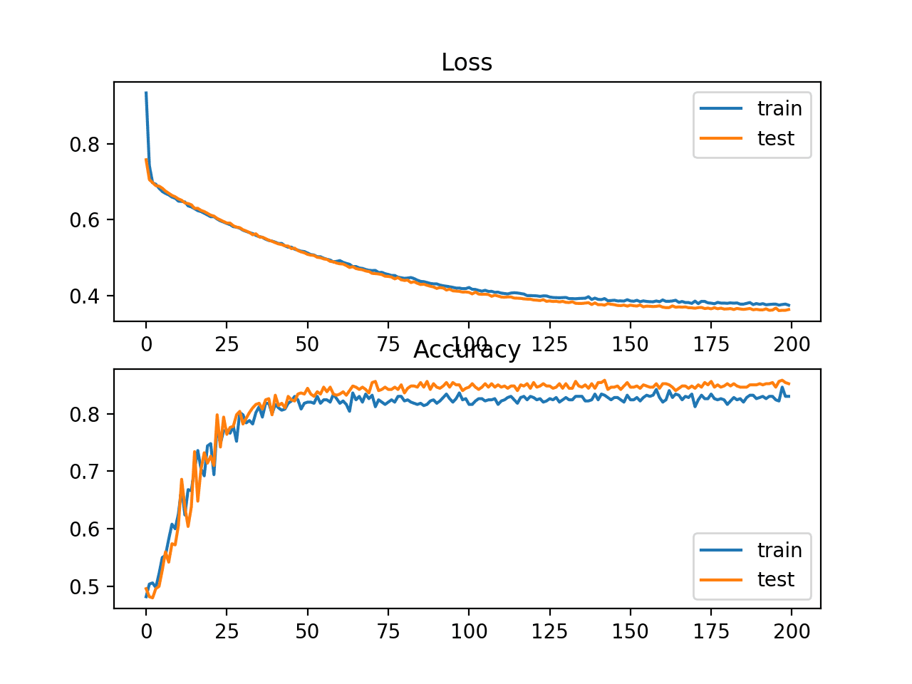
Line Plots of Cross Entropy Loss and Classification Accuracy over Training Epochs on the Two Circles Binary Classification Problem
Hinge Loss
An alternative to cross-entropy for binary classification problems is the hinge loss function, primarily developed for use with Support Vector Machine (SVM) models.
It is intended for use with binary classification where the target values are in the set {-1, 1}.
The hinge loss function encourages examples to have the correct sign, assigning more error when there is a difference in the sign between the actual and predicted class values.
Reports of performance with the hinge loss are mixed, sometimes resulting in better performance than cross-entropy on binary classification problems.
Firstly, the target variable must be modified to have values in the set {-1, 1}.
|
1 2 |
# change y from {0,1} to {-1,1} y[where(y == 0)] = -1 |
The hinge loss function can then be specified as the ‘hinge‘ in the compile function.
|
1 |
model.compile(loss='hinge', optimizer=opt, metrics=['accuracy']) |
Finally, the output layer of the network must be configured to have a single node with a hyperbolic tangent activation function capable of outputting a single value in the range [-1, 1].
|
1 |
model.add(Dense(1, activation='tanh')) |
The complete example of an MLP with a hinge loss function for the two circles binary classification problem is listed below.
|
1 2 3 4 5 6 7 8 9 10 11 12 13 14 15 16 17 18 19 20 21 22 23 24 25 26 27 28 29 30 31 32 33 34 35 36 37 38 39 40 |
# mlp for the circles problem with hinge loss from sklearn.datasets import make_circles from keras.models import Sequential from keras.layers import Dense from keras.optimizers import SGD from matplotlib import pyplot from numpy import where # generate 2d classification dataset X, y = make_circles(n_samples=1000, noise=0.1, random_state=1) # change y from {0,1} to {-1,1} y[where(y == 0)] = -1 # split into train and test n_train = 500 trainX, testX = X[:n_train, :], X[n_train:, :] trainy, testy = y[:n_train], y[n_train:] # define model model = Sequential() model.add(Dense(50, input_dim=2, activation='relu', kernel_initializer='he_uniform')) model.add(Dense(1, activation='tanh')) opt = SGD(lr=0.01, momentum=0.9) model.compile(loss='hinge', optimizer=opt, metrics=['accuracy']) # fit model history = model.fit(trainX, trainy, validation_data=(testX, testy), epochs=200, verbose=0) # evaluate the model _, train_acc = model.evaluate(trainX, trainy, verbose=0) _, test_acc = model.evaluate(testX, testy, verbose=0) print('Train: %.3f, Test: %.3f' % (train_acc, test_acc)) # plot loss during training pyplot.subplot(211) pyplot.title('Loss') pyplot.plot(history.history['loss'], label='train') pyplot.plot(history.history['val_loss'], label='test') pyplot.legend() # plot accuracy during training pyplot.subplot(212) pyplot.title('Accuracy') pyplot.plot(history.history['accuracy'], label='train') pyplot.plot(history.history['val_accuracy'], label='test') pyplot.legend() pyplot.show() |
Running the example first prints the classification accuracy for the model on the train and test dataset.
Note: Your results may vary given the stochastic nature of the algorithm or evaluation procedure, or differences in numerical precision. Consider running the example a few times and compare the average outcome.
In this case, we can see slightly worse performance than using cross-entropy, with the chosen model configuration with less than 80% accuracy on the train and test sets.
|
1 |
Train: 0.792, Test: 0.740 |
A figure is also created showing two line plots, the top with the hinge loss over epochs for the train (blue) and test (orange) dataset, and the bottom plot showing classification accuracy over epochs.
The plot of hinge loss shows that the model has converged and has reasonable loss on both datasets. The plot of classification accuracy also shows signs of convergence, albeit at a lower level of skill than may be desirable on this problem.
Line Plots of Hinge Loss and Classification Accuracy over Training Epochs on the Two Circles Binary Classification Problem
Squared Hinge Loss
The hinge loss function has many extensions, often the subject of investigation with SVM models.
A popular extension is called the squared hinge loss that simply calculates the square of the score hinge loss. It has the effect of smoothing the surface of the error function and making it numerically easier to work with.
If using a hinge loss does result in better performance on a given binary classification problem, is likely that a squared hinge loss may be appropriate.
As with using the hinge loss function, the target variable must be modified to have values in the set {-1, 1}.
|
1 2 |
# change y from {0,1} to {-1,1} y[where(y == 0)] = -1 |
The squared hinge loss can be specified as ‘squared_hinge‘ in the compile() function when defining the model.
|
1 |
model.compile(loss='squared_hinge', optimizer=opt, metrics=['accuracy']) |
And finally, the output layer must use a single node with a hyperbolic tangent activation function capable of outputting continuous values in the range [-1, 1].
|
1 |
model.add(Dense(1, activation='tanh')) |
The complete example of an MLP with the squared hinge loss function on the two circles binary classification problem is listed below.
|
1 2 3 4 5 6 7 8 9 10 11 12 13 14 15 16 17 18 19 20 21 22 23 24 25 26 27 28 29 30 31 32 33 34 35 36 37 38 39 40 |
# mlp for the circles problem with squared hinge loss from sklearn.datasets import make_circles from keras.models import Sequential from keras.layers import Dense from keras.optimizers import SGD from matplotlib import pyplot from numpy import where # generate 2d classification dataset X, y = make_circles(n_samples=1000, noise=0.1, random_state=1) # change y from {0,1} to {-1,1} y[where(y == 0)] = -1 # split into train and test n_train = 500 trainX, testX = X[:n_train, :], X[n_train:, :] trainy, testy = y[:n_train], y[n_train:] # define model model = Sequential() model.add(Dense(50, input_dim=2, activation='relu', kernel_initializer='he_uniform')) model.add(Dense(1, activation='tanh')) opt = SGD(lr=0.01, momentum=0.9) model.compile(loss='squared_hinge', optimizer=opt, metrics=['accuracy']) # fit model history = model.fit(trainX, trainy, validation_data=(testX, testy), epochs=200, verbose=0) # evaluate the model _, train_acc = model.evaluate(trainX, trainy, verbose=0) _, test_acc = model.evaluate(testX, testy, verbose=0) print('Train: %.3f, Test: %.3f' % (train_acc, test_acc)) # plot loss during training pyplot.subplot(211) pyplot.title('Loss') pyplot.plot(history.history['loss'], label='train') pyplot.plot(history.history['val_loss'], label='test') pyplot.legend() # plot accuracy during training pyplot.subplot(212) pyplot.title('Accuracy') pyplot.plot(history.history['accuracy'], label='train') pyplot.plot(history.history['val_accuracy'], label='test') pyplot.legend() pyplot.show() |
Running the example first prints the classification accuracy for the model on the train and test datasets.
Note: Your results may vary given the stochastic nature of the algorithm or evaluation procedure, or differences in numerical precision. Consider running the example a few times and compare the average outcome.
In this case, we can see that for this problem and the chosen model configuration, the hinge squared loss may not be appropriate, resulting in classification accuracy of less than 70% on the train and test sets.
|
1 |
Train: 0.682, Test: 0.646 |
A figure is also created showing two line plots, the top with the squared hinge loss over epochs for the train (blue) and test (orange) dataset, and the bottom plot showing classification accuracy over epochs.
The plot of loss shows that indeed, the model converged, but the shape of the error surface is not as smooth as other loss functions where small changes to the weights are causing large changes in loss.
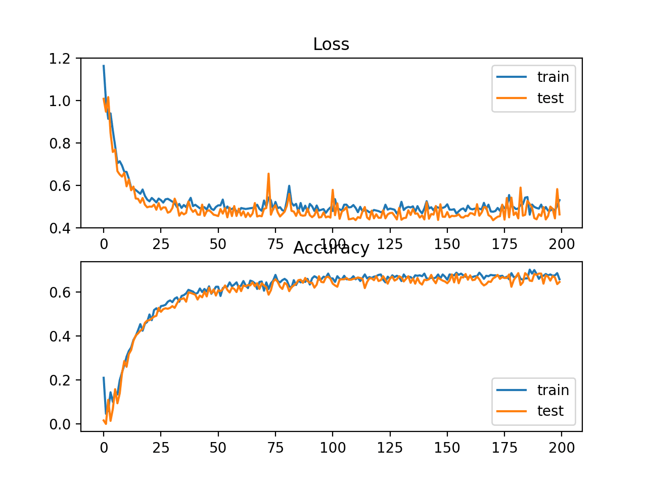
Line Plots of Squared Hinge Loss and Classification Accuracy over Training Epochs on the Two Circles Binary Classification Problem
Multi-Class Classification Loss Functions
Multi-Class classification are those predictive modeling problems where examples are assigned one of more than two classes.
The problem is often framed as predicting an integer value, where each class is assigned a unique integer value from 0 to (num_classes – 1). The problem is often implemented as predicting the probability of the example belonging to each known class.
In this section, we will investigate loss functions that are appropriate for multi-class classification predictive modeling problems.
We will use the blobs problem as the basis for the investigation. The make_blobs() function provided by the scikit-learn provides a way to generate examples given a specified number of classes and input features. We will use this function to generate 1,000 examples for a 3-class classification problem with 2 input variables. The pseudorandom number generator will be seeded consistently so that the same 1,000 examples are generated each time the code is run.
|
1 2 |
# generate dataset X, y = make_blobs(n_samples=1000, centers=3, n_features=2, cluster_std=2, random_state=2) |
The two input variables can be taken as x and y coordinates for points on a two-dimensional plane.
The example below creates a scatter plot of the entire dataset coloring points by their class membership.
|
1 2 3 4 5 6 7 8 9 10 11 |
# scatter plot of blobs dataset from sklearn.datasets import make_blobs from numpy import where from matplotlib import pyplot # generate dataset X, y = make_blobs(n_samples=1000, centers=3, n_features=2, cluster_std=2, random_state=2) # select indices of points with each class label for i in range(3): samples_ix = where(y == i) pyplot.scatter(X[samples_ix, 0], X[samples_ix, 1]) pyplot.show() |
Running the example creates a scatter plot showing the 1,000 examples in the dataset with examples belonging to the 0, 1, and 2 classes colors blue, orange, and green respectively.
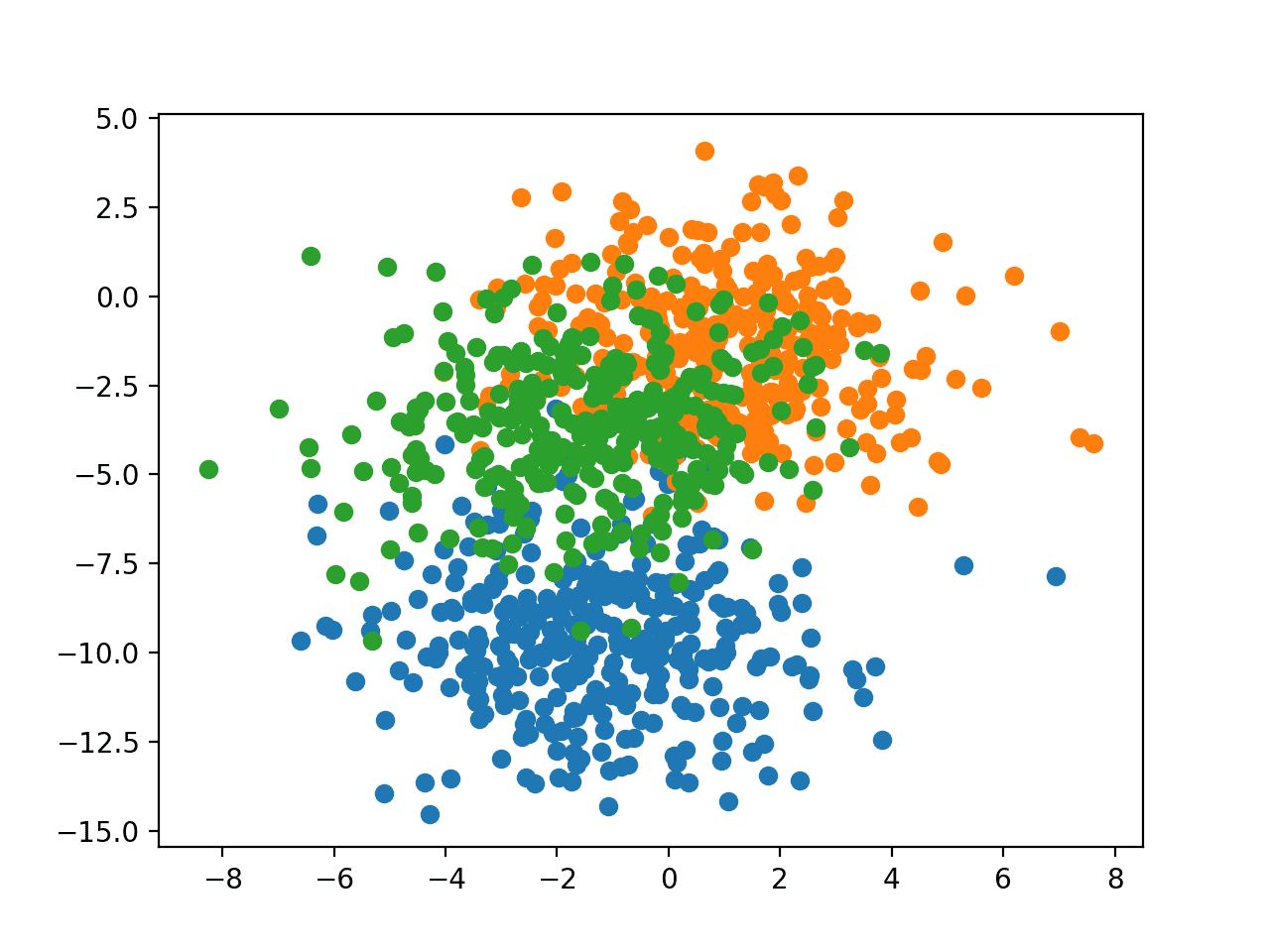
Scatter Plot of Examples Generated from the Blobs Multi-Class Classification Problem
The input features are Gaussian and could benefit from standardization; nevertheless, we will keep the values unscaled in this example for brevity.
The dataset will be split evenly between train and test sets.
|
1 2 3 4 |
# split into train and test n_train = 500 trainX, testX = X[:n_train, :], X[n_train:, :] trainy, testy = y[:n_train], y[n_train:] |
A small MLP model will be used as the basis for exploring loss functions.
The model expects two input variables, has 50 nodes in the hidden layer and the rectified linear activation function, and an output layer that must be customized based on the selection of the loss function.
|
1 2 3 4 |
# define model model = Sequential() model.add(Dense(50, input_dim=2, activation='relu', kernel_initializer='he_uniform')) model.add(Dense(..., activation='...')) |
The model is fit using stochastic gradient descent with a sensible default learning rate of 0.01 and a momentum of 0.9.
|
1 2 3 |
# compile model opt = SGD(lr=0.01, momentum=0.9) model.compile(loss='...', optimizer=opt, metrics=['accuracy']) |
The model will be fit for 100 epochs on the training dataset and the test dataset will be used as a validation dataset, allowing us to evaluate both loss and classification accuracy on the train and test sets at the end of each training epoch and draw learning curves.
|
1 2 |
# fit model history = model.fit(trainX, trainy, validation_data=(testX, testy), epochs=100, verbose=0) |
Now that we have the basis of a problem and model, we can take a look evaluating three common loss functions that are appropriate for a multi-class classification predictive modeling problem.
Although an MLP is used in these examples, the same loss functions can be used when training CNN and RNN models for multi-class classification.
Multi-Class Cross-Entropy Loss
Cross-entropy is the default loss function to use for multi-class classification problems.
In this case, it is intended for use with multi-class classification where the target values are in the set {0, 1, 3, …, n}, where each class is assigned a unique integer value.
Mathematically, it is the preferred loss function under the inference framework of maximum likelihood. It is the loss function to be evaluated first and only changed if you have a good reason.
Cross-entropy will calculate a score that summarizes the average difference between the actual and predicted probability distributions for all classes in the problem. The score is minimized and a perfect cross-entropy value is 0.
Cross-entropy can be specified as the loss function in Keras by specifying ‘categorical_crossentropy‘ when compiling the model.
|
1 |
model.compile(loss='categorical_crossentropy', optimizer=opt, metrics=['accuracy']) |
The function requires that the output layer is configured with an n nodes (one for each class), in this case three nodes, and a ‘softmax‘ activation in order to predict the probability for each class.
|
1 |
model.add(Dense(3, activation='softmax')) |
In turn, this means that the target variable must be one hot encoded.
This is to ensure that each example has an expected probability of 1.0 for the actual class value and an expected probability of 0.0 for all other class values. This can be achieved using the to_categorical() Keras function.
|
1 2 |
# one hot encode output variable y = to_categorical(y) |
The complete example of an MLP with cross-entropy loss for the multi-class blobs classification problem is listed below.
|
1 2 3 4 5 6 7 8 9 10 11 12 13 14 15 16 17 18 19 20 21 22 23 24 25 26 27 28 29 30 31 32 33 34 35 36 37 38 39 40 41 |
# mlp for the blobs multi-class classification problem with cross-entropy loss from sklearn.datasets import make_blobs from keras.layers import Dense from keras.models import Sequential from keras.optimizers import SGD from keras.utils import to_categorical from matplotlib import pyplot # generate 2d classification dataset X, y = make_blobs(n_samples=1000, centers=3, n_features=2, cluster_std=2, random_state=2) # one hot encode output variable y = to_categorical(y) # split into train and test n_train = 500 trainX, testX = X[:n_train, :], X[n_train:, :] trainy, testy = y[:n_train], y[n_train:] # define model model = Sequential() model.add(Dense(50, input_dim=2, activation='relu', kernel_initializer='he_uniform')) model.add(Dense(3, activation='softmax')) # compile model opt = SGD(lr=0.01, momentum=0.9) model.compile(loss='categorical_crossentropy', optimizer=opt, metrics=['accuracy']) # fit model history = model.fit(trainX, trainy, validation_data=(testX, testy), epochs=100, verbose=0) # evaluate the model _, train_acc = model.evaluate(trainX, trainy, verbose=0) _, test_acc = model.evaluate(testX, testy, verbose=0) print('Train: %.3f, Test: %.3f' % (train_acc, test_acc)) # plot loss during training pyplot.subplot(211) pyplot.title('Loss') pyplot.plot(history.history['loss'], label='train') pyplot.plot(history.history['val_loss'], label='test') pyplot.legend() # plot accuracy during training pyplot.subplot(212) pyplot.title('Accuracy') pyplot.plot(history.history['accuracy'], label='train') pyplot.plot(history.history['val_accuracy'], label='test') pyplot.legend() pyplot.show() |
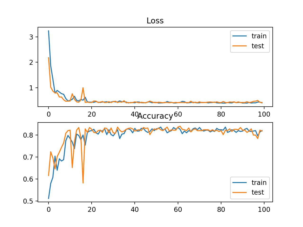
Running the example first prints the classification accuracy for the model on the train and test dataset.
Note: Your results may vary given the stochastic nature of the algorithm or evaluation procedure, or differences in numerical precision. Consider running the example a few times and compare the average outcome.
In this case, we can see the model performed well, achieving a classification accuracy of about 84% on the training dataset and about 82% on the test dataset.
|
1 |
Train: 0.840, Test: 0.822 |
A figure is also created showing two line plots, the top with the cross-entropy loss over epochs for the train (blue) and test (orange) dataset, and the bottom plot showing classification accuracy over epochs.
In this case, the plot shows the model seems to have converged. The line plots for both cross-entropy and accuracy both show good convergence behavior, although somewhat bumpy. The model may be well configured given no sign of over or under fitting. The learning rate or batch size may be tuned to even out the smoothness of the convergence in this case.
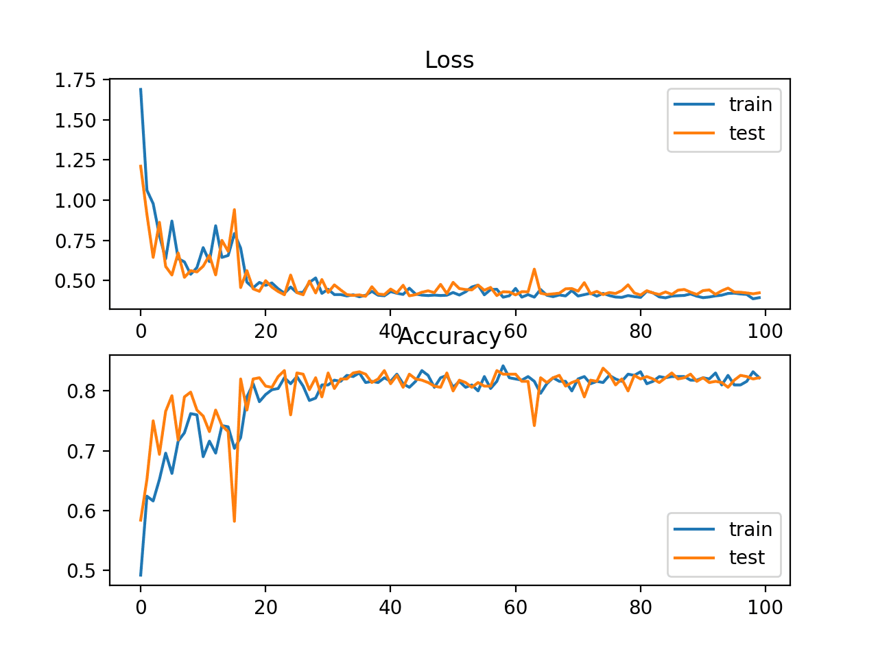
Line Plots of Cross Entropy Loss and Classification Accuracy over Training Epochs on the Blobs Multi-Class Classification Problem
Sparse Multiclass Cross-Entropy Loss
A possible cause of frustration when using cross-entropy with classification problems with a large number of labels is the one hot encoding process.
For example, predicting words in a vocabulary may have tens or hundreds of thousands of categories, one for each label. This can mean that the target element of each training example may require a one hot encoded vector with tens or hundreds of thousands of zero values, requiring significant memory.
Sparse cross-entropy addresses this by performing the same cross-entropy calculation of error, without requiring that the target variable be one hot encoded prior to training.
Sparse cross-entropy can be used in keras for multi-class classification by using ‘sparse_categorical_crossentropy‘ when calling the compile() function.
|
1 |
model.compile(loss='sparse_categorical_crossentropy', optimizer=opt, metrics=['accuracy']) |
The function requires that the output layer is configured with an n nodes (one for each class), in this case three nodes, and a ‘softmax‘ activation in order to predict the probability for each class.
|
1 |
model.add(Dense(3, activation='softmax')) |
No one hot encoding of the target variable is required, a benefit of this loss function.
The complete example of training an MLP with sparse cross-entropy on the blobs multi-class classification problem is listed below.
|
1 2 3 4 5 6 7 8 9 10 11 12 13 14 15 16 17 18 19 20 21 22 23 24 25 26 27 28 29 30 31 32 33 34 35 36 37 38 |
# mlp for the blobs multi-class classification problem with sparse cross-entropy loss from sklearn.datasets import make_blobs from keras.layers import Dense from keras.models import Sequential from keras.optimizers import SGD from matplotlib import pyplot # generate 2d classification dataset X, y = make_blobs(n_samples=1000, centers=3, n_features=2, cluster_std=2, random_state=2) # split into train and test n_train = 500 trainX, testX = X[:n_train, :], X[n_train:, :] trainy, testy = y[:n_train], y[n_train:] # define model model = Sequential() model.add(Dense(50, input_dim=2, activation='relu', kernel_initializer='he_uniform')) model.add(Dense(3, activation='softmax')) # compile model opt = SGD(lr=0.01, momentum=0.9) model.compile(loss='sparse_categorical_crossentropy', optimizer=opt, metrics=['accuracy']) # fit model history = model.fit(trainX, trainy, validation_data=(testX, testy), epochs=100, verbose=0) # evaluate the model _, train_acc = model.evaluate(trainX, trainy, verbose=0) _, test_acc = model.evaluate(testX, testy, verbose=0) print('Train: %.3f, Test: %.3f' % (train_acc, test_acc)) # plot loss during training pyplot.subplot(211) pyplot.title('Loss') pyplot.plot(history.history['loss'], label='train') pyplot.plot(history.history['val_loss'], label='test') pyplot.legend() # plot accuracy during training pyplot.subplot(212) pyplot.title('Accuracy') pyplot.plot(history.history['accuracy'], label='train') pyplot.plot(history.history['val_accuracy'], label='test') pyplot.legend() pyplot.show() |
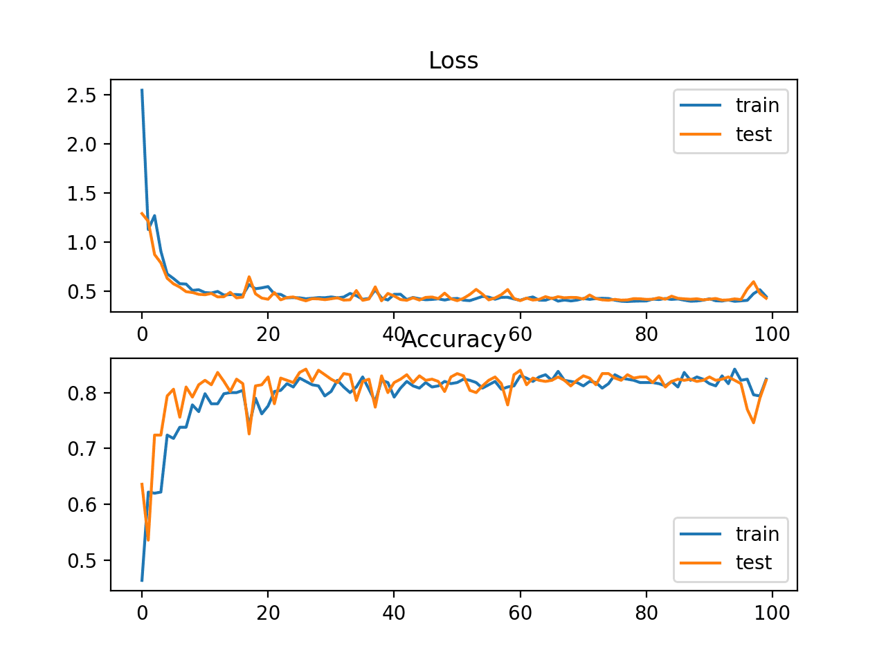
Running the example first prints the classification accuracy for the model on the train and test dataset.
Note: Your results may vary given the stochastic nature of the algorithm or evaluation procedure, or differences in numerical precision. Consider running the example a few times and compare the average outcome.
In this case, we can see the model achieves good performance on the problem. In fact, if you repeat the experiment many times, the average performance of sparse and non-sparse cross-entropy should be comparable.
|
1 |
Train: 0.832, Test: 0.818 |
A figure is also created showing two line plots, the top with the sparse cross-entropy loss over epochs for the train (blue) and test (orange) dataset, and the bottom plot showing classification accuracy over epochs.
In this case, the plot shows good convergence of the model over training with regard to loss and classification accuracy.
Line Plots of Sparse Cross Entropy Loss and Classification Accuracy over Training Epochs on the Blobs Multi-Class Classification Problem
Kullback Leibler Divergence Loss
Kullback Leibler Divergence, or KL Divergence for short, is a measure of how one probability distribution differs from a baseline distribution.
A KL divergence loss of 0 suggests the distributions are identical. In practice, the behavior of KL Divergence is very similar to cross-entropy. It calculates how much information is lost (in terms of bits) if the predicted probability distribution is used to approximate the desired target probability distribution.
As such, the KL divergence loss function is more commonly used when using models that learn to approximate a more complex function than simply multi-class classification, such as in the case of an autoencoder used for learning a dense feature representation under a model that must reconstruct the original input. In this case, KL divergence loss would be preferred. Nevertheless, it can be used for multi-class classification, in which case it is functionally equivalent to multi-class cross-entropy.
KL divergence loss can be used in Keras by specifying ‘kullback_leibler_divergence‘ in the compile() function.
|
1 |
model.compile(loss='kullback_leibler_divergence', optimizer=opt, metrics=['accuracy']) |
As with cross-entropy, the output layer is configured with an n nodes (one for each class), in this case three nodes, and a ‘softmax‘ activation in order to predict the probability for each class.
Also, as with categorical cross-entropy, we must one hot encode the target variable to have an expected probability of 1.0 for the class value and 0.0 for all other class values.
|
1 2 |
# one hot encode output variable y = to_categorical(y) |
The complete example of training an MLP with KL divergence loss for the blobs multi-class classification problem is listed below.
|
1 2 3 4 5 6 7 8 9 10 11 12 13 14 15 16 17 18 19 20 21 22 23 24 25 26 27 28 29 30 31 32 33 34 35 36 37 38 39 40 41 |
# mlp for the blobs multi-class classification problem with kl divergence loss from sklearn.datasets import make_blobs from keras.layers import Dense from keras.models import Sequential from keras.optimizers import SGD from keras.utils import to_categorical from matplotlib import pyplot # generate 2d classification dataset X, y = make_blobs(n_samples=1000, centers=3, n_features=2, cluster_std=2, random_state=2) # one hot encode output variable y = to_categorical(y) # split into train and test n_train = 500 trainX, testX = X[:n_train, :], X[n_train:, :] trainy, testy = y[:n_train], y[n_train:] # define model model = Sequential() model.add(Dense(50, input_dim=2, activation='relu', kernel_initializer='he_uniform')) model.add(Dense(3, activation='softmax')) # compile model opt = SGD(lr=0.01, momentum=0.9) model.compile(loss='kullback_leibler_divergence', optimizer=opt, metrics=['accuracy']) # fit model history = model.fit(trainX, trainy, validation_data=(testX, testy), epochs=100, verbose=0) # evaluate the model _, train_acc = model.evaluate(trainX, trainy, verbose=0) _, test_acc = model.evaluate(testX, testy, verbose=0) print('Train: %.3f, Test: %.3f' % (train_acc, test_acc)) # plot loss during training pyplot.subplot(211) pyplot.title('Loss') pyplot.plot(history.history['loss'], label='train') pyplot.plot(history.history['val_loss'], label='test') pyplot.legend() # plot accuracy during training pyplot.subplot(212) pyplot.title('Accuracy') pyplot.plot(history.history['accuracy'], label='train') pyplot.plot(history.history['val_accuracy'], label='test') pyplot.legend() pyplot.show() |
Running the example first prints the classification accuracy for the model on the train and test dataset.
Note: Your results may vary given the stochastic nature of the algorithm or evaluation procedure, or differences in numerical precision. Consider running the example a few times and compare the average outcome.
In this case, we see performance that is similar to those results seen with cross-entropy loss, in this case about 82% accuracy on the train and test dataset.
|
1 |
Train: 0.822, Test: 0.822 |
A figure is also created showing two line plots, the top with the KL divergence loss over epochs for the train (blue) and test (orange) dataset, and the bottom plot showing classification accuracy over epochs.
In this case, the plot shows good convergence behavior for both loss and classification accuracy. It is very likely that an evaluation of cross-entropy would result in nearly identical behavior given the similarities in the measure.
Line Plots of KL Divergence Loss and Classification Accuracy over Training Epochs on the Blobs Multi-Class Classification Problem
Further Reading
This section provides more resources on the topic if you are looking to go deeper.
Posts
Papers
API
- Keras Loss Functions API
- Keras Activation Functions API
- sklearn.preprocessing.StandardScaler API
- sklearn.datasets.make_regression API
- sklearn.datasets.make_circles API
- sklearn.datasets.make_blobs API
Articles
- Mean squared error, Wikipedia.
- Mean absolute error, Wikipedia.
- Cross entropy, Wikipedia.
- Hinge loss, Wikipedia.
- Kullback–Leibler divergence, Wikipedia.
- Loss Functions in Neural Networks, 2017.
Summary
In this tutorial, you discovered how to choose a loss function for your deep learning neural network for a given predictive modeling problem.
Specifically, you learned:
- How to configure a model for mean squared error and variants for regression problems.
- How to configure a model for cross-entropy and hinge loss functions for binary classification.
- How to configure a model for cross-entropy and KL divergence loss functions for multi-class classification.
Do you have any questions?
Ask your questions in the comments below and I will do my best to answer.
Develop Better Deep Learning Models Today!

Train Faster, Reduce Overftting, and Ensembles
...with just a few lines of python code
Discover how in my new Ebook:
Better Deep Learning
It provides self-study tutorials on topics like:
weight decay, batch normalization, dropout, model stacking and much more...
Bring better deep learning to your projects!
Skip the Academics. Just Results.


That was a very good tutorial about loss functions, found your blog some time ago, but read this article today. Will read more articles for sure!
Antonius Kasbergen
Thanks, I’m glad it helped Antonius!
Avid follower of your ever reliable blogs Jason.
I need your advise for a regression problem that have input features with different probability distribution. Do we need to scale them differently? lastly, is it advisable to scale the target variable as well?
Thanks
Dennis
Perhaps. It really depends on the data.
Often it is a good idea to scale the target variable as well.
I noticed that you apply the StandardScaler to both the feature data, and the response variable data. Throughout your website there are many examples where you do not scale the response variable data. Why did you do that in this example.
It is a good practice for regression. I often leave it out for brevity as the focus of the tutorial is something else.
hello Jason Brownlee,
i really thanks for your blog to make me learn lots of AI . can you help me ?
with binary cross_entropy task, can i make the output layer of Dense with 2 nodes not 1 like below ?
model.add(Dense(2, activation=’sigmoid’))
Why have 2 nodes in the output with sigmoid activation?
i want to get each probability of value 1 ,value 0.
Yes. What is the problem exactly?
@sanjie I think you just need one, since the probability of the other will be 1 minus the one you get. Example: you get probability of 0.63 of being 1, then the prob. of being 0 is 1-0.63 = 0.27. Otherwise you can end the net with 2 neurons and softmax. This last strategy extends to any number.
Hi,
I’ve been reading this post and the other one of ‘How to use metrics for DL’, and it rose a doubt. Apparently we can create custom metrics but we can not create custom loss functions in keras. Or am I wrong?
I understand a custom loss function would need its gradients to perform backpropagation, but do you know if we can do so in Keras?
Thanks
You can create custom loss functions, but really need to know what you’re doing.
Hi Dr. Brownlee,
I have a very demanding dataset, and I’m doing binary classification on this dataset. Instead of using the keras imports, I used “tf.keras” from the new TensorFlow 2.0 alpha. When I copied your plotting code to show the “loss” and “val_loss” I got a very interesting charts. I’d like to show these charts. How can I include a chart on this reply group?
Charles:
Perhaps you can post your charts on your own website, blog, image hosting site, or github and link to them?
I put my notebook on GitHub. Please look at:
https://github.com/CBrauer/CypressPoint.github.io/blob/master/rocket.ipynb
Any comments will be greatly appreciated.
Charles
From the plot of loss, it looks like you are overfitting.
See this post:
https://machinelearningmastery.com/learning-curves-for-diagnosing-machine-learning-model-performance/
How is Mean absolute error loss robust to outliers?
Error outliers, not outliers in the data.
It seems to me that MAE would be treating type1 and type2 errors are the same error.
So I may not call that ‘robust to model errors’ – but perhaps the use case here is when type1 and type2 have the same cost to business, and one is not more impactful than the other.
Thanks for sharing.
How can I define a new loss function in which the error is computed based on the mean of all predicted values, i.e., loss = y_pred – mean(y_pred)?
You can define a loss function to do anything you wish.
To calculate the mean of a tensor use the Keras backend:
from keras import backend as K
…
K.mean(…)
Hi Jason,
Thanks for the great blog.
I wanted to know whether we must only use binary cross entropy for autoencoder training? and if we go with binary cross entropy, should we transform the input to be between (0,1) ?
If you are working with a binary sequence, then binary cross entropy may be more appropriate.
Hi Jason,
Great tutorial!
By looking at the loss plots I can see some similarities with my own experience. But this has allways bugged me a bit: should the loss plateaus like you showed for MSE? I’m asking because I saw this behaviour on my own problems and I worried it could be a bad minima.
This post will help in interpreting plots of loss:
https://machinelearningmastery.com/learning-curves-for-diagnosing-machine-learning-model-performance/
First of all, I am really grateful for your effort. When I look for a solution about deep learning, your blog is always the right one. thanks a lot.
My question is about binary classification loss function.
I have a binary output, and I coded output value as either -1 or 1, as you mention in hinge loss function.
Also, input variables are either categorical (multi-class) or binary . I coded binary variables as 0 or 1, and coded categorical variable with Label Binarizer. I am using Conv1D networks.
Should I change encoding of input variables to make it similar with output format? I mean at the end, should input variables be either -1 or 1, instead of 0 or 1, to perform Hinge loss function?
Thanks in advance
Thanks!
Hinge loss is only concerned with the output of the model, e.g. outputs must be in [-1,1] and you should use the tanh activation function.
You can have inputs in any form you wish, although normalization or standardization is a good idea generally.
Jason, I think there is a mistake in your writing. Search this web page for logistic. It will show up in 2 places. I think you meant to say logarithmic … right?
Thanks.
Updated for consistency.
Hi Jason,
Just wanted to confirm my understanding because I’m still pretty new to neural networks and Keras. Since MLP needs to have at least 3 layers (input, hidden, and output layer), does input_dim=20 your input layer?
Thank you!
An MLP could have 1 layer, there are no rules.
input_dim always defines the number of inputs in a given input sample.
“a perfect cross-entropy value is 0.”
Wouldn’t a “perfect” cross-entropy value be equal to the entropy of the true distribution, rather than zero? And perhaps that’s why the loss in your graph seems to be converging to ~0.4?
No, cross entropy calculates the difference between two distributions.
More precisely, the average total bits to encode an event from one distribution compared to the other distribution.
We never hit zero in practice, unless we overfit like crazy or the problem is trivial.
where does val_loss comes from? I’m getting error ‘KeyError: ‘val_loss”
It comes from the history, but it assumes you are using a validation dataset when fitting your model.
Hi Jason,
I have a regression problem where I have 7 input variables and want to use these to estimate two output variables. These two variables range from 0 to 1 but are distinct and depend on the 7 variables combined. Do I have to train two different models or can this be done with just one model?
Thanks
Sounds like you could model it as a multi-output regression problem and try a MSE loss as a first step?
Thanks Jason, although, I have not really found how to do a multi-output regression. Is it just a matter of having the last layer in your network be a Dense layer as below:
model.add(Dense(2))
model.compile(loss=’mean_squared_error’, optimizer=’Adam’)
Thanks again.
Correct!
Hi Jason,
I have collected the data for my multi output regression problem. I can see a possible issue here as the histogram of the output that I am trying to predict looks like a multi-peak (camels back) curve with about 4 peaks and a very wide range of values in the bin count (min 35 to max 5000). I have now finalized 9 input variables and 2 output variables. (Both the output variables have distribution as described before).
In a regression problem, is there such a thing as data augmentation? Should I be augmenting the data as whatever I do to the data will not reflect reality as I am trying model a physical dynamic system?
There is, but perhaps start with a simple supervised learning model as a first step and get something working.
I am doing as my first neural net problem a regression analysis with 1 input, but 8 outputs. I’m doing a fit to a power series of the x input, and trying to learn the first 8 coefficients of a power series expansion. I want to use a MSE loss function, but how do I tell the model what functional form I’m looking for? I really want to be able to print out the learned coefficients in the output layer.
Good question.
The trick of neural nets is you don’t tell it the function. You either don’t know the function, or in your case, you pretend you don’t know it, then you let the network learn the function from the inputs and outputs alone.
Does that help?
I think I found it in the keras documentation. I have to customize a loss function, and that’s where I input the power series functionality. It’s kind of cool- some number of output coefficients, and I can optimize the coefficients to get a random best fit. I could do it analytically, but it’s kind of a pain manually. When one has tons of data, it sounds easy!
Happy to hear that. Let me know how you go.
Hi Jason,
I need to implement a custom loss function of the following sort:
average_over_all_samples_in_batch( sum_over_k( x_true-x(k) ) )
where k is the index of the hidden layers. Therefore, x(k) refers to one of the outputs at hidden layer k. Of course this is a simplified version of my actual loss function, just enough to capture the essence of my question. To give some context, my neural network is sort of like a recursive detection network.
I implement my model using the tensorflow functional API, with some custom layers, all wrapped into a model, which I then train with methods like model.compile, model.fit,… etc
Could you suggest how I can go about implementing the custom loss function? Or is there any resource I could refer to? I haven’t been able to find any clear ones.
Not off hand sorry, I think you will have to do some experimentation to see if it is feasible.
Hi Jason
I implemented an Auto-encoder algorithm for anomaly detection in network dataset, but my loss value was still high and the accuracy was 68% which is not too good. Do you have an Auto-encoder code that will help to clear me well on that area, because I am still a beginner in the field of ML and DL. Also, I am having problem in writing code for visualization of the model outcome. Thanks for tutoring. I am really enjoying your tutorials.
Sorry, I don’t have many autoencoder examples.
These tutorials may help you improve performance:
https://machinelearningmastery.com/start-here/#better
Hi Jason. I’ very new to deep learning and your blogs are really helpful.
I wanted to know why do we use [:,0] here-
y = StandardScaler().fit_transform(y.reshape(len(y),1))[:,0]
To get the first column.
More on array indexes and slices:
https://machinelearningmastery.com/index-slice-reshape-numpy-arrays-machine-learning-python/
How can I cite your articles in my research works
Good question, see this:
https://machinelearningmastery.com/faq/single-faq/how-do-i-reference-or-cite-a-book-or-blog-post
It was crisp, to the point and clearly understandable to apply the concept of Losses
Thanks!
Hi Jason,
Thanks for awesome tutorial.
What should we use for multi-label classification (where 1 or more classes can be assigned to an input) ?
Also, I think, it would be nice if you can add mathematical formulas (or python codes with numpy) of each loss function.
Binary cross entropy loss.
Thanks for the suggestion.
Hi,
I have a question regarding using the mse loss function for an image to image type of regression problem, however my training data are 4x the resolution than the label data. When trying to train the model, the code crashes while using MSE because the target and output have different shapes. What to do?
Thanks,
Yochanan
Perhaps try different models? different data preparation? different loss? etc.
never mind again, thanks
No problem.
Hi Jason, do you have a tutorial on implementing custom loss functions in Keras ?
Thanks
I have an example of a custom metric that could be used as a loss function:
https://machinelearningmastery.com/custom-metrics-deep-learning-keras-python/
Hello Jason,
Thanks for your article. I have a question. Is it possible to return a float value instead of a tensor in loss function? for example let’s say I have three NN and a global variable score(mean of y_pred of NN3). I want NN1 to return score value, NN2 to return (score*-1) and NN3 loss would be (NN1 Loss – NN2 Loss). I have coded this way but I am almost certain that it’s not working.
def NN1Loss():
def loss(y_true, y_pred):
global N1_loss, score
score = tf.cast(score, “float32”)
return score + K.mean(y_true-y_pred)*0
return loss
This tutorial will show you how to create a custom metric that you can adapt to be a loss function:
https://machinelearningmastery.com/custom-metrics-deep-learning-keras-python/
Hi Jason,
Regarding the first loss plot (Line plot of Mean Squared Error Loss over Training Epochs When Optimizing the Mean Squared Error Loss Function) It seems that the ~30th epoch up to the 100th epoch are not needed (since the loss is already infintly small).
Is there a reason you still chose to pass the dataset through the neural network 100 times?
Thank you
Yes, to have all of the examples consistent.
We are demonstrating loss functions in this tutorial, not trying to get the best model or training scheme.
got it, thank you.
However, I encountered a case where my model’s (linear regression) predictions were good only for about 100 epochs, wereas the loss plot reached ~zero very fast (say at the 10th epoch).
Are you familiar with any reason that may cause this phenomenon?
(When I decreased the number of epochs, because they are seemingly unnecessary, the model’s perdications were much less good).
Thank you!
Perhaps explore learning curves for your model:
https://machinelearningmastery.com/learning-curves-for-diagnosing-machine-learning-model-performance/
Hi Jason,
Thanks for this great tutorial! Can Sparse Multiclass Cross-Entropy Loss be used for a 2-class classification problem? Thanks!
Perhaps, but why not use binary cross entropy and model the binomial distribution directly?
Off topic.
There is the question of how to provide artificial neural with large amounts of external memory they can actually use. Maybe If-Except-If trees can provide an answer.
https://discourse.numenta.org/t/numenta-research-meeting-july-27/7760/3
If neural networks can tolerate crossing the neural/symbolic barrier a couple of times then I think they should be able to learn how to use If-Except-If trees as a form of associative memory.
https://github.com/S6Regen/If-Except-If-Tree
Thanks for sharing.
Hi Jason,
Thanks for the article. I noticed that when I used L2/MSE loss for training an LSTM in PyTorch, it converged rather quickly. On the other hand, when I used L1/MAE loss, the network converged in about the same number of epochs, but after one more epoch it just output incredibly small values – almost like a line. MSE suffered from no such issue, even after training for 2x the epochs as MAE.
Do you think MAE would be more prone to overfitting than MSE when RNNs are concerned? Or is the “straight line/small range output” due to some other reason?
Regards
Tough question. I think it really depends on the specific dataset and model, e.g. these elements and the loss function all interact.
Hi Jason,
I have no problem with hinge loss for classification. but, I have a strange result when I used L1 cross-entropy loss function( y.log(yhat)-(1-y)log(1-yhat)), I got this error: RuntimeWarning: invalid value encountered in log.
I know this has happened because a negative number, I don’t how to avoid negative number?
I take absolute value of yhat but loss graph look wired (negative loss values under zero).
Targets must be 0 or 1 (binary) when using cross entropy loss.
Can we use Earth movers distance as loss function in auto encoders?
Perhaps, maybe try it and compare results to simple reconstruction error.
Hi Jason,
Is there any “max absolute error” for LSTM optimizer loss? I want to forecast time series and
need max absolute error. If there is none, how I can manually do it?
Thanks in advance
What is max absolute error?
hi jason,
i get the following error when i tried to test the code of “regression with mae loss function”.
i used Googlecolab to test your code.
Train: 0.002, Test: 0.002
—————————————————————————
KeyError Traceback (most recent call last)
in ()
—-> 1 import MLP_regre
/content/drive/My Drive/GooCo_app/MLP_regre.py in ()
36 pyplot.subplot(212)
37 pyplot.title(‘Mean Squared Error’)
—> 38 pyplot.plot(history.history[‘mean_squared_error’], label=’train’)
39 pyplot.plot(history.history[‘val_mean_squared_error’], label=’test’)
40 pyplot.legend()
KeyError: ‘mean_squared_error’
Sorry to hear that, these tips may help:
https://machinelearningmastery.com/faq/single-faq/why-does-the-code-in-the-tutorial-not-work-for-me
I was facing the same issue, I read about it in the documentation.
I could resolve this by using “mse” instead of “mean_squared_error”, and “val_mse” instead of “val_mean_squared_error”
Well done.
Can mean absolute error loss function be used for MLP classfier? IF not, what are the best loss functions for MLP classifier?
Yes, if you like.
The best loss function is the one that is a close fit for the metric you want to optimize for your project.
Hi Jason,
Thank you for the great tutorial. I have a question regarding multi-class classification.
As you said, “The problem is often framed as predicting an integer value…”. However, what would you suggest if we had classes for which we have to include custom loss in PyTorch regarding the content and order in these classes (original values)?
For example, let’s say we have classes ‘A1B1’, ‘A2B1’, ‘A2B2’, ‘A1B2’. So, I need to implement a custom loss (at least as a (learnable) regularization of cross-entropy loss). For simplicity, that can be some distance between class-elements.
thank you
Cross entropy is exactly this.
Hi Jason,
Thank you. Pardon me if I’m wrong. I understand that cross-entropy calculates the difference between two distributions (between input classes and output classes). However, I would need to catch the impact of class elements and ‘punish’ the network to correct the ‘whole’ class’s distribution if some part is misclassified. For example, if input data is ‘A1B1’ and predicted is ‘A2B1’ I have to create some custom class cross-entropy loss with the impact of misclassifying the first part of the class. The problem has classes with more parts – I have simplified it here to two parts just to have a simple demo.
I would appreciate any advice or correction in my reasoning
thank you
Why not treat them as mutually exclusive classes and punish all miss classifications equally?
You can develop a custom penalty for near misses if you like and add it to the cross entropy loss.
Hi Jason,
Thank you.
“Why not treat them as mutually exclusive classes and punish all miss classifications equally?”
• I did not quite understand what do you mean by “treat them”. Could you be so kind as to give more instructions? I would punish them differently since there is a difference (in significance) if the network misclassified the first or some other part.
“You can develop a custom penalty for near misses if you like and add it to the cross-entropy loss.”
• Do you have some examples on your site or in some of your books for that?
thank you
I meant: model the problem as though the classes are mutually exclusive.
I may have some exampels of custom loss functions on the blog, perhaps you can adapt the example here:
https://machinelearningmastery.com/custom-metrics-deep-learning-keras-python/
Is the code for evaluating the above one using confusion matrix and other parameters available. Also, does the train and test accuracy have to be the same for a good model?
If you need help with the confusion matrix, you can start here:
https://machinelearningmastery.com/confusion-matrix-machine-learning/
Thanka a lot!!! .I love this site so much. So helpful for a novice.
You’re welcome.
THX so much for this highly valuable blog !
If I may, I have a question on loss functions : I build a Conv1D model in to classify items into 6 categories (from 0 to 5).
I use therefore CrossEntropy Loss function that penalizes the errors with high probabilities but also the low probabilities associated to right answers. And that is what I was looking for.
But CrossEntropy considers the classes as independent, while I’d like reduce the loss for an error between two classes nearby and increase the loss for distant classes : i.e; reduce the loss where model predicts 0 (cat) while it is 1 (dog) and increase the loss when the model predicts 0 (cat) when the true answer is class 5 (fish).
Is there a way to embed the class proximity in the loss computation of a classification problem ? Thanks in advance for any help !
You’re welcome.
Perhaps try mean squared error loss?
Hi Jason,
I appreciate this concise tutorial about loss functions options on machine learning!
From time to time, its is very useful, after been working with many MLP, CNN, LSTM nets, stopping and sum up on the impact and implementation options of all the loss function used on our ML algorithms!
Very reflexive!
Thank you!
Hi Jason, thank you very much for this blog I use it allot!!!
I have a question about loss functions, maybe you could help.
I am building a model that outputs three values that sums up to 100(%) (somthing in soil science called texture). In past literture thay measured model successes based on R-square values to a 1:1 line and RMSE, for every output by itself (3 in total). Those two values (R-square and RMSE) are really affected by the total range of the test set (max-min) so it is hard to evluate model successes.
My question is if you know a loss function that takes into consideration the range of values in the training and test set?
thnks!!
You’re welcome.
Sounds like a multi-class classification, you can evaluate with cross-entropy, not RMSE or R^2. Cross entropy loss would also be appropriate, e.g. categorical cross entropy.
Values for the classes in the training set must have the same range, e.g. 0-1 for each label.
Hi jason
and thanks for this blog , I learned a lot .
A question about the choice of the loss function :
does this have an impact when used with an EarlyStopping callback.
If so , ca you give me an example or a list :
For example : if I use kullback_leibler_divergence should I apply a callback like this EarlyStopping(monitor=’val_loss’, patience=15)
or should I used another value to monitor ?
You’re welcome.
Loss defines the problem. Early stopping only helps to reduce overfitting/improve generalization of the model – it does not care what loss you use.
Hello jason,
Thank you for this nice tutorial.
I have studied that model is trained using the loss function. Then what is the role of cost function on model development?
Also i have studied that weight get update using the loss function they we nee to define cost function
Loss and cost function are the same thing.
Greate blog, custom loss functions would be a welcome blog if you have time
Thanks for the suggestion!
Hi Jason!
I am writing to you after around 2 years. Back then I learnt alot from your machine learning articles. Now I am again reading your articles on deep learning! Thank you so much for providing so much wonderful explanations. It means a lot! Please do keep writing more blogs
Thank you.
Hey Jason,
What type of loss function would you recommend if the distribution of the target is a strong bimodal distribution?
Thank you for all the wonderful blog posts. They have been a major help in my development of neural networks.
Hi Brendan…The following may help clarify:
https://towardsdatascience.com/anchors-and-multi-bin-loss-for-multi-modal-target-regression-647ea1974617
Hey Jason,
thanks for the amazing tutorial.
I’m trying to design a deep neural network where the model has to read a bunch of xls files and target prediction is between 3 classes (1, 2 and 3)
I’ve tried to use all the loss functions mentioned above but none of the loss functions are able to improve the ‘accuracy’. Which loss function would ou suggest?
Hi Yas…You may want to consider optimization techniques and/or feature selection to improve accuracy:
https://machinelearningmastery.com/feature-selection-to-improve-accuracy-and-decrease-training-time/
https://machinelearningmastery.com/machine-learning-performance-improvement-cheat-sheet/
Hi James,
So the aim of my task is to ‘train a Classifier’ without using Feature Selection. I now have a bigger data set(1400 csv files) and still get an accuracy of around 32%.
I’ve heard using some filter on the data set before using it to train the model might help. Do you have any tutorials on that?
Or any other suggestion for me?
Thanks!
Great article! Am using it heavily for revision.
Quick question: In MSLE I notice you say that in two example graphs, one shows signs of overfitting because the error starts to rise again as epochs progress.
How is it that both lines are rising if it’s overfitting? Shouldn’t the train line continue to fall but the test line rise, to show that the model is now fitting itself to the training data at the expense of being able to generalise?
Hi Bernie…the following resource may help clarify:
https://machinelearningmastery.com/introduction-to-regularization-to-reduce-overfitting-and-improve-generalization-error/
Hi,
I’m currently writing my bachelor thesis, I’m in the research phase and I need help!
I learned how to train a network for binary classification, but in my theory it’s a multiclass classification with more than 100 classes (snake type detection).
The activation of the output function I learned was sigmoid,
now I’m confused as to which loss/activation function i should use! how can i turn the output of the last layer with an activation function to a probabiliy for over a 1000 classes!
should i use for multi class!
I appreciate any help!
Hi Abed…You may find the following of interest:
https://machinelearningmastery.com/choose-an-activation-function-for-deep-learning/
Hi Jason, I thought I left a comment but it doesn’t appear here so I am leaving it again. I apologize if it’s duplicated. I’m really excited and glad that I found this article because I have been looking for how to implement hinge loss for binary classification and could not find clear guidance. I’m trying to explore the ensemble technique in semantic segmentation model (Unet/resnet/deeplab+SVM) and will compare to the single model use. I found that I can use hinge loss and it works same as SVM so I wanted to try this. I have 2 questions actually one is
1. do you think it will also work for semantic segmentation tasks? It’s the same logic so in theory, it should work the same but I am not confident of this since I’m a pretty beginner in computer vision.
2. if I can implement this to semantic models. Should I use tanh activation function for every layer of the model? or only for the last layer? Thank you very much in advance!
Hi dspeanut…the following may be of interest to you:
https://www.jeremyjordan.me/semantic-segmentation/
Question: When decide a factor (number of the factor) in the financial situation, like the factor in the stock market. And I use deep learning to get the W, the W it is the gradient decent number, like the slope in the regression. Will this W is my factor?
In the f(xi, W, b) = Wxi + b, the multiple dimension situation. And if W could be the detailed number of the factor? (factor is used in the financial situation, such as the factor of the stocks..) I’m not very sure..
Hi Helena…The following resource may be of interest:
https://wandb.ai/site/articles/fundamentals-of-neural-networks
Really appreciate your tutorial!!
A comprehensive article from different angles. i think the article may give the answer, and i should also process the biased data.
Hi Jason, I have a unet model and I’m trying to train it to do image segmentation but my loss I get is negative and low accuracy. I thought probably the loss function I’m using is wrong which is Binary cross-entropy, what other loss functions do you suggest?
Hi Sara…You may find the following resource of interest:
https://dev.to/_aadidev/3-common-loss-functions-for-image-segmentation-545o
Hi Jason,
When we train a multi-modal network for multi-class classification like document image classification (10-15 classes) using OCR text (BERT) and document image (VGG16) with early fusion, which loss function is ideal?
Hi Mujeeb…The following resource may be of interest to you:
https://towardsdatascience.com/handwriting-to-text-conversion-using-time-distributed-cnn-and-lstm-with-ctc-loss-function-a784dccc8ec3