How to Use Metrics for Deep Learning with Keras in Python

By Jason Brownlee on August 9, 2017 in Deep Learning

Last Updated on August 27, 2020

The Keras library provides a way to calculate and report on a suite of standard metrics when training deep learning models.

In addition to offering standard metrics for classification and regression problems, Keras also allows you to define and report on your own custom metrics when training deep learning models. This is particularly useful if you want to keep track of a performance measure that better captures the skill of your model during training.

In this tutorial, you will discover how to use the built-in metrics and how to define and use your own metrics when training deep learning models in Keras.

After completing this tutorial, you will know:

How Keras metrics work and how you can use them when training your models.
How to use regression and classification metrics in Keras with worked examples.
How to define and use your own custom metric in Keras with a worked example.

Kick-start your project with my new book Deep Learning With Python, including step-by-step tutorials and the Python source code files for all examples.

Let’s get started.

Update Jan/2020: Updated API for Keras 2.3 and TensorFlow 2.0.

Metrics and How to Use Custom Metrics for Deep Learning with Keras in Python
Photo by Indi Samarajiva, some rights reserved.

Tutorial Overview

This tutorial is divided into 4 parts; they are:

Keras Metrics
Keras Regression Metrics
Keras Classification Metrics
Custom Metrics in Keras

Keras Metrics

Keras allows you to list the metrics to monitor during the training of your model.

You can do this by specifying the “metrics” argument and providing a list of function names (or function name aliases) to the compile() function on your model.

For example:

model.compile(..., metrics=['mse'])

1	model.compile(..., metrics=['mse'])

The specific metrics that you list can be the names of Keras functions (like mean_squared_error) or string aliases for those functions (like ‘mse‘).

Metric values are recorded at the end of each epoch on the training dataset. If a validation dataset is also provided, then the metric recorded is also calculated for the validation dataset.

All metrics are reported in verbose output and in the history object returned from calling the fit() function. In both cases, the name of the metric function is used as the key for the metric values. In the case of metrics for the validation dataset, the “val_” prefix is added to the key.

Both loss functions and explicitly defined Keras metrics can be used as training metrics.

Keras Regression Metrics

Below is a list of the metrics that you can use in Keras on regression problems.

Mean Squared Error: mean_squared_error, MSE or mse
Mean Absolute Error: mean_absolute_error, MAE, mae
Mean Absolute Percentage Error: mean_absolute_percentage_error, MAPE, mape
Cosine Proximity: cosine_proximity, cosine

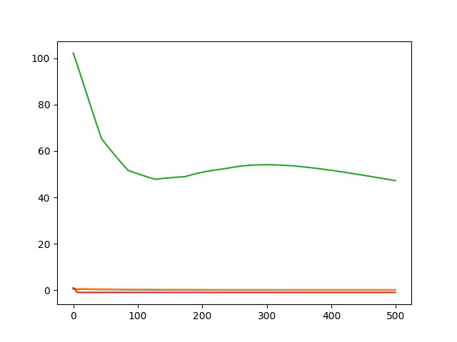
The example below demonstrates these 4 built-in regression metrics on a simple contrived regression problem.

from numpy import array
from keras.models import Sequential
from keras.layers import Dense
from matplotlib import pyplot
# prepare sequence
X = array([0.1, 0.2, 0.3, 0.4, 0.5, 0.6, 0.7, 0.8, 0.9, 1.0])
# create model
model = Sequential()
model.add(Dense(2, input_dim=1))
model.add(Dense(1))
model.compile(loss='mse', optimizer='adam', metrics=['mse', 'mae', 'mape', 'cosine'])
# train model
history = model.fit(X, X, epochs=500, batch_size=len(X), verbose=2)
# plot metrics
pyplot.plot(history.history['mean_squared_error'])
pyplot.plot(history.history['mean_absolute_error'])
pyplot.plot(history.history['mean_absolute_percentage_error'])
pyplot.plot(history.history['cosine_proximity'])
pyplot.show()

from numpy import array

from keras.models import Sequential

from keras.layers import Dense

from matplotlib import pyplot

# prepare sequence

X = array([0.1, 0.2, 0.3, 0.4, 0.5, 0.6, 0.7, 0.8, 0.9, 1.0])

# create model

model = Sequential()

model.add(Dense(2, input_dim=1))

model.add(Dense(1))

model.compile(loss='mse', optimizer='adam', metrics=['mse', 'mae', 'mape', 'cosine'])

# train model

history = model.fit(X, X, epochs=500, batch_size=len(X), verbose=2)

# plot metrics

pyplot.plot(history.history['mean_squared_error'])

pyplot.plot(history.history['mean_absolute_error'])

pyplot.plot(history.history['mean_absolute_percentage_error'])

pyplot.plot(history.history['cosine_proximity'])

pyplot.show()

Note: Your results may vary given the stochastic nature of the algorithm or evaluation procedure, or differences in numerical precision. Consider running the example a few times and compare the average outcome.

Running the example prints the metric values at the end of each epoch.

...
Epoch 96/100
0s - loss: 1.0596e-04 - mean_squared_error: 1.0596e-04 - mean_absolute_error: 0.0088 - mean_absolute_percentage_error: 3.5611 - cosine_proximity: -1.0000e+00
Epoch 97/100
0s - loss: 1.0354e-04 - mean_squared_error: 1.0354e-04 - mean_absolute_error: 0.0087 - mean_absolute_percentage_error: 3.5178 - cosine_proximity: -1.0000e+00
Epoch 98/100
0s - loss: 1.0116e-04 - mean_squared_error: 1.0116e-04 - mean_absolute_error: 0.0086 - mean_absolute_percentage_error: 3.4738 - cosine_proximity: -1.0000e+00
Epoch 99/100
0s - loss: 9.8820e-05 - mean_squared_error: 9.8820e-05 - mean_absolute_error: 0.0085 - mean_absolute_percentage_error: 3.4294 - cosine_proximity: -1.0000e+00
Epoch 100/100
0s - loss: 9.6515e-05 - mean_squared_error: 9.6515e-05 - mean_absolute_error: 0.0084 - mean_absolute_percentage_error: 3.3847 - cosine_proximity: -1.0000e+00

...

Epoch 96/100

0s - loss: 1.0596e-04 - mean_squared_error: 1.0596e-04 - mean_absolute_error: 0.0088 - mean_absolute_percentage_error: 3.5611 - cosine_proximity: -1.0000e+00

Epoch 97/100

0s - loss: 1.0354e-04 - mean_squared_error: 1.0354e-04 - mean_absolute_error: 0.0087 - mean_absolute_percentage_error: 3.5178 - cosine_proximity: -1.0000e+00

Epoch 98/100

0s - loss: 1.0116e-04 - mean_squared_error: 1.0116e-04 - mean_absolute_error: 0.0086 - mean_absolute_percentage_error: 3.4738 - cosine_proximity: -1.0000e+00

Epoch 99/100

0s - loss: 9.8820e-05 - mean_squared_error: 9.8820e-05 - mean_absolute_error: 0.0085 - mean_absolute_percentage_error: 3.4294 - cosine_proximity: -1.0000e+00

Epoch 100/100

0s - loss: 9.6515e-05 - mean_squared_error: 9.6515e-05 - mean_absolute_error: 0.0084 - mean_absolute_percentage_error: 3.3847 - cosine_proximity: -1.0000e+00

A line plot of the 4 metrics over the training epochs is then created.

Line Plot of Built-in Keras Metrics for Regression

Note that the metrics were specified using string alias values [‘mse‘, ‘mae‘, ‘mape‘, ‘cosine‘] and were referenced as key values on the history object using their expanded function name.

We could also specify the metrics using their expanded name, as follows:

model.compile(loss='mse', optimizer='adam', metrics=['mean_squared_error', 'mean_absolute_error', 'mean_absolute_percentage_error', 'cosine_proximity'])

1	model.compile(loss='mse', optimizer='adam', metrics=['mean_squared_error', 'mean_absolute_error', 'mean_absolute_percentage_error', 'cosine_proximity'])

We can also specify the function names directly if they are imported into the script.

from keras import metrics
model.compile(loss='mse', optimizer='adam', metrics=[metrics.mean_squared_error, metrics.mean_absolute_error, metrics.mean_absolute_percentage_error, metrics.cosine_proximity])

1 2	from keras import metrics model.compile(loss='mse', optimizer='adam', metrics=[metrics.mean_squared_error, metrics.mean_absolute_error, metrics.mean_absolute_percentage_error, metrics.cosine_proximity])

You can also use the loss functions as metrics.

For example, you could use the Mean squared Logarithmic Error (mean_squared_logarithmic_error, MSLE or msle) loss function as a metric as follows:

model.compile(loss='mse', optimizer='adam', metrics=['msle'])

1	model.compile(loss='mse', optimizer='adam', metrics=['msle'])

Keras Classification Metrics

Below is a list of the metrics that you can use in Keras on classification problems.

Binary Accuracy: binary_accuracy, acc
Categorical Accuracy: categorical_accuracy, acc
Sparse Categorical Accuracy: sparse_categorical_accuracy
Top k Categorical Accuracy: top_k_categorical_accuracy (requires you specify a k parameter)
Sparse Top k Categorical Accuracy: sparse_top_k_categorical_accuracy (requires you specify a k parameter)

Accuracy is special.

Regardless of whether your problem is a binary or multi-class classification problem, you can specify the ‘accuracy‘ metric to report on accuracy.

Below is an example of a binary classification problem with the built-in accuracy metric demonstrated.

from numpy import array
from keras.models import Sequential
from keras.layers import Dense
from matplotlib import pyplot
# prepare sequence
X = array([0.1, 0.2, 0.3, 0.4, 0.5, 0.6, 0.7, 0.8, 0.9, 1.0])
y = array([0, 0, 0, 0, 0, 1, 1, 1, 1, 1])
# create model
model = Sequential()
model.add(Dense(2, input_dim=1))
model.add(Dense(1, activation='sigmoid'))
model.compile(loss='binary_crossentropy', optimizer='adam', metrics=['accuracy'])
# train model
history = model.fit(X, y, epochs=400, batch_size=len(X), verbose=2)
# plot metrics
pyplot.plot(history.history['accuracy'])
pyplot.show()

from numpy import array

from keras.models import Sequential

from keras.layers import Dense

from matplotlib import pyplot

# prepare sequence

X = array([0.1, 0.2, 0.3, 0.4, 0.5, 0.6, 0.7, 0.8, 0.9, 1.0])

y = array([0, 0, 0, 0, 0, 1, 1, 1, 1, 1])

# create model

model = Sequential()

model.add(Dense(2, input_dim=1))

model.add(Dense(1, activation='sigmoid'))

model.compile(loss='binary_crossentropy', optimizer='adam', metrics=['accuracy'])

# train model

history = model.fit(X, y, epochs=400, batch_size=len(X), verbose=2)

# plot metrics

pyplot.plot(history.history['accuracy'])

pyplot.show()

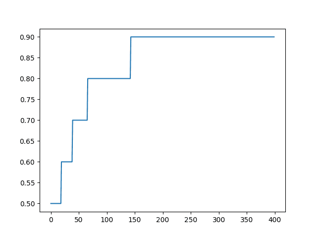
Running the example reports the accuracy at the end of each training epoch.

...
Epoch 396/400
0s - loss: 0.5934 - acc: 0.9000
Epoch 397/400
0s - loss: 0.5932 - acc: 0.9000
Epoch 398/400
0s - loss: 0.5930 - acc: 0.9000
Epoch 399/400
0s - loss: 0.5927 - acc: 0.9000
Epoch 400/400
0s - loss: 0.5925 - acc: 0.9000

...

Epoch 396/400

0s - loss: 0.5934 - acc: 0.9000

Epoch 397/400

0s - loss: 0.5932 - acc: 0.9000

Epoch 398/400

0s - loss: 0.5930 - acc: 0.9000

Epoch 399/400

0s - loss: 0.5927 - acc: 0.9000

Epoch 400/400

0s - loss: 0.5925 - acc: 0.9000

A line plot of accuracy over epoch is created.

Line Plot of Built-in Keras Metrics for Classification

Custom Metrics in Keras

You can also define your own metrics and specify the function name in the list of functions for the “metrics” argument when calling the compile() function.

A metric I often like to keep track of is Root Mean Square Error, or RMSE.

You can get an idea of how to write a custom metric by examining the code for an existing metric.

For example, below is the code for the mean_squared_error loss function and metric in Keras.

def mean_squared_error(y_true, y_pred):
    return K.mean(K.square(y_pred - y_true), axis=-1)

1 2	def mean_squared_error(y_true, y_pred): return K.mean(K.square(y_pred - y_true), axis=-1)

K is the backend used by Keras.

From this example and other examples of loss functions and metrics, the approach is to use standard math functions on the backend to calculate the metric of interest.

For example, we can write a custom metric to calculate RMSE as follows:

from keras import backend
 
def rmse(y_true, y_pred):
	return backend.sqrt(backend.mean(backend.square(y_pred - y_true), axis=-1))

from keras import backend

def rmse(y_true, y_pred):

return backend.sqrt(backend.mean(backend.square(y_pred - y_true), axis=-1))

You can see the function is the same code as MSE with the addition of the sqrt() wrapping the result.

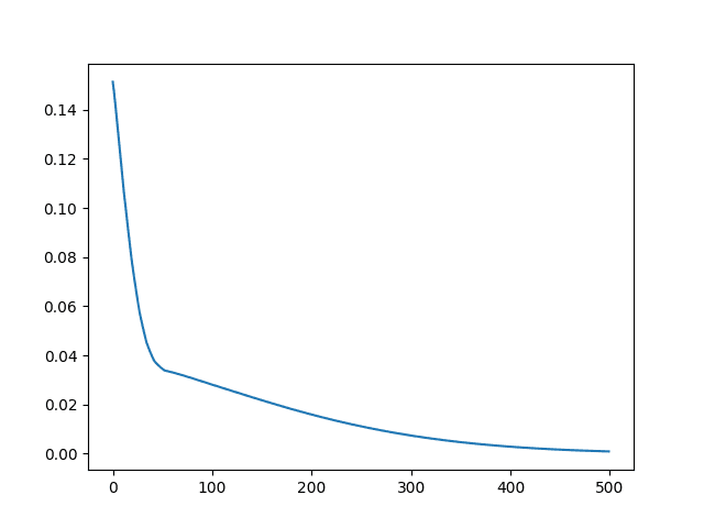
We can test this in our regression example as follows. Note that we simply list the function name directly rather than providing it as a string or alias for Keras to resolve.

from numpy import array
from keras.models import Sequential
from keras.layers import Dense
from matplotlib import pyplot
from keras import backend
 
def rmse(y_true, y_pred):
	return backend.sqrt(backend.mean(backend.square(y_pred - y_true), axis=-1))
 
# prepare sequence
X = array([0.1, 0.2, 0.3, 0.4, 0.5, 0.6, 0.7, 0.8, 0.9, 1.0])
# create model
model = Sequential()
model.add(Dense(2, input_dim=1, activation='relu'))
model.add(Dense(1))
model.compile(loss='mse', optimizer='adam', metrics=[rmse])
# train model
history = model.fit(X, X, epochs=500, batch_size=len(X), verbose=2)
# plot metrics
pyplot.plot(history.history['rmse'])
pyplot.show()

from numpy import array

from keras.models import Sequential

from keras.layers import Dense

from matplotlib import pyplot

from keras import backend

def rmse(y_true, y_pred):

return backend.sqrt(backend.mean(backend.square(y_pred - y_true), axis=-1))

# prepare sequence

X = array([0.1, 0.2, 0.3, 0.4, 0.5, 0.6, 0.7, 0.8, 0.9, 1.0])

# create model

model = Sequential()

model.add(Dense(2, input_dim=1, activation='relu'))

model.add(Dense(1))

model.compile(loss='mse', optimizer='adam', metrics=[rmse])

# train model

history = model.fit(X, X, epochs=500, batch_size=len(X), verbose=2)

# plot metrics

pyplot.plot(history.history['rmse'])

pyplot.show()

Running the example reports the custom RMSE metric at the end of each training epoch.

...
Epoch 496/500
0s - loss: 1.2992e-06 - rmse: 9.7909e-04
Epoch 497/500
0s - loss: 1.2681e-06 - rmse: 9.6731e-04
Epoch 498/500
0s - loss: 1.2377e-06 - rmse: 9.5562e-04
Epoch 499/500
0s - loss: 1.2079e-06 - rmse: 9.4403e-04
Epoch 500/500
0s - loss: 1.1788e-06 - rmse: 9.3261e-04

...

Epoch 496/500

0s - loss: 1.2992e-06 - rmse: 9.7909e-04

Epoch 497/500

0s - loss: 1.2681e-06 - rmse: 9.6731e-04

Epoch 498/500

0s - loss: 1.2377e-06 - rmse: 9.5562e-04

Epoch 499/500

0s - loss: 1.2079e-06 - rmse: 9.4403e-04

Epoch 500/500

0s - loss: 1.1788e-06 - rmse: 9.3261e-04

At the end of the run, a line plot of the custom RMSE metric is created.

Line Plot of Custom RMSE Keras Metric for Regression

Your custom metric function must operate on Keras internal data structures that may be different depending on the backend used (e.g. tensorflow.python.framework.ops.Tensor when using tensorflow) rather than the raw yhat and y values directly.

For this reason, I would recommend using the backend math functions wherever possible for consistency and execution speed.

Summary

In this tutorial, you discovered how to use Keras metrics when training your deep learning models.

Specifically, you learned:

How Keras metrics works and how you configure your models to report on metrics during training.
How to use classification and regression metrics built into Keras.
How to define and report on your own custom metrics efficiently while training your deep learning models.

Do you have any questions?
Ask your questions in the comments below and I will do my best to answer.

159 Responses to How to Use Metrics for Deep Learning with Keras in Python

Gerrit Govaerts August 9, 2017 at 5:03 pm #

Off topic but interesting none the less :
1) how to train an ensemble of models in the same time it takes to train 1
http://www.kdnuggets.com/2017/08/train-deep-learning-faster-snapshot-ensembling.html

2) when not to use deep learning
http://www.kdnuggets.com/2017/07/when-not-use-deep-learning.html

Reply
- Jason Brownlee August 10, 2017 at 6:51 am #
  
  Thanks for sharing.
  
  Reply
Olivier August 11, 2017 at 10:06 pm #

Hi Jason,

Thanks again for another great topic on keras but I’m a R user !

I can work with keras on R, but how about to implement custom metric ‘rmse’ on keras R please ?

Because I find something like that on the github repository :
metric_mean_squared_error <- function(y_true, y_pred) {
keras$metrics$mean_squared_error(y_true, y_pred)
}
attr(metric_mean_squared_error, "py_function_name") <- "mean_squared_error"

and my poor

rmse <- function(y_true, y_pred) {
K$sqrt(K$mean(K$square(y_pred – y_true)))
}

is not working ("nan" is returned)

Reply
- Olivier August 11, 2017 at 10:28 pm #
  
  Ok finally I make it return a value different from ‘nan’, but the result is not the same as the square root of ‘mse’ from keras ?!? Maybe due to the arg ‘axis = -1’ ?
  
  Reply
- Jason Brownlee August 12, 2017 at 6:46 am #
  
  Sorry, I have not used Keras in R, I don’t have good advice for you at this stage.
  
  Reply
John December 14, 2017 at 10:50 pm #

hi Jason,

Thanks for your very good topic on evaluation metrics in keras. can you please tell me how to compute macro-F and the micro-F scores?

thanks in advance

Reply
- Jason Brownlee December 15, 2017 at 5:33 am #
  
  Sorry, I am not familiar with those scores John.
  
  Perhaps find a definition and code them yourself?
  
  Reply
  - Stepan Lavrinenko February 16, 2020 at 4:10 am #
    
    Have you considered using the scikit-learn’s implementations? https://scikit-learn.org/stable/modules/generated/sklearn.metrics.f1_score.html
    Or would these not work with tensorflow?
    
    Reply
    - Jason Brownlee February 16, 2020 at 6:14 am #
      
      See here:
      https://machinelearningmastery.com/how-to-calculate-precision-recall-f1-and-more-for-deep-learning-models/
      
      Reply
Linda Cen December 22, 2017 at 5:26 am #

Hi Jason,

I used your “def rmse” in my code, but it returns the same result of mse.

# define data and target value
X = TFIDF_Array
Y = df[‘Shrinkage’]

# custom metric to calculate RMSE
def RMSE(y_true, y_pred):
return backend.sqrt(backend.mean(backend.square(y_pred – y_true), axis=-1))

# define base model
def regression_model():
# create model
model = Sequential()
model.add(Dense(512, input_dim=X.shape[1], kernel_initializer=’uniform’, activation=’relu’))
model.add(Dropout(0.5))
model.add(Dense(1, kernel_initializer=’uniform’))
# compile model
model.compile(loss=’mse’, optimizer=’sgd’, metrics=[RMSE])
return model

# evaluate model
estimator = KerasRegressor(build_fn=regression_model, nb_epoch=100, batch_size=32, verbose=0)
kfold = KFold(n_splits=3, random_state=1)
reg_results = cross_val_score(estimator, X, Y, cv=kfold)

Reply
- Jason Brownlee December 22, 2017 at 5:37 am #
  
  Did the example in the post – copied exactly – work for you?
  
  Reply
  - Linda Cen December 22, 2017 at 8:58 am #
    
    Epoch 496/500
    0s – loss: 3.9225e-04 – rmse: 0.0170
    Epoch 497/500
    0s – loss: 3.8870e-04 – rmse: 0.0169
    Epoch 498/500
    0s – loss: 3.8518e-04 – rmse: 0.0169
    Epoch 499/500
    0s – loss: 3.8169e-04 – rmse: 0.0168
    Epoch 500/500
    0s – loss: 3.7821e-04 – rmse: 0.0167
    
    It gave back different values from yours.
    
    Reply
    - Linda Cen December 22, 2017 at 9:04 am #
      
      Epoch 497/500
      0s – loss: 0.0198 – mean_squared_error: 0.0198
      Epoch 498/500
      0s – loss: 0.0197 – mean_squared_error: 0.0197
      Epoch 499/500
      0s – loss: 0.0197 – mean_squared_error: 0.0197
      Epoch 500/500
      0s – loss: 0.0196 – mean_squared_error: 0.0196
      
      and these were the result when I used:
      metrics=[‘mean_squared_error’]
      
      I didn’t see any difference of MSE and RMSE here.
      
      Please advise. Thanks.
      
      Reply
    - Jason Brownlee December 22, 2017 at 4:15 pm #
      
      Yes, this is to be expected. Machine learning algorithms are stochastic meaning that the same algorithm on the same data will give different results each time it is run. See this post for more details:
      https://machinelearningmastery.com/randomness-in-machine-learning/
      
      Reply
lila January 30, 2018 at 5:19 am #

Dear Jason,
Thank you again for the awsome blog and clear explanations
If I understood well, RMSE should be equal to sqrt(mse), but this is not the case for my data:
Epoch 130/1000

10/200 [>………………………..] – ETA: 0s – loss: 0.0989 – rmse: 0.2656
200/200 [==============================] – 0s 64us/step – loss: 0.2856 – rmse: 0.4070

Please sir, how can we calculate the coefficient of determination

Reply
- Jason Brownlee January 30, 2018 at 9:56 am #
  
  The mse may be calculated at the end of each batch, the rmse may be calculated at the end of the epoch because it is a metric.
  
  Reply
  - Josh Park March 27, 2019 at 11:14 am #
    
    Hi Jason, thanks for the helpful blog. Quick question regarding your reply here, if the rmse metric is calculated at the end of each epoch, why is it constantly being updated during an epoch whenever you’re training?
    
    Reply
    - Jason Brownlee March 27, 2019 at 2:06 pm #
      
      It is calculated/estimated per batch I believe.
      
      Reply
      - Josh Park March 27, 2019 at 10:47 pm #
        
        Thanks for your reply. If that’s the case, why is the square root of the MSE loss function not equal to the RMSE metric value from above if they are both calculated at the end of each batch?
      - Jason Brownlee March 28, 2019 at 8:15 am #
        
        They should be, and if not, then there is a difference in the samples used to calculate the score – e.g. batch vs epoch, or a difference in precision between the two calculations causing rounding errors.
        
        You could try digging into the code if this matters.
        
        Generally, I recommend a separate standalone evaluation of model performance and only use training values as a rough/directional assessment.
lila January 30, 2018 at 5:26 am #

For the determination coefficient I use this basic code

S1, S2 = 0, 0
for i in range(len(Y)):
S1 = S1 + (Y_pred_array[i] – mean_y)**2
S2 = S2 + (Y_array[i] – mean_y)**2

R2 = S1/S2

But this gives give bad results

Reply
- Walid March 6, 2018 at 6:21 am #
  
  How can you deal with Y_pred as iterable also it is a Tensor?
  
  Thanks
  
  Reply
- Amilkar Herrera January 8, 2021 at 4:06 pm #
  
  I’ve been having this same problem. Readin the documentation you can see that by default, the metrics are evaluated by batch and the averaged.
  
  “In this case, the scalar metric value you are tracking during training and evaluation is the average of the per-batch metric values for all batches see during a given epoch (or during a given call to model.evaluate()).”
  
  For the details, see https://keras.io/api/metrics/
  
  Reply
  - Jason Brownlee January 9, 2021 at 6:38 am #
    
    My advice is to calculate the metric manually via the evaluate() function to get a true estimate of model performance.
    
    Any scores reporting during training are just a rough approximation.
    
    Reply
sam February 28, 2018 at 5:58 pm #

Thanks for the article. How does Keras compute a mean statistic in a per batch fashion? Does it internally (magically) aggregate the sum and count to that point in the epoch and print the measure or does it compute the measure per batch and then again re-compute the metric at the end of each epoch over the entire data?

Reply
- Jason Brownlee March 1, 2018 at 6:09 am #
  
  I believe the sum is accumulated and printed at the end of each batch or end of each epoch. I don’t recall which.
  
  Reply
Walid March 6, 2018 at 6:18 am #

Great post and just in time as usual;

The issue is that I am trying to calculate the loss based on IoU (Intersection over union) and I have no clue how to do it using my backend (TensorFlow)
My output is like this(xmin,ymin,xmax,ymax)

Thanks

Reply
- Jason Brownlee March 6, 2018 at 6:20 am #
  
  Sorry, I have not implemented (or heard of) that metric.
  
  Reply
MLT March 8, 2018 at 8:39 am #

model.compile(loss=’mse’, optimizer=’adam’, metrics=[rmse])

Epoch 496/500
0s – loss: 1.2992e-06 – rmse: 9.7909e-04

loss is mse. Should mse = rmse^2? Above value (9.7909e-04)^2 is 9.6e-8, which mismatch 1.2992e-06. Did I misunderstand something? Thanks.

Reply
- Jason Brownlee March 8, 2018 at 2:54 pm #
  
  The loss and metrics might not be calculated at the same time, e.g. end of batch vs end of epoch.
  
  Reply
  - MLT March 9, 2018 at 8:06 am #
    
    Thanks for reply.
    
    history = model.fit(X, X, epochs=500, batch_size=len(X), verbose=2)
    I thought the duration of batch is equal to one epoch, since batch_size=len(X). If it is correct?
    
    Furthermore, it seems that the loss of epoch is also updated each iteration.
    
    Epoch 496/500
    0s – loss: 1.2992e-06 – rmse: 9.7909e-04
    
    Reply
    - Jason Brownlee March 10, 2018 at 6:13 am #
      
      No, one epoch is comprised of 1 or more batches. Often 32 samples per batch are used as a default.
      
      Lear more here:
      https://machinelearningmastery.com/gentle-introduction-mini-batch-gradient-descent-configure-batch-size/
      
      Reply
      - MLT March 10, 2018 at 7:38 am #
        
        Thanks a lot for your time to explain and find the link.
        
        I am sorry. I think I did not express my thoughts correctly.
        
        In the above example, history = model.fit(X, X, epochs=500, batch_size=len(X), verbose=2)
        
        batch_size=len(X)
        batch_size: Integer or None. Number of samples per gradient update. If unspecified, batch_size will default to 32.
        
        Since batch_size has been specified as the length of testset, may I consider one epoch comprises 1 batch and the end of a batch is the time when an epoch is end? Model ’mse’ loss is the rmse^2.
      - Jason Brownlee March 11, 2018 at 6:15 am #
        
        Yes, correct.
kazim March 13, 2018 at 8:58 pm #

Thanks for the great article, Jason. I have 2 questions;

1) I have a pipeline which has a sequence like : Normalizer –> KerasRegressor
Can I simply use history = pipeline.fit(..) then plot metrics ?

2) I have a KFold crossvalidation like that:
kfold = StratifiedKFold(n_splits=3)
results = cross_val_score(pipeline, X, Y, cv=kfold, scoring = mape)
How I can plot that 3 CV fits’ metrics?

Thanks.

Reply
- Jason Brownlee March 14, 2018 at 6:19 am #
  
  No, I don’t believe you can easily access history when using the sklearn wrappers.
  
  Reply
George Kibirige March 29, 2018 at 7:42 pm #

HI Dr. Jason Brownlee

Thanks for good tutorial.

What is the different between these two lines
score = model.evaluate(data2_Xscaled, data2_Yscaled, verbose=verbose)
y_hat = model.predict(data2_Xscaled)

objective metric is the customized one def rmse(y_true, y_pred)

the score value should also equal to y_hat

Reply
- Jason Brownlee March 30, 2018 at 6:35 am #
  
  One evaluates the model the other makes a prediction.
  
  Reply
GARCIA LOPEZ ALFONSA April 24, 2018 at 9:21 pm #

Hello Jason,
Thanks for your work.

I’m using MAE as metric in a multi-class classification problem with ordered classes.
Because, in my problem it is not the same to classify a record of class 5 in the class 4, than to assign it to the class 1.

My model is:

network %
layer_dense(units = 32, activation = “relu”, input_shape = c(38)) %>%
layer_dense(units = 5, activation = “softmax”)

network %>% compile(
optimizer = “rmsprop”,
loss = “categorical_crossentropy”,
metrics = c(“mae”)
)

But the model does not correctly calculate the MAE.

It is possible to use MAE for this classification problem?

Tanks

Reply
- Jason Brownlee April 25, 2018 at 6:23 am #
  
  MAE is not an appropriate measure of error for classification, it is intended for regression problems.
  
  You can learn the difference between classification and regression here:
  https://machinelearningmastery.com/faq/single-faq/what-is-the-difference-between-classification-and-regression
  
  Reply
Ashwin July 7, 2018 at 2:28 pm #

Do you have a code written for the mean_iou metric?

Reply
- Jason Brownlee July 8, 2018 at 6:15 am #
  
  What is mean_iou?
  
  Reply
Zahoor July 23, 2018 at 7:10 pm #

Hi Jason,

When defining a custom metrics function, the y_true and y_pred are of type Tensor. If I have my own function that takes numpy arrays as input how do I convert y_true and y_pred to numpy arrays?

Reply
- Jason Brownlee July 24, 2018 at 6:13 am #
  
  You will need to work with Tensor types. That is the expectation of Keras.
  
  Reply
Anam August 11, 2018 at 8:04 pm #

Dear Jason,
How can we use precision and recall metrics for Deep Learning with Keras in Python?
Thanx in advance.

Reply
- Jason Brownlee August 12, 2018 at 6:32 am #
  
  You can make predictions with our model then use the precision and recall metrics from the sklearn library.
  
  Reply
Omar August 30, 2018 at 8:17 pm #

Hello mr Jason
I have a question that have confused me for so long.
For a multiple output regression problem, what does the MSE loss function compute exactly ?
Thank you in advance.

Reply
Nitin Pasumarthy September 1, 2018 at 3:47 am #

Nice article(s) Jason.
At run time, I wanted to bucket the classes and evaluate. So tried this function but it returns nan.

def my_metric(y_true, y_pred):
actual = tf.floor( y_true / 10 )
predicted = tf.floor( y_pred / 10 )
return K.categorical_crossentropy(actual, predicted)

Reply
- Jason Brownlee September 1, 2018 at 6:22 am #
  
  Sorry, I cannot debug your code. Perhaps post to stackoverflow?
  
  Reply
- Nitin Pasumarthy September 1, 2018 at 9:06 am #
  
  Sorry. Thanks a lot. Learned some good things 🙂
  
  Reply
Omar September 26, 2018 at 1:56 am #

Hello mr Jason
For a multiple output regression problem, what does the MSE loss function compute exactly ?
Is it the sum of the MSE over all the output variables, the average or something else ?
Thank you in advance.

Reply
- Jason Brownlee September 26, 2018 at 6:17 am #
  
  The average of the squared differences between model predictions and true values.
  
  Reply
  - Omar October 1, 2018 at 2:36 am #
    
    This is for just one output, what if I have multiple outputs ?
    
    Reply
    - Jason Brownlee October 1, 2018 at 6:27 am #
      
      You can calculate the metric for each time step or output. I have an example here:
      https://machinelearningmastery.com/multi-step-time-series-forecasting-long-short-term-memory-networks-python/
      
      Reply
JG September 30, 2018 at 2:39 am #

Thank you so much for your Tutorial. Nowadays I follow your twitter proposals everyday. It’s great !

I have two questions:

1) regarding sequential model in the last example;
if I remove activation definition = ‘relu’, in your last code example … I got a surprising better RMSE performance values… it is suggest to me that has something to do with Regression issues that works better if we do not put activation at all in the first hide layer. Is it casual result or any profound reason?

2) using a same architectural model, which is better a Regression approach (we leave out the activation in the output layer) or a multinomial classification (we set up the appropriate ‘softmax’ as activation in the output layer), imagine for example, we analyze same problem, e.g. we have all continuos label output or any discrete multiclass label (for getting for example rounded real number by their equivalent integer number), for a serie of real number samples …I mean is there any intrinsic advantage or behavior using Regression analysis vs Multinomial classification ?

thanks
JG

Reply
- Jason Brownlee September 30, 2018 at 6:07 am #
  
  It really depends on the problem as to the choice and benefit of activation functions.
  
  In terms of activation in the output layer – what I think you’re asking about, the heuristics are:
  
  – regression: use ‘linear’
  – binary classification: use ‘sigmoid’
  – multi-class classification: use ‘softmax’.
  
  Does that help?
  
  Reply
JG September 30, 2018 at 8:20 am #

If I imagine a continuos curve for a linear regression as output of prediction vs imagine for the same problem different outputs of segments to categorize a big multi-class classification, using the same main model architecture (obviously with different units and activation at output, loss and metrics at compilation, etc) …which model will perform better the regression or the multi-class (for the same problem approach) ?
My intuition tell me that multi-class it is more fine because it can focus on specific segment output (classes) of the linear regression curve (and even it has more units at the output therefore more analysis it is involved. Do not worry to much, I try in the future to experiment with some specific examples, to search for my question.

Anyway, do you like women basket? congratulations Australia won to España (-Spain it is my country -) two hours ago…

Reply
- Jason Brownlee October 1, 2018 at 6:23 am #
  
  I don’t follow, sorry.
  
  A classification model is best for classification and will perform beyond poorly for regression.
  
  Not a sports guy, sorry 🙂
  
  Reply
Ronny November 2, 2018 at 4:53 am #

Thanks for the tutorial.

I followed all of the steps and used my own metric function successfully. I was also able to plot it.

The problem that I encountered was when I tried to load the model and the saved weights in order to use model.evaluate_generator(). I keep getting the error: “Exception has occurred: ValueError too many values to unpack (expected 2) ”

I was wondering if you know how to solve this problem.

Reply
- Jason Brownlee November 2, 2018 at 5:59 am #
  
  I have not seen this. Is your version of Keras up to date? v2.2.4 or better?
  
  Reply
Paul A. Gureghian November 4, 2018 at 9:08 am #

How to extract and store the accuracy output from ‘loss’ and ‘metrics’ in the model.compile step in order to pass those float values to mlflow’s log_metric() function ?

Reply
Paul A. Gureghian November 4, 2018 at 9:10 am #

history = regr.compile(optimizer, loss = ‘mean_squared_error’, metrics =[‘mae’])

My ‘history’ variable keeps coming up as ‘None type’

Reply
- Jason Brownlee November 5, 2018 at 6:07 am #
  
  That is odd, I have not seen that before.
  
  Perhaps post to the keras user group:
  https://machinelearningmastery.com/get-help-with-keras/
  
  Reply
Orion November 5, 2018 at 12:46 am #

Hi Dr. Brownlee,

By definition, rmse should be square root of mse.

But if we fit keras with batches, rmse would not be calculated correctly.

Could you give me some advices about how to use customized rmse metric with batches fitting properly?

Reply
- Jason Brownlee November 5, 2018 at 6:16 am #
  
  If you add RMSE as a metric, it will be calculated at the end of each epoch, i.e. correctly.
  
  Reply
Rohan November 8, 2018 at 4:26 am #

Why is the cosine proximity value negative in this case. Should it not be positive since the dot product computed is of the same vectors it should be +1.0 right?

Reply
- Jason Brownlee November 8, 2018 at 6:13 am #
  
  Perhaps because the framework expects to minimize loss.
  
  Reply
  - Rohan November 8, 2018 at 7:03 am #
    
    What would be the correct interpretation of negative value in this case? In the example you have mentioned since both the vectors were same the value we received was -1.0. When i google the meaning of it certain blogs mentioned that it means that vector are similar but in opposite directions . This does not seem a correct interpretation as both vectors are same
    
    Reply
    - Jason Brownlee November 8, 2018 at 2:11 pm #
      
      Sorry, i don’t have material on this measure, perhaps this will help:
      https://en.wikipedia.org/wiki/Cosine_similarity
      
      Reply
Jenna Ma December 24, 2018 at 9:47 pm #

This post helps me again. You are the best. 🙂
I have a question when I write the custom metrics for my project.
Assuming that g and v are two inputs of the model, and v in the next time step is output. There is a relationship between g and v. The loss function of the model is MSE of the output. But when it comes to the metrics, I want to define it as the MSE of predicted g and observed g.
When I write a custom metric to calculate the MSE, I don’t know how to make y_true represents the observed g.
Did I make it clear?
Thank you in advance.

Reply
- Jason Brownlee December 25, 2018 at 7:21 am #
  
  It might be easier to write a custom function and evaluate model performance manually.
  
  Reply
  - Jenna Ma December 26, 2018 at 5:40 pm #
    
    Thank you for the advice.
    I use the method you introduced in another post: https://machinelearningmastery.com/implement-machine-learning-algorithm-performance-metrics-scratch-python/
    It works.
    Thanks a lot!
    
    Reply
    - Jason Brownlee December 27, 2018 at 5:40 am #
      
      Well done!
      
      Reply
Jimmy Tsao December 25, 2018 at 8:25 pm #

I’m trying to build my own accuracy function that checks if the output sequence is same as the true answer . For example if the true answer is ” 0.2 0.4 0.6 0.8 ”, either ” 0.4 0.6 0.8 0.2” or ”0.8 0.6 0.4 0.2 ” will be define as correct. Do you have any thoughts or recommendations?

Reply
- Jason Brownlee December 26, 2018 at 6:42 am #
  
  You would not use accuracy, you would use an error, such as MSE, MAE or RMSE.
  
  Reply
  - Jimmy Tsao December 26, 2018 at 2:27 pm #
    
    But I would like the out come be 1’s and 0’s not in the middle. Will that be possible?
    Also merry Christmas, forgot that yesterday.
    
    Reply
    - Jason Brownlee December 27, 2018 at 5:39 am #
      
      You can round a floating point value to either 0/1.
      
      Reply
Jenna Ma December 27, 2018 at 7:20 pm #

I did not find any post in your blog specifically focus on loss function, so I submit my question under this post.
There are two output features in my model. I’m not sure how the loss function works. Whether the loss function returns the sum of two calculated errors or weighted sum or some other values?
MSE = MSEa + MSEb ?
MSE = 0.5*MSEa + 0.5*MSEb ?
If it returns the weighted sum, can I define the weight?
Thank you in advance.

Reply
- Jason Brownlee December 28, 2018 at 5:55 am #
  
  You can choose how to manage how to calculate loss on multiple outputs.
  
  Adding a constant 1 or 0.5 does not make any difference in practice, I would imagine.
  
  Reply
Ayhan December 30, 2018 at 11:53 pm #

Hi Dr.Brownlee,
I want to define custom monitor metrics such as AUC for Early Stopping and ModelCheckpoint and other callbacks for monitor options and metrics for model.compile,
What do i do ?

I’m looking forward to your answer.

Thanks,

Reply
- Jason Brownlee December 31, 2018 at 6:11 am #
  
  Create a list of callbacks and pass it to the “callbacks” argument on the fit() function.
  
  Reply
Solo January 7, 2019 at 3:23 pm #

Thanks for the tutorials.
Precision and Recall metrics have been removed from the latest version of keras, they cited that the metric was misleading, do you have any idea how to create a custom precision and recall metrics?

Reply
- Jason Brownlee January 8, 2019 at 6:44 am #
  
  Yes, you can make predictions with your model then calculate the metrics with sklearn:
  https://scikit-learn.org/stable/modules/classes.html#module-sklearn.metrics
  
  Reply
Asal January 28, 2019 at 3:31 pm #

Thank you so much for your tutorials.

I want to write a costume metric function. This function is PSNR (Peak signal-to-noise ratio) which is most commonly used to measure the quality of reconstruction of lossy compression codecs. My loss function is MSE.

PSNR is calculated based on the MSE results. So I was wondering if there is a way to write this PSNR function using the loss that is calculated in the fitting process. Or I should calculate MSE in the body of the function and use that information to calculate PSNR.

Also, In your code:

def rmse(y_true, y_pred):
return backend.sqrt(backend.mean(backend.square(y_pred – y_true), axis=-1))

What are the inputs of rmse during the training? How it is assigning y_true and y_pred?

Reply
- Jason Brownlee January 29, 2019 at 6:08 am #
  
  The inputs to the function are the true y values and the predicted y values.
  
  Reply
  - Asal January 30, 2019 at 9:22 am #
    
    Thank you so much for your response, Jason.
    
    This custom metric should return a tensor, right?
    
    I had to use log10 in my computations. But then Keras only has log of e. (tf.keras.backend.log(x))
    
    So I used math.log10 and I was getting an error in model.compile(). Here is the previous code:
    
    def PSNR(y_true, y_pred):
    
    max_I = 1.0
    
    return 20*math.log10(max_I) – 10*math.log10( backend.mean( backend.square(y_pred – y_true),axis=-1)
    
    Then, I thought I can use numpy to calculate the last line and then make a tensor of the result.
    
    So I changed my code to:
    
    def PSNR(y_true, y_pred):
    
    max_I = 1.0
    val = 20*math.log10(max_I) – 10*math.log10(np.mean( np.square(y_pred – y_true),axis=-1))
    newTensor = K.variable(value = val)
    return newTensor
    
    I’m not getting any error. But is this the right way to do this?
    
    Reply
    - Jason Brownlee January 30, 2019 at 2:40 pm #
      
      Yes, you must operate upon tensors.
      
      Sorry, I don’t have the capacity to review/debug your approach.
      
      Reply
      - Asal January 31, 2019 at 6:41 am #
        
        Thank you, Jason.

Niraj March 1, 2019 at 2:04 am #

from numpy import array
from keras.models import Sequential
from keras.layers import Dense
from matplotlib import pyplot
# prepare sequence
X = array([0.1, 0.2, 0.3, 0.4, 0.5, 0.6, 0.7, 0.8, 0.9, 1.0])
y = array([0, 0, 0, 0, 0, 1, 1, 1, 1, 1])
# create model
model = Sequential()
model.add(Dense(2, input_dim=1))
model.add(Dense(1, activation='sigmoid'))
model.compile(loss='binary_crossentropy', optimizer='adam', metrics=['sparse_categorical_accuracy'])
# train model
history = model.fit(X, y, epochs=40, batch_size=len(X), verbose=2)
# plot metrics
acc = history.history['sparse_categorical_accuracy']
val_acc = history.history['val_acc']
epochs = range(1, len(acc) + 1)
pyplot.plot(epochs,acc, 'bo', label='Training acc')
pyplot.title('Training and validation accuracy')
pyplot.legend()
pyplot.tight_layout()
pyplot.show()

Epoch 39/40
 - 0s - loss: 0.6356 - sparse_categorical_accuracy: 0.5000
Epoch 40/40
 - 0s - loss: 0.6353 - sparse_categorical_accuracy: 0.5000
---------------------------------------------------------------------------
KeyError                                  Traceback (most recent call last)
 in ()
     15 # plot metrics
     16 acc = history.history['sparse_categorical_accuracy']
---> 17 val_acc = history.history['val_acc']
     18 epochs = range(1, len(acc) + 1)
     19 pyplot.plot(epochs,acc, 'bo', label='Training acc')

KeyError: 'val_acc'

from numpy import array

from keras.models import Sequential

from keras.layers import Dense

from matplotlib import pyplot

# prepare sequence

X = array([0.1, 0.2, 0.3, 0.4, 0.5, 0.6, 0.7, 0.8, 0.9, 1.0])

y = array([0, 0, 0, 0, 0, 1, 1, 1, 1, 1])

# create model

model = Sequential()

model.add(Dense(2, input_dim=1))

model.add(Dense(1, activation='sigmoid'))

model.compile(loss='binary_crossentropy', optimizer='adam', metrics=['sparse_categorical_accuracy'])

# train model

history = model.fit(X, y, epochs=40, batch_size=len(X), verbose=2)

# plot metrics

acc = history.history['sparse_categorical_accuracy']

val_acc = history.history['val_acc']

epochs = range(1, len(acc) + 1)

pyplot.plot(epochs,acc, 'bo', label='Training acc')

pyplot.title('Training and validation accuracy')

pyplot.legend()

pyplot.tight_layout()

pyplot.show()

Epoch 39/40

- 0s - loss: 0.6356 - sparse_categorical_accuracy: 0.5000

Epoch 40/40

- 0s - loss: 0.6353 - sparse_categorical_accuracy: 0.5000

---------------------------------------------------------------------------

KeyError Traceback (most recent call last)

in ()

15 # plot metrics

16 acc = history.history['sparse_categorical_accuracy']

---> 17 val_acc = history.history['val_acc']

18 epochs = range(1, len(acc) + 1)

19 pyplot.plot(epochs,acc, 'bo', label='Training acc')

KeyError: 'val_acc'

How do I resolve this error message? Please help!

Jason Brownlee March 1, 2019 at 6:25 am #

In order to access val_acc you must fit the model with a validation dataset. e.g. set validation_data=(…) in the call to model.fit(…)

Reply

krishna March 4, 2019 at 11:17 pm #

can a target value for mse can be given?
can the system be tested for convergence

Reply
- Jason Brownlee March 5, 2019 at 6:40 am #
  
  This is a common question that I answer here:
  https://machinelearningmastery.com/faq/single-faq/how-to-know-if-a-model-has-good-performance
  
  Reply
Ben March 6, 2019 at 9:01 am #

Hi Jason,

Is there ever a limit to number of epochs? In my data set (regression) the more epochs the better the model keeps performing… Even past 500… Is anything over 2000 epochs odd??

Reply
- Jason Brownlee March 6, 2019 at 2:44 pm #
  
  Not really.
  
  Reply
  - ben March 7, 2019 at 1:13 am #
    
    In regression… Ideally when should one stop adding epochs? Is it possible to verify just thru an RSME plot?
    
    Reply
    - Jason Brownlee March 7, 2019 at 6:54 am #
      
      When the model no longer improves on the holdout validation dataset.
      
      Reply
R April 22, 2019 at 12:22 am #

Hi Jason,

in the codes of Custom Metrics in Keras part, you defined the rmse function as follow:

def rmse(y_true, y_pred):
return backend.sqrt(backend.mean(backend.square(y_pred – y_true), axis=-1))

Why is it necessary to write axis=-1? I don’t understand what axis=-1 means here.
I deleted axis=-1 from the function in my codes but it is still OK to run?

Reply
- Jason Brownlee April 22, 2019 at 6:25 am #
  
  It is explicitly specifying to calculate the error across the last dimension, normally this is samples, but for encoder-decoder lstms this will be time steps.
  
  Reply
Belgian_student May 15, 2019 at 10:17 am #

Hello Mr. Brownlee,

-> Thanks for this tutorial, you helped me a lot.

For my thesis, I did a regression cnn in keras using the four metrics you present here to be interesting for regression.

I’ve this question with respect to the cosine_proximity-metric: if the vectors in nominator and denominator of the underlying formula are 1-dimensional vectors (=being just the real valued true and predicted label), then the metric will always resolve to 1?

– Why is its use then so interesting for regression networks, or maybe networks with multiple regressed output are intended here?

– Have you got any idea how its value could be ‘-1’ instead of ‘+1’ when both the true and predicted label are positive?

Kind Regards from Belgium

Reply
- Jason Brownlee May 15, 2019 at 2:45 pm #
  
  Sorry, I can’t give you good off the cuff about the cosine similarity metric.
  
  I hope to cover it in the future.
  
  Reply
Elena June 16, 2019 at 12:05 am #

Hi!
I am trying to train a recurrent neural network implemented using Keras and mean square error as loss function. Is it possible to have a loss greater than 1 and the model generated by the network to work as expected?

Reply
- Jason Brownlee June 16, 2019 at 7:13 am #
  
  Perhaps.
  
  Reply
shiva July 25, 2019 at 11:31 am #

When i try to use a model saved using rmse as metric.
During loading the model
load_model(….),,,
it gives the following error
ValueError: Unknown metric function:rmse

What is the best metric for timeseries data?
My model with MSE is either good in capturing higher signals or either fails to capture low signals..
I want a better metric which would preserve correlation and MSE together..

thank you

Reply
- Jason Brownlee July 25, 2019 at 2:11 pm #
  
  Good question, you must provide a dict to the load_model() function that indicates what the rmse function means.
  
  For example, and assuming the rmse function is defined:
  
  model = load_model('model.h4', custom_objects={'rmse':rmse})
  
  1
  
  model = load_model('model.h4', custom_objects={'rmse':rmse})
  
  Reply
  - shiva July 26, 2019 at 12:39 am #
    
    Thanks for the reply but i still have an error.
    
    IndexError: tuple index out of range
    
    C:\ProgramData\Anaconda3\lib\site-packages\numpy\core\_methods.py in _count_reduce_items(arr, axis)
    53 items = 1
    54 for ax in axis:
    —> 55 items *= arr.shape[ax]
    56 return items
    57
    
    IndexError: tuple index out of range
    
    Reply
    - Jason Brownlee July 26, 2019 at 8:26 am #
      
      Sorry to hear that. I don’t have any good ideas.
      
      Perhaps try searching/posting stackoverflow?
      
      Reply
shiva July 26, 2019 at 12:05 am #

What is the best metric for timeseries data?
My model with MSE is either good in capturing higher signals or either fails to capture low signals..

I want a better metric which would preserve correlation and MSE together..

Reply
- Jason Brownlee July 26, 2019 at 8:26 am #
  
  I find RMSE or MAPE useful.
  
  Reply
Anand August 20, 2019 at 1:05 am #

Very informative blog. But can you please tell me how to use recall as a metric.

Reply
- Jason Brownlee August 20, 2019 at 6:27 am #
  
  Just plug it in to the above examples.
  
  Reply
Alex September 7, 2019 at 10:15 am #

Hello Sir.

Please if I’ve normalized my dataset ( X and Y), with MinMaxScaler for example, and if I’m using MSE or RMSE for loss and/or for metrics, the results expected (mse and rmse) are also normalized, right?

How can I get the “real” MSE and RMSE of the original data (X and Y) denormalized?

Thanks much in advance.

Reply
- Jason Brownlee September 8, 2019 at 5:12 am #
  
  Correct.
  
  You can get real error by inverting the transform on the predictions first, then calculating error metrics. The objects typically offer an inverse_transform() function.
  
  Reply
  - Alex September 12, 2019 at 6:36 am #
    
    Ok. Right. I did it. Thanks! One more question please…
    
    But how about if I, let’s say, normalize X and standardize Y, or vice-versa.
    
    When inverting the transformation on the predictions [predict(X_test) = Y_pred], which scaler should I use to get the “real” Y_pred inversely transformed?
    
    The inverse of normalized or the inverse of standardized?
    
    You know what I mean?
    
    Thanks much in advance.
    
    Reply
    - Jason Brownlee September 12, 2019 at 1:46 pm #
      
      You invert the transforms applied to y, in the reverse order in which they were applied.
      
      This may give you some ideas:
      https://machinelearningmastery.com/machine-learning-data-transforms-for-time-series-forecasting/
      
      Reply
benjamin appiah October 12, 2019 at 5:09 pm #

I tried using a custom loss function but always fall into errors.

Mahalanobis distance (or “generalized squared interpoint distance” for its squared value[3]) can also be defined as a dissimilarity measure between two random vectors x and y of the same distribution with the covariance matrix S.
d(x,y) = square [Transpose(x-y) * Inverse(S)* (x-y)]
(https://en.wikipedia.org/wiki/Mahalanobis_distance)

n_classes = 4
n_samples=800
X, y = make_classification(n_samples=n_samples, n_features=20, n_informative=4, n_redundant=0, n_classes=n_classes, n_clusters_per_class=2)
y = to_categorical(y)
Xtrainb, testXb, ytrainb, ytestb = train_test_split(X, y, test_size = 0.3, random_state=42)

x_trainb = np.reshape(Xtrainb, (Xtrainb.shape[0], Xtrainb.shape[1], 1))
Xtestb = np.reshape(testXb, (testXb.shape[0], testXb.shape[1], 1))

densesize = 4
input_datab = Input(shape=(Xtrainb.shape[1],1))
epochs = 10
batch_size = 32

########
def mahalanobis(y_true, y_pred):
x_minus_mn_with_transpose = K.transpose(y_true – y_pred)
Covariance = covr1(y_true, y_pred)
inv_covmat = tf.linalg.inv(Covariance)
x_minus_mn = y_true – y_pred
left_term = K.dot(x_minus_mn, inv_covmat)
D_square = K.dot(left_term, x_minus_mn_with_transpose)
return D_square

def covr1(y_true, y_pred):
#x_mean = K.mean(y_true)
#y_mean = K.mean(y_pred)
Cov_numerator = K.sum(((y_true – y_pred)*(y_true – y_pred)))
Cov_denomerator = len(Xtrainb)-1
Covariance = (Cov_numerator / Cov_denomerator)
return Covariance

conv1= Conv1D(filters=80, kernel_size=2, padding=’same’, input_dim=Xtrainb.shape[1])(input_datab)
maxpool = MaxPooling1D(pool_size=3, stride=3 )(conv1)
conv2= Conv1D(filters=50, kernel_size=2, padding=’same’, input_dim=Xtrainb.shape[1])(maxpool)
maxpool = MaxPooling1D(pool_size=3, stride=3)(conv2)
flatten = Flatten()(maxpool)
dense = Dense(84, activation=’relu’)(flatten)
dense = Dense(1024, activation=’relu’)(flatten)
dense = Dense(densesize, activation=’softmax’)(dense)
model = Model(inputs=[input_datab],outputs=[dense])
model.compile(loss= mahalanobis, optimizer=’adam’, metrics=[‘acc’])
hist = model.fit(x_trainb, ytrainb, validation_data=(Xtestb, ytestb), epochs=epochs, batch_size=batch_size)

Reply
- Jason Brownlee October 13, 2019 at 8:28 am #
  
  Sorry to hear that, I have some suggestions here that might help:
  https://machinelearningmastery.com/faq/single-faq/can-you-read-review-or-debug-my-code
  
  Reply
Dawit December 14, 2019 at 11:09 pm #

Hello Sir,

I was developing MLPRegressor model like…
#create a model
nn=MLPRegressor(hidden_layer_sizes=(2, 1,),activation=’logistic’,max_iter=2000,solver=’adam’,learning_rate_init=0.1,momentum=0.7,early_stopping=True,
validation_fraction=0.15,)
history = nn.fit(X_train, y_train, )

how can I plot mape, r^2 and how can I predict for new samples. I was scaled my data using minmax scaler???

Reply
- Jason Brownlee December 15, 2019 at 6:06 am #
  
  Make a prediction on the dataset then plot the real y values vs the predicted y values.
  
  If you are using scikit-learn, not keras, then this will help you make a prediction:
  https://machinelearningmastery.com/make-predictions-scikit-learn/
  
  Reply
Frank Tang February 28, 2020 at 10:24 am #

Dear Prof. Brownlee:

I try the following code:

from math import sqrt
Y = array([0.1, 0.2, 0.3, 0.4, 0.5, 0.6, 0.7, 0.8, 0.9, 1.0]) + 0.001
Y_hat = model.predict(X)
print(Y)
print(Y_hat)
score = model.evaluate(Y, Y_hat)
print(model.metrics_names)
print(“RMSE from score”, score[1])
print(“RMSE by hand”, sqrt(mean_squared_error(Y, Y_hat)))

and got

[0.101 0.201 0.301 0.401 0.501 0.601 0.701 0.801 0.901 1.001]
[[0.20046636]
[0.28566912]
[0.37087193]
[0.4557818 ]
[0.5314531 ]
[0.60712445]
[0.6827957 ]
[0.758467 ]
[0.8341383 ]
[0.90980965]]
10/10 [==============================] – 0s 98us/step
[‘loss’, ‘rmse’]
RMSE from score 0.0007852882263250649
RMSE by hand 0.06390388739172052

I do not understand why the value in the last two lines are different. Shouldn’t they be the same?

Reply
- Frank Tang February 28, 2020 at 11:10 am #
  
  sorry, my previous post is wrong. It should be
  
  Y = array([0.1, 0.2, 0.3, 0.4, 0.5, 0.6, 0.7, 0.8, 0.9, 1.0]) + 0.001
  Y_hat = model.predict(Y).reshape(-1)
  print(Y)
  print(Y_hat)
  score = model.evaluate(Y, Y)
  print(model.metrics_names, score)
  print(“RMSE by hand”, sqrt(mean_squared_error(Y, Y_hat)))
  
  but the issue is the same, I cannot tell why the reported rmse is different than the last line
  
  Reply
  - Jason Brownlee February 28, 2020 at 1:29 pm #
    
    Should be the same. I don’t know the cause, sorry.
    
    Reply
    - Frank Tang February 28, 2020 at 4:50 pm #
      
      I think the rmse is defined incorrectly. I believe it should be, without the “, -1”
      
      def rmse(y_true, y_pred):
      return backend.sqrt( backend.mean(backend.square(y_pred – y_true)))
      
      but not
      
      def rmse(y_true, y_pred):
      return backend.sqrt(backend.mean(backend.square(y_pred – y_true), axis=-1))
      
      You can try with the following code to debug
      
      import numpy as np
      
      Y = array([0.1, 0.2, 0.3, 0.4, 0.5, 0.6, 0.7, 0.8, 0.9, 1.0]) + 0.001
      Y_hat = model.predict(Y).reshape(-1)
      print(Y)
      print(Y_hat)
      score = model.evaluate(Y, Y)
      print(model.metrics_names, score)
      print(“RMSE by formular”, sqrt(mean_squared_error(Y, Y_hat)))
      print(“Error are”, Y-Y_hat)
      print(“Squared Error are”, (Y-Y_hat) ** 2)
      print(“Mean Squared Error are”, np.mean((Y-Y_hat) ** 2))
      print(“Root Mean Squared Error is”, sqrt(np.mean((Y-Y_hat) ** 2)))
      
      with the one I corrected, I got
      
      [0.101 0.201 0.301 0.401 0.501 0.601 0.701 0.801 0.901 1.001]
      [0.38347098 0.38347098 0.38347098 0.38347098 0.38347098 0.38347098
      0.38347098 0.38347098 0.38347098 0.38347098]
      10/10 [==============================] – 0s 6ms/step
      [‘loss’, ‘rmse’] [0.11056597530841827, 0.33251461386680603]
      RMSE by formular 0.33251461887730416
      Error are [-0.28247098 -0.18247098 -0.08247098 0.01752902 0.11752902 0.21752902
      0.31752902 0.41752902 0.51752902 0.61752902]
      Squared Error are [7.97898558e-02 3.32956594e-02 6.80146292e-03 3.07266461e-04
      1.38130700e-02 4.73188735e-02 1.00824677e-01 1.74330481e-01
      2.67836284e-01 3.81342088e-01]
      Mean Squared Error are 0.11056597176711884
      Root Mean Squared Error is 0.33251461887730416
      
      But If I use your version with the “, -1” there, I got
      
      [0.101 0.201 0.301 0.401 0.501 0.601 0.701 0.801 0.901 1.001]
      [0.35035747 0.39923668 0.44811586 0.49699506 0.54587424 0.59475344
      0.64363265 0.69251186 0.741391 0.7902702 ]
      10/10 [==============================] – 0s 6ms/step
      [‘loss’, ‘rmse’] [0.02193305641412735, 0.1278020143508911]
      RMSE by formular 0.14809812299213124
      Error are [-0.24935747 -0.19823668 -0.14711586 -0.09599506 -0.04487424 0.00624656
      0.05736735 0.10848814 0.159609 0.21072979]
      Squared Error are [6.21791493e-02 3.92977809e-02 2.16430749e-02 9.21505186e-03
      2.01369724e-03 3.90194594e-05 3.29101280e-03 1.17696773e-02
      2.54750319e-02 4.44070447e-02]
      Mean Squared Error are 0.021933054033792435
      Root Mean Squared Error is 0.14809812299213124
      
      Notice the evaluate return 0.1278020143508911 instead of the correct 0.14809812299213124
      
      Reply
      - Jason Brownlee February 29, 2020 at 7:08 am #
        
        Thanks, I will investigate.
Suraj March 19, 2020 at 2:43 am #

How can I get different components of the loss function if I am using model.train_on_batch instead of model.fit? I have seen that model.train_on_batch returns me a scalar which is just the sum of different components of loss functions?
Thank you.

Reply
- Jason Brownlee March 19, 2020 at 6:30 am #
  
  I’m not sure off hand, perhaps one of these resources will help:
  https://machinelearningmastery.com/get-help-with-keras/
  
  Reply
Clay April 1, 2020 at 3:42 pm #

# VAE model = encoder(+sampling) + decoder
# build encoder model
def encoder_model(inputs):
x1 = Dense(intermediate_dim_1, activation=’relu’)(inputs)
x2 = Dense(intermediate_dim_2, activation=’relu’)(x1)
x3 = Dense(intermediate_dim_3, activation=’relu’)(x2)
x4 = Dense(intermediate_dim_4, activation=’relu’)(x3)
z_mean_encoded = Dense(latent_dim, name=’z_mean’)(x4)
z_log_var_encoded = Dense(latent_dim, name=’z_log_var’)(x4)

# instantiate encoder model
encoder = Model(inputs, [z_mean_encoded, z_log_var_encoded], name=’encoder’)
return encoder, z_mean_encoded, z_log_var_encoded

# build decoder model
def decoder_model():
latent_inputs = Input(shape=(latent_dim,), name=’z_sampling’)
x4 = Dense(intermediate_dim_4, activation=’relu’)(latent_inputs)
x3 = Dense(intermediate_dim_3, activation=’relu’)(x4)
x2 = Dense(intermediate_dim_2, activation=’relu’)(x3)
x1 = Dense(intermediate_dim_1, activation=’relu’)(x2)
outputs = Dense(original_dim)(x1)

# instantiate decoder model
decoder = Model(latent_inputs, outputs, name=’decoder’)
return decoder

def recon_loss(inputs,outputs):
reconstruction_loss = mse(inputs, outputs)
return K.mean(reconstruction_loss)

def latent_loss():
kl_loss = 1 + z_log_var_encoded – K.square(z_mean_encoded) – K.exp(z_log_var_encoded)
kl_loss = K.sum(kl_loss, axis=-1)
kl_loss *= -0.5
return K.mean(kl_loss)

# # reconstruction_loss *=
# kl_loss = 1 + z_log_var_encoded – K.square(z_mean_encoded) – K.exp(z_log_var_encoded)
# kl_loss = K.sum(kl_loss, axis=-1)
# kl_loss *= -0.5
# kl_loss_metric = kl_loss
# kl_loss *= beta
# vae_loss = K.mean(reconstruction_loss + kl_loss)

def total_loss(inputs,outputs, z_mean_encoded,z_log_var_encoded,beta):
reconstruction_loss = mse(inputs, outputs)
kl_loss = 1 + z_log_var_encoded – K.square(z_mean_encoded) – K.exp(z_log_var_encoded)
kl_loss = K.sum(kl_loss, axis=-1)
kl_loss *= -0.5
kl_loss *= beta
return K.mean(reconstruction_loss + kl_loss)

def sampling(args):
“””Reparameterization trick by sampling fr an isotropic unit Gaussian.
# Arguments:
args (tensor): mean and log of variance of Q(z|X)
# Returns:
z (tensor): sampled latent vector
“””
z_mean, z_log_var = args
batch = K.shape(z_mean)[0]
dim = K.int_shape(z_mean)[1] # Returns the shape of tensor or variable as a tuple of int or None entries.
# by default, random_normal has mean=0 and std=1.0
epsilon = K.random_normal(shape=(batch, dim))
return z_mean + K.exp(0.5 * z_log_var) * epsilon

if __name__ == ‘__main__’:

x_trn,x_val,y_trn,y_val = train_test_split(Cp_inputs, X_all, test_size=0.2,shuffle=True,random_state=0)
original_dim = x_trn.shape[1]
x_trn = np.reshape(x_trn, [-1, original_dim])
x_val = np.reshape(x_val, [-1, original_dim])

input_shape = (original_dim, )
inputs = Input(shape=input_shape, name=’encoder_input’)
# Define Intermediate Layer Dimension and Latent layer Dimension
intermediate_dim_1 = 128
intermediate_dim_2 = 256
intermediate_dim_3 = 128
intermediate_dim_4 = 64
latent_dim = 3
# Define batch_size / epochs / beta
epochs = 10
batch_size = 128
beta = 0.05

encoder, z_mean_encoded, z_log_var_encoded = encoder_model(inputs)

# use reparameterization trick to push the sampling out as input
z_sampled = Lambda(sampling, output_shape=(latent_dim,), name=’z’)([z_mean_encoded, z_log_var_encoded]) # Reparameterization Trick

decoder = decoder_model()
# instantiate VAE model
outputs = decoder(z_sampled) # z_sampled = sampled z from [z_mean_encoded and z_log_var_encoded]
vae = Model(inputs, outputs, name=’vae_mlp’)

total_loss = total_loss(inputs, outputs, z_mean_encoded, z_log_var_encoded, beta)

vae.compile(optimizer=’adam’, metrics=[recon_loss, latent_loss])

history = vae.fit(x_trn, epochs=epochs, batch_size=batch_size, validation_data=(x_val, None),verbose = 2)

————————————————————————————————————–

Result :
Epoch 1/10
– 1s – loss: 34.2770 – val_loss: 4.7581
Epoch 2/10
– 0s – loss: 4.1537 – val_loss: 3.4654
Epoch 3/10
– 0s – loss: 3.2343 – val_loss: 2.7032
Epoch 4/10
– 0s – loss: 2.5479 – val_loss: 2.5234
Epoch 5/10
– 0s – loss: 2.3551 – val_loss: 2.2926
Epoch 6/10
– 0s – loss: 2.2032 – val_loss: 2.1937
Epoch 7/10
– 0s – loss: 1.9983 – val_loss: 2.0159
Epoch 8/10
– 0s – loss: 1.8385 – val_loss: 1.6428
Epoch 9/10
– 0s – loss: 1.6508 – val_loss: 1.5881
Epoch 10/10
– 0s – loss: 1.5189 – val_loss: 1.4624

——————————————————————-

I am trying to make VAE model, but it does not give any metric values, which were defined as [recon_loss, latent_loss]

Can you solve this issue?

Reply
- Jason Brownlee April 2, 2020 at 5:43 am #
  
  This is a common question that I answer here:
  https://machinelearningmastery.com/faq/single-faq/can-you-read-review-or-debug-my-code
  
  Reply
kiki April 7, 2020 at 6:15 pm #

Hi Jason, can I find the accuracy of keras regression problem? From your notes, for keras regression problem only mse,rmse,mae. Is it possible for me to find the accuracy of this method?

Reply
- Jason Brownlee April 8, 2020 at 7:48 am #
  
  No, see this:
  https://machinelearningmastery.com/faq/single-faq/how-do-i-calculate-accuracy-for-regression
  
  Reply
  - kiki April 8, 2020 at 12:30 pm #
    
    Thanks Jason 🙂
    
    Reply
    - Jason Brownlee April 8, 2020 at 1:20 pm #
      
      You’re welcome!
      
      Reply
kiki April 9, 2020 at 6:12 pm #

Hi Jason, I want to ask you how to know whether the model provide a good performance for regression? Because previously u said that we cannot know the accuracy of regression. Is it by their loss mse,mae and rmse to decide the model has the good performance? I mean if the loss of mse is below than 1, then the model are good?

Reply
- Jason Brownlee April 10, 2020 at 8:23 am #
  
  Good question, see this:
  https://machinelearningmastery.com/faq/single-faq/how-to-know-if-a-model-has-good-performance
  
  Reply
nandini May 5, 2020 at 6:33 pm #

i have a question in keras , i am training the keras and compiling
like model .compile(loss=’binary_crossentropy’,optimizer=’Nadam’, metrics=[precision_m])

precision as metric in comiliation stage.

after all these we do model.evaluate it will give two values like loss and accuracy

if i given precision as metrics it will train based on precision right ,aftering training ,model.evaluate will return the loss and precision value ,

am i right or not ?

please clarify the doubt on it .

Reply
- Jason Brownlee May 6, 2020 at 6:23 am #
  
  Correct.
  
  Reply
nandini May 6, 2020 at 3:54 pm #

is it good give regression loss function to classification model .compilation like

model.compile(loss=mse,mae ,optimizer=adam.metrics=recall)

please suggest on this , i have given mae as loss function for classificaiton keras model ,it gives, 0.455 as recall

is that ok model ?

Reply
- Jason Brownlee May 7, 2020 at 6:39 am #
  
  No. It will optimize towards the wrong goal/objective.
  
  Reply
nandini May 7, 2020 at 4:33 pm #

hi sir ,

i have question on keras compilation .

model.compile(loss=””,optmizer=””,metrics=[mae,mse,rmse])
here i have provides 3 metrics at compilation stage.

so based on which metrics it will optimize keras model, bz we are providing the 3 metrics at a time , keras model .

Reply
- Jason Brownlee May 8, 2020 at 6:23 am #
  
  Metrics are not used to optimize the model, they are only used to measure model performance.
  
  Loss is optimized.
  
  Reply
mohammad June 23, 2020 at 12:46 am #

Hi Jason,

I have used the below snippet to compile the model.

model.compile(optimizer=’adam’, loss=’binary_crossentropy’, metrics=[tf.keras.metrics.Precision()])

My question is, how can I use the history object of the model to have a line plot of the model precision at the end of each epoch? What should I use inside the bracket below?

plt.plot(model.history[‘???’])

Thanks in advance

Reply
- Jason Brownlee June 23, 2020 at 6:27 am #
  
  Here is an example:
  https://machinelearningmastery.com/display-deep-learning-model-training-history-in-keras/
  
  Reply
  - mohammad June 24, 2020 at 12:30 am #
    
    Thanks for your help!
    
    Reply
    - Jason Brownlee June 24, 2020 at 6:34 am #
      
      You’re welcome.
      
      Reply
Johnny Tran July 23, 2020 at 4:34 am #

Hi Jason,

Is it ok if I use MSE for loss function and RMSE for metric? I have heard that we should not use the same or nearly identical functions for the same model. Is this opinion right? If I must use metrics=RMSE, which loss function I should use (if MSE is not allow)? Thank you so much!

Reply
- Jason Brownlee July 23, 2020 at 6:25 am #
  
  Yes.
  
  Reply
Kasra habib December 23, 2020 at 4:00 am #

Hi,

I have Sub-Classed the Metric class to create a custom precision metric. Everything looks fine; I mean there is no run-time error. But I suspect there is something wrong when I see the precision scores logging in the output.

Here is my code and its output:

(X_train_10, y_train_10), (X_test_10, y_test_10) = keras.datasets.cifar10.load_data()

X_train_10 = X_train_10 / 255.
X_test_10 = X_test_10 / 255.

class PrecisionMetric(keras.metrics.Metric):
def __init__(self, name = ‘precision’, **kwargs):
super(PrecisionMetric, self).__init__(**kwargs)
self.tp = self.add_weight(‘tp’, initializer = ‘zeros’)
self.fp = self.add_weight(‘fp’, initializer = ‘zeros’)

def update_state(self, y_true, y_pred):
y_true = tf.cast(y_true, tf.bool)
y_pred = tf.cast(y_pred, tf.bool)
true_p = tf.logical_and(tf.equal(y_true, True), tf.equal(y_pred, True))
false_p = tf.logical_and(tf.equal(y_true, False), tf.equal(y_pred, True))
self.tp.assign_add(tf.reduce_sum(tf.cast(true_p, self.dtype)))
self.fp.assign_add(tf.reduce_sum(tf.cast(false_p, self.dtype)))
def reset_states(self):
self.tp.assign(0)
self.fp.assign(0)

def result(self):
return self.tp / (self.tp + self.fp)

keras.backend.clear_session()
model = keras.models.Sequential()

model.add(keras.layers.Flatten(input_shape = np.array(X_train_10.shape[1: ])))
for _ in range(2):
model.add(keras.layers.Dense(50, activation = ‘elu’, kernel_initializer = ‘he_normal’))
model.add(keras.layers.Dense(1, activation = ‘sigmoid’))

loss = keras.losses.binary_crossentropy
optimizer = keras.optimizers.SGD()

model.compile(loss = loss, optimizer = optimizer, metri)

# To make it binary classification
y_train_5 = (y_train_10 == 5)
y_test_5 = (y_test_10 == 5)

history = model.fit(X_train_10, y_train_5, epochs = 5)

Epoch 1/5
1563/1563 [==============================] – 5s 3ms/step – loss: 0.2954
Epoch 2/5
1563/1563 [==============================] – 4s 3ms/step – loss: 0.2779
Epoch 3/5
1563/1563 [==============================] – 4s 2ms/step – loss: 0.2701
Epoch 4/5
1563/1563 [==============================] – 3s 2ms/step – loss: 0.2660
Epoch 5/5
1563/1563 [==============================] – 3s 2ms/step – loss: 0.2629

Reply
- Jason Brownlee December 23, 2020 at 5:36 am #
  
  Thanks for sharing.
  
  Sorry, I don’t have the capacity to review/debug your code.
  
  Reply
JG January 17, 2021 at 11:00 pm #

Hi Jason,

interesting tutorial !

when using proper (custom) metrics (e.g. ‘rmse’) after saving the keras model (via .save method()) when you want to load again the model (via load_model() method), it give you an error because it does not understand your own defined ‘rmse’ metric… how can we solve the keras loading?

thks

Reply
- Jason Brownlee January 18, 2021 at 6:08 am #
  
  Thanks!
  
  Good question, you will need to have the function defined when loading the model and specify the function via the custom_objects argument to the load_model() function.
  https://keras.io/api/models/model_saving_apis/
  
  … custom_objects: Optional dictionary mapping names (strings) to custom classes or functions to be considered during deserialization.
  
  Reply
JG January 18, 2021 at 11:40 pm #

I see:
model = load_model(‘model.h5’, custom_objects={‘rmse’:rmse} )

thks you very much Jason!

Reply
- Jason Brownlee January 19, 2021 at 6:38 am #
  
  Well done! You’re welcome.
  
  Reply
Hesam February 20, 2021 at 11:43 pm #

Hi,
Im trying to use mean absolute precentage error and i use loss: ‘mse’ and the mape results are around 600 and 800 what’s the problem?

Reply
- Jason Brownlee February 21, 2021 at 6:14 am #
  
  Perhaps the model is a bad fit for your data?
  Perhaps you need to use a different model configuration?
  Perhaps you need to use a different model?
  Perhaps you need to use data preparation methods?
  Perhaps your prediction problem is really hard?
  
  Reply
Rawan August 23, 2021 at 2:45 am #

Can I use different metrics for checkpoint(val_accuracy), earlystopping(val_loss), compile(accuracy) ?

or should be the same?

Reply
- Adrian Tam August 23, 2021 at 5:18 am #
  
  Yes, these can be all different.
  
  Reply
kübra April 8, 2022 at 8:06 am #

Hello,
Can I use calculated (mse mape) metrics on each epoch value to compare different LSTM models? or should I consider the values from the last epoch value?
Thank you so much

Reply
- James Carmichael April 8, 2022 at 8:53 am #
  
  Hi Kubra…You may benefit from the following resource related to cross-validation:
  
  https://machinelearningmastery.com/repeated-k-fold-cross-validation-with-python/
  
  Reply
Juan June 21, 2022 at 5:34 am #

Hello.

When should we use the binary_crossentropy metric and when binary_accuracy to optimize our model?

When should we use the categorical_crossentropy metric and when categorical_accuracy?

Reply
- James Carmichael June 21, 2022 at 9:39 am #
  
  Hi Juan…You may find the following resources of interest:
  
  https://neptune.ai/blog/performance-metrics-in-machine-learning-complete-guide
  
  https://towardsdatascience.com/metrics-to-evaluate-your-machine-learning-algorithm-f10ba6e38234
  
  Reply

Navigation

How to Use Metrics for Deep Learning with Keras in Python

Tutorial Overview

Keras Metrics

Keras Regression Metrics

Keras Classification Metrics

Custom Metrics in Keras

Further Reading

Summary

More On This Topic

159 Responses to How to Use Metrics for Deep Learning with Keras in Python

Leave a Reply Click here to cancel reply.