Regression refers to predictive modeling problems that involve predicting a numeric value.
It is different from classification that involves predicting a class label. Unlike classification, you cannot use classification accuracy to evaluate the predictions made by a regression model.
Instead, you must use error metrics specifically designed for evaluating predictions made on regression problems.
In this tutorial, you will discover how to calculate error metrics for regression predictive modeling projects.
After completing this tutorial, you will know:
Regression predictive modeling are those problems that involve predicting a numeric value.
Metrics for regression involve calculating an error score to summarize the predictive skill of a model.
How to calculate and report mean squared error, root mean squared error, and mean absolute error.
Let’s get started.
Regression Metrics for Machine Learning Photo by Gael Varoquaux, some rights reserved.
Tutorial Overview
This tutorial is divided into three parts; they are:
Regression Predictive Modeling
Evaluating Regression Models
Metrics for Regression
Mean Squared Error
Root Mean Squared Error
Mean Absolute Error
Regression Predictive Modeling
Predictive modeling is the problem of developing a model using historical data to make a prediction on new data where we do not have the answer.
Predictive modeling can be described as the mathematical problem of approximating a mapping function (f) from input variables (X) to output variables (y). This is called the problem of function approximation.
The job of the modeling algorithm is to find the best mapping function we can given the time and resources available.
For more on approximating functions in applied machine learning, see the post:
A continuous output variable is a real-value, such as an integer or floating point value. These are often quantities, such as amounts and sizes.
For example, a house may be predicted to sell for a specific dollar value, perhaps in the range of $100,000 to $200,000.
A regression problem requires the prediction of a quantity.
A regression can have real-valued or discrete input variables.
A problem with multiple input variables is often called a multivariate regression problem.
A regression problem where input variables are ordered by time is called a time series forecasting problem.
Now that we are familiar with regression predictive modeling, let’s look at how we might evaluate a regression model.
Evaluating Regression Models
A common question by beginners to regression predictive modeling projects is:
How do I calculate accuracy for my regression model?
Accuracy (e.g. classification accuracy) is a measure for classification, not regression.
We cannot calculate accuracy for a regression model.
The skill or performance of a regression model must be reported as an error in those predictions.
This makes sense if you think about it. If you are predicting a numeric value like a height or a dollar amount, you don’t want to know if the model predicted the value exactly (this might be intractably difficult in practice); instead, we want to know how close the predictions were to the expected values.
Error addresses exactly this and summarizes on average how close predictions were to their expected values.
There are three error metrics that are commonly used for evaluating and reporting the performance of a regression model; they are:
Mean Squared Error (MSE).
Root Mean Squared Error (RMSE).
Mean Absolute Error (MAE)
There are many other metrics for regression, although these are the most commonly used. You can see the full list of regression metrics supported by the scikit-learn Python machine learning library here:
In the next section, let’s take a closer look at each in turn.
Metrics for Regression
In this section, we will take a closer look at the popular metrics for regression models and how to calculate them for your predictive modeling project.
Mean Squared Error
Mean Squared Error, or MSE for short, is a popular error metric for regression problems.
It is also an important loss function for algorithms fit or optimized using the least squares framing of a regression problem. Here “least squares” refers to minimizing the mean squared error between predictions and expected values.
The MSE is calculated as the mean or average of the squared differences between predicted and expected target values in a dataset.
MSE = 1 / N * sum for i to N (y_i – yhat_i)^2
Where y_i is the i’th expected value in the dataset and yhat_i is the i’th predicted value. The difference between these two values is squared, which has the effect of removing the sign, resulting in a positive error value.
The squaring also has the effect of inflating or magnifying large errors. That is, the larger the difference between the predicted and expected values, the larger the resulting squared positive error. This has the effect of “punishing” models more for larger errors when MSE is used as a loss function. It also has the effect of “punishing” models by inflating the average error score when used as a metric.
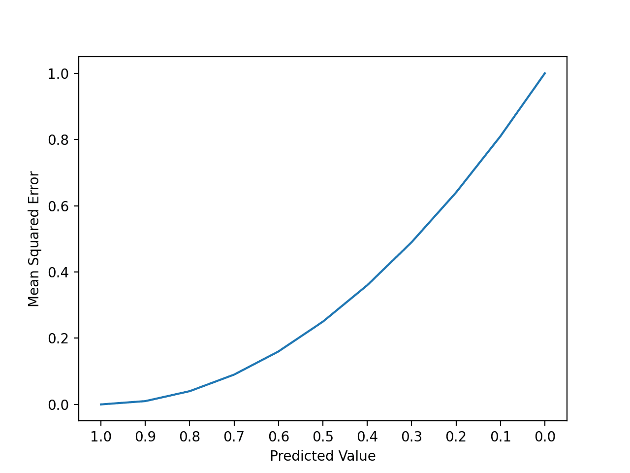
We can create a plot to get a feeling for how the change in prediction error impacts the squared error.
The example below gives a small contrived dataset of all 1.0 values and predictions that range from perfect (1.0) to wrong (0.0) by 0.1 increments. The squared error between each prediction and expected value is calculated and plotted to show the quadratic increase in squared error.
Running the example first reports the expected value, predicted value, and squared error for each case.
We can see that the error rises quickly, faster than linear (a straight line).
1
2
3
4
5
6
7
8
9
10
11
>1.0, 1.0 = 0.000
>1.0, 0.9 = 0.010
>1.0, 0.8 = 0.040
>1.0, 0.7 = 0.090
>1.0, 0.6 = 0.160
>1.0, 0.5 = 0.250
>1.0, 0.4 = 0.360
>1.0, 0.3 = 0.490
>1.0, 0.2 = 0.640
>1.0, 0.1 = 0.810
>1.0, 0.0 = 1.000
A line plot is created showing the curved or super-linear increase in the squared error value as the difference between the expected and predicted value is increased.
The curve is not a straight line as we might naively assume for an error metric.
Line Plot of the Increase Square Error With Predictions
The individual error terms are averaged so that we can report the performance of a model with regard to how much error the model makes generally when making predictions, rather than specifically for a given example.
The units of the MSE are squared units.
For example, if your target value represents “dollars,” then the MSE will be “squared dollars.” This can be confusing for stakeholders; therefore, when reporting results, often the root mean squared error is used instead (discussed in the next section).
The mean squared error between your expected and predicted values can be calculated using the mean_squared_error() function from the scikit-learn library.
The function takes a one-dimensional array or list of expected values and predicted values and returns the mean squared error value.
1
2
3
...
# calculate errors
errors=mean_squared_error(expected,predicted)
The example below gives an example of calculating the mean squared error between a list of contrived expected and predicted values.
Running the example calculates and prints the mean squared error.
1
0.35000000000000003
A perfect mean squared error value is 0.0, which means that all predictions matched the expected values exactly.
This is almost never the case, and if it happens, it suggests your predictive modeling problem is trivial.
A good MSE is relative to your specific dataset.
It is a good idea to first establish a baseline MSE for your dataset using a naive predictive model, such as predicting the mean target value from the training dataset. A model that achieves an MSE better than the MSE for the naive model has skill.
Importantly, the square root of the error is calculated, which means that the units of the RMSE are the same as the original units of the target value that is being predicted.
For example, if your target variable has the units “dollars,” then the RMSE error score will also have the unit “dollars” and not “squared dollars” like the MSE.
As such, it may be common to use MSE loss to train a regression predictive model, and to use RMSE to evaluate and report its performance.
The RMSE can be calculated as follows:
RMSE = sqrt(1 / N * sum for i to N (y_i – yhat_i)^2)
Where y_i is the i’th expected value in the dataset, yhat_i is the i’th predicted value, and sqrt() is the square root function.
We can restate the RMSE in terms of the MSE as:
RMSE = sqrt(MSE)
Note that the RMSE cannot be calculated as the average of the square root of the mean squared error values. This is a common error made by beginners and is an example of Jensen’s inequality.
You may recall that the square root is the inverse of the square operation. MSE uses the square operation to remove the sign of each error value and to punish large errors. The square root reverses this operation, although it ensures that the result remains positive.
The root mean squared error between your expected and predicted values can be calculated using the mean_squared_error() function from the scikit-learn library.
By default, the function calculates the MSE, but we can configure it to calculate the square root of the MSE by setting the “squared” argument to False.
The function takes a one-dimensional array or list of expected values and predicted values and returns the mean squared error value.
Running the example calculates and prints the root mean squared error.
1
0.5916079783099616
A perfect RMSE value is 0.0, which means that all predictions matched the expected values exactly.
This is almost never the case, and if it happens, it suggests your predictive modeling problem is trivial.
A good RMSE is relative to your specific dataset.
It is a good idea to first establish a baseline RMSE for your dataset using a naive predictive model, such as predicting the mean target value from the training dataset. A model that achieves an RMSE better than the RMSE for the naive model has skill.
Mean Absolute Error
Mean Absolute Error, or MAE, is a popular metric because, like RMSE, the units of the error score match the units of the target value that is being predicted.
Unlike the RMSE, the changes in MAE are linear and therefore intuitive.
That is, MSE and RMSE punish larger errors more than smaller errors, inflating or magnifying the mean error score. This is due to the square of the error value. The MAE does not give more or less weight to different types of errors and instead the scores increase linearly with increases in error.
As its name suggests, the MAE score is calculated as the average of the absolute error values. Absolute or abs() is a mathematical function that simply makes a number positive. Therefore, the difference between an expected and predicted value may be positive or negative and is forced to be positive when calculating the MAE.
The MAE can be calculated as follows:
MAE = 1 / N * sum for i to N abs(y_i – yhat_i)
Where y_i is the i’th expected value in the dataset, yhat_i is the i’th predicted value and abs() is the absolute function.
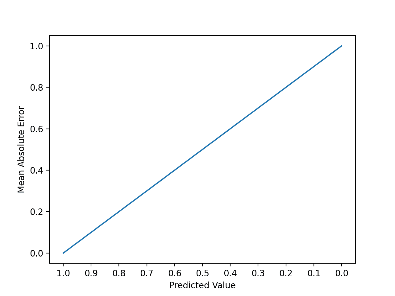
We can create a plot to get a feeling for how the change in prediction error impacts the MAE.
The example below gives a small contrived dataset of all 1.0 values and predictions that range from perfect (1.0) to wrong (0.0) by 0.1 increments. The absolute error between each prediction and expected value is calculated and plotted to show the linear increase in error.
1
2
3
...
# calculate error
err=abs((expected[i]-predicted[i]))
The complete example is listed below.
1
2
3
4
5
6
7
8
9
10
11
12
13
14
15
16
17
18
19
20
21
22
# plot of the increase of mean absolute error with prediction error
Running the example first reports the expected value, predicted value, and absolute error for each case.
We can see that the error rises linearly, which is intuitive and easy to understand.
1
2
3
4
5
6
7
8
9
10
11
>1.0, 1.0 = 0.000
>1.0, 0.9 = 0.100
>1.0, 0.8 = 0.200
>1.0, 0.7 = 0.300
>1.0, 0.6 = 0.400
>1.0, 0.5 = 0.500
>1.0, 0.4 = 0.600
>1.0, 0.3 = 0.700
>1.0, 0.2 = 0.800
>1.0, 0.1 = 0.900
>1.0, 0.0 = 1.000
A line plot is created showing the straight line or linear increase in the absolute error value as the difference between the expected and predicted value is increased.
Line Plot of the Increase Absolute Error With Predictions
The mean absolute error between your expected and predicted values can be calculated using the mean_absolute_error() function from the scikit-learn library.
The function takes a one-dimensional array or list of expected values and predicted values and returns the mean absolute error value.
1
2
3
...
# calculate errors
errors=mean_absolute_error(expected,predicted)
The example below gives an example of calculating the mean absolute error between a list of contrived expected and predicted values.
Running the example calculates and prints the mean absolute error.
1
0.5
A perfect mean absolute error value is 0.0, which means that all predictions matched the expected values exactly.
This is almost never the case, and if it happens, it suggests your predictive modeling problem is trivial.
A good MAE is relative to your specific dataset.
It is a good idea to first establish a baseline MAE for your dataset using a naive predictive model, such as predicting the mean target value from the training dataset. A model that achieves a MAE better than the MAE for the naive model has skill.
Further Reading
This section provides more resources on the topic if you are looking to go deeper.
Thank you so much for your great post. Do you have a plan to explain the other regression matrics, such as r2_score, RMSLE, MAPE, pearson correlation, and so on?
One thing that everyone is missing on MSE is that it punishing for large errors ONLY when the error is greater than 1. But in case of error in range from 0 to 1 (like in your case), taking square is actually discounting the error and we can see this clearly on your plot, where the straight line is actually ABOVE the MSE curve.
PD: is there any reason why you don’t use mathjax? it’s a javascript lib that let you display math formulas nicely, it would greatly improve readability.
Hi Jason,
great overview. I think there is a typo in this sentence at the start of the MAE section: “Unlike the RMSE, the changes in RMSE are linear and therefore intuitive.” Should it not read: “Unlike the RMSE, the changes in MAE are linear and therefore intuitive.”?
Hi. Thanks for the great article, it really helped! One question:
> It is a good idea to first establish a baseline MAE for your dataset using a naive predictive model, such as predicting the mean target value from the training dataset. A model that achieves a MAE better than the MAE for the naive model has skill.
How would one go about making a naive predictive model? By making a column for average target values and then predicting over it? Am I getting it right?
Hi Jason, can you please elaborate on this? How do I make a naive predictive model? I am embarrassed to admit, I am unable to understand what you mean with the average value from the training set.
Also, what is a ‘test harness’? In one XGBoost regression example you mention:
“Using a test harness of repeated stratified 10-fold cross-validation with three repeats, a naive model can achieve a mean absolute error (MAE) of about 6.6. A top-performing model can achieve a MAE on this same test harness of about 1.9. This provides the bounds of expected performance on this dataset.”
How does one find the naive model value and a top-performing model bounds? Thank you very much in advance.
Test harness just mean your suite of tests to be applied on a model. That supposed to be test cases of enough variation to give a good score to a model. In the quoted sentence, it is generated by stratified cross validation.
Thank you Adrian for your response. I understand what you mean.
I also later found this post where Jason explains how one does naive baseline predictions using Zero Rule Algorithm:
I know you didn’t discuss MAPE here, but you did mention the fact that we cannot calculate accuracy for a regression model. Do you have thoughts on subtracting MAPE from 1 to get an “accuracy” for reporting purposes?
Is it possible to set a target value for a machine learning model to reach? Say the model can produce an MAE of 0.7 but I want my MAE to be 0.2 and so I want the model to keep looping until it reaches the required value.
Is it possible, or is it just about accepting how the model can perform on the dataset?
Hey Jason, I’m a bit confused. In the Regression Predictive Modeling section you mention that “A problem with multiple input variables is often called a *multivariate regression* problem.”
But from what I’ve seen online elsewhere, multivariate regression problems are those with multiple output variables (ie. several y-variables). Whereas multiple regression problems are those with multiple input variables.
> A common question by beginners to regression predictive modeling projects is:
>
> How do I calculate accuracy for my regression model?
>
> Accuracy (e.g. classification accuracy) is a measure for classification, not regression.
>
> We cannot calculate accuracy for a regression model.
This is exactly the answer to the problem I am facing right now.
Many people still believe in deep learning and want accuracy anyway (despite the regression problem).
Indeed, metrics for regression problems, such as the ones described here, may be hard to imagine (for adults who have avoided learning mathematics).
I wonder if it would be better for them to understand the explanation given here, or if it would be better to show the Confusion Matrix, attributing it to a classification problem.
iPad is really not a very good environment for these things. If you get a bluetooth keyboard for it, probably you can simply use it as a browser and do your project on Google Colab.
Great article about the metrics but my small question is which is the correct formula for absolute error, is it actual values minus predicted values or predicted minus actual values
I have a question on evaluating the MSE for one step forecasting and multiple stoe forecasting.
the model is trained in two different way:
1. to perform one step forecasting with 60 time step of past values.
2. to perform 5 steps ahead forecasting with 60 time step of past values.
My question is whether multiple step ahead forecasting will improve the accuracy of first prediction or not?
For example,
I have trained one step forecasting and obtain the MSE of 0.045.
I also trained 5 steps ahead forecasting, but I calculated MSE for the one step ahead forecasting and I got MSE of 0.0047.
I tried to compare the MSE of one step ahead forecast for both model.
My hypothesis is, if we train a model with multiple steps ahead forecast will improve the accuracy of one step forecast. But the MSE didn’t show any improvement.
May I know is my hypothesis correct? Is model trained withmultiple step ahead forecasting will improve the accuracy of the one step ahead accuracy compare to model train with one step ahead forecasting?
You hypothesis may not always correct – it depends on the actual model. Consider the simplest ARIMA model with p=1, forecasting multiple steps ahead is just predicting noise.
I am trying to find the optimal input parameters so that the simulation model accurately predicts low and high values, i.e., the predicted values should be close to the 1:1 line (observed vs predicted). What would be the best error metrics in this case?
Hi,
It’s a really good article about the metrics in Regression. Thank you for this.
One common question like what is meant by “Robust to outliers”?. Can you please explain this terminology!
Hi Dafrin…this means that the model accuracy is not greatly affected by a relatively few data points that are not within the range of the majority of the data. More information can be found here:
Hello Jason. Very good article! I would like to ask. Can R squared be included as a metric of measuring the performance of a regression model? I would like to hear your opinion!


Thank you so much for your great post. Do you have a plan to explain the other regression matrics, such as r2_score, RMSLE, MAPE, pearson correlation, and so on?
Yes, I hope to in the future.
That would be great! 😉
This is nice, but the error of a straight line is above the parabola for values < 1, idk if that's an error or am I missing something probably?
Sorry I don’t follow, can you please elaborate?
One thing that everyone is missing on MSE is that it punishing for large errors ONLY when the error is greater than 1. But in case of error in range from 0 to 1 (like in your case), taking square is actually discounting the error and we can see this clearly on your plot, where the straight line is actually ABOVE the MSE curve.
You’re right. However, as a metric, it may not be an issue because values closer to 0 is discounted much more than those close to 1.
PD: is there any reason why you don’t use mathjax? it’s a javascript lib that let you display math formulas nicely, it would greatly improve readability.
But the post is great anyways!
Yes, it is intentional to make the content more approachable by developers.
Something interesting about MSE, is that if you have outliers, it will normally affect the errors and the algorithm quite a bit (imho).
Agreed, more punishment for the error in the outlier’s prediction.
Hi Jason,
great overview. I think there is a typo in this sentence at the start of the MAE section: “Unlike the RMSE, the changes in RMSE are linear and therefore intuitive.” Should it not read: “Unlike the RMSE, the changes in MAE are linear and therefore intuitive.”?
Thanks, fixed!
Hi. Thanks for the great article, it really helped! One question:
> It is a good idea to first establish a baseline MAE for your dataset using a naive predictive model, such as predicting the mean target value from the training dataset. A model that achieves a MAE better than the MAE for the naive model has skill.
How would one go about making a naive predictive model? By making a column for average target values and then predicting over it? Am I getting it right?
Yes!
You can predict the average value from the training set.
Hi Jason, can you please elaborate on this? How do I make a naive predictive model? I am embarrassed to admit, I am unable to understand what you mean with the average value from the training set.
Also, what is a ‘test harness’? In one XGBoost regression example you mention:
“Using a test harness of repeated stratified 10-fold cross-validation with three repeats, a naive model can achieve a mean absolute error (MAE) of about 6.6. A top-performing model can achieve a MAE on this same test harness of about 1.9. This provides the bounds of expected performance on this dataset.”
How does one find the naive model value and a top-performing model bounds? Thank you very much in advance.
Test harness just mean your suite of tests to be applied on a model. That supposed to be test cases of enough variation to give a good score to a model. In the quoted sentence, it is generated by stratified cross validation.
Thank you Adrian for your response. I understand what you mean.
I also later found this post where Jason explains how one does naive baseline predictions using Zero Rule Algorithm:
https://machinelearningmastery.com/implement-baseline-machine-learning-algorithms-scratch-python/
But I still don’t know how one can determine the upper bound for the expected performance on any given dataset. Thanks in advance everyone.
I know you didn’t discuss MAPE here, but you did mention the fact that we cannot calculate accuracy for a regression model. Do you have thoughts on subtracting MAPE from 1 to get an “accuracy” for reporting purposes?
It would be inverse MAPE (or something), not accuracy.
Hey there Jason.
Is it possible to set a target value for a machine learning model to reach? Say the model can produce an MAE of 0.7 but I want my MAE to be 0.2 and so I want the model to keep looping until it reaches the required value.
Is it possible, or is it just about accepting how the model can perform on the dataset?
It may not be possible to achieve a given metric score for a given model + dataset + test test harness.
Hey Jason, I’m a bit confused. In the Regression Predictive Modeling section you mention that “A problem with multiple input variables is often called a *multivariate regression* problem.”
But from what I’ve seen online elsewhere, multivariate regression problems are those with multiple output variables (ie. several y-variables). Whereas multiple regression problems are those with multiple input variables.
For example:
https://www.quora.com/What-is-the-difference-between-a-multiple-linear-regression-and-a-multivariate-regression
Perhaps this may help:
https://machinelearningmastery.com/taxonomy-of-time-series-forecasting-problems/
At the end of the day, use terms that help you understand your problem.
Thank you so much for your great post.
> A common question by beginners to regression predictive modeling projects is:
>
> How do I calculate accuracy for my regression model?
>
> Accuracy (e.g. classification accuracy) is a measure for classification, not regression.
>
> We cannot calculate accuracy for a regression model.
This is exactly the answer to the problem I am facing right now.
Many people still believe in deep learning and want accuracy anyway (despite the regression problem).
Indeed, metrics for regression problems, such as the ones described here, may be hard to imagine (for adults who have avoided learning mathematics).
I wonder if it would be better for them to understand the explanation given here, or if it would be better to show the Confusion Matrix, attributing it to a classification problem.
I’m happy to hear that the tutorial was helpful.
At least, I’m learning……………………
That’s great!
Hello, I was just wondering if you know any software that I can use on my iPad, if there’s any. Thanks.
iPad is really not a very good environment for these things. If you get a bluetooth keyboard for it, probably you can simply use it as a browser and do your project on Google Colab.
Great article about the metrics but my small question is which is the correct formula for absolute error, is it actual values minus predicted values or predicted minus actual values
Doesn’t matter – because you’ll take the absolute value of the difference.
Hi Jason,
I have a question on evaluating the MSE for one step forecasting and multiple stoe forecasting.
the model is trained in two different way:
1. to perform one step forecasting with 60 time step of past values.
2. to perform 5 steps ahead forecasting with 60 time step of past values.
My question is whether multiple step ahead forecasting will improve the accuracy of first prediction or not?
For example,
I have trained one step forecasting and obtain the MSE of 0.045.
I also trained 5 steps ahead forecasting, but I calculated MSE for the one step ahead forecasting and I got MSE of 0.0047.
I tried to compare the MSE of one step ahead forecast for both model.
My hypothesis is, if we train a model with multiple steps ahead forecast will improve the accuracy of one step forecast. But the MSE didn’t show any improvement.
May I know is my hypothesis correct? Is model trained withmultiple step ahead forecasting will improve the accuracy of the one step ahead accuracy compare to model train with one step ahead forecasting?
Thank you very much
You hypothesis may not always correct – it depends on the actual model. Consider the simplest ARIMA model with p=1, forecasting multiple steps ahead is just predicting noise.
Thanks for the great article.
Is there a metric for choosing which of the several effectiveness indicators to use?
I just found the following article very helpful on the issue of classification.
https://machinelearningmastery.com/tour-of-evaluation-metrics-for-imbalanced-classification/
Best regards.
I am trying to find the optimal input parameters so that the simulation model accurately predicts low and high values, i.e., the predicted values should be close to the 1:1 line (observed vs predicted). What would be the best error metrics in this case?
Hi Urs…You may find the following helpful:
https://machinelearningmastery.com/optimization-for-machine-learning-crash-course/
Hi,
It’s a really good article about the metrics in Regression. Thank you for this.
One common question like what is meant by “Robust to outliers”?. Can you please explain this terminology!
Hi Dafrin…this means that the model accuracy is not greatly affected by a relatively few data points that are not within the range of the majority of the data. More information can be found here:
https://machinelearningmastery.com/robust-regression-for-machine-learning-in-python/
Hello Jason. Very good article! I would like to ask. Can R squared be included as a metric of measuring the performance of a regression model? I would like to hear your opinion!
You are very welcome Kostas! The following may be of interest to you:
https://www.statology.org/r-squared-in-python/
What is R2 ?
Is it different from the three error metrics defined in the article ?
1)MSE
2)RMSE
3)MAE
Please elaborate .
Hi Sandeep…The following resource may add clarity:
https://statisticsbyjim.com/regression/interpret-r-squared-regression/
Thanku so much for this tutorial,,, it helps alot… ????