From Developer to Machine Learning Practitioner in 14 Days
Python is one of the fastest-growing platforms for applied machine learning.
In this mini-course, you will discover how you can get started, build accurate models and confidently complete predictive modeling machine learning projects using Python in 14 days.
This is a big and important post. You might want to bookmark it.
Kick-start your project with my new book Machine Learning Mastery With Python, including step-by-step tutorials and the Python source code files for all examples.
Let’s get started.
- Update Oct/2016: Updated examples for sklearn v0.18.
- Update Feb/2018: Update Python and library versions.
- Update Mar/2018: Added alternate link to download some datasets.
- Update May/2019: Fixed warning messages for latest version of scikit-learn .
- Update Oct/2020: Updated broken link for Anaconda.

Python Machine Learning Mini-Course
Photo by Dave Young, some rights reserved.
Who Is This Mini-Course For?
Before we get started, let’s make sure you are in the right place.
The list below provides some general guidelines as to who this course was designed for.
Don’t panic if you don’t match these points exactly, you might just need to brush up in one area or another to keep up.
- Developers that know how to write a little code. This means that it is not a big deal for you to pick up a new programming language like Python once you know the basic syntax. It does not mean you’re a wizard coder, just that you can follow a basic C-like language with little effort.
- Developers that know a little machine learning. This means you know the basics of machine learning like cross-validation, some algorithms and the bias-variance trade-off. It does not mean that you are a machine learning Ph.D., just that you know the landmarks or know where to look them up.
This mini-course is neither a textbook on Python or a textbook on machine learning.
It will take you from a developer that knows a little machine learning to a developer who can get results using the Python ecosystem, the rising platform for professional machine learning.
Need help with Machine Learning in Python?
Take my free 2-week email course and discover data prep, algorithms and more (with code).
Click to sign-up now and also get a free PDF Ebook version of the course.
Mini-Course Overview
This mini-course is broken down into 14 lessons.
You could complete one lesson per day (recommended) or complete all of the lessons in one day (hard core!). It really depends on the time you have available and your level of enthusiasm.
Below are 14 lessons that will get you started and productive with machine learning in Python:
- Lesson 1: Download and Install Python and SciPy ecosystem.
- Lesson 2: Get Around In Python, NumPy, Matplotlib and Pandas.
- Lesson 3: Load Data From CSV.
- Lesson 4: Understand Data with Descriptive Statistics.
- Lesson 5: Understand Data with Visualization.
- Lesson 6: Prepare For Modeling by Pre-Processing Data.
- Lesson 7: Algorithm Evaluation With Resampling Methods.
- Lesson 8: Algorithm Evaluation Metrics.
- Lesson 9: Spot-Check Algorithms.
- Lesson 10: Model Comparison and Selection.
- Lesson 11: Improve Accuracy with Algorithm Tuning.
- Lesson 12: Improve Accuracy with Ensemble Predictions.
- Lesson 13: Finalize And Save Your Model.
- Lesson 14: Hello World End-to-End Project.
Each lesson could take you 60 seconds or up to 30 minutes. Take your time and complete the lessons at your own pace. Ask questions and even post results in the comments below.
The lessons expect you to go off and find out how to do things. I will give you hints, but part of the point of each lesson is to force you to learn where to go to look for help on and about the Python platform (hint, I have all of the answers directly on this blog, use the search feature).
I do provide more help in the early lessons because I want you to build up some confidence and inertia.
Hang in there, don’t give up!
Lesson 1: Download and Install Python and SciPy
You cannot get started with machine learning in Python until you have access to the platform.
Today’s lesson is easy, you must download and install the Python 3.6 platform on your computer.
Visit the Python homepage and download Python for your operating system (Linux, OS X or Windows). Install Python on your computer. You may need to use a platform specific package manager such as macports on OS X or yum on RedHat Linux.
You also need to install the SciPy platform and the scikit-learn library. I recommend using the same approach that you used to install Python.
You can install everything at once (much easier) with Anaconda. Recommended for beginners.
Start Python for the first time by typing “python” at the command line.
Check the versions of everything you are going to need using the code below:
|
1 2 3 4 5 6 7 8 9 10 11 12 13 14 15 16 17 18 |
# Python version import sys print('Python: {}'.format(sys.version)) # scipy import scipy print('scipy: {}'.format(scipy.__version__)) # numpy import numpy print('numpy: {}'.format(numpy.__version__)) # matplotlib import matplotlib print('matplotlib: {}'.format(matplotlib.__version__)) # pandas import pandas print('pandas: {}'.format(pandas.__version__)) # scikit-learn import sklearn print('sklearn: {}'.format(sklearn.__version__)) |
If there are any errors, stop. Now is the time to fix them.
Need help? See this tutorial:
Lesson 2: Get Around In Python, NumPy, Matplotlib and Pandas.
You need to be able to read and write basic Python scripts.
As a developer, you can pick-up new programming languages pretty quickly. Python is case sensitive, uses hash (#) for comments and uses whitespace to indicate code blocks (whitespace matters).
Today’s task is to practice the basic syntax of the Python programming language and important SciPy data structures in the Python interactive environment.
- Practice assignment, working with lists and flow control in Python.
- Practice working with NumPy arrays.
- Practice creating simple plots in Matplotlib.
- Practice working with Pandas Series and DataFrames.
For example, below is a simple example of creating a Pandas DataFrame.
|
1 2 3 4 5 6 7 8 |
# dataframe import numpy import pandas myarray = numpy.array([[1, 2, 3], [4, 5, 6]]) rownames = ['a', 'b'] colnames = ['one', 'two', 'three'] mydataframe = pandas.DataFrame(myarray, index=rownames, columns=colnames) print(mydataframe) |
Lesson 3: Load Data From CSV
Machine learning algorithms need data. You can load your own data from CSV files but when you are getting started with machine learning in Python you should practice on standard machine learning datasets.
Your task for today’s lesson is to get comfortable loading data into Python and to find and load standard machine learning datasets.
There are many excellent standard machine learning datasets in CSV format that you can download and practice with on the UCI machine learning repository.
- Practice loading CSV files into Python using the CSV.reader() in the standard library.
- Practice loading CSV files using NumPy and the numpy.loadtxt() function.
- Practice loading CSV files using Pandas and the pandas.read_csv() function.
To get you started, below is a snippet that will load the Pima Indians onset of diabetes dataset using Pandas directly from the UCI Machine Learning Repository.
|
1 2 3 4 5 6 |
# Load CSV using Pandas from URL import pandas url = "https://raw.githubusercontent.com/jbrownlee/Datasets/master/pima-indians-diabetes.data.csv" names = ['preg', 'plas', 'pres', 'skin', 'test', 'mass', 'pedi', 'age', 'class'] data = pandas.read_csv(url, names=names) print(data.shape) |
Well done for making it this far! Hang in there.
Any questions so far? Ask in the comments.
Lesson 4: Understand Data with Descriptive Statistics
Once you have loaded your data into Python you need to be able to understand it.
The better you can understand your data, the better and more accurate the models that you can build. The first step to understanding your data is to use descriptive statistics.
Today your lesson is to learn how to use descriptive statistics to understand your data. I recommend using the helper functions provided on the Pandas DataFrame.
- Understand your data using the head() function to look at the first few rows.
- Review the dimensions of your data with the shape property.
- Look at the data types for each attribute with the dtypes property.
- Review the distribution of your data with the describe() function.
- Calculate pairwise correlation between your variables using the corr() function.
The below example loads the Pima Indians onset of diabetes dataset and summarizes the distribution of each attribute.
|
1 2 3 4 5 6 7 |
# Statistical Summary import pandas url = "https://raw.githubusercontent.com/jbrownlee/Datasets/master/pima-indians-diabetes.data.csv" names = ['preg', 'plas', 'pres', 'skin', 'test', 'mass', 'pedi', 'age', 'class'] data = pandas.read_csv(url, names=names) description = data.describe() print(description) |
Try it out!
Lesson 5: Understand Data with Visualization
Continuing on from yesterday’s lesson, you must spend time to better understand your data.
A second way to improve your understanding of your data is by using data visualization techniques (e.g. plotting).
Today, your lesson is to learn how to use plotting in Python to understand attributes alone and their interactions. Again, I recommend using the helper functions provided on the Pandas DataFrame.
- Use the hist() function to create a histogram of each attribute.
- Use the plot(kind=’box’) function to create box-and-whisker plots of each attribute.
- Use the pandas.scatter_matrix() function to create pairwise scatterplots of all attributes.
For example, the snippet below will load the diabetes dataset and create a scatterplot matrix of the dataset.
|
1 2 3 4 5 6 7 8 9 |
# Scatter Plot Matrix import matplotlib.pyplot as plt import pandas from pandas.plotting import scatter_matrix url = "https://raw.githubusercontent.com/jbrownlee/Datasets/master/pima-indians-diabetes.data.csv" names = ['preg', 'plas', 'pres', 'skin', 'test', 'mass', 'pedi', 'age', 'class'] data = pandas.read_csv(url, names=names) scatter_matrix(data) plt.show() |
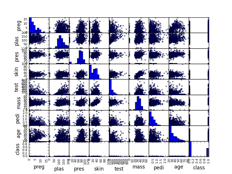
Sample Scatter Plot Matrix
Lesson 6: Prepare For Modeling by Pre-Processing Data
Your raw data may not be setup to be in the best shape for modeling.
Sometimes you need to preprocess your data in order to best present the inherent structure of the problem in your data to the modeling algorithms. In today’s lesson, you will use the pre-processing capabilities provided by the scikit-learn.
The scikit-learn library provides two standard idioms for transforming data. Each transform is useful in different circumstances: Fit and Multiple Transform and Combined Fit-And-Transform.
There are many techniques that you can use to prepare your data for modeling. For example, try out some of the following
- Standardize numerical data (e.g. mean of 0 and standard deviation of 1) using the scale and center options.
- Normalize numerical data (e.g. to a range of 0-1) using the range option.
- Explore more advanced feature engineering such as Binarizing.
For example, the snippet below loads the Pima Indians onset of diabetes dataset, calculates the parameters needed to standardize the data, then creates a standardized copy of the input data.
|
1 2 3 4 5 6 7 8 9 10 11 12 13 14 15 16 |
# Standardize data (0 mean, 1 stdev) from sklearn.preprocessing import StandardScaler import pandas import numpy url = "https://raw.githubusercontent.com/jbrownlee/Datasets/master/pima-indians-diabetes.data.csv" names = ['preg', 'plas', 'pres', 'skin', 'test', 'mass', 'pedi', 'age', 'class'] dataframe = pandas.read_csv(url, names=names) array = dataframe.values # separate array into input and output components X = array[:,0:8] Y = array[:,8] scaler = StandardScaler().fit(X) rescaledX = scaler.transform(X) # summarize transformed data numpy.set_printoptions(precision=3) print(rescaledX[0:5,:]) |
Lesson 7: Algorithm Evaluation With Resampling Methods
The dataset used to train a machine learning algorithm is called a training dataset. The dataset used to train an algorithm cannot be used to give you reliable estimates of the accuracy of the model on new data. This is a big problem because the whole idea of creating the model is to make predictions on new data.
You can use statistical methods called resampling methods to split your training dataset up into subsets, some are used to train the model and others are held back and used to estimate the accuracy of the model on unseen data.
Your goal with today’s lesson is to practice using the different resampling methods available in scikit-learn, for example:
- Split a dataset into training and test sets.
- Estimate the accuracy of an algorithm using k-fold cross validation.
- Estimate the accuracy of an algorithm using leave one out cross validation.
The snippet below uses scikit-learn to estimate the accuracy of the Logistic Regression algorithm on the Pima Indians onset of diabetes dataset using 10-fold cross validation.
|
1 2 3 4 5 6 7 8 9 10 11 12 13 14 15 |
# Evaluate using Cross Validation from pandas import read_csv from sklearn.model_selection import KFold from sklearn.model_selection import cross_val_score from sklearn.linear_model import LogisticRegression url = "https://raw.githubusercontent.com/jbrownlee/Datasets/master/pima-indians-diabetes.data.csv" names = ['preg', 'plas', 'pres', 'skin', 'test', 'mass', 'pedi', 'age', 'class'] dataframe = read_csv(url, names=names) array = dataframe.values X = array[:,0:8] Y = array[:,8] kfold = KFold(n_splits=10, random_state=7, shuffle=True) model = LogisticRegression(solver='liblinear') results = cross_val_score(model, X, Y, cv=kfold) print("Accuracy: %.3f%% (%.3f%%)" % (results.mean()*100.0, results.std()*100.0)) |
What accuracy did you get? Let me know in the comments.
Did you realize that this is the halfway point? Well done!
Lesson 8: Algorithm Evaluation Metrics
There are many different metrics that you can use to evaluate the skill of a machine learning algorithm on a dataset.
You can specify the metric used for your test harness in scikit-learn via the cross_validation.cross_val_score() function and defaults can be used for regression and classification problems. Your goal with today’s lesson is to practice using the different algorithm performance metrics available in the scikit-learn package.
- Practice using the Accuracy and LogLoss metrics on a classification problem.
- Practice generating a confusion matrix and a classification report.
- Practice using RMSE and RSquared metrics on a regression problem.
The snippet below demonstrates calculating the LogLoss metric on the Pima Indians onset of diabetes dataset.
|
1 2 3 4 5 6 7 8 9 10 11 12 13 14 15 16 |
# Cross Validation Classification LogLoss from pandas import read_csv from sklearn.model_selection import KFold from sklearn.model_selection import cross_val_score from sklearn.linear_model import LogisticRegression url = "https://raw.githubusercontent.com/jbrownlee/Datasets/master/pima-indians-diabetes.data.csv" names = ['preg', 'plas', 'pres', 'skin', 'test', 'mass', 'pedi', 'age', 'class'] dataframe = read_csv(url, names=names) array = dataframe.values X = array[:,0:8] Y = array[:,8] kfold = KFold(n_splits=10, random_state=7) model = LogisticRegression(solver='liblinear') scoring = 'neg_log_loss' results = cross_val_score(model, X, Y, cv=kfold, scoring=scoring) print("Logloss: %.3f (%.3f)") % (results.mean(), results.std()) |
What log loss did you get? Let me know in the comments.
Lesson 9: Spot-Check Algorithms
You cannot possibly know which algorithm will perform best on your data beforehand.
You have to discover it using a process of trial and error. I call this spot-checking algorithms. The scikit-learn library provides an interface to many machine learning algorithms and tools to compare the estimated accuracy of those algorithms.
In this lesson, you must practice spot checking different machine learning algorithms.
- Spot check linear algorithms on a dataset (e.g. linear regression, logistic regression and linear discriminate analysis).
- Spot check some non-linear algorithms on a dataset (e.g. KNN, SVM and CART).
- Spot-check some sophisticated ensemble algorithms on a dataset (e.g. random forest and stochastic gradient boosting).
For example, the snippet below spot-checks the K-Nearest Neighbors algorithm on the Boston House Price dataset.
|
1 2 3 4 5 6 7 8 9 10 11 12 13 14 15 16 |
# KNN Regression from pandas import read_csv from sklearn.model_selection import KFold from sklearn.model_selection import cross_val_score from sklearn.neighbors import KNeighborsRegressor url = "https://raw.githubusercontent.com/jbrownlee/Datasets/master/housing.data" names = ['CRIM', 'ZN', 'INDUS', 'CHAS', 'NOX', 'RM', 'AGE', 'DIS', 'RAD', 'TAX', 'PTRATIO', 'B', 'LSTAT', 'MEDV'] dataframe = read_csv(url, delim_whitespace=True, names=names) array = dataframe.values X = array[:,0:13] Y = array[:,13] kfold = KFold(n_splits=10, random_state=7) model = KNeighborsRegressor() scoring = 'neg_mean_squared_error' results = cross_val_score(model, X, Y, cv=kfold, scoring=scoring) print(results.mean()) |
What mean squared error did you get? Let me know in the comments.
Lesson 10: Model Comparison and Selection
Now that you know how to spot check machine learning algorithms on your dataset, you need to know how to compare the estimated performance of different algorithms and select the best model.
In today’s lesson, you will practice comparing the accuracy of machine learning algorithms in Python with scikit-learn.
- Compare linear algorithms to each other on a dataset.
- Compare nonlinear algorithms to each other on a dataset.
- Compare different configurations of the same algorithm to each other.
- Create plots of the results comparing algorithms.
The example below compares Logistic Regression and Linear Discriminant Analysis to each other on the Pima Indians onset of diabetes dataset.
|
1 2 3 4 5 6 7 8 9 10 11 12 13 14 15 16 17 18 19 20 21 22 23 24 25 26 27 28 |
# Compare Algorithms from pandas import read_csv from sklearn.model_selection import KFold from sklearn.model_selection import cross_val_score from sklearn.linear_model import LogisticRegression from sklearn.discriminant_analysis import LinearDiscriminantAnalysis # load dataset url = "https://raw.githubusercontent.com/jbrownlee/Datasets/master/pima-indians-diabetes.data.csv" names = ['preg', 'plas', 'pres', 'skin', 'test', 'mass', 'pedi', 'age', 'class'] dataframe = read_csv(url, names=names) array = dataframe.values X = array[:,0:8] Y = array[:,8] # prepare models models = [] models.append(('LR', LogisticRegression(solver='liblinear'))) models.append(('LDA', LinearDiscriminantAnalysis())) # evaluate each model in turn results = [] names = [] scoring = 'accuracy' for name, model in models: kfold = KFold(n_splits=10, random_state=7) cv_results = cross_val_score(model, X, Y, cv=kfold, scoring=scoring) results.append(cv_results) names.append(name) msg = "%s: %f (%f)" % (name, cv_results.mean(), cv_results.std()) print(msg) |
Which algorithm got better results? Can you do better? Let me know in the comments.
Lesson 11: Improve Accuracy with Algorithm Tuning
Once you have found one or two algorithms that perform well on your dataset, you may want to improve the performance of those models.
One way to increase the performance of an algorithm is to tune its parameters to your specific dataset.
The scikit-learn library provides two ways to search for combinations of parameters for a machine learning algorithm. Your goal in today’s lesson is to practice each.
- Tune the parameters of an algorithm using a grid search that you specify.
- Tune the parameters of an algorithm using a random search.
The snippet below uses is an example of using a grid search for the Ridge Regression algorithm on the Pima Indians onset of diabetes dataset.
|
1 2 3 4 5 6 7 8 9 10 11 12 13 14 15 16 17 18 |
# Grid Search for Algorithm Tuning from pandas import read_csv import numpy from sklearn.linear_model import Ridge from sklearn.model_selection import GridSearchCV url = "https://raw.githubusercontent.com/jbrownlee/Datasets/master/pima-indians-diabetes.data.csv" names = ['preg', 'plas', 'pres', 'skin', 'test', 'mass', 'pedi', 'age', 'class'] dataframe = read_csv(url, names=names) array = dataframe.values X = array[:,0:8] Y = array[:,8] alphas = numpy.array([1,0.1,0.01,0.001,0.0001,0]) param_grid = dict(alpha=alphas) model = Ridge() grid = GridSearchCV(estimator=model, param_grid=param_grid, cv=3) grid.fit(X, Y) print(grid.best_score_) print(grid.best_estimator_.alpha) |
Which parameters achieved the best results? Can you do better? Let me know in the comments.
Lesson 12: Improve Accuracy with Ensemble Predictions
Another way that you can improve the performance of your models is to combine the predictions from multiple models.
Some models provide this capability built-in such as random forest for bagging and stochastic gradient boosting for boosting. Another type of ensembling called voting can be used to combine the predictions from multiple different models together.
In today’s lesson, you will practice using ensemble methods.
- Practice bagging ensembles with the random forest and extra trees algorithms.
- Practice boosting ensembles with the gradient boosting machine and AdaBoost algorithms.
- Practice voting ensembles using by combining the predictions from multiple models together.
The snippet below demonstrates how you can use the Random Forest algorithm (a bagged ensemble of decision trees) on the Pima Indians onset of diabetes dataset.
|
1 2 3 4 5 6 7 8 9 10 11 12 13 14 15 16 17 |
# Random Forest Classification from pandas import read_csv from sklearn.model_selection import KFold from sklearn.model_selection import cross_val_score from sklearn.ensemble import RandomForestClassifier url = "https://raw.githubusercontent.com/jbrownlee/Datasets/master/pima-indians-diabetes.data.csv" names = ['preg', 'plas', 'pres', 'skin', 'test', 'mass', 'pedi', 'age', 'class'] dataframe = read_csv(url, names=names) array = dataframe.values X = array[:,0:8] Y = array[:,8] num_trees = 100 max_features = 3 kfold = KFold(n_splits=10, random_state=7) model = RandomForestClassifier(n_estimators=num_trees, max_features=max_features) results = cross_val_score(model, X, Y, cv=kfold) print(results.mean()) |
Can you devise a better ensemble? Let me know in the comments.
Lesson 13: Finalize And Save Your Model
Once you have found a well-performing model on your machine learning problem, you need to finalize it.
In today’s lesson, you will practice the tasks related to finalizing your model.
Practice making predictions with your model on new data (data unseen during training and testing).
Practice saving trained models to file and loading them up again.
For example, the snippet below shows how you can create a Logistic Regression model, save it to file, then load it later and make predictions on unseen data.
|
1 2 3 4 5 6 7 8 9 10 11 12 13 14 15 16 17 18 19 20 21 22 23 24 25 26 27 |
# Save Model Using Pickle from pandas import read_csv from sklearn.model_selection import train_test_split from sklearn.linear_model import LogisticRegression import pickle url = "https://raw.githubusercontent.com/jbrownlee/Datasets/master/pima-indians-diabetes.data.csv" names = ['preg', 'plas', 'pres', 'skin', 'test', 'mass', 'pedi', 'age', 'class'] dataframe = read_csv(url, names=names) array = dataframe.values X = array[:,0:8] Y = array[:,8] test_size = 0.33 seed = 7 X_train, X_test, Y_train, Y_test = train_test_split(X, Y, test_size=test_size, random_state=seed) # Fit the model on 67% model = LogisticRegression(solver='liblinear') model.fit(X_train, Y_train) # save the model to disk filename = 'finalized_model.sav' pickle.dump(model, open(filename, 'wb')) # some time later... # load the model from disk loaded_model = pickle.load(open(filename, 'rb')) result = loaded_model.score(X_test, Y_test) print(result) |
Lesson 14: Hello World End-to-End Project
You now know how to complete each task of a predictive modeling machine learning problem.
In today’s lesson, you need to practice putting the pieces together and working through a standard machine learning dataset end-to-end.
Work through the iris dataset end-to-end (the hello world of machine learning)
This includes the steps:
- Understanding your data using descriptive statistics and visualization.
- Preprocessing the data to best expose the structure of the problem.
- Spot-checking a number of algorithms using your own test harness.
- Improving results using algorithm parameter tuning.
- Improving results using ensemble methods.
- Finalize the model ready for future use.
Take it slowly and record your results along the way.
What model did you use? What results did you get? Let me know in the comments.
The End!
(Look How Far You Have Come)
You made it. Well done!
Take a moment and look back at how far you have come.
- You started off with an interest in machine learning and a strong desire to be able to practice and apply machine learning using Python.
- You downloaded, installed and started Python, perhaps for the first time and started to get familiar with the syntax of the language.
- Slowly and steadily over the course of a number of lessons you learned how the standard tasks of a predictive modeling machine learning project map onto the Python platform.
- Building upon the recipes for common machine learning tasks you worked through your first machine learning problems end-to-end using Python.
- Using a standard template, the recipes and experience you have gathered you are now capable of working through new and different predictive modeling machine learning problems on your own.
Don’t make light of this, you have come a long way in a short amount of time.
This is just the beginning of your machine learning journey with Python. Keep practicing and developing your skills.
Summary
How Did You Go With The Mini-Course?
Did you enjoy this mini-course?
Do you have any questions? Were there any sticking points?
Let me know. Leave a comment below.
Discover Fast Machine Learning in Python!
Develop Your Own Models in Minutes
...with just a few lines of scikit-learn code
Learn how in my new Ebook:
Machine Learning Mastery With Python
Covers self-study tutorials and end-to-end projects like:
Loading data, visualization, modeling, tuning, and much more...
Finally Bring Machine Learning To
Your Own Projects
Skip the Academics. Just Results.


Accuracy: 76.951% (4.841%)
Nice work!
Please tell me what LogLoss really is in lesson 8?
You can learn more here:
https://en.wikipedia.org/wiki/Loss_functions_for_classification
This wikipedia material about loss function is too complicated for someone with non-mathematics background. Are there materials for dummies?
Yes, this might help:
https://machinelearningmastery.com/loss-and-loss-functions-for-training-deep-learning-neural-networks/
Hi Jason !
Thank you so much for these lessons. It got me started on Python very quickly. I’m currently in lesson 7. I tried LeaveOneOut resampling method and got: Accuracy: 76.823% (42.196%).
I have a question: how do we consider a model better than others: it seems accuracy is not enough, we should also consider lower variance in the cross validation, shouldn’t we?
Thanks!
Sarra
Great question.
A model is good relative to the skill of a baseline model on the problem, such as the Zero Rule algorithm.
Hello Jason,
Keep up the good work! Your lessons are extremely helpful !!
Just to check, I’m in lesson 9 and was wondering if my results look correct:
Nearest Neighbors – Negative mean squared error: -107.287
Support Vector Machine – Negative mean squared error: -91.048
Decision Tree – Negative mean squared error: -40.102
Linear Regression – Negative mean squared error: -34.705
Logistic Regression – Negative mean squared error: -40.419
Random Forest – Negative mean squared error: -22.546
Stochastic Gradient Boosting – Negative mean squared error: -18.711
Also, I have some issues on the LDA (error: Unknown label type). I read that it is a classifier, but since our output variable is not a class, we cannot use LDA in case of Boston Houses Prices dataset, am I right?
Thank you !
Nice work.
LDA cannot be used for regression, it is a classification algorithm.
Hi Jason,
First of all, thank you for your quick replies! As I progress towards the last lessons, I have always this question: what happens if we don’t specify a value for ‘scoring’ in cross_val_score? The documentation says default value is ‘None’, but then how can we interpret the value of results.meant() if no scoring is specified?
Thanks!
Sarra
Good question, I don’t know the default behavior. It might be accuracy/mse for classification/regression, but that is just a guess. I’d recommend specifying something.
Hi Jason,
Less12: What does max_feature stand for? Why did you choose 3 in your example?
model = RandomForestClassifier(n_estimators=num_trees, max_features=max_features)
Thanks!
Sarra
Hi Sarra, I chose 3 features arbitrary for the example.
Accuracy: 76.951% (4.841%)
in lesson 7 this work for me
accu = (“Accuracy: %.3f%% (%.3f%%)”) % (results.mean()*100.0, results.std()*100.0)
print(accu)
Thanks. I encountered the same problem.
Dominique
Lesson 7: Accuracy: 77.086% (5.091%)
Lesson 8: Logloss: -0.494 (0.042)
Lesson 9: mean: -38.85
Hi Jason. Thanks for ALL you do. I was doing “Lesson 7: Algorithm Evaluation With Resampling Methods”, when I ran into the following challenges running Python 35 with sklearn VERSION 0.18. :
c:\python35\lib\site-packages\sklearn\cross_validation.py:44: DeprecationWarning: This module was deprecated in version 0.18 in favor of the model_selection module into which all the refactored classes and functions are moved. Also note that the interface of the new CV iterators are different from that of this module. This module will be removed in 0.20.
“This module will be removed in 0.20.”, DeprecationWarning)
ALSO:
TypeError Traceback (most recent call last)
in ()
51 done results = cross_val_score
52 “””
—> 53 print(“Accuracy: %.3f%% (%.3f%%)”) % (results.mean()*100.0, results.std()*100.0)
TypeError: unsupported operand type(s) for %: ‘NoneType’ and ‘tuple’
Continuation of above reply:
Jason i think your print statement:
print(“Accuracy: %.3f%% (%.3f%%)”) % (results.mean()*100.0, results.std()*100.0)
should look like:
print(“Accuracy: %.3f (%.3f)” % (results.mean()*100.0, results.std()*100.0))
Thanks again for the GREAT info.
Love and peace,
Joe
Glad to hear you worked it out. Perhaps it was a Python 3 thing? The code works in Python 2.7
I will look at the Deprecation Warning ASAP.
Thanks for the reply, Jason.
Love and peace,
Joe
Doesn’t work for me on using Python 3:
print(“Accuracy: %.3f%% (%.3f%%)”) % (results.mean()*100.0, results.std()*100.0))
Had an extra ‘)’ which I removed:
print(“Accuracy: %.3f%% (%.3f%%)” % (results.mean()*100.0, results.std()*100.0))
Thanks! Fixed.
Hi Jason,
Here’s what i got for the log loss == ‘neg_log_loss’ scoring on the LogisticRegression Model
model: LogisticRegression – scoring: neg_lo_loss
– results summary: -49.255 mean (4.705) std
– sorted(results):
[-0.57565879615204196, -0.52778706048371593, -0.52755866512803806, -0.51792016214361636, -0.5127963295718494, -0.49019538734940965, -0.47043507959473152, -0.4514763172464305, -0.44345852864232038, -0.40816890220694385]
Thanks for the great work. I’ll take up your email course after i finish with this.
Love and peace,
Joe
Thanks Joe, nice work.
Dear Jason,
Regarding “Lesson 9: Spot-Check Algorithms”, I would like to know how can I use Data Preparation for various (Dataset, Model(Algorithm), Scoring) combinations, AND which (Dataset, Model(Algorithm), Scoring) combinations are JUST INCOMPATIBLE?
I have published a post on my blog titled “Naive Spot-Check of AI Algorithms” which references your work. The post generates 36 Spot-Check Cases, using (3 Datasets x 4 Models(Algorithms) x 3 Scorings). There were 11 out of 36 Cases that returned numerical results. The other 25 Cases returned Errors or Warnings.
Again, I would like to know how can I use Data Preparation for various (Dataset, Model(Algorithm), Scoring) combinations, AND which (Dataset, Model(Algorithm), Scoring) combinations are JUST INCOMPATIBLE?
Thanks for the GREAT work.
Love and peace,
Joe
Here’s the link to my post, “Naive Spot-Check of AI Algorithms”,
https://joecodeswell.wordpress.com/2016/10/28/naive-spot-check-of-ai-algorithms/
Thanks again, Jason.
Love and peace,
Joe
Nice post and great question Joe.
Spot checking is to discover which algorithms look good on one given dataset. Not across datasets.
You may need to group algorithms by their expectations then prepare data for each group.
Most machine learning algorithms expect data to have numeric input values and an integer encoded or one hot encoded output value for classification. This is a good normalized view of a dataset to construct.
Here’s a tutorial that shows how to spot check 7 machine learning algorithms on one problem in Python:
https://machinelearningmastery.com/spot-check-regression-machine-learning-algorithms-python-scikit-learn/
Hi Jason, thanks for the post. I’m running into issues while executing Lesson 7
from sklearn.model_selection import KFold
Traceback (most recent call last):
File “”, line 1, in
from sklearn.model_selection import KFold
ImportError: No module named ‘sklearn.model_selection’
I’ve also updated my version of spyder, which according to few posts online says should fix, but the issue prevails. Please help! Thanks!
Hi Sooraj, you must update scikit-learn to v0.18 or newer.
Thanks Jason! I did that and it worked. I’m actually using Anaconda so that I don’t have to install packages individually, but since it is using the latest Python (3.5.2) and you used a previous version, it isn’t running as smoothly.
This time I’m running into an issue of an unsupported operand (TypeError: unsupported operand type(s) for %: ‘NoneType’ and ‘tuple’) while trying to print accuracy results similar to Joe Dorocak, and his solution didn’t work for me. I’ll fiddle with it some more and hopefully I’ll find a fix.
Nevertheless, I got following for accuracy w/o formatting:
(76.951469583048521, 4.8410519245671946)
Solution:
Print statement needed to wrap both the formatting and values within itself
print(“Accuracy: %.3f%% (%.3f%%)” %(results.mean()*100.0, results.std()*100.0))
Accuracy: 76.951% (4.841%)
Glad to hear you worked it out Sooraj.
P.S. I’m not getting any emails when you post responses. Shouldn’t there be an option to opt in for that? I remember having that option on my blog.
Accuracy: 76.951% (4.841%)
‘neg_mean_squared_error’: -107.28683898
#Comparison of algorithms:
LR: 0.769515 (0.048411)
LDA: 0.773462 (0.051592)
Please what does this line actually do:
KFold(n_splits=10, random_state=7)?
This configures 10-fold cross validation.
Okay, I assume that random_state=7 creates the training data from 70% of the entire data.
No Ignatius, it just seeds the random number generator so that we can get the same results each time we run the code.
Learn more about randomness in machine learning here:
https://machinelearningmastery.com/randomness-in-machine-learning/
And also this line:
cv_results = cross_val_score(model, X, Y, cv=kfold, scoring=scoring)?
This like evaluates the model using 10-fold cross validation and returns a list of scores.
Done now. Quite interesting and in plain language. Thanks Jason. I thirst for more.
Hi Jason,
I can’t seem to access your data sample:
https://goo.gl/vhm1eU
Can’t reach anything on https://archive.ics.uci.edu/.
Is the data hosted somewhere else as well?
Hi Tobias,
Sorry, the UCI Machine Learning Repository that hosts the datasets appears to be down at the moment.
There is a back-up for the website with all the datasets here:
http://mlr.cs.umass.edu/ml/
Thanks for the mini-course Jason – it’s been a great intro!
I completed the end2end project and picked QDA as my algorithm of choice with the following results for accuracy.
QDA: 0.973333 (0.032660)
I tested across a number of validation metrics and algorithms and found QDA was consistently the top performer with LDA usually a close second.
Again, thanks – it’s been an eye opener on how much there is for me to learn!
cheers
marco
Great work marco, and it’s nice to hear about QDA (it has worked well for me in the past as well).
Thanks for the course Mr. Brownlee.
I have an example of work done thanks to your courses :
https://www.kaggle.com/mohamedl/d/uciml/pima-indians-diabetes-database/79-17-pima-indians-diabetes-log-regression
Thanks again for sharing your knowledge.
Well done Mohamed.
I got following accuracies:
Accuracy of Logreg: 76.69685577580314 (3.542589693856446)
Accuracy of KNeighbors: 74.7470950102529 (5.575841908065769)
Nice work DSG.
results={}
for name,model in models:
results[name] = cross_val_score(model, X, Y, cv = 10, scoring=’accuracy’)
print(‘{} score:{}’.format(name, results[name].mean()))
logreg score:0.7669685577580314
lda score:0.7734962406015038
Hey it is a really nice introduction to this subject.
Regarding Lesson 7… I get an error while importing KFold:
ImportError: cannot import name stable_cumsum
Hope you can help me with this
You may want to confirm that you have sklearn 0.18 or higher installed.
Try running this script:
Hello Jason !.
How is python 3 behavior with a machine learning enviroment?
Will python 2.7 always be the best option for it?
Thanks !
Python 3 works just fine in my experience.
Awesome post Jason. Keep posting more high-quality tutorials like this.
Thanks Madhav.
Hi Jason,
First, very good website and tutos, nice job!
Second, why do you keep the labels in X??
Third, I am implementing my own score function in order to compute multiple scoring metrics at the same time. It works well with all of them except for the log loss.I obtain high values (around 7.8) Here is the code:
from pandas import read_csv
from sklearn.model_selection import KFold
from sklearn.model_selection import cross_val_score
from sklearn.linear_model import LogisticRegression
from sklearn.metrics import log_loss
url = “https://goo.gl/vhm1eU”
names = [‘preg’, ‘plas’, ‘pres’, ‘skin’, ‘test’, ‘mass’, ‘pedi’, ‘age’, ‘class’]
dataframe = read_csv(url, names=names)
array = dataframe.values
X = array[:,0:7]
Y = array[:,8]
kfold = KFold(n_splits=10, random_state=7)
model = LogisticRegression()
def my_scorer(estimator, x, y):
yPred = estimator.predict(x)
return log_loss(y, yPred)
results = cross_val_score(model, X, Y, cv=kfold, scoring=my_scorer)
print results.mean()
Any explanations?
Thank you!!
Best
Accuracy: 76.432% (2.859%)
Very nice Pratyush!
Logloss : -49.266 Error : 4.689
lesson 9:
-107.28683898
Hi Jason, I have run through most of the Lesson in this posts and I have to say thank you for that. It has been a while since I’ve been wanting to dig in more into ML and your blog will definitely be of help from now on.
My results are:
Lesson 7: Accuracy: 77.996% (5.009%)
Lesson 8: Logloss: -0.484 (0.061)
Lesson 9: Mean Sq Error = -28.5854635294
I used the rescaled and standardised matrix X for all of my analysis.
My question is: How will I know if rescaling is actually working? Is that given by the context? I suppose in your code you calculated your statistics using the data as raw and unprocessed as possible…
When should I preprocess the data?
Wow!! So many questions!!.
Thank you again
Great work.
The great filter of what to use/what data prep is model skill. You are making off whole sequences of procedures based on their skill in making predictions on new data.
See this post:
https://machinelearningmastery.com/a-data-driven-approach-to-machine-learning/
Ask questions please. I’m here to help.
Hi Jason!
Really great course! As someone just getting into machine learning, but knows how to code, this is the perfect level for me.
I had a quick question. I’m going through the Iris dataset, and spot-checking different algorithms the way you demonstrated (results = cross_val_score(model, rescaledX, Y, cv=kfold)), and one of the algorithms I’m checking is the Ridge algorithm.
Looking at the scores it returns:
Ridge Results: [ 0. 0. 0. 0.753 0. 0. 0.848 0. 0. 0. ], it seems to perform alright sometimes, then get 0 other times. How come there is so much variation in accuracy between the testing results?
Glad to hear it Alex.
Ridge regression is not used for classification generally.
Gotcha, thanks!
Hi Jason,
Seems like we have an error in the following line in “Lesson 7: Algorithm Evaluation With Resampling Methods” ?
print(“Accuracy: %.3f%% (%.3f%%)”) % (results.mean()*100.0, results.std()*100.0)
Should be –
print(“Accuracy: %.3f%% (%.3f%%)” % (results.mean()*100.0, results.std()*100.0))
Regards,
AA
Might be a python 2 vs 3 thing.
Hi Jason,
Same issue with Lesson 8 –
Error –
Logloss: %.3f (%.3f)
Traceback (most recent call last):
File “./classification_logloss.py”, line 16, in
print(“Logloss: %.3f (%.3f)”) % (results.mean(), results.std())
TypeError: unsupported operand type(s) for %: ‘NoneType’ and ‘tuple’
Please change it to –
print(“Logloss: %.3f (%.3f)” % (results.mean(), results.std()))
Regards,
AA
Hi Jason, amazing website, thank you so much for putting this course together.
For lesson 7 I’m getting 76.951% (4.841%) using Kfold, though I know that’s an accuracy of 76%, I don’t know what the second figure is?
As for leave-one-out, i’m getting 76.823% (42.196%), and 42% seems whack
from sklearn.model_selection import LeaveOneOut
loo = LeaveOneOut()
model = LogisticRegression()
results = cross_val_score(model, X, Y, cv=loo)
print’\nAccuracy of LR using loo cross validation?’
print(“Accuracy: %.3f%% (%.3f%%)”) % (results.mean()*100.0, results.std()*100.0)
I feel like I’m missing out a step with LeaveOneOut regarding splits, but I’ve tried a few things from looking online to no avail.
The figure in brackets is the standard deviation of the model skill – e.g. how much variance there is in the skill from the mean skill each time the model is run on different data.
for Lesson 7:
Accuracy: 77.475% (5.206%)
but I used:
KFold(n_splits=9, random_state=7)
Nice work Steven.
I have a question:
If I use cross validation, how can I know whether it is overfitting or not?
Great question!
You could take your chosen model, split your training dataset into train/validation and evaluate the skill of the model on both. Ideally, diagnostic plots of the method learning over time/iterations.
Hi Jason,
I also found that for KFold, if I use ‘n_split = 9’, I can get better accuracy than the other values like ‘n_split = 10’ or ‘n_split = 8’ without other optimizations.(I mean I only changed the value of parameter ‘n_split’.)
So, here is the question: how can I save the model with the highest accuracy found during k-Fold cross validation? (that means I wanna save the model found when “n_split = 9” for later production use)
Because in my understanding, cross validation contains two functionatilities: training the model and evaluate the model.
Sincerely,
Steven
I would not recommend doing that.
CV is an evaluation scheme to estimate how good the model might be on unseen data. A different number of folds will give different scores with more/less bias.
For normal machine learning models (e.g. not deep learning), I would recommend re-fitting a final model. Learn more here:
https://machinelearningmastery.com/train-final-machine-learning-model/
Does that help?
if “CV is an evaluation scheme to estimate how good the model might be on unseen data”, shall we use the dataset that haven’t been touched during training period to do CV?
Sincerely,
Steven
Not quite, CV will split up your training data into train/validation sets as part of the process.
You can split your original dataset into train/test and hold back the test for evaluating the final models that you choose.
This post might make things clearer:
https://machinelearningmastery.com/difference-test-validation-datasets/
Accuracy: 76.951% (4.841%)
Nice!
LR: 0.769515 (0.048411)
LDA: 0.773462 (0.051592)
LDA is best
Cross validation result with mean 0.775974025974
Nice work.
Hi Dr.Jason
could you please explain this line
model = RandomForestClassifier(n_estimators=num_trees, max_features=max_features)
It fits a random forest classifier and stores the result on the model variable.
Hi Jason,
Great site and great way to get started. Enjoying going through the mini-course!
I have a question on Lesson #9
KNN works as coded in your example with an Accuracy of -88 with my kfold parameters
Can I use LogisticRegression on this along with Accuracy scoring? When I tried using LogisticRegression Model on the Boston Housing Data sample in Lesson #9, I get a bunch of errors – ValueError: Unknown label type: ‘continuous’
Logistic regression is for classification problems (predicting a label), whereas the Boston house price problem is a regression problem (predicting a quantity).
You cannot use classification algorithms on regression problems.
Ah! Got it. Thanks!
Hi Jason,
Another question – on Lesson 11
I was trying to tune the parameters using a Random Search. So instead of using GridSearchCV I switched to RandomizedSearchCV, but am having difficulty setting the model (tried using Ridge as in the GridSearchCV example) and also the distribution parameters to try and tune the parameters for RandomizedSearchCV.
How should I go about setting the model and the param_grid for the RandomizedSearchCV?
Any pointers would be greatly appreciated.
Thanks!
Generally, you must specify a function that will generate random values for a parameter.
I give an example here:
https://machinelearningmastery.com/how-to-tune-algorithm-parameters-with-scikit-learn/
Hi Jason, Nice work. I am confused with lesson 6 & later. In lesson 6, you create a preprocessed dataset
rescaledX = scaler.transform(X).
However, I did not see it being used in the subsequent chapters. Appreciate if you could help me understand what I am missing. Thanks
Rajiv
Scaling data is important in some algorithms when your data is comprised of observations with different units of measure or different scales.
This helped me immensely! Currently all the algorithms are readily available in ML packages like scikit-learn. Building and running a classifier to get results have become extremely easier.
But to know if that results are legit and meaningful, and having a solid approach to understand a problem is where the real knowledge lies. I think I’ve improved on that part now . Thanks Jason.
I tried using this approach on Iris dataset, you can find the code here https://www.kaggle.com/gautham11/building-a-scikit-learn-classification-pipeline
I found that SVC() with a StandardScaler and LabelEncoder gave the best results.
Accuracy in train dataset, 97.78%
Accuracy in test dataset, 95%
I would love to discuss ways to improve this.
Well done, thanks for sharing!
Hi, Dr.Jason.
In lesson 3, I cannot get the data from url https://goo.gl/vhm1eU. But I can successfully get the data by inputing the url in chrome. In the chrome console, I found this url is a short link which redirect to https://archive.ics.uci.edu/ml/machine-learning-databases/pima-indians-diabetes/pima-indians-diabetes.data.
I use the actual url, it works! But I don’t why it doesn’t work when I use the short link.
My python version is 3.6.3.
The traceback is:
Traceback (most recent call last):
File “C:\Users\lidajun\AppData\Local\Programs\Python\Python36\lib\urllib\request.py”, line 1318, in do_open
encode_chunked=req.has_header(‘Transfer-encoding’))
File “C:\Users\lidajun\AppData\Local\Programs\Python\Python36\lib\http\client.py”, line 1239, in request
self._send_request(method, url, body, headers, encode_chunked)
File “C:\Users\lidajun\AppData\Local\Programs\Python\Python36\lib\http\client.py”, line 1285, in _send_request
self.endheaders(body, encode_chunked=encode_chunked)
File “C:\Users\lidajun\AppData\Local\Programs\Python\Python36\lib\http\client.py”, line 1234, in endheaders
self._send_output(message_body, encode_chunked=encode_chunked)
File “C:\Users\lidajun\AppData\Local\Programs\Python\Python36\lib\http\client.py”, line 1026, in _send_output
self.send(msg)
File “C:\Users\lidajun\AppData\Local\Programs\Python\Python36\lib\http\client.py”, line 964, in send
self.connect()
File “C:\Users\lidajun\AppData\Local\Programs\Python\Python36\lib\http\client.py”, line 1392, in connect
super().connect()
File “C:\Users\lidajun\AppData\Local\Programs\Python\Python36\lib\http\client.py”, line 936, in connect
(self.host,self.port), self.timeout, self.source_address)
File “C:\Users\lidajun\AppData\Local\Programs\Python\Python36\lib\socket.py”, line 724, in create_connection
raise err
File “C:\Users\lidajun\AppData\Local\Programs\Python\Python36\lib\socket.py”, line 713, in create_connection
sock.connect(sa)
TimeoutError: [WinError 10060]
Thanks for the tip.
Perhaps your Python rig doesn’t like the 301 redirect?
I try python 2.7.14. It doesn’t work too.
Or maybe, pandas version matters. Could I know your package version?
Thank you!
Sure:
Consider downloading the data file and using it locally rather than via the URL?
Thanks!
It just ok when I use the actual url. I’m just curious why short link doesn’t work.
Em…..
btw, I’ve just learned lesson10. Nice course and thanks again!
For Error:
print(“Accuracy: %.3f%% (%.3f%%)”) % (results.mean()*100.0, results.std()*100.0)
TypeError: unsupported operand type(s) for %: ‘NoneType’ and ‘tuple’
Resolution:
ss=(“Accuracy: %.3f%% (%.3f%%)”) % (results.mean()*100.0, results.std()*100.0)
print(ss)
Nice! This is a Py2 vs Py3 issue.
Accuracy: 76.951 🙂
Nice work!
Accuracy: 76.951% (4.841%)
Is there any difference between these two ways (of Decision Trees)? I think it will give same accuracy. But it gave different results when I used these two ways with same dataset.
(1)
num_instances = len(X)
seed = 7
kfold = model_selection.KFold(n_splits=10, random_state=seed)
model = DecisionTreeClassifier()
results = model_selection.cross_val_score(model,X,Y,cv=kfold)
print(“Accuracy: %.3f%% (%.3f%%)” %(results.mean()*100.0,results.std()*100.0))
(2)
models = []
models.append((‘DT’, DecisionTreeClassifier()))
names = []
for name, model in models:
kfold = model_selection.KFold(n_splits=10, random_state=seed)
cv_results = model_selection.cross_val_score(model,X_train,Y_train,cv=kfold,scoring=scoring)
results.append(cv_results)
names.append(name)
msg = “%s: %f (%f)” % (name,cv_results.mean(),cv_results.std())
print (msg)
It looks like the same algorithm to me. Should give the same results if run on the same data given you have fixed the random seed.
Perhaps there is some other element of randomness being introduced?
More on the stochastic nature of these algorithms here:
https://machinelearningmastery.com/randomness-in-machine-learning/
(1) – Accuracy: 93.529% (17.539%)
(2) – DT: 0.992308 (0.023077)
Same classifier(Decision Trees) same dataset, but different results
Thanks for your reply. Thanks for your blog. It is very useful for me.
I want to continue the question. same classifier(Decision Tree), same dataset(iris.csv), but different results. I would like to know why different it is, sir?
(1)
import pandas
from pandas.tools.plotting import scatter_matrix
import matplotlib.pyplot as plt
from sklearn import model_selection
from sklearn.metrics import classification_report
from sklearn.metrics import confusion_matrix
from sklearn.metrics import accuracy_score
from sklearn.linear_model import LogisticRegression
from sklearn.tree import DecisionTreeClassifier
from sklearn.neighbors import KNeighborsClassifier
from sklearn.discriminant_analysis import LinearDiscriminantAnalysis
from sklearn.naive_bayes import GaussianNB
from sklearn.svm import SVC
from sklearn.ensemble import RandomForestClassifier
filename = ‘iris.csv’
names = {‘sepal_length’,’sepal_width’,’petal_length’,’petal_width’,’species’}
dataset = pandas.read_csv(filename, names=names)
array = dataset.values
X = array[:, 0:4]
Y = array[:, 4]
num_instances = len(X)
#seed = 7
kfold = model_selection.KFold(n_splits=10, random_state=7)
model = DecisionTreeClassifier()
results = model_selection.cross_val_score(model,X,Y,cv=kfold)
print(“Accuracy: %.3f%% (%.3f%%)” %(results.mean()*100.0,results.std()*100.0))
Output: Accuracy: 94.667% (7.180%)
(2)
import pandas
from pandas.tools.plotting import scatter_matrix
import matplotlib.pyplot as plt
from sklearn import model_selection
from sklearn.metrics import classification_report
from sklearn.metrics import confusion_matrix
from sklearn.metrics import accuracy_score
from sklearn.linear_model import LogisticRegression
from sklearn.tree import DecisionTreeClassifier
from sklearn.neighbors import KNeighborsClassifier
from sklearn.discriminant_analysis import LinearDiscriminantAnalysis
from sklearn.naive_bayes import GaussianNB
from sklearn.svm import SVC
from sklearn.ensemble import RandomForestClassifier
filename = ‘iris.csv’
names = {‘sepal_length’,’sepal_width’,’petal_length’,’petal_width’,’species’}
dataset = pandas.read_csv(filename, names=names)
array = dataset.values
X = array[:,0:4]
Y = array[:,4]
num_instances = len(X)
X_train,X_validation,Y_train,Y_validation=model_selection.train_test_split(X,Y,random_state=7)
scoring = ‘accuracy’
models = []
models.append((‘DT’, DecisionTreeClassifier()))
models.append((‘RF’, RandomForestClassifier()))
#evaluate each model in turn
results = []
names = []
for name, model in models:
kfold = model_selection.KFold(n_splits=10, random_state=7)
cv_results = model_selection.cross_val_score(model,X_train,Y_train,cv=kfold,scoring=scoring)
results.append(cv_results)
names.append(name)
msg = “%s: %f (%f)” % (name,cv_results.mean(),cv_results.std())
print (msg)
Output: DT: 0.972727 (0.041660) ( it is about 97%)
Machine learning algorithms are stochastic, learn more here:
https://machinelearningmastery.com/randomness-in-machine-learning/
Thanks for this article. I can’t devise a better ensemble to improve accuracy. I would like to know more about ensemble (random forest) to improve accuracy. Is there anything to share?
I have many posts on the topic, try the search on the top of the blog.
X = array[:,0:8]
Y = array[:,8]
scaler = StandardScaler().fit(X)
rescaledX = scaler.transform(X)
# summarize transformed data
numpy.set_printoptions(precision=3)
print(rescaledX[0:5,:])
Jason Can you Explain Why setting the Precision as 3,And why Printing Rescale value as [0:5].
What change it will create in the Original Data Can you Please Explain?
The print options ensures we do not get too much precision, you can drop it.
To learn more about slicing arrays, see this post:
https://machinelearningmastery.com/index-slice-reshape-numpy-arrays-machine-learning-python/
In lesson 3, url https://goo.gl/vhm1eU. and https://archive.ics.uci.edu/ml/machine-learning-databases/pima-indians-diabetes/pima-indians-diabetes.data. are all invalid
Thank you for your interest in the Pima Indians Diabetes dataset.
The dataset is no longer available due to permission restrictions.
Thanks, I have updated the links. I have a copy of the dataset here:
https://raw.githubusercontent.com/jbrownlee/Datasets/master/pima-indians-diabetes.data.csv
Logloss: -0.492 (0.047)
Thanks for writing this so cool post…
I’m glad it helped.
So easy to follow post.Thanks a lot
I am currently on the 7th lesson and I have tried train_test_split and K fold. I am getting accuracy as follow:
train_test_split: 77.559
K fold : 76.951
Nice work!
Thanks for the 14 days mini course.I have completed and made a model.
https://github.com/Mamtasadani/-Iris-Dataset
thanks once again..
Well done!
Hello,
I am on the 11th lesson. My Randomized SearchCV and Grid Search CV both are giving exactly same results, even though I ran my models multiple time. Shouldn’t Randomized Search CV should give different results? or is it possible that randomized search cv is internally using Grid search CV?
If the search space is small, the methods will cover similar ground.
Hello Jason,
I finished this lesson and tried to apply it to a classification problem that I’am going to explain to you here.
My dataset is a 4000 rows x 23 columns matrix and the number of observation is exactly the number class i have. That means each row correspond to a class.
I want a build a model, which, given an input vector of size (23×1) will predict the class it belongs to.
My question: what type of algorithm can i use for such a multi-class classification problem?
Thanks in advance for your feedback
Best regards
Mars
I would recommend testing a suite of algorithms to discover what works best for your data.
I explain more here:
https://machinelearningmastery.com/faq/single-faq/what-algorithm-config-should-i-use
Hello Jason,
I tested the Ensemble methods and a bunch of decision Trees method.
I get an Accuracy of 0%, maybe due to exactly the fact that each observation is a class in itself,therefore the test- and training set have different classes.
My Question: Would it be possible to use a kind of user-item based recommendation system, where given a new user, the model finds a user with similar items?
I couldn’t find a tutorial on recommentation system on your website, are you planning it ?:)
Thanks a lot for your valuable feedbacks
KNN is a great method to use for recommender systems.
I hope to cover the topic in the future.
Hello, Thanks a lot for such great article. I just finished this lesson and wrote a blog post over it as you suggested. I would request Jason and my all fellow data scientist to please have a look at the post and please provide me with your valuable feedbacks.
Link to the post is:
http://sagarjain.in/iris-dataset-dissected/
Thanks a lot Jason for helping me start such wonderful journey.
Well done!
Hi Jason,
First I would like to thank you for this amazing post. I held myself back to get started with machine learning because of self-limiting belief.
I met someone who introduced me your course and as soon as I read the first post ‘What is Holding you Back From Your Machine Learning Goals?’ I immediately thought: “This guy has written this for me, this is exactly what i’m feeling”
I am a software engineer, always have been attracted by the power of machine learning so I decided to walk through this first course over a week-end.
I am currently digging deeper the lesson about ‘hyper-parameters tuning’ but I have a question about the spot check algorithm step.
I found this shared notebook (https://www.kaggle.com/gautham11/building-a-scikit-learn-classification-pipeline/notebook) in the comments (thx to GauthamKumaran for sharing it 🙂 )
So I decided to compare the results of spot check algorithm using KFold and a Pipeline but I dont get the same results as GauthamKumaran using pipeline and different results between KFold and pipeline.
Is it normal ? Did I miss (or missunderstand) something ?
You can find my code here: https://github.com/TommyStarK/Machine_Learning/blob/master/machine_learning_mastery_with_python_mini_course/iris_models_evaluation.py
or the result printed on the console here:
https://imgur.com/WwOhv2x
Once again thank you so much Jason for this post, for helping us
I wish you a wonderful day !
Best,
Tommy
Thanks Tommy, glad to hear that you’re breaking through.
We can expect different results each run generally:
https://machinelearningmastery.com/randomness-in-machine-learning/
Also, very small differences in code can result in large differences in results.
Jason,
Thanks for the great tutorial!
I had an issue with some of the print() formatting; getting “TypeError: unsupported operand type(s) for %” ‘NoneType’ and Tuple'”. I wound up replacing: “print(…%.3f%% (%.3f%%)”) % (…” with “print(…{:.3f} ({:.3f})”.format(…)”, and it solved it. Not sure if something got depricated or what since I just switched from 2.7 to 3.6.
My versions are:
Python 3.6.6
scipy 1.1.0
numpy 1.14.5
matplotlib 2.2.2
pandas 0.23.4
sklearn 0.19.1
Thanks again for the tutorial,
Jason
Nice work.
Ensure you were using Python 3.5+ and running from the command line.
Hi Jason!
I’m working through more of your awesome tutorials and am getting some FutureWarnings like this:
FutureWarning: Default solver will be changed to ‘lbfgs’ in 0.22. Specify a solver to silence this warning.
This warning is from using the logistic regression model in #10 above:
…/anaconda3/lib/python3.6/site-packages/sklearn/linear_model/logistic.py
Just wanted to let you know. These are such great tutorials. Thanks a bunch. 🙂
Aimee
Thanks, you can ignore these warnings for now.
I also have this error 🙁 I cannot exercise anything after 6 point.
Any news about this issue?
What error?
FutureWarning: Default solver will be changed to ‘lbfgs’ in 0.22. Specify a solver to silence this warning.
Downgrade scikit-learn to 0.19.2 helped… Thanks 🙂
Glad to hear it.
like ” R in a Nut-shell ” . do we have any reference Books for Python
Sure: Python in a Nutshell (Python 2.5 though)
https://amzn.to/2RrfEUj
Hi Jason,
Thanks for the amazing Mini course!
In lesson 13 I got an accuracy of 78% using LogisticRegression. I used this model because it was the best performing one in Lesson 10 and then later in lesson 11.
I have one question about lesson 12, is it meant to use ensemble techniques to improve the accuracy of the alreday choosen model or is it meant to use an ensemble model instead of the one I choosed?
Sincerely, Martin
Good question, either are true. It depends on the chosen ensemble learning method.
What model did you use? What results did you get? Let me know in the comments.
Hi again Jason,
I have now finished the mini-course, I used K-nearest neighbors classifier and got an accuracy of 0.96 in Lesson 14.
I must say your mini- course have helped me alot to get a better understanding of the practical side of Machine Learning. It is truly amazing what you are doing, thanks alot for the help!
Sincerely Martin
Well done on your progress Martin!
Hello,
I’m in Lesson_6 and i tried to execute the corresponding code you have submitted but i’m getting this error ” DeprecationWarning: the imp module is deprecated in favour of importlib; see the module’s documentation for alternative uses
import imp “. Could you help me to solve it. I have to mention that my working space is Ubuntu 16.04 as a guest OS via virtual_box and i ‘ve already installed Anaconda following your advice from here ” https://machinelearningmastery.com/setup-python-environment-machine-learning-deep-learning-anaconda/ “.
Thank you in advance
Sounds like a warning, you can safely ignore it.
I am in lesson 6. What do you mean by pre process your data? I was able to get the code working, but I am not following the logic though.
I mean scale it, remove redundant variables, redundant rows, outliers, etc.
Lesson 6: Accuracy of 76.951%
Well done!
Hello colleagues, pleasant artticle and nice urging commented at this place, I am in fact enjoying by these.
Thanks.
Ugh, got to lesson 3 but after saving my first time in IDLE I can’t figure out how to get the primary prompt. Noone tell me!
@Jason: I see some articles on statistics and hypothesis tests. Any incentive to do a post on six sigma for manufacturing ML?
Well done on your progress.
Thanks for the suggestion Steven.
Great post!
I’m missing something like this in Lesson 13:
model.fit(X, Y)
Xnew = [[10,200,96,38,300,50,1.5,40]]
# make a prediction
ynew = model.predict(Xnew)
print(“X=%s, Predicted=%s” % (Xnew[0], ynew[0]))
Xnew = [[1,80,50,5,0,21,0.1,40]]
# make a prediction
ynew = model.predict(Xnew)
print(“X=%s, Predicted=%s” % (Xnew[0], ynew[0]))
It increases the understanding when you see the end product.
I used an hour to understand how I could test the model (might be obvious).
Perhaps this will help:
https://machinelearningmastery.com/how-to-make-classification-and-regression-predictions-for-deep-learning-models-in-keras/
In lesson 13,
test_size = 0.15
model = RandomForestClassifier(n_estimators=num_trees, max_features=max_features)
result = 0.8534
model = LogisticRegression()
result = 0.8017
Thanks for nice posting :)!
Well done!
Its good course for beginners. I need above example for python 3.5version on anaconda.
Could you please share relavant links. due to that, i am not able to work on plotting functions.
All examples work in Python 2.7 and 3.
I use Anaconda too. I think I may have the similar plotting issue as you. The root cause of mine is my pandas version is too early. Instead of using from pandas.plotting import scatter_matrix, I used:
from pandas.tools.plotting import scatter_matrix,
it solved all problems! I hope it will help you.
Alternately, you could try updating your version of Pandas?
first i would like to thank you so much for help to get through python and machine learning
what do u think about this ?
accuracy for LR is 0.83
Thanks.
Sorry, I don’t have the capacity to review your code.
nevermind i just wanted to tell you how grateful i am for your tutorials and i wanted to show you how much it helped me
Thanks, I’m happy to hear that!
Thanks for sharing your code, it was useful for me
Playing around I decided to test the network doing otherwise, so I asked it to identify a number given by the user inside the dataset. And it worked like a charm!… (This is after you train the model, variables can be exchanged)
mport numpy as np
import matplotlib.pyplot as plt
new_model = tf.keras.models.load_model(“Number_identificator.model”)
rango = range(100)
d_number = int(input(“Enter a number: “))
rango = range(1000)
for i in rango:
if np.argmax(predictions[i]) == d_number:
plt.imshow(x_test[i],cmap=plt.cm.binary)
plt.show()
Nice work.
Dear Jason,
Is it also possible to do model comparison for time series analysis?
Sure.
lesson 7:
print((“Accuracy: %.3f%% (%.3f%%)”) % (results.mean()*100.0, results.std()*100.0))
lesson8
print(“Logloss: %.3f (%.3f)” % results.mean(), results.std()))
your version doesn’t work, I guess it’s your python version
mine is python 3.6.3
What problem are you having exactly?
Accuracy: 76.951% (4.841%) lesson 7
Well done.
lesson 8: Logloss: -0.493 (0.047)
and the print function should be
print(“Logloss: %.3f (%.3f)” % (results.mean(), results.std()))
sorry, I forgot to say thank you
Hi Jason, and thanks for the tutorial, it was great to help me get started!
How would I generate a 1 dimensional dataset for a regression problem? I am interested in repeatedly sampling to approach the true mean value for the dimension.
Best,
Nic
See this tutorial on generating a regression dataset:
https://machinelearningmastery.com/generate-test-datasets-python-scikit-learn/
Thank you very much, this tutorial was very helpful 🙂
You’re welcome. I’m glad it helped.
Thank you very much
This tutorial was very helpful 🙂
Accuracy was 76.95% 😉
Well done!
Hello Jason,
For lesson 5, the scatter matrix displays two colors, the hist has different color. But my testing only displays one color, the codes are same. Do you know why my scatter matrix only has one color ?
The API may have changed, you can ignore the change in color.
Hello Jason,
I don’t understand confusion_matrix “print(confusion_matrix(y_validation, predictions1))”
the output is :
[[44 2]
[11 20]]
Can you and anyone else help me to understand confusion_matrix?
Yes, this will help:
https://machinelearningmastery.com/confusion-matrix-machine-learning/
Hello Jason,
I’m in Lesson_10 and i tried to execute the corresponding code you have submitted but i’m getting this error:
>>> for name, model in models:
… kfold=KFold(n_splits=10,random_state=7)
File “”, line 2
kfold=KFold(n_splits=10,random_state=7)
^
IndentationError: expected an indented block
Could you help me to solve it. I’m using python 3 by the way,
many thx for this great course and your help
Yes, it looks like you did not copy the spacing.
You can learn how to copy code from the tutorial here:
https://machinelearningmastery.com/faq/single-faq/how-do-i-copy-code-from-a-tutorial
Hi Jason,
I have question about the python coding, when typing python code in Anacoda 3, there is no automatic code completion or hint of the method name. Is this the normal behaviour? I mean when I type JAVA or other language via IDE (Eclipse), it will automatic prompt method name. Thanks again.
Sorry, I don’t use Python IDEs, I don’t recommend them and explain more here:
https://machinelearningmastery.com/faq/single-faq/why-dont-use-or-recommend-notebooks
I recommend a text editor:
https://machinelearningmastery.com/machine-learning-development-environment/
so grateful, u r such a positive contributor, you are successful by making us successful, infinite blessings to you.
Thanks!
hi jason,
in lesson 6 you write this code
rescaledX
scaler = StandardScaler().fit(X)
rescaledX = scaler.transform(X)
to standarize X why u did’t use rescaledX instaead of X in the next code
Because the lessons are separate.
Hi,
Just a short critics, I think it would help if you would give your data used here a brief introduction before using to present methodology it.
Thanks
Ralph
Thanks Ralph.
Hi,
just another small hint,
print(“Accuracy: %.3f%% (%.3f%%)”) % (results.mean()*100.0, results.std()*100.0)
breaks with Python 3.7
replaced old % formatting with recommendation
in 7: print(f”Accuracy: {results.mean()*100.0:.3f}% {results.std()*100.0:.3f})”)
in 8: print(f”Logloss: {results.mean():.3f} ({results.std():.3f})”)
BR
Ralph
Thanks.
On Lesson 7:
KFold(n_splits=10, random_state=7)
Looking at the KFold reference:
https://scikit-learn.org/stable/modules/generated/sklearn.model_selection.KFold.html
1. If I have n_splits=10 with 1000 samples, does that mean that each fold would have samples of 1000/10 (i.e., 100 samples in each fold)?
2. I still don’t get what the random_state is for?
3. Looking at the reference I indicated, the random_state is only used when Shuffle=True but we didn’t indicate it as a parameter. The default of Shuffle is false:
class sklearn.model_selection.KFold(n_splits=5, shuffle=False, random_state=None)
How is the random_state be working here?
Yes, 100 samples.
Random state sets the seed for the random number generator used to shuffle the data, more on random number generators here:
https://machinelearningmastery.com/introduction-to-random-number-generators-for-machine-learning/
Shuffle is true by default.
on lesson 7, i get
k-folds Accuracy: 76.951% 4.841
when shuffle = True, Accuracy: 77.086% 5.091
leave one out Accuracy: 76.697% 3.543
Well done!
On lesson 11, the best param is 4.0370172585965545 with score 0.27964410120992883 by random search.
Question: if no scoring param is set, what’s the metrics that the best score is referring to?
It will default to accuracy for classification and I think mse for regression.
Dear Jason,
Thanks for this excellent site. My results for Lesson 8:
[-0.57566087 -0.44368448 -0.52779218 -0.52769388 -0.51253097 -0.49054691
-0.45147871 -0.40815489 -0.47043725 -0.51790254]
Mean: -0.493
Standard Deviation: 0.047
Kind regards,
Dominique
Well done!
Hi folks,
If you use Python 3 look at this;
at “Lesson 7: Algorithm Evaluation With Resampling Methods” print statement:
print(“Accuracy: %.3f%% (%.3f%%)”) % (results.mean()*100.0, results.std()*100.0)
must be like that:
print(“Accuracy: {:.3f} {:.3f}”.format(results.mean()*100.0, results.std()*100.0))
Thanks, Jason for this amazing blog.
Love and peace,
Adem
https://www.linkedin.com/in/ademaldemir/
Thanks.
there is a slight mistype in lesson7:
print(“Accuracy: %.3f%% (%.3f%%)” % (results.mean()*100.0, results.std()*100.0))
“%%” is used to output a “%” in a string.
What is the error exactly?
for now.: Accuracy: 76.951% (4.841%)
Lesson 7, last line
print(“Accuracy: %.3f%% (%.3f%%)”) % (results.mean()*100.0, results.std()*100.0)
give an error:
TypeError: unsupported operand type(s) for %: ‘NoneType’ and ‘tuple’
i changed to:
! — >> — >>!
print(“Accuracy: %.3f%% (%.3f%%)” % (results.mean()*100.0, results.std()*100.0) )
it worked.
thanks for the course.
Thanks, fixed!
Well done!
Hi Jason, thank you for creating this course, it’s really helpful! I do have two questions:
-Lesson 8: Why do we need to set a specfic value for random_state for KFold(), even though shuffle=False (default)?
-Lesson 11: Shouldn’t we split the data into test and train before doing the hyper parameter tuning and only train with the training dataset? I read in multiple other sources that training with test data should be avoided to reduce overfitting.
Thank you in advance.
You’re welcome.
Habit.
Maybe. It depends on how much data you have and whether you want to hold some back for a final check. I often prefer nested cv these days, that is doing grid search within each outer cv fold.
Lesson 2
#dataframe
import numpy as np
import pandas as pd
myarray = np.array([[1,2,3],[4,5,6]])
rownames = [‘a’,’b’]
colnames = [‘one’, ‘two’, ‘three’]
mydataframe = pd.DataFrame(myarray, index=rownames,
columns=colnames)
print(mydataframe)
one two three
a 1 2 3
b 4 5 6
Wow. Great
Well done!
Good Start:
one two three
a 1 2 3
b 4 5 6
Well done!
Hi jason,
First i from Indonesia which i don’t really good at English, but i do want to learn Machine Learning so i try my best, i have two question:
– I really don’t know about this one, i mean what’s the difference between lesson 3 and 4 in the code? and like what should i do, like just type that code in my python (im using anaconda python btw).
– Understand your data using the head() function to look at the first few rows.
Review the dimensions of your data with the shape property.
Look at the data types for each attribute with the dtypes property.
Review the distribution of your data with the describe() function.
Calculate pairwise correlation between your variables using the corr() function.
I mean like do i need to grouping the code from lesson 3/4 and find the head, the dimension, etc?
Thank you
Lesson 3 loads the data and summarizes the shape.
Lesson 4 loads the data and reviews summary statistics of each variable.
You can save code into a .py file and run it:
https://machinelearningmastery.com/faq/single-faq/how-do-i-run-a-script-from-the-command-line
If it is trivial for you, perhaps move on to the next lesson.
Sir, thank you for all these information.
but why My visualization figure is not as clear as yours. My figure is not darker and do contains lines in bar charts. please help!
Perhaps the API changed and in turn the plots are different?
Hi Jason,
I have a question about comparing the models. When comparing the models,why not compare the results after improving Accuracy?
Thank you
Yes, there are many approaches. Use the approach that is a good fit for your project.
Tuning models can result in overfitting the test dataset. I try to quickly flush out what works then double down.
Can these parameter searches be used for any types of alogorithm? For example for feature extraction algo like SURF, FAST
Perhaps.
Thanks a lot for the tutorial, it’s been very helpful!
The link to the SciPy site seems to be off – it goes to the official Python website instead. Please change it.
Thanks, fixed!
Hi Jason,
Thank You for this amazing collection.
It gives a very good direction.
I have been studying Machine Learning using Python for a year now and was so confused.
Your post gives a good guiding light.
I am right now on Day 4 of “Understanding Data”.
Had to just thank you!
Thanks, I’m happy to hear that.
Well done on your progress!
one two three
a 1 2 3
b 4 5 6
Day 2: Try Some Basic Python and SciPy Syntax
Nice work!
# Load CSV using Pandas from URL
from pandas import read_csv
url = “https://goo.gl/bDdBiA”
names = [‘preg’, ‘plas’, ‘pres’, ‘skin’, ‘test’, ‘mass’, ‘pedi’, ‘age’, ‘class’]
data = read_csv(url, names=names)
print(data.shape)
(768,9)
Nice work!
preg plas pres skin test mass \
count 768.000000 768.000000 768.000000 768.000000 768.000000 768.000000
mean 3.845052 120.894531 69.105469 20.536458 79.799479 31.992578
std 3.369578 31.972618 19.355807 15.952218 115.244002 7.884160
min 0.000000 0.000000 0.000000 0.000000 0.000000 0.000000
25% 1.000000 99.000000 62.000000 0.000000 0.000000 27.300000
50% 3.000000 117.000000 72.000000 23.000000 30.500000 32.000000
75% 6.000000 140.250000 80.000000 32.000000 127.250000 36.600000
max 17.000000 199.000000 122.000000 99.000000 846.000000 67.100000
pedi age class
count 768.000000 768.000000 768.000000
mean 0.471876 33.240885 0.348958
std 0.331329 11.760232 0.476951
min 0.078000 21.000000 0.000000
25% 0.243750 24.000000 0.000000
50% 0.372500 29.000000 0.000000
75% 0.626250 41.000000 1.000000
max 2.420000 81.000000 1.000000
Well done!
# Standardize data (0 mean, 1 stdev)
from sklearn.preprocessing import StandardScaler
import pandas
import numpy
url = “https://goo.gl/bDdBiA”
names = [‘preg’, ‘plas’, ‘pres’, ‘skin’, ‘test’, ‘mass’, ‘pedi’, ‘age’, ‘class’]
dataframe = pandas.read_csv(url, names=names)
array = dataframe.values
# separate array into input and output components
X = array[:,0:8]
Y = array[:,8]
scaler = StandardScaler().fit(X)
rescaledX = scaler.transform(X)
# summarize transformed data
numpy.set_printoptions(precision=3)
print(rescaledX[0:5,:])
[[ 0.64 0.848 0.15 0.907 -0.693 0.204 0.468 1.426]
[-0.845 -1.123 -0.161 0.531 -0.693 -0.684 -0.365 -0.191]
[ 1.234 1.944 -0.264 -1.288 -0.693 -1.103 0.604 -0.106]
[-0.845 -0.998 -0.161 0.155 0.123 -0.494 -0.921 -1.042]
[-1.142 0.504 -1.505 0.907 0.766 1.41 5.485 -0.02 ]]
Great work!
# Evaluate using Cross Validation
from pandas import read_csv
from sklearn.model_selection import KFold
from sklearn.model_selection import cross_val_score
from sklearn.linear_model import LogisticRegression
url = “https://goo.gl/bDdBiA”
names = [‘preg’, ‘plas’, ‘pres’, ‘skin’, ‘test’, ‘mass’, ‘pedi’, ‘age’, ‘class’]
dataframe = read_csv(url, names=names)
array = dataframe.values
X = array[:,0:8]
Y = array[:,8]
kfold = KFold(n_splits=10, random_state=7)
model = LogisticRegression(solver=’liblinear’)
results = cross_val_score(model, X, Y, cv=kfold)
print(“Accuracy: %.3f%% (%.3f%%)” % (results.mean()*100.0, results.std()*100.0))
Accuracy: 76.951% (4.841%)
Well done!
# Cross Validation Classification LogLoss
from pandas import read_csv
from sklearn.model_selection import KFold
from sklearn.model_selection import cross_val_score
from sklearn.linear_model import LogisticRegression
url = “https://goo.gl/bDdBiA”
names = [‘preg’, ‘plas’, ‘pres’, ‘skin’, ‘test’, ‘mass’, ‘pedi’, ‘age’, ‘class’]
dataframe = read_csv(url, names=names)
array = dataframe.values
X = array[:,0:8]
Y = array[:,8]
kfold = KFold(n_splits=10, random_state=7)
model = LogisticRegression(solver=’liblinear’)
scoring = ‘neg_log_loss’
results = cross_val_score(model, X, Y, cv=kfold, scoring=scoring)
print(“Logloss: %.3f (%.3f)” % (results.mean(), results.std()))
Logloss: -0.493 (0.047)
Grea work!
# KNN Regression
from pandas import read_csv
from sklearn.model_selection import KFold
from sklearn.model_selection import cross_val_score
from sklearn.neighbors import KNeighborsRegressor
url = “https://goo.gl/FmJUSM”
names = [‘CRIM’, ‘ZN’, ‘INDUS’, ‘CHAS’, ‘NOX’, ‘RM’, ‘AGE’, ‘DIS’, ‘RAD’, ‘TAX’, ‘PTRATIO’, ‘B’, ‘LSTAT’, ‘MEDV’]
dataframe = read_csv(url, delim_whitespace=True, names=names)
array = dataframe.values
X = array[:,0:13]
Y = array[:,13]
kfold = KFold(n_splits=10, random_state=7)
model = KNeighborsRegressor()
scoring = ‘neg_mean_squared_error’
results = cross_val_score(model, X, Y, cv=kfold, scoring=scoring)
print(results.mean())
-107.28683898039215
/data/user/0/ru.iiec.pydroid3/files/aarch64-linux-android/lib/python3.8/site-packages/sklearn/model_selection/_split.py:293: FutureWarning: Setting a random_state has no effect since shuffle is False. This will raise an error in 0.24. You should leave random_state to its default (None), or set shuffle=True.
warnings.warn(
LR: 0.769515 (0.048411)
/data/user/0/ru.iiec.pydroid3/files/aarch64-linux-android/lib/python3.8/site-packages/sklearn/model_selection/_split.py:293: FutureWarning: Setting a random_state has no effect since shuffle is False. This will raise an error in 0.24. You should leave random_state to its default (None), or set shuffle=True.
warnings.warn(
LDA: 0.773462 (0.051592)
This is what i get when i run the code in lesson 11.
What does LDA mean.
Nice work.
Thanks, I will change it to shuffle.
hi jason,
its anice tutorial to work with.
i got the following result on Day 7 program.
Accuracy:76.951% (4.841%)
what if the number of fold varies ?
Will it improve the score ?
Well done.
Yes the number of folds can impact the estimate. 10 is a good default.
Hi Jason,
Thanks for making the tutorial for us. I am learning a great deal from this.
A question on Lesson 13
#########################
test_size = 0.33
seed = 7
X_train, X_test, Y_train, Y_test = train_test_split(X, Y, test_size=test_size, random_state=seed)
# Fit the model on 33%
model = LogisticRegression(solver=’liblinear’)
model.fit(X_train, Y_train)
#########################
Should it be #Fit the model on 67%? Then later on use the 33% as the unseen data for validation? Or I get it wrong?
Thanks,
Joe
Yes, the comment is incorrect, the model is fit on 67%
Fixed, thanks!
day 2
code-
# dataframe
import numpy as np
import pandas as pd
myarray = np.array ([[1,2,3], [4,5,6]])
rowname = [‘a’, ‘b’]
colname = [‘one’, ‘two’, ‘three’]
mydf = pd.DataFrame(myarray, index=rowname, columns=colname)
print(mydf)
output-
one two three
a 1 2 3
b 4 5 6
Well done!
day3 lesson
code:-
import pandas as pd #padas library imported
url = “https://goo.gl/bDdBiA”
names = [‘preg’, ‘plas’, ‘pres’, ‘skin’, ‘test’, ‘mass’, ‘pedi’, ‘age’, ‘class’]
df = pd.read_csv(url, names=names)
print(df.shape)
output:-
(768, 9)
Nice work.
Lessson 7
train-test-split *** Accuracy = 78.740% ***
kfold-cross_val-split mean (std) *** Accuracy = 77.216% (4.968%) ***
shuffle-cross_val-split mean (std) *** Accuracy = 76.065% (1.642%) ***
custom-cross_val-split mean (std) *** Accuracy = 77.995% (1.953%) ***
custom_kico-cross_val-split mean (std) *** Accuracy = 79.688% (2.083%) ***
repeated-random-test-train-split mean (std) *** Accuracy = 76.535% (2.235%) ***
leave_one_out-cross_val-split mean (std) *** Accuracy = 77.604% (41.689%) ***
Nice work!
Lesson 8
Logloss Metrics *** mean -0.494 std (0.042) ***
Precision Macro Metrics *** mean 0.753 std (0.072) ***
Accuracy Metrics *** mean 0.771 std (0.051) ***
NMSE Metrics *** mean -0.229 std (0.051) ***
NRMSE Metrics *** mean -0.476 std (0.054) ***
Homogeneity Score Metrics *** mean 0.186 std (0.112) ***
Precision Metrics *** mean 0.721 std (0.137) ***
Well done.
Day 2: Try Some Basic Python and SciPy Syntax
one two three
a 1 2 3
b 4 5 6
Nice!
Is this code correct for Python, but I get some errors
# Load CSV using Python from URL
from python import CSV_reader
url = “https://goo.gl/bDdBiA”
names = [‘preg’, ‘plas’, ‘pres’, ‘skin’, ‘test’, ‘mass’, ‘pedi’, ‘age’, ‘class’]
data = CSV.reader(url, names=names)
print(data.shape)
ModuleNotFoundError Traceback (most recent call last)
in
1 # Load CSV using Python from URL
—-> 2 from python import CSV_reader
3 url = “https://goo.gl/bDdBiA”
4 names = [‘preg’, ‘plas’, ‘pres’, ‘skin’, ‘test’, ‘mass’, ‘pedi’, ‘age’, ‘class’]
5 data = CSV.reader(url, names=names)
ModuleNotFoundError: No module named ‘python’
But I have Python when I run check versions
Python: 3.7.9 (default, Aug 31 2020, 07:22:35)
[Clang 10.0.0 ]
scipy: 1.5.2
numpy: 1.18.5
matplotlib: 3.3.1
pandas: 1.1.1
sklearn: 0.23.2
Ensure you are saving the code to a file and running it from the command line, this will help:
https://machinelearningmastery.com/faq/single-faq/how-do-i-run-a-script-from-the-command-line
Day 3: Load Datasets from CSV
(768, 9)
It worked with Pandas but trying to do it with Python & NumPy & getting the above errors.
Well done.
Day 4: Understand Data with Descriptive Stats
preg plas pres skin test mass \
count 768.000000 768.000000 768.000000 768.000000 768.000000 768.000000
mean 3.845052 120.894531 69.105469 20.536458 79.799479 31.992578
std 3.369578 31.972618 19.355807 15.952218 115.244002 7.884160
min 0.000000 0.000000 0.000000 0.000000 0.000000 0.000000
25% 1.000000 99.000000 62.000000 0.000000 0.000000 27.300000
50% 3.000000 117.000000 72.000000 23.000000 30.500000 32.000000
75% 6.000000 140.250000 80.000000 32.000000 127.250000 36.600000
max 17.000000 199.000000 122.000000 99.000000 846.000000 67.100000
pedi age class
count 768.000000 768.000000 768.000000
mean 0.471876 33.240885 0.348958
std 0.331329 11.760232 0.476951
min 0.078000 21.000000 0.000000
25% 0.243750 24.000000 0.000000
50% 0.372500 29.000000 0.000000
75% 0.626250 41.000000 1.000000
max 2.420000 81.000000 1.000000
Well done!
Day 5: Understand Data with Data Visualization
How can I share my plot here in the comments?
Perhaps post it somewhere and link to it?
Day 6: Prepare For Modeling by Pre-Processing Data
[[ 0.64 0.848 0.15 0.907 -0.693 0.204 0.468 1.426]
[-0.845 -1.123 -0.161 0.531 -0.693 -0.684 -0.365 -0.191]
[ 1.234 1.944 -0.264 -1.288 -0.693 -1.103 0.604 -0.106]
[-0.845 -0.998 -0.161 0.155 0.123 -0.494 -0.921 -1.042]
[-1.142 0.504 -1.505 0.907 0.766 1.41 5.485 -0.02 ]]
Great work!
Day 7: Algorithm Evaluation With Resampling Methods
Accuracy: 76.951% (4.841%)
Well done!
Hi Jason,
Excellent didactic work for beginners in ML! Thank you very much for sharing these codes.
Thanks!
nice
Thanks!
Lesson 7 – Accuracy: 77.349% (5.153%)
Is it good or do I need to make it more near to 100%
Well done, that is a great result for this problem.
I achieved this result by setting splits to 9 in KFold. Is it correct to change like that ?
I own to you a special thanks because of your articles in this site, I got my interest back and able to understand ML very well. In fact I tried to learn ML few times in the last 2 years but stopped in the introduction itself because of they all start with the statistics which was greek for me. I don’t have any background with statistics but I have good working experience in System Admin and programming ( java ) and last 5 years I am working on big data Hadoop platform both administration and solution development.
Now with the help of your articles I could manage to learn a lot in ML in the last three days, even though lot of things are still not clear but I am confident enough to achieve it . What I noticed in your site is, whenever I have any doubts or questions, whether it is silly or serious there is answer to all that somewhere in your site.
I am currently busy with the project in the day 14 of the Python ML course. Hope I am able to achieve the result.
Once again my sincere appreciation to your great work.
Sure, if you want. The specific k value may not matter too much, e.g.:
https://machinelearningmastery.com/how-to-configure-k-fold-cross-validation/
Well done for getting back in! Hang in there, I’m here to help if I can.
Thank you very much for offering your great help.
I have completed the Python day 14th project. Which helped me to learn a lot and got more confidence with ML.
Below are my result for the day 14th project
LogisticRegression : 95.833% (5.590%)
LinearDiscriminantAnalysis : 97.500% (3.819%)
KNeighborsClassifier : 98.333% (3.333%)
DecisionTreeClassifier : 95.000% (7.638%)
GaussianNB : 96.667% (4.082%)
Algorithm Parameter Tuning
==========================
************ LogisticRegression
Tuned best parameters {‘C’: 1000.0, ‘penalty’: ‘l1’}
Accuracy : 97.5
************ LinearDiscriminantAnalysis
Tuned best parameters {‘solver’: ‘svd’}
Accuracy : 97.5
************ KNeighborsClassifier
Tuned best parameters {‘n_neighbors’: 13}
Accuracy : 99.16
************ DecisionTreeClassifier
Tuned best parameters {‘dec_tree__criterion’: ‘entropy’, ‘dec_tree__max_depth’: 6, ‘pca__n_components’: 3}
Accuracy : 95.83
************ GaussianNB
Tuned best parameters {‘clf__priors’: None, ‘clf__var_smoothing’: 1e-08}
Accuracy : 96.66
Well done!
Day 7: Algorithm Evaluation with Resampling Methods
Accuracy 77.865% (4.592%)
Well done!
Day 2: Try Some Basic Python and SciPy Syntax
one two three
a 1 2 3
b 4 5 6
Well done.
Lesson 8: Algorithm Evaluation Metrics
The code gives error:
print(“Logloss: %.3f (%.3f)”) % (results.mean(), results.std())
TypeError: unsupported operand type(s) for %: ‘NoneType’ and ‘tuple’
and thank you for the valuable information.
Well done.
That is the old way to print strings in Python.
Replace it by the new way (using f-strings):
print(f”Logloss: {results.mean():.3f} ({results.std():.3f})”)
Thanks. f-string is available in Python 3.6 and later
Day 2: Try Some Basic Python and SciPy Syntax
one two three
a 1 2 3
b 4 5 6
Well done.
one two three
a 1 2 3
b 4 5 6
Nice work!
(768, 9)
Well done!
preg plas pres … pedi age class
count 768.000000 768.000000 768.000000 … 768.000000 768.000000 768.000000
mean 3.845052 120.894531 69.105469 … 0.471876 33.240885 0.348958
std 3.369578 31.972618 19.355807 … 0.331329 11.760232 0.476951
min 0.000000 0.000000 0.000000 … 0.078000 21.000000 0.000000
25% 1.000000 99.000000 62.000000 … 0.243750 24.000000 0.000000
50% 3.000000 117.000000 72.000000 … 0.372500 29.000000 0.000000
75% 6.000000 140.250000 80.000000 … 0.626250 41.000000 1.000000
max 17.000000 199.000000 122.000000 … 2.420000 81.000000 1.000000
[8 rows x 9 columns]
Excellent.
Fantastic introduction to Machine Learning. However, I am not too sure how to evaluate if a model is better than the other. How do you know looking and mean and std which model is the best?
Good question, typically we choose the model with the better mean and lower standard deviation.
Although model selection can be come a whole topic of it’s own, e.g.:
https://machinelearningmastery.com/a-gentle-introduction-to-model-selection-for-machine-learning/
Name: LogisticRegression Accuracy: 95.333% (8.459%)
Name: LinearDiscriminantAnalysis Accuracy: 98.000% (3.055%)
Name: KNeighborsClassifier Accuracy: 95.333% (5.207%)
Name: SVC Accuracy: 96.000% (5.333%)
Name: DecisionTreeClassifier Accuracy: 96.000% (5.333%)
Well done!
Lesson 7:
I obtain the following results
LR: 0.770865 (0.050905)
LDA: 0.766969 (0.047966)
I think LDA work better because it has a lower standard deviation although its mean is smaller
Well done!
Day 6 outcomes:
[[ 0.64 0.848 0.15 0.907 -0.693 0.204 0.468 1.426]
[-0.845 -1.123 -0.161 0.531 -0.693 -0.684 -0.365 -0.191]
[ 1.234 1.944 -0.264 -1.288 -0.693 -1.103 0.604 -0.106]
[-0.845 -0.998 -0.161 0.155 0.123 -0.494 -0.921 -1.042]
[-1.142 0.504 -1.505 0.907 0.766 1.41 5.485 -0.02 ]]
Nice work.
Day 7 ( Sorry dear Jason I’m slow):
I have found the following result after changing the code as, kfold = KFold(n_splits=10, random_state=None. random state is set None instead fo 7
Accuracy: 76.951% (4.841%)
Stay safe.
Thank you.
– From Bangladesh
Well done.
Lesson 7
I added “shuffle=True” as the following:
kfold = KFold(n_splits=10, random_state=7, shuffle=True)
I got accuracy of 77.086% (5.091%)
Well done!
Lesson 7
The original code threw error but when i remove random_state(0) it gives:
Accuracy: 76.951% (4.841%)
Thanks for pointing out. In recent version of the library, KFold needs “shuffle=True” to randomize the output. I updated the code for this.
Lesson 8
Logloss: -0.494 (0.042)
Day 7 lesson results:
Accuracy: 77.086% (5.091%)
Day 8 lesson results:
Logloss: -0.494 (0.042)
Day 9 lesson results:
Mean and Std:
-38.852320266666666 14.660692658624528
Day 2: Try Some Basic Python and SciPy Syntax(results)
one two three
a 1 2 3
b 4 5 6
Thank you for your feedback!
Day 3: Load Datasets from CSV(results):
(768, 9)
Day 4: Understand Data with Descriptive Stats(results):
preg plas pres skin test mass \
count 768.000000 768.000000 768.000000 768.000000 768.000000 768.000000
mean 3.845052 120.894531 69.105469 20.536458 79.799479 31.992578
std 3.369578 31.972618 19.355807 15.952218 115.244002 7.884160
min 0.000000 0.000000 0.000000 0.000000 0.000000 0.000000
25% 1.000000 99.000000 62.000000 0.000000 0.000000 27.300000
50% 3.000000 117.000000 72.000000 23.000000 30.500000 32.000000
75% 6.000000 140.250000 80.000000 32.000000 127.250000 36.600000
max 17.000000 199.000000 122.000000 99.000000 846.000000 67.100000
pedi age class
count 768.000000 768.000000 768.000000
mean 0.471876 33.240885 0.348958
std 0.331329 11.760232 0.476951
min 0.078000 21.000000 0.000000
25% 0.243750 24.000000 0.000000
50% 0.372500 29.000000 0.000000
75% 0.626250 41.000000 1.000000
max 2.420000 81.000000 1.000000
Day 6: Prepare For Modeling by Pre-Processing Data(results):
[[ 0.64 0.848 0.15 0.907 -0.693 0.204 0.468 1.426]
[-0.845 -1.123 -0.161 0.531 -0.693 -0.684 -0.365 -0.191]
[ 1.234 1.944 -0.264 -1.288 -0.693 -1.103 0.604 -0.106]
[-0.845 -0.998 -0.161 0.155 0.123 -0.494 -0.921 -1.042]
[-1.142 0.504 -1.505 0.907 0.766 1.41 5.485 -0.02 ]]
one two three
a 1 2 3
b 4 5 6
Hi Jason,
I am complete beginner in this field. I am following your mini-course along with Machine Learning Mastery With Python. I just want to ask is this enough or I need to follow any other books.
Regards
Hi Manjot…The following resource may be of interest to you:
https://machinelearningmastery.com/how-to-get-the-most-from-machine-learning-books-and-courses/
I am able to load the dataset using the CSV reader, but I am unable to load the data using the numpy.loadtxt what could be the problem.
# Load CSV using pandas from URL
from numpy import loadtxt
url = “https://goo.gl/bDdBiA”
names = [‘preg’, ‘plas’, ‘pres’, ‘skin’, ‘test’, ‘mass’, ‘pedi’, ‘age’, ‘class’]
data = numpy.loadtxt(fname)
print(data.shape)
Hi Kandeo…What is occurring when you execute your code? In other words, do you receive an error message and if so, please provide the exact statement so that we may better assist you.
please friend i tried to import data from a specific url with load txt but i’ve that
couldn’t convert string to float ….. any one can help please reply me
I’m a real beginner here and use Bing for my assistant. The explanations are easy to understand. I’m on
day 4 and so far the only issue it missed was lower case configparser in lower case python 3+,. I can barely
keep up but so far so good.
Thank you for your feedback and support! We appreciate it!
I get numerous crashes after entering data = pandas.read_csv(url, names=names), for the statistical summary, day 4. I looked at other comments found similar issue, changed my url, and still crashes.
>>> #statistical summary
>>> from pandas import read_csv
>>> url = ‘https://goo.gl/bDbBiA’
>>> names=[‘preg’,’plas’,’pres’,’skin’, ‘test’,’mass’,’pedi’,’age’,’class’]
>>> data = read_csv(url, names=names)
Traceback (most recent call last):
File “”, line 1, in
File “C:\Users\court\AppData\Local\Packages\PythonSoftwareFoundation.Python.3.11_qbz5n2kfra8p0\LocalCache\local-packages\Python311\site-packages\pandas\io\parsers\readers.py”, line 912, in read_csv
return _read(filepath_or_buffer, kwds)
^^^^^^^^^^^^^^^^^^^^^^^^^^^^^^^
File “C:\Users\court\AppData\Local\Packages\PythonSoftwareFoundation.Python.3.11_qbz5n2kfra8p0\LocalCache\local-packages\Python311\site-packages\pandas\io\parsers\readers.py”, line 577, in _read
parser = TextFileReader(filepath_or_buffer, **kwds)
^^^^^^^^^^^^^^^^^^^^^^^^^^^^^^^^^^^^^^^^^^
File “C:\Users\court\AppData\Local\Packages\PythonSoftwareFoundation.Python.3.11_qbz5n2kfra8p0\LocalCache\local-packages\Python311\site-packages\pandas\io\parsers\readers.py”, line 1407, in __init__
self._engine = self._make_engine(f, self.engine)
^^^^^^^^^^^^^^^^^^^^^^^^^^^^^^^^^
File “C:\Users\court\AppData\Local\Packages\PythonSoftwareFoundation.Python.3.11_qbz5n2kfra8p0\LocalCache\local-packages\Python311\site-packages\pandas\io\parsers\readers.py”, line 1661, in _make_engine
self.handles = get_handle(
^^^^^^^^^^^
File “C:\Users\court\AppData\Local\Packages\PythonSoftwareFoundation.Python.3.11_qbz5n2kfra8p0\LocalCache\local-packages\Python311\site-packages\pandas\io\common.py”, line 716, in get_handle
ioargs = _get_filepath_or_buffer(
^^^^^^^^^^^^^^^^^^^^^^^^
File “C:\Users\court\AppData\Local\Packages\PythonSoftwareFoundation.Python.3.11_qbz5n2kfra8p0\LocalCache\local-packages\Python311\site-packages\pandas\io\common.py”, line 368, in _get_filepath_or_buffer
with urlopen(req_info) as req:
^^^^^^^^^^^^^^^^^
File “C:\Users\court\AppData\Local\Packages\PythonSoftwareFoundation.Python.3.11_qbz5n2kfra8p0\LocalCache\local-packages\Python311\site-packages\pandas\io\common.py”, line 270, in urlopen
return urllib.request.urlopen(*args, **kwargs)
^^^^^^^^^^^^^^^^^^^^^^^^^^^^^^^^^^^^^^^
File “C:\Program Files\WindowsApps\PythonSoftwareFoundation.Python.3.11_3.11.1520.0_x64__qbz5n2kfra8p0\Lib\urllib\request.py”, line 216, in urlopen
return opener.open(url, data, timeout)
^^^^^^^^^^^^^^^^^^^^^^^^^^^^^^^
File “C:\Program Files\WindowsApps\PythonSoftwareFoundation.Python.3.11_3.11.1520.0_x64__qbz5n2kfra8p0\Lib\urllib\request.py”, line 525, in open
response = meth(req, response)
^^^^^^^^^^^^^^^^^^^
File “C:\Program Files\WindowsApps\PythonSoftwareFoundation.Python.3.11_3.11.1520.0_x64__qbz5n2kfra8p0\Lib\urllib\request.py”, line 634, in http_response
response = self.parent.error(
^^^^^^^^^^^^^^^^^^
File “C:\Program Files\WindowsApps\PythonSoftwareFoundation.Python.3.11_3.11.1520.0_x64__qbz5n2kfra8p0\Lib\urllib\request.py”, line 563, in error
return self._call_chain(*args)
^^^^^^^^^^^^^^^^^^^^^^^
File “C:\Program Files\WindowsApps\PythonSoftwareFoundation.Python.3.11_3.11.1520.0_x64__qbz5n2kfra8p0\Lib\urllib\request.py”, line 496, in _call_chain
result = func(*args)
^^^^^^^^^^^
File “C:\Program Files\WindowsApps\PythonSoftwareFoundation.Python.3.11_3.11.1520.0_x64__qbz5n2kfra8p0\Lib\urllib\request.py”, line 643, in http_error_default
raise HTTPError(req.full_url, code, msg, hdrs, fp)
urllib.error.HTTPError: HTTP Error 404: Not Found
>>> url = ‘https://raw.githubusercontent.com/jbrownlee/Datasets/master/pima-indians-diabetes.data.csv
File “”, line 1
url = ‘https://raw.githubusercontent.com/jbrownlee/Datasets/master/pima-indians-diabetes.data.csv
^
SyntaxError: unterminated string literal (detected at line 1)
>>> url = ‘https://raw.githubusercontent.com/jbrownlee/Datasets/master/pima-indians-diabetes.data.csv’
>>> data-read_csv(url,names=names)
Traceback (most recent call last):
File “”, line 1, in
NameError: name ‘data’ is not defined
>>> data = read_csv(url,names=names)
>>> description = data.describe()
>>> print description
File “”, line 1
print description
^^^^^^^^^^^^^^^^^
SyntaxError: Missing parentheses in call to ‘print’. Did you mean print(…)?
>>> print (description)
preg plas … age class
count 768.000000 768.000000 … 768.000000 768.000000
mean 3.845052 120.894531 … 33.240885 0.348958
std 3.369578 31.972618 … 11.760232 0.476951
min 0.000000 0.000000 … 21.000000 0.000000
25% 1.000000 99.000000 … 24.000000 0.000000
50% 3.000000 117.000000 … 29.000000 0.000000
75% 6.000000 140.250000 … 41.000000 1.000000
max 17.000000 199.000000 … 81.000000 1.000000
[8 rprint 9 columns]
My comments are gone? anyway I did complete the statistical summary, I had to download the file change the name
.csv and put in the explicit path instead of the url
on lesson 7, Accuracy: 77.086% (5.091%)
Hi Jason.
Experimenting with numpy arrays lead me to this plot of linear regression model.
import matplotlib.pyplot as plt
import numpy as np
from sklearn.linear_model import LinearRegression
X = np.array([[1,3,7,9], [2,2,4,4]]).reshape(-1, 1)
Y = np.array([[2,4,6,8], [4,4,4,4]]).reshape(-1, 1)
z = LinearRegression().fit(X, Y)
x = z.coef_
y = z.intercept_
plt.plot(X, Y, ‘o’)
plt.plot(X, x*X+y)
plt.show()
Kind Regards
Hi Piotrek…Thank you for your feedback! Let us know if you have any questions we can assist with.
Hi Jason.
Actually I have one question. When I run the snippet of code from day 7th (evaluation with resampling methods) I got this error:
” raise ValueError(
ValueError: Setting a random_state has no effect since shuffle is False. You should leave random_state to its default (None), or set shuffle=True.”
Is it allright to set this parameter shuffle to True in order to run this code ?
hi
my result from day 8 is: Logloss: -0.494(0.042)
PS. I really enjoyed participating in (7-Day Statistic’s Mini Course). Looking forward to learn with Machine Learning Mastery.
Kind Regards.
Thank you for your feedback karpiotr! Keep up the great work!
import numpy
import pandas
myarray = numpy.array([[1, 2, 3], [4, 5, 6]])
rownames = [‘a’, ‘b’]
colnames = [‘one’, ‘two’, ‘three’]
mydataframe = pandas.DataFrame(myarray, index=rownames, columns=colnames)
print(mydataframe)
the result is
one two three
a 1 2 3
b 4 5 6
Hi abidi..Thank you for your feedback! Keep up the great work!
Hi Jason, was testing the MAE & MSE example using the Boston housing dataset on pages 67 & 68 in the Machine Learning Mastery with Python book. It appears the Boston housing data has been changed since you produced the book. I got errors following the examples 10.3.1 & 10.3.2 in the book. Below is the code followed by the errors:
from pandas import read_csv
from sklearn.model_selection import KFold
from sklearn.model_selection import cross_val_score
from sklearn.linear_model import LinearRegression
filename = r”C:\Users\OlanipeA\Documents\housing.csv”
names = [‘CRIM’, ‘ZN’, ‘INDUS’, ‘CHAS’, ‘NOX’, ‘RM’, ‘AGE’, ‘DIS’, ‘RAD’, ‘TAX’, ‘PTRATIO’,
‘B’, ‘LSTAT’, ‘MEDV’]
dataframe = read_csv(filename, sep=’\s+’, names=names)
array = dataframe.values
X = array[:,0:13]
Y = array[:,13]
kfold = KFold(n_splits=10, random_state=7, shuffle=True)
model = LinearRegression()
scoring = ‘neg_mean_absolute_error’
results = cross_val_score(model, X, Y, cv=kfold, scoring=scoring)
print(“MAE: %.3f (%.3f)” % (results.mean(), results.std()))
THE ERROR
C:\Users\OlanipeA\PycharmProjects\MLpredictivemodelling\.venv\Scripts\python.exe C:\Users\OlanipeA\PycharmProjects\MLpredictivemodelling\main.py
Traceback (most recent call last):
File “C:\Users\OlanipeA\PycharmProjects\MLpredictivemodelling\main.py”, line 361, in
results = cross_val_score(model, X, Y, cv=kfold, scoring=scoring)
File “C:\Users\OlanipeA\PycharmProjects\MLpredictivemodelling\.venv\lib\site-packages\sklearn\utils\_param_validation.py”, line 213, in wrapper
return func(*args, **kwargs)
File “C:\Users\OlanipeA\PycharmProjects\MLpredictivemodelling\.venv\lib\site-packages\sklearn\model_selection\_validation.py”, line 712, in cross_val_score
cv_results = cross_validate(
File “C:\Users\OlanipeA\PycharmProjects\MLpredictivemodelling\.venv\lib\site-packages\sklearn\utils\_param_validation.py”, line 213, in wrapper
return func(*args, **kwargs)
File “C:\Users\OlanipeA\PycharmProjects\MLpredictivemodelling\.venv\lib\site-packages\sklearn\model_selection\_validation.py”, line 443, in cross_validate
_warn_or_raise_about_fit_failures(results, error_score)
File “C:\Users\OlanipeA\PycharmProjects\MLpredictivemodelling\.venv\lib\site-packages\sklearn\model_selection\_validation.py”, line 529, in _warn_or_raise_about_fit_failures
raise ValueError(all_fits_failed_message)
ValueError:
All the 10 fits failed.
It is very likely that your model is misconfigured.
You can try to debug the error by setting error_score=’raise’.
Can you please have a look into this?
Here’s the output:
one two three
a 1 2 3
b 4 5 6
Day 3
(768, 9)
This shows the dataset has 768 roles and 9 columns
Hi Jason,
My laptop has the Linux OS with Ubuntu 18.04.6. It is associated with a default software named ‘python-ai-toolkit’. I am using it as my python environment. Note that it support the four required python libraries – scipy, numpy, matplotlib, pandas.
The obtained answer for the Day1 assignment, is in the following :
===================================================
Python: 3.8.10 (default, Jul 29 2024, 17:02:10)
[GCC 9.4.0]
scipy: 1.9.3
numpy: 1.23.5
pandas: 1.5.2
sklearn: 1.1.3
The output for the Day 2 assignment, is in the following :
============================================
one two three
a 1 2 3
b 4 5 6
Hi Soumendu…We appreciate your feedback! Keep us posted on your progress!
Hi Jeson,
The output for the assignment of Day 6, is given below. As a part of data-preprocessing, it scales the values of the columns 0 to 7 of the dataset to a value within a range between 0 and 1. The last column i.e. column 8 remains intact.
[[ 0.64 0.848 0.15 0.907 -0.693 0.204 0.468 1.426]
[-0.845 -1.123 -0.161 0.531 -0.693 -0.684 -0.365 -0.191]
[ 1.234 1.944 -0.264 -1.288 -0.693 -1.103 0.604 -0.106]
[-0.845 -0.998 -0.161 0.155 0.123 -0.494 -0.921 -1.042]
[-1.142 0.504 -1.505 0.907 0.766 1.41 5.485 -0.02 ]]
Regards, Soumendu
Hi Jason,
The output for the assignment of the Day 7 from my run, is : Accuracy: 77.086% (5.091%)
Regards, Soumendu
Hi Jason,
The output of the Day8 assignment, displays the following error :
—————————————————————————
ValueError Traceback (most recent call last)
Cell In[8], line 12
10 X = array[:,0:8]
11 Y = array[:,8]
—> 12 kfold = KFold(n_splits=10, random_state=7)
13 model = LogisticRegression(solver=’liblinear’)
14 scoring = ‘neg_log_loss’
File /snap/python-ai-toolkit/41/lib/python3.8/site-packages/sklearn/model_selection/_split.py:435, in KFold.__init__(self, n_splits, shuffle, random_state)
434 def __init__(self, n_splits=5, *, shuffle=False, random_state=None):
–> 435 super().__init__(n_splits=n_splits, shuffle=shuffle, random_state=random_state)
File /snap/python-ai-toolkit/41/lib/python3.8/site-packages/sklearn/model_selection/_split.py:296, in _BaseKFold.__init__(self, n_splits, shuffle, random_state)
293 raise TypeError(“shuffle must be True or False; got {0}”.format(shuffle))
295 if not shuffle and random_state is not None: # None is the default
–> 296 raise ValueError(
297 “Setting a random_state has no effect since shuffle is ”
298 “False. You should leave ”
299 “random_state to its default (None), or set shuffle=True.”,
300 )
302 self.n_splits = n_splits
303 self.shuffle = shuffle
ValueError: Setting a random_state has no effect since shuffle is False. You should leave random_state to its default (None), or set shuffle=True.
————————————————————————————————————————————-
Any suggestion to correct the code for erasing the error.
Regards, Soumendu
Hi Jason,
The error mentioned in my last post regarding Day 8 assignment, has now been resolved. I have included shuffle=True in the KFold function and a minute correction in the last print statement. The output of the code from my running is : Logloss: -0.497 (0.057)
Best, Soumendu
Hi Jason,
The output of the Day 9 assignment from my python environment, is -38.852320266666666, which is the estimate of the mean squared error for the corresponding database.
Regards, Soumendu
Hi Jason,
According to my Python environment, the output {Accuracy (standard deviation)} of the assignment for Day 10, is the following :
LR: 0.770865 (0.050905)
LDA: 0.766969 (0.047966)
It shows that the logistic regression (LR) and linear discriminant analysis (LDA) have almost similar accuracy for the dataset.
Hi Jason,
In the context of grid based parameter tuning, the output of the Day 11 assignment, is given in the following :
0.27961755931297233
1.0
The first number gives the optimized score with the best alpha value of 1.0 for the Ridge Regression algorithm.
Best regards, Soumendu
Hi Jason,
Regarding assignment of Day 12, the estimated classification accuracy by a Random Forest model, over the same dataset (‘ pima-indians-diabetes.data.csv ‘) from my python environment, is 0.7656185919343813
Regards, Soumendu
Hi Jason,
Regarding the assignment of Day 13 for finalizing the model with pickle, the execution of the code , saves the model at the “finalized_model.sav” file in the working directory. After loading the saved model, it gives the estimated accuracy of the saved model as 0.7559055118110236
Regards, Soumendu
Getting many “deprecated” warnings off the day by day emails
In Day9: make the replacement—
#dataframe = read_csv(url, delim_whitespace=True, names=names)
dataframe = read_csv(url, sep=’\s+’, names=names)
and don’t forget these where ever they are used:
#kfold = KFold(n_splits=10, random_state=7)
kfold = KFold(n_splits=10, shuffle=True, random_state=7)
These articles are a little disappointing.
We are just running code without any explanation of what is going on.
Or coming to the boil on showing what the results are for prediction.
Fortunately, we can submit the entire block to CoPilot and get a good, but shallow, explanation.
Hi Myles…It sounds like you’re working through a series of tutorials or exercises, and you’re running into a mix of deprecated code warnings and a lack of deeper explanations for what’s happening in the code. Let me address your points and suggestions:
—
### **1. Replacement for Deprecated Code**
– **
read_csv()**:– Your replacement from
delim_whitespace=Truetosep='\s+'is correct. The argumentdelim_whitespacehas been deprecated in some contexts, sosep='\s+'(regular expression for whitespace) is the updated approach for handling whitespace-delimited data.– **
KFold**:– Previously,
KFolddid not require theshuffleparameter explicitly, but now it enforces eithershuffle=Trueorshuffle=False. Therandom_stateargument is also now linked to shuffling, so this change is mandatory for reproducible results.—
### **2. Lack of Explanations in the Articles**
This seems to be the main concern—simply running code without understanding:
– **Why certain methods are used.**
– **What the parameters mean.**
– **What the results indicate.**
If you’re working with something like CoPilot or ChatGPT for generating or explaining the code, you’re correct in noticing that the explanations are often superficial unless you dig deeper.
—
### **3. Suggestions for a More Meaningful Learning Experience**
Here’s how you can enhance your understanding and outcomes:
#### **A. Breaking Down the Code**
– **For
read_csv()**:– This function reads data into a DataFrame from a file or URL. The
sep='\s+'argument specifies that the columns in the file are separated by one or more whitespace characters.– **Alternative**: If the data structure is fixed-width (e.g., tabular data without a clear delimiter), look into
pd.read_fwf()for better precision.– **For
KFold**:– **Purpose**: It splits your dataset into
n_splits(10 in this case) folds, which is useful for cross-validation. Theshuffle=Trueensures that the data is randomly shuffled before splitting, preventing biases due to ordering in the dataset.– **Why
random_statematters**: This ensures that the shuffling is reproducible.#### **B. Adding Result Analysis**
Instead of just running blocks of code, try including:
1. **Evaluation Metrics**: Explain how the model’s performance is measured (e.g., accuracy, precision, recall, F1 score).
2. **Output Analysis**: Print some of the predictions and compare them to the actual results.
#### **C. Custom Comments**
Add comments in your code or a separate markdown file explaining:
– Why a particular function or parameter is used.
– What kind of output you expect and how to interpret it.
– Known limitations or potential next steps.
—
### **4. Use Copilot/ChatGPT Effectively**
If you’re leveraging CoPilot or ChatGPT, you can ask for:
– Deeper explanations of functions or algorithms.
– Step-by-step analysis of how code works.
– Suggestions for experiments to better understand results.
—
### **5. Example Explanation for Code Provided**
Here’s a deeper explanation for your code snippet:
python# Load the data using pandas read_csv
# sep='\s+' handles whitespace as the delimiter
dataframe = read_csv(url, sep='\s+', names=names)
# KFold cross-validation splits data into 10 random folds
# shuffle=True ensures that the data is randomized
kfold = KFold(n_splits=10, shuffle=True, random_state=7)
– **Step 1**: The dataset is loaded into a pandas DataFrame. The
namesparameter assigns column headers if they aren’t provided in the file.– **Step 2**:
KFoldensures that every data point gets a chance to be in both training and test sets, reducing overfitting and providing a more robust evaluation of the model.**Why this is important:**
– Properly loading and processing the dataset ensures that the model receives the data in the correct format.
– Cross-validation with shuffling ensures that the model learns patterns rather than being biased by data order.
—
By focusing on explaining concepts, tweaking the code for clarity, and analyzing results, you’ll find these exercises more rewarding! Let me know if you’d like deeper dives into any specific part.
# Statistical Summary
import pandas
data = “diabetes.data.csv”
names = [‘preg’, ‘plas’, ‘pres’, ‘skin’, ‘test’, ‘mass’, ‘pedi’, ‘age’, ‘class’]
data = pandas.read_csv(data, names=names)
description = data.describe()
print(description)
preg plas pres skin test mass \
count 768.000000 768.000000 768.000000 768.000000 768.000000 768.000000
mean 3.845052 120.894531 69.105469 20.536458 79.799479 31.992578
std 3.369578 31.972618 19.355807 15.952218 115.244002 7.884160
min 0.000000 0.000000 0.000000 0.000000 0.000000 0.000000
25% 1.000000 99.000000 62.000000 0.000000 0.000000 27.300000
50% 3.000000 117.000000 72.000000 23.000000 30.500000 32.000000
75% 6.000000 140.250000 80.000000 32.000000 127.250000 36.600000
max 17.000000 199.000000 122.000000 99.000000 846.000000 67.100000
pedi age class
count 768.000000 768.000000 768.000000
mean 0.471876 33.240885 0.348958
std 0.331329 11.760232 0.476951
min 0.078000 21.000000 0.000000
25% 0.243750 24.000000 0.000000
50% 0.372500 29.000000 0.000000
75% 0.626250 41.000000 1.000000
max 2.420000 81.000000 1.000000
Lesson 2 findings
one two three
a 1 2 3
b 4 5 6
Hi Jason,
in Lesson 3 i am having challenges downloading the csv dataset from UCI machine learning repository.. Is there particular way of doing so. The explaining on this will be helpful
This statement
kfold = KFold(n_splits=10, random_state=7)
doesn’t work in python 3.1, you have to remove the random_state=7 part of it, and only write
kfold = KFold(n_splits=10)
You’re absolutely right — in **older versions of Python and scikit-learn**, such as those compatible with **Python 3.1**, the
KFoldclass did **not support therandom_stateparameter**. This parameter was introduced **in later versions** ofscikit-learn, specifically whenshuffle=Truewas added as an option.Here’s a summary:
### ✅ Correct for older versions (e.g., Python 3.1 + older scikit-learn):
pythonfrom sklearn.model_selection import KFold
kfold = KFold(n_splits=10) # No random_state allowed
### ✅ Correct for newer versions (e.g., Python ≥3.6 + recent scikit-learn):
pythonfrom sklearn.model_selection import KFold
kfold = KFold(n_splits=10, shuffle=True, random_state=7)
>
random_stateonly works whenshuffle=Trueis also set.### 🔺 Note:
Python 3.1 is extremely outdated and not supported by modern
scikit-learnversions. If possible, it’s strongly recommended to upgrade to Python 3.8+ for better library compatibility and security.James, thanks for the explanation