It is common in statistics and machine learning to create a linear transform or mapping of a variable.
An example is a linear scaling of a feature variable. We have the natural intuition that the mean of the scaled values is the same as the scaled value of the mean raw variable values. This makes sense.
Unfortunately, we bring this intuition with us when using nonlinear transformations of variables where this relationship no longer holds. Fixing this intuition involves the discovery of Jensen’s Inequality, which provides a standard mathematical tool used in function analysis, probability, and statistics.
In this tutorial, you will discover Jensen’s Inequality.
After completing this tutorial, you will know:
- The intuition of linear mappings does not hold for nonlinear functions.
- The mean of a convex function of a variable is always greater than the function of the mean variable, called Jensen’s Inequality.
- A common application of the inequality is in the comparison of arithmetic and geometric means when averaging the financial returns for a time interval.
Kick-start your project with my new book Probability for Machine Learning, including step-by-step tutorials and the Python source code files for all examples.
Let’s get started.
- Update Oct/2019: Fixed minor typo (thanks Andy).

A Gentle Introduction to Jensen’s Inequality
Photo by gérard, some rights reserved.
Tutorial Overview
This tutorial is divided into five parts; they are:
- Intuition of Linear Mappings
- Inequality of Nonlinear Mappings
- Developing an Intuition for Jensen’s Inequality
- Arithmetic and Geometric Means Example
- Other Applications
Intuition of Linear Mappings
Often we transform observations using a linear function, called a linear mapping.
Common linear transformations include rotations, reflections, and scaling.
For example, we may multiply a set of observations by a constant fraction in order to scale them.
We may then work and think about the observations both in terms of their real values and in their transformed values. This might include the calculation of summary statistics, such as the sum or the mean.
When working with observations both in their raw state and in their transformed state, we will have the intuition that the mean of the transformed values is the same as the transformed mean of the raw observations.
We can state it succinctly with x for our observations, f() for our transform function, and mean() for calculating the mean; this would be:
- mean(f(x)) == f(mean(x)), for linear f()
Our intuition here is true and we can demonstrate it with a small example.
Consider the case of a simple game where we roll a fair die and get a number between 1 and 6. We may have a payoff for each roll as a fraction 0.5 of the dice roll.
This means rolling a 3 will give a payoff of 3 * 0.5 or 1.5.
We can define our payoff function as follows:
|
1 2 3 |
# transform function def payoff(x): return x * 0.5 |
Next, we can then define the range of possible dice rolls and the transform of each value:
|
1 2 3 4 |
# each possible roll of the dice outcomes = [1, 2, 3, 4, 5, 6] # payoff for each roll payoffs = [payoff(value) for value in outcomes] |
Next, we can calculate the average of the payoff values, e.g. the average of the transformed observations.
|
1 2 3 |
# mean of the payoffs of the outcomes v1 = mean(payoffs) print(v1) |
Finally, we can compare the payoff of the mean dice roll, e.g. the transform of the average observation.
|
1 2 3 |
# payoff of the mean outcome v2 = payoff(mean(outcomes)) print(v2) |
We expect both of these calculated values to be the same, always.
Tying this together, the complete example is listed below.
|
1 2 3 4 5 6 7 8 9 10 11 12 13 14 15 16 17 |
# example comparing mean linear transform vs linear transform for mean value from numpy import mean # transform function def payoff(x): return x * 0.5 # each possible roll of the dice outcomes = [1, 2, 3, 4, 5, 6] # payoff for each roll payoffs = [payoff(value) for value in outcomes] # mean of the payoffs of the outcomes v1 = mean(payoffs) print(v1) # payoff of the mean outcome v2 = payoff(mean(outcomes)) print(v2) |
Running the example calculates both mean values (e.g. the mean of the linear payoff and the linear payoff of the mean) and confirms that they are indeed equivalent in our example.
|
1 2 |
1.75 1.75 |
The problem is that this intuition does not hold when the transform function is nonlinear.
Want to Learn Probability for Machine Learning
Take my free 7-day email crash course now (with sample code).
Click to sign-up and also get a free PDF Ebook version of the course.
Inequality of Nonlinear Mappings
Nonlinear functions refer to the relationship between the input and output that does not form a straight line.
Instead, the relationship is curved, e.g. curving upward, called a convex function, or curving downward, called a concave function. We can switch a concave to a convex function easily by inverting the output of the function, therefore we typically talk about convex function that increases at a more than linear rate.
For example, a transform that squares the input or f(x) == x^2 is an quadratic convex function. This is because as x increases, the output of the transform function f() increases as the square of the input.
Our intuition that the mean of the transformed observations is the same as the transform of the mean observation does not hold for convex functions.
Instead, the mean transform of an observation mean(f(x)) is always greater than the transform of the mean observation f(mean(x)), if the transform function is convex and the observations are not constant. We can state this as:
- mean(f(x)) >= f(mean(x)), for convex f() and x is not a constant
This mathematical rule was first described by Johan Jensen and is known generally as Jensen’s Inequality.
Naturally, if the transform function is concave, the greater-than sign (>) becomes less-than (<), as follows:
- mean(f(x)) <= f(mean(x)), for concave f()
This is not intuitive at first and has interesting implications.
Developing an Intuition for Jensen’s Inequality
We can try to make Jensen’s Inequality intuition with a worked example.
Our example of dice rolls and the linear payoff function can be updated to have a nonlinear payoff.
In this case, we can use the x^2 convex function to payoff the outcome of each dice roll. For example, the dice roll outcome of three would have the payoff 3^2 or 9. The updated payoff() function is listed below.
|
1 2 3 |
# transform function def payoff(x): return x**2 |
We can calculate the payoff for each dice roll and plot the results as a line plot of outcome vs. payoff.
This will give us an intuition for the nonlinear or convex nature of the payoff function over all possible outcomes.
The complete example is listed below.
|
1 2 3 4 5 6 7 8 9 10 11 12 13 14 15 |
# plot of convex payoff function from matplotlib import pyplot # transform function def payoff(x): return x**2 # each possible roll of the dice outcomes = [1, 2, 3, 4, 5, 6] # payoff for each roll payoffs = [payoff(value) for value in outcomes] # plot convex payoff function pyplot.plot(outcomes, payoffs, label='convex') pyplot.legend() pyplot.show() |
Running the example calculates the payoff for each dice roll and plots the dice roll outcomes vs. the payoff.
The plot shows the convex shape of the payoff function over all possible outcomes.
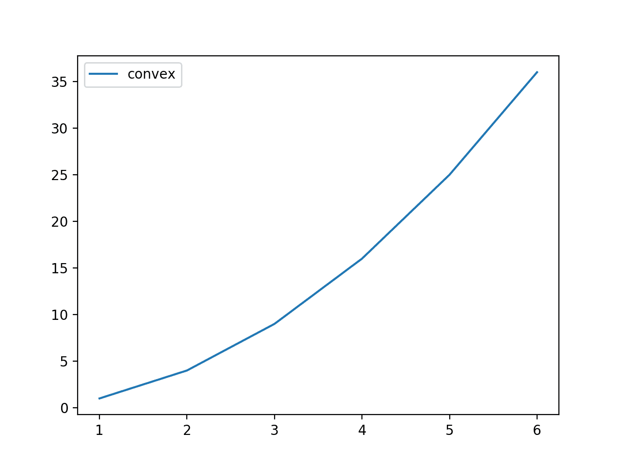
Line Plot of Dice Roll Outcomes vs. Convex Payoff Function
Jensen’s Inequality suggests that the mean of the payoffs will always be larger than or equal to the payoff of the mean outcome.
Recall that the range of possible outcomes is [1,2,3,4,5,6] and the mean of the possible outcome is 3.5, therefore we know that the payoff of the mean outcome is 3.5^2 or 12.25. Our intuition wants us to believe that the mean of the payoffs would also be about 12.25, but this intuition is wrong.
To confirm that our intuition is wrong, let’s compare these two values over all possible outcomes.
The complete example is listed below.
|
1 2 3 4 5 6 7 8 9 10 11 12 13 14 15 16 17 |
# example comparing mean convex transform vs convex transform for mean value from numpy import mean # transform function def payoff(x): return x**2 # each possible roll of the dice outcomes = [1, 2, 3, 4, 5, 6] # payoff for each roll payoffs = [payoff(value) for value in outcomes] # mean of the payoffs of the outcomes v1 = mean(payoffs) print(v1) # payoff of the mean outcome v2 = payoff(mean(outcomes)) print(v2) |
Running the example, we can see that our intuition for the payoff for the mean outcome is correct; the value is 12.25, as we expected.
We can see that the intuition breaks down and that the mean payoff value is slightly higher than 12.25.
Recall that the mean (arithmetic mean) is really just a sum of the values, normalized by the number of values. Now consider that we are summing over much larger values in the case if the payoffs, specifically [1, 4, 9, 16, 25, 36], which sums to 91. This pulls our mean higher.
The intuition is that because the function is convex, the transformed values are always going to be larger than the raw outcome values, on average, or any other sum type operation we want to use.
|
1 2 |
15.166666666666666 12.25 |
There is one more step that might help with the intuition, and that is the idea of sampling.
We have looked at an example of calculating the payoff for all possible outcomes, but this is unusual. Instead, we are more likely to sample a number of outcomes from a domain and calculate the payoff for each.
We can implement this by rolling the dice many times, e.g. 50, and calculate the payoff for each outcome, then compare the mean payoff to the payoff of the mean outcome.
|
1 2 3 |
... # roll the dice [1,6] many times (e.g. 50) outcomes = randint(1, 7, 50) |
Intuitively, we would expect the mean outcome to be close to the idealized value of 3.5 and therefore the payoff for the mean value to be close to 3^2 or 12.25. We would also expect the mean of the payoff values to be close to 15.1.
The randomness allows many repeated outcomes and an important distribution of each outcome, therefore the mean of the payoffs and the payoff of the means will vary each repetition of this experiment. We will repeat the experiment 10 times. Each repetition, we expect the inequality to hold.
The complete example is listed below.
|
1 2 3 4 5 6 7 8 9 10 11 12 13 14 15 16 17 18 19 20 21 22 23 24 |
# example of repeated trials of Jensen's Inequality from numpy.random import randint from numpy import mean # transform function def payoff(x): return x**2 # repeated trials n_trials = 10 n_samples = 50 for i in range(n_trials): # roll the dice [1,6] many times (e.g. 50) outcomes = randint(1, 7, n_samples) # calculate the payoff for each outcome payoffs = [payoff(x) for x in outcomes] # calculate the mean of the payoffs v1 = mean(payoffs) # calculate the payoff of the mean outcome v2 = payoff(mean(outcomes)) # confirm the expectation assert v1 >= v2 # summarize the result print('>%d: %.2f >= %.2f' % (i, v1, v2)) |
Running the example, we can see that the two mean values move around a fair bit across the trials.
Note: your specific results will vary given the stochastic nature of the experiment.
For example, we see mean payoff values as low as 12.20 and as high as 16.88. We see the payoff from the mean outcome as low as 9.36 and as high as 14.29.
Nevertheless, for any single experiment, Jensen’s Inequality holds.
|
1 2 3 4 5 6 7 8 9 10 |
>0: 12.20 >= 9.73 >1: 14.14 >= 10.37 >2: 16.88 >= 13.84 >3: 15.68 >= 12.39 >4: 13.92 >= 11.56 >5: 15.44 >= 12.39 >6: 15.62 >= 13.10 >7: 17.50 >= 14.29 >8: 12.38 >= 9.36 >9: 15.52 >= 12.39 |
Now that we have some intuition for Jensen’s Inequality, let’s look at some cases where it is used.
Arithmetic and Geometric Means Example
A common application of Jensen’s Inequality is in the comparison of arithmetic mean (AM) and geometric mean (GM).
Recall the arithmetic mean is the sum of the observations divided by the number of observations and is only appropriate when all of the observations have the same scale.
For example:
- (10 + 20) / 2 = 15
When the sample observations have different scales, e.g. refer to different things, then the geometric mean is used.
This involves first calculating the product of the observations and then taking the nth root for the result, where n is the number of values. For two values, we would use the square root, for three values, we would use the cube root, and so on.
For example:
- sqrt(10 * 20) = 14.14
The nth root can also be calculated using the 1/n exponent, making the notation and calculation simpler. Therefore, our geometric mean can be calculated as:
- (10 * 20)^(1/2) = 14.14
The sample values would be our outcomes and the nth root would be our payoff function, and the nth root is a concave function.
For more on the difference between the arithmetic and geometric mean, see:
At first glance, it might not be obvious how these two functions are related, but in fact, the arithmetic mean also uses the nth root payoff function with n=1, which has no effect.
Recall that the nth root and logarithms are inverse functions of each other. We can establish their relationship more clearly if we first use the inverse of the nth root or log as the payoff function f().
In the case of the geometric mean, or GM, we are calculating the mean of the log outcome:
- GM = mean( log(outcome) )
In the case of the arithmetic means or AM, we are calculating the log of the mean outcome.
- AM = log( mean(outcome) )
The log function is concave, therefore given our knowledge of Jensen’s Inequality, we know that:
- geometric mean(x) <= arithmetic mean(x)
The convention when describing the inequality of the AM and GM is to list the AM first, therefore, the inequality can be summarized as:
- arithmetic mean(x) >= geometric mean(x)
or
- AM >= GM
We can make this clear with a small worked example with our game of dice rolls in [1-6] and a log payoff function.
The complete example is listed below.
|
1 2 3 4 5 6 7 8 9 10 11 12 13 14 15 16 17 18 19 20 21 22 |
# example comparing the log geometric mean and the log arithmetic mean from numpy import mean from numpy import log from matplotlib import pyplot # transform function def payoff(x): return log(x) # each possible roll of the dice outcomes = [1, 2, 3, 4, 5, 6] # payoff for each roll payoffs = [payoff(value) for value in outcomes] # mean of the payoffs of the outcomes (log gm) gm = mean(payoffs) # payoff of the mean outcome (log am) am = payoff(mean(outcomes)) # print results print('Log AM %.2f >= Log GM %.2f' % (am, gm)) # line plot of outcome vs payoff pyplot.plot(outcomes, payoffs) pyplot.show() |
Running the example confirms our expectation that the log arithmetic mean is greater than the log geometric mean.
|
1 |
Log AM 1.25 >= Log GM 1.10 |
A line plot of all possible outcomes versus the payoffs is also created showing the concave nature of the log() function.
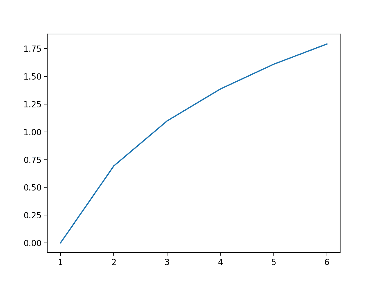
Line Plot of All Dice Outcomes and Log Payoffs Showing Concave Function
We can now remove the log from both the mean calculations. This can be easily done by using an inverse log function to each side, or the nth root.
Removing the log and replacing it with an nth root for the geometric means gives us the normal geometric mean calculation:
- geometric mean = [1 * 2 * 3 * 4 * 5 * 6]^(1/6)
Recall that the 6th root can also be calculated via the exponent of 1/6.
The arithmetic mean can be calculated with the 1st root, which does nothing, e.g. the mean with the exponent 1/1 or raised to the first power, therefore the arithmetic mean is:
- arithmetic = [1 + 2 + 3 + 4 + 5 + 6]/6
The square root function is also concave like the log function, and the Jensen’s Inequality still holds:
- arithmetic mean(x) >= geometric mean(x)
This is referred to as the inequality of arithmetic and geometric means, or AM-GM inequality for short.
This inequality is important when working with financial time series, such as calculating the rate of return.
For example, the average rate of return can be calculated over an interval such as monthly over one year. It could be calculated using the arithmetic mean, but this value would be optimistic (a larger value) and would exclude the reinvestment of returns and would assume any losses would be topped up at the start of each period.
Instead, the geometric mean must be used to give the real average rate of return over the interval (a smaller value), correctly taking into account losses with reinvesting and compounding gains.
The arithmetic average return is always larger than the geometric average return, and in this case, is misleading.
Other Applications
Jensen’s Inequality is a useful tool in mathematics, specifically in applied fields such as probability and statistics.
For example, it is often used as a tool in mathematical proofs.
It is also used to make claims about a function where little is known or needs to be known about the distribution. One example is the use of the inequality in defining the lower bound on the probability of a random variable.
Jensen’s Inequality also provides the mathematical basis for the idea of “antifragility” in Nassim Taleb’s 2012 book titled “Antifragile.” The example of a convex payoff function for dice rolls described above was inspired by a section of this book (Chapter 19).
Further Reading
This section provides more resources on the topic if you are looking to go deeper.
Books
- Real & Complex Analysis, 1987.
- Inequalities, 1988.
- Antifragile: Things That Gain from Disorder, 2012.
Articles
- Linear map, Wikipedia.
- Jensen’s inequality, Wikipedia.
- Inequality of arithmetic and geometric means, Wikipedia.
- Geometric mean, Wikipedia.
- nth root, Wikipedia.
Summary
In this tutorial, you discovered Jensen’s Inequality in mathematics and statistics.
Specifically, you learned:
- The intuition of linear mappings does not hold for nonlinear functions.
- The mean of a convex function of a variable is always greater than the function of the mean variable, called Jensen’s Inequality.
- A common application of the inequality is in the comparison of arithmetic and geometric means when averaging the financial returns for a time interval.
Do you have any questions?
Ask your questions in the comments below and I will do my best to answer.
Get a Handle on Probability for Machine Learning!
Develop Your Understanding of Probability
...with just a few lines of python codeDiscover how in my new Ebook:
Probability for Machine Learning
It provides self-study tutorials and end-to-end projects on:
Bayes Theorem, Bayesian Optimization, Distributions, Maximum Likelihood, Cross-Entropy, Calibrating Models
and much more...


This means rolling a 3 will give a payoff of 3 * 0.3 or 1.5. (?)
In what context Andy?
I assume this is a spelling error and it should be 3 * 0.5 or 1.5
Thanks, fixed.
Great Job, thx.
One minor correction:
“f(x) == x^2 is an exponential convex function. This is because as x increases, the output of the transform function f() increases at an exponential rate.”
We say that f() increase quadratically and not exponentially since x (our input) is not in the exponent.
Quite right, thanks!
Quadratic the value is the variable, exponential the exponent is the variable.