It is often desirable to quantify the difference between probability distributions for a given random variable.
This occurs frequently in machine learning, when we may be interested in calculating the difference between an actual and observed probability distribution.
This can be achieved using techniques from information theory, such as the Kullback-Leibler Divergence (KL divergence), or relative entropy, and the Jensen-Shannon Divergence that provides a normalized and symmetrical version of the KL divergence. These scoring methods can be used as shortcuts in the calculation of other widely used methods, such as mutual information for feature selection prior to modeling, and cross-entropy used as a loss function for many different classifier models.
In this post, you will discover how to calculate the divergence between probability distributions.
After reading this post, you will know:
Statistical distance is the general idea of calculating the difference between statistical objects like different probability distributions for a random variable.
Kullback-Leibler divergence calculates a score that measures the divergence of one probability distribution from another.
Jensen-Shannon divergence extends KL divergence to calculate a symmetrical score and distance measure of one probability distribution from another.
Kick-start your project with my new book Probability for Machine Learning, including step-by-step tutorials and the Python source code files for all examples.
Let’s get started.
Update Oct/2019: Added a description of the alternative form of the equation (thanks Ori).
How to Calculate the Distance Between Probability Distributions Photo by Paxson Woelber, some rights reserved.
Overview
This tutorial is divided into three parts; they are:
Statistical Distance
Kullback-Leibler Divergence
Jensen-Shannon Divergence
Statistical Distance
There are many situations where we may want to compare two probability distributions.
Specifically, we may have a single random variable and two different probability distributions for the variable, such as a true distribution and an approximation of that distribution.
In situations like this, it can be useful to quantify the difference between the distributions. Generally, this is referred to as the problem of calculating the statistical distance between two statistical objects, e.g. probability distributions.
One approach is to calculate a distance measure between the two distributions. This can be challenging as it can be difficult to interpret the measure.
Instead, it is more common to calculate a divergence between two probability distributions. A divergence is like a measure but is not symmetrical. This means that a divergence is a scoring of how one distribution differs from another, where calculating the divergence for distributions P and Q would give a different score from Q and P.
Divergence scores are an important foundation for many different calculations in information theory and more generally in machine learning. For example, they provide shortcuts for calculating scores such as mutual information (information gain) and cross-entropy used as a loss function for classification models.
Divergence scores are also used directly as tools for understanding complex modeling problems, such as approximating a target probability distribution when optimizing generative adversarial network (GAN) models.
Two commonly used divergence scores from information theory are Kullback-Leibler Divergence and Jensen-Shannon Divergence.
We will take a closer look at both of these scores in the following section.
Want to Learn Probability for Machine Learning
Take my free 7-day email crash course now (with sample code).
Click to sign-up and also get a free PDF Ebook version of the course.
Kullback-Leibler Divergence
The Kullback-Leibler Divergence score, or KL divergence score, quantifies how much one probability distribution differs from another probability distribution.
The KL divergence between two distributions Q and P is often stated using the following notation:
KL(P || Q)
Where the “||” operator indicates “divergence” or Ps divergence from Q.
KL divergence can be calculated as the negative sum of probability of each event in P multiplied by the log of the probability of the event in Q over the probability of the event in P.
KL(P || Q) = – sum x in X P(x) * log(Q(x) / P(x))
The value within the sum is the divergence for a given event.
This is the same as the positive sum of probability of each event in P multiplied by the log of the probability of the event in P over the probability of the event in Q (e.g. the terms in the fraction are flipped). This is the more common implementation used in practice.
KL(P || Q) = sum x in X P(x) * log(P(x) / Q(x))
The intuition for the KL divergence score is that when the probability for an event from P is large, but the probability for the same event in Q is small, there is a large divergence. When the probability from P is small and the probability from Q is large, there is also a large divergence, but not as large as the first case.
It can be used to measure the divergence between discrete and continuous probability distributions, where in the latter case the integral of the events is calculated instead of the sum of the probabilities of the discrete events.
One way to measure the dissimilarity of two probability distributions, p and q, is known as the Kullback-Leibler divergence (KL divergence) or relative entropy.
The log can be base-2 to give units in “bits,” or the natural logarithm base-e with units in “nats.” When the score is 0, it suggests that both distributions are identical, otherwise the score is positive.
Importantly, the KL divergence score is not symmetrical, for example:
KL(P || Q) != KL(Q || P)
It is named for the two authors of the method Solomon Kullback and Richard Leibler, and is sometimes referred to as “relative entropy.”
This is known as the relative entropy or Kullback-Leibler divergence, or KL divergence, between the distributions p(x) and q(x).
If we are attempting to approximate an unknown probability distribution, then the target probability distribution from data is P and Q is our approximation of the distribution.
In this case, the KL divergence summarizes the number of additional bits (i.e. calculated with the base-2 logarithm) required to represent an event from the random variable. The better our approximation, the less additional information is required.
… the KL divergence is the average number of extra bits needed to encode the data, due to the fact that we used distribution q to encode the data instead of the true distribution p.
Running the example first calculates the divergence of P from Q as just under 2 bits, then Q from P as just over 2 bits.
This is intuitive if we consider P has large probabilities when Q is small, giving P less divergence than Q from P as Q has more small probabilities when P has large probabilities. There is more divergence in this second case.
1
2
KL(P || Q): 1.927 bits
KL(Q || P): 2.022 bits
If we change log2() to the natural logarithm log() function, the result is in nats, as follows:
1
2
# KL(P || Q): 1.336 nats
# KL(Q || P): 1.401 nats
The SciPy library provides the kl_div() function for calculating the KL divergence, although with a different definition as defined here. It also provides the rel_entr() function for calculating the relative entropy, which matches the definition of KL divergence here. This is odd as “relative entropy” is often used as a synonym for “KL divergence.”
Nevertheless, we can calculate the KL divergence using the rel_entr() SciPy function and confirm that our manual calculation is correct.
The rel_entr() function takes lists of probabilities across all events from each probability distribution as arguments and returns a list of divergences for each event. These can be summed to give the KL divergence. The calculation uses the natural logarithm instead of log base-2 so the units are in nats instead of bits.
The complete example using SciPy to calculate KL(P || Q) and KL(Q || P) for the same probability distributions used above is listed below:
1
2
3
4
5
6
7
8
9
10
11
# example of calculating the kl divergence (relative entropy) with scipy
from scipy.special import rel_entr
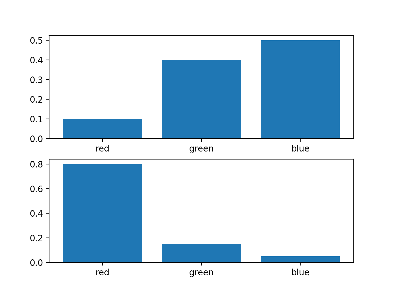
# define distributions
p=[0.10,0.40,0.50]
q=[0.80,0.15,0.05]
# calculate (P || Q)
kl_pq=rel_entr(p,q)
print('KL(P || Q): %.3f nats'%sum(kl_pq))
# calculate (Q || P)
kl_qp=rel_entr(q,p)
print('KL(Q || P): %.3f nats'%sum(kl_qp))
Running the example, we can see that the calculated divergences match our manual calculation of about 1.3 nats and about 1.4 nats for KL(P || Q) and KL(Q || P) respectively.
1
2
KL(P || Q): 1.336 nats
KL(Q || P): 1.401 nats
Jensen-Shannon Divergence
The Jensen-Shannon divergence, or JS divergence for short, is another way to quantify the difference (or similarity) between two probability distributions.
It uses the KL divergence to calculate a normalized score that is symmetrical. This means that the divergence of P from Q is the same as Q from P, or stated formally:
JS(P || Q) == JS(Q || P)
The JS divergence can be calculated as follows:
JS(P || Q) = 1/2 * KL(P || M) + 1/2 * KL(Q || M)
Where M is calculated as:
M = 1/2 * (P + Q)
And KL() is calculated as the KL divergence described in the previous section.
It is more useful as a measure as it provides a smoothed and normalized version of KL divergence, with scores between 0 (identical) and 1 (maximally different), when using the base-2 logarithm.
The square root of the score gives a quantity referred to as the Jensen-Shannon distance, or JS distance for short.
We can make the JS divergence concrete with a worked example.
First, we can define a function to calculate the JS divergence that uses the kl_divergence() function prepared in the previous section.
We can then test this function using the same probability distributions used in the previous section.
First, we will calculate the JS divergence score for the distributions, then calculate the square root of the score to give the JS distance between the distributions. For example:
1
2
3
4
5
...
# calculate JS(P || Q)
js_pq=js_divergence(p,q)
print('JS(P || Q) divergence: %.3f bits'%js_pq)
print('JS(P || Q) distance: %.3f'%sqrt(js_pq))
This can then be repeated for the reverse case to show that the divergence is symmetrical, unlike the KL divergence.
1
2
3
4
5
...
# calculate JS(Q || P)
js_qp=js_divergence(q,p)
print('JS(Q || P) divergence: %.3f bits'%js_qp)
print('JS(Q || P) distance: %.3f'%sqrt(js_qp))
Tying this together, the complete example of calculating the JS divergence and JS distance is listed below.
1
2
3
4
5
6
7
8
9
10
11
12
13
14
15
16
17
18
19
20
21
22
23
24
25
# example of calculating the js divergence between two mass functions
Running the example shows that the JS divergence between the distributions is about 0.4 bits and that the distance is about 0.6.
We can see that the calculation is symmetrical, giving the same score and distance measure for JS(P || Q) and JS(Q || P).
1
2
3
4
JS(P || Q) divergence: 0.420 bits
JS(P || Q) distance: 0.648
JS(Q || P) divergence: 0.420 bits
JS(Q || P) distance: 0.648
The SciPy library provides an implementation of the JS distance via the jensenshannon() function.
It takes arrays of probabilities across all events from each probability distribution as arguments and returns the JS distance score, not a divergence score. We can use this function to confirm our manual calculation of the JS distance.
The complete example is listed below.
1
2
3
4
5
6
7
8
9
10
11
12
# calculate the jensen-shannon distance metric
from scipy.spatial.distance import jensenshannon
from numpy import asarray
# define distributions
p=asarray([0.10,0.40,0.50])
q=asarray([0.80,0.15,0.05])
# calculate JS(P || Q)
js_pq=jensenshannon(p,q,base=2)
print('JS(P || Q) Distance: %.3f'%js_pq)
# calculate JS(Q || P)
js_qp=jensenshannon(q,p,base=2)
print('JS(Q || P) Distance: %.3f'%js_qp)
Running the example, we can confirm the distance score matches our manual calculation of 0.648, and that the distance calculation is symmetrical as expected.
1
2
JS(P || Q) Distance: 0.648
JS(Q || P) Distance: 0.648
Further Reading
This section provides more resources on the topic if you are looking to go deeper.
In this post, you discovered how to calculate the divergence between probability distributions.
Specifically, you learned:
Statistical distance is the general idea of calculating the difference between statistical objects like different probability distributions for a random variable.
Kullback-Leibler divergence calculates a score that measures the divergence of one probability distribution from another.
Jensen-Shannon divergence extends KL divergence to calculate a symmetrical score and distance measure of one probability distribution from another.
Do you have any questions?
Ask your questions in the comments below and I will do my best to answer.
It provides self-study tutorials and end-to-end projects on: Bayes Theorem, Bayesian Optimization, Distributions, Maximum Likelihood, Cross-Entropy, Calibrating Models
and much more...
Hi Jason,
This might be answered in your blog but I am struggling to figure it out. Suppose you are given from start histograms of two samples. Given this much, how should I proceed to calculate the KL divergence of the two data sets?
Do you have written an article on the “correlation coefficient calculation for categorical as well as numerical/continuous data”?
Sometimes it seems to be misleading for me and I got confused about what is the right way to calculate the correlation coefficient when data contains categorical as well as continuous features?
If yes then kindly provide me the pointer to the blog.
Hi Jason, do you know if there is a threshold value for each of these two metrics that corresponds to an acceptable approximation of one distribution by another? I feel that all probability metrics are pretty subjectives in the end. Thanks!
When the distribution contains certain probabilities (0 and 1), then the KL divergence will match the cross entropy, as the entropy for the distribution will be zero.
Does that help?
I don’t think they are subjective, they are measuring real data.
Hi Jason, thank you for the article! I would like to ask if the following makes sense:
I have performed unsupervised clustering on several images using the Gaussian Mixture Modelling method and I want to find out the similarity between 2 images, where each image is from a different cluster.
Does it make sense to measure the similarity between the 2 images by calculating the Jensen-Shannon Distance using the 2 images and treating each image as a different distribution (https://docs.scipy.org/doc/scipy/reference/generated/scipy.spatial.distance.jensenshannon.html)?
So I am working on a problem similar to stuffs what I am asking. I have a data sample, and it’s histogram is plotted following some random uncommon distribution. Since I need probabilities for calculating KL divergence, I tried the Kernel non parametric estimation(about which I read in your blog on probability density) to estimate a density function. Then using the density function I obtained the KL divergence.
So my concern is if I am doing something wrong or not.
Hi,
Is it possible to find KL divergence for dependent variable’s probability distribution in multivariate dataset?If yes how? Please give example . Here dependent variable depends on multiple independent variables.
Thank you
Hello,
I mean if dataset is multivariate how do we compute KL divergence ? suppose every instance is in the form of (x,y) where x={x1,x,2,…xn} i.e.number of x attributes(independent) and y depends on these x values . How to compute KL divergence for such type of multivariate dataset
Hi,
Your post was great! But the kl_divergence(p, q) function you wrote, this is only for discrete variable, right? What to do for continuous variable?
Okay, another thing, I know the values in p or q need to be between 0-1. But should the sum of all the values of p be 1?
And also, using the rel_entr() function, I got negative value for some example I was trying, is it possible? If it is, what does it mean?
Thank you so much for your reply. After searching many resources, at one place I found that the value of KL divergence can’t be negative. There was some facts about my data which may not be acceptable by KL divergence that’s why was generating the negative value. Thank you.
Hi Jason,
Do you have any idea on estimating KL (P(x)’ll Q(x)) when we just have Monte Carlo samples from P, and Q is a know normal distribution, say N (0,1)?
Thanks!
The thing is that for P distribution, I just have the samples, so I do not know how to compute the probability. unless I discretize the distribution to use the normalized frequency of the samples in each bin as the probability values, but it causes additional estimation error due to the discretization.
In my project i have 10 discrete probability distributions. I have calculated the KL divergence for each pair of distributions and have created a KL divergence score matrix [10X10]. With this matrix, i am then applying hierarchical clustering to cluster distributions that are similar.
My question is: Is there any way the KL divergence score be used to understand how much similar the pair of distributions are? Understand 0 means identical and the KL value can go upto infinity. For example, What does a KL value of 0.5 represent? Can this be equated to some sort of 90% or 80% similarity between the distributions?
The question is basically to identify a threshold KL similarity score between two probability distributions to understand whether they can be clustered. The threshold may depend on the business problem we are trying to solve, but how do we justify any threshold KL divergence score?
This is a great post Jason! thank you!
One question – if JS can be used to calculate the “distance” between two distributions, can you explain when do I use this distance metric vs using something like cosine distance?
I have been using the cosine distance for quite some time now, and i would like to understand if there are specific situations when it is more appropriate to use JS over cosine.
Curiously Coding FoxahOctober 10, 2020 at 4:30 am#
I’ve got four (non-linear, tree-based) models in production and using the average of them as the served prediction. We get ground truth data immediately.
During training the optimized candidate models had very similar performance, so I decided to deploy all of them and take the average and served that as the prediction. With the intention of figuring which one would really be best at a later point.
That later point has come.
Out of these four models two seem fit the ground truth distribution quite well, at least by examining the KDE plot of the predicted values against the ground truth distribution
I was initially thinking of doing a pairwise 2-sample KS Test (each model against ground truth) to see if the predicted values from the models come from the same distribution as the ground truth.
But I talked myself out of it. Mostly because I have 50,000+ predictions and I figured that a sample size that large will result in a small p-value anyway.
I then turned my attention to KL divergence. Something I have never used before.
Would comparing the KL-Divergence between each model’s prediction and the ground truth be a good way to assess model fit?
If so, how would I go about doing this? scipy.stats.kl_div outputs an array which contains (I assume) the divergence between the prediction and ground truth.
Would I just take the sum of the array and call that the Divergence between the model and ground truth?
Hopefully I don’t sound crazy or too much like I don’t know what I’m doing or talking about. Because I kinda don’t, but not too much.
Curiously Coding FoxahOctober 14, 2020 at 7:02 am#
Hi Jason! Thanks for the response. I have another version of this question
Would it make sense to use KL-Divergence to measure the difference in predictions versus ground truth for a regression problem?
I’ve tuned four models and serve the average as a prediction in the production environment.
I plotted the ecdf and kde for each model’s prediction versus the ground truth, and I want a way to capture the closeness of the distributions in one number that I can track over time.
I use an evaluation metric for MAE for assessing performance, but I also wanted a way to capture how similar or different the shapes of the distributions for prediction and ground truth are in a single number.
One question – Could you please explain in more details how LK-Divergence is not the same for both cases (p to q – q to p)? In other word, I can’t understand the intuitive (quoted below); the subtraction of probabilities for each event is the same regardless the direction (p to q – q to p)
”This is intuitive if we consider P has large probabilities when Q is small, giving P less divergence than Q from P as Q has more small probabilities when P has large probabilities.”
Hi Jason, the article is well written. I just have a remark about the KL divergence. when you calculate it in the example you got
KL(P || Q): 1.927 bits
based on the definition the result should be negative, did you use the absolute value to infer the number of bits?
Good question, please note the we are using the alternate positive calculation that is more common in practice, discussed in the section titled “Kullback-Leibler Divergence”.
Hi Jason,
Thanks for the post!
You write the the KL is not symmetrical, “for example …”. Mathematically speaking, non-symmetric means precisely that KL(P,Q) = KL(Q, P) is not always true, so imho it’s better to replace “for example” with “that is, the equality … doesn’t always hold” or “that is, usually KL(P,Q) != KL(Q,P).
* KL(P || Q) = sum x in X P(x) * log(P(x) / Q(x))
The intuition for the KL divergence score is that when the probability for an event from P is large, but the probability for the same event in Q is small, there is a large divergence. When the probability from P is small and the probability from Q is large, there is also a large divergence, but not as large as the first case.
It seems to be, that if P(p) is small and P(q) for the same event is large, then the fraction in the log is < 1. That would give a negative result, and as such, shouldn't it actually cancel out some of the divergence? Given we are not taking an absolute value of the terms of the sum.
Therefore, yes, if P is large but Q is small, there is large divergence, but in the inverse situation there is actually "negative" divergence.
Is there something I am missing here?
Thank you for this post, very useful, just wanted to clear up some confusion regarding this point.
* KL(P || Q) = sum x in X P(x) * log(P(x) / Q(x))
The intuition for the KL divergence score is that when the probability for an event from P is large, but the probability for the same event in Q is small, there is a large divergence. When the probability from P is small and the probability from Q is large, there is also a large divergence, but not as large as the first case.
Wouldn’t the divergence in the second case be negative, meaning it would be cancelling out somewhat with the other cases where P > Q? Why do we not take absolute value of all the terms in the sum instead?
I am not sure why I get NAN for kl. y_train is 0.7 of y and y_val is 0.3 of y.
p = y_train
q = y_val
kl_pq = rel_entr(p, q)
print(‘KL(P || Q): %.3f nats’ % sum(kl_pq))
kl_qp = rel_entr(q, p)
print(‘KL(Q || P): %.3f nats’ % sum(kl_qp))
In case we have the same type of data (PDFs values), and we need to do classification using the Random forest and the KL-divergence. Is there any way to check which one outperforms the other?
Or just I need to try both methods and check which one outperforms the other?
Hi, I would like to find out how do I intepret the Jensen-Shannon distance, for e.g. does a value of JSD = 0.5 means that two distributions overlap by 50%? What is the threshold of JS distance to tell if the data drift is significant or not? Thank you.


 from Scratch in Python")

Hi Jason, you mentioned it’s the negative sum in the formula, but the in the code is a positive sum.
Right!
We can also use an alternative form: KL(P || Q) = sum x in X P(x) * log(P(x) / Q(x))
This is the version that we implement in practice.
I have updated the post, thanks!
Hi Jason,
This might be answered in your blog but I am struggling to figure it out. Suppose you are given from start histograms of two samples. Given this much, how should I proceed to calculate the KL divergence of the two data sets?
You need the data, histograms (plots) are insufficient.
Hello Jason,
Do you have written an article on the “correlation coefficient calculation for categorical as well as numerical/continuous data”?
Sometimes it seems to be misleading for me and I got confused about what is the right way to calculate the correlation coefficient when data contains categorical as well as continuous features?
If yes then kindly provide me the pointer to the blog.
Thanking you,
Saurabh
Yes, I will schedule a post on the topic of cross-type correlation.
Thanks for the suggestion.
Hi Jason,
Can you please provide a code for KL and JS divergence if the given distributions are continuous probability distributions?
Thanks for the suggestion.
Hi Jason,
it would be more pythonic to use the zip method instead of range(len()) :
[pi * np.log2(qi/pi) for pi, qi in zip(p,q)]
see here for instance :
https://docs.quantifiedcode.com/python-anti-patterns/readability/not_using_zip_to_iterate_over_a_pair_of_lists.html
Yes, thanks!
Hi Jason, do you know if there is a threshold value for each of these two metrics that corresponds to an acceptable approximation of one distribution by another? I feel that all probability metrics are pretty subjectives in the end. Thanks!
When the distribution contains certain probabilities (0 and 1), then the KL divergence will match the cross entropy, as the entropy for the distribution will be zero.
Does that help?
I don’t think they are subjective, they are measuring real data.
Hi Jason, thank you for the article! I would like to ask if the following makes sense:
I have performed unsupervised clustering on several images using the Gaussian Mixture Modelling method and I want to find out the similarity between 2 images, where each image is from a different cluster.
Does it make sense to measure the similarity between the 2 images by calculating the Jensen-Shannon Distance using the 2 images and treating each image as a different distribution (https://docs.scipy.org/doc/scipy/reference/generated/scipy.spatial.distance.jensenshannon.html)?
Thank you.
Perhaps try it and see if it is appropriate for your data.
I believe image similarity is a large field of study, I recommend performing a review of the literature to see what methods work well generally.
So I am working on a problem similar to stuffs what I am asking. I have a data sample, and it’s histogram is plotted following some random uncommon distribution. Since I need probabilities for calculating KL divergence, I tried the Kernel non parametric estimation(about which I read in your blog on probability density) to estimate a density function. Then using the density function I obtained the KL divergence.
So my concern is if I am doing something wrong or not.
Your approach sounds reasonable.
Hi,
Is it possible to find KL divergence for dependent variable’s probability distribution in multivariate dataset?If yes how? Please give example . Here dependent variable depends on multiple independent variables.
Thank you
Sorry, I don’t understand, can you please elaborate what you mean?
Hello,
I mean if dataset is multivariate how do we compute KL divergence ? suppose every instance is in the form of (x,y) where x={x1,x,2,…xn} i.e.number of x attributes(independent) and y depends on these x values . How to compute KL divergence for such type of multivariate dataset
The approach is general as far as I understand, you can calculate divergence between univariate and multivariate probability distributions.
Perhaps this will help:
https://en.wikipedia.org/wiki/Kullback%E2%80%93Leibler_divergence#Multivariate_normal_distributions
ok thanks
Hi,
Your post was great! But the kl_divergence(p, q) function you wrote, this is only for discrete variable, right? What to do for continuous variable?
Thanks.
I described it for a discrete variable, but you can use it for continuous as well.
Okay, another thing, I know the values in p or q need to be between 0-1. But should the sum of all the values of p be 1?
And also, using the rel_entr() function, I got negative value for some example I was trying, is it possible? If it is, what does it mean?
The sum of the probabilities for all evens must sum to one.
P and Q are distributions of events. All events for P must sum to 1. All events for Q must sum to 1.
I don’t undertand a negative kl divergenve, sorry.
Thank you so much for your reply. After searching many resources, at one place I found that the value of KL divergence can’t be negative. There was some facts about my data which may not be acceptable by KL divergence that’s why was generating the negative value. Thank you.
I’m happy to hear that.
Hi Jason,
Do you have any idea on estimating KL (P(x)’ll Q(x)) when we just have Monte Carlo samples from P, and Q is a know normal distribution, say N (0,1)?
Thanks!
As long as you have a probability for the same events in each distribution, I think you’re good to go.
Perhaps you need to interpolate some samples.
The thing is that for P distribution, I just have the samples, so I do not know how to compute the probability. unless I discretize the distribution to use the normalized frequency of the samples in each bin as the probability values, but it causes additional estimation error due to the discretization.
One approach might be to use an empirical distribution function:
https://machinelearningmastery.com/empirical-distribution-function-in-python/
Hi Jason
Do you have any tutorial on how to approximate the KL-Divergence between two GMMs?
Sorry I do not.
HI Jason, Great article!
In my project i have 10 discrete probability distributions. I have calculated the KL divergence for each pair of distributions and have created a KL divergence score matrix [10X10]. With this matrix, i am then applying hierarchical clustering to cluster distributions that are similar.
My question is: Is there any way the KL divergence score be used to understand how much similar the pair of distributions are? Understand 0 means identical and the KL value can go upto infinity. For example, What does a KL value of 0.5 represent? Can this be equated to some sort of 90% or 80% similarity between the distributions?
The question is basically to identify a threshold KL similarity score between two probability distributions to understand whether they can be clustered. The threshold may depend on the business problem we are trying to solve, but how do we justify any threshold KL divergence score?
If you use log base 2, you can interpret the result in bits.
E.g. how much more information or surprise there is in one distribution of events compared to another.
Thank you very much Jason!
You’re welcome.
How do we interpret the results in bits, as in how do we find an ideal threshold for this method?
Hi Nandana…The following resource may be of interest:
https://towardsdatascience.com/light-on-math-machine-learning-intuitive-guide-to-understanding-kl-divergence-2b382ca2b2a8
This is a great post Jason! thank you!
One question – if JS can be used to calculate the “distance” between two distributions, can you explain when do I use this distance metric vs using something like cosine distance?
I have been using the cosine distance for quite some time now, and i would like to understand if there are specific situations when it is more appropriate to use JS over cosine.
Thanks again!
NIkhil
Cosine distance is between two vectors. The above method are for the distance between two distributions.
I’ve got four (non-linear, tree-based) models in production and using the average of them as the served prediction. We get ground truth data immediately.
During training the optimized candidate models had very similar performance, so I decided to deploy all of them and take the average and served that as the prediction. With the intention of figuring which one would really be best at a later point.
That later point has come.
Out of these four models two seem fit the ground truth distribution quite well, at least by examining the KDE plot of the predicted values against the ground truth distribution
I was initially thinking of doing a pairwise 2-sample KS Test (each model against ground truth) to see if the predicted values from the models come from the same distribution as the ground truth.
But I talked myself out of it. Mostly because I have 50,000+ predictions and I figured that a sample size that large will result in a small p-value anyway.
I then turned my attention to KL divergence. Something I have never used before.
Would comparing the KL-Divergence between each model’s prediction and the ground truth be a good way to assess model fit?
If so, how would I go about doing this? scipy.stats.kl_div outputs an array which contains (I assume) the divergence between the prediction and ground truth.
Would I just take the sum of the array and call that the Divergence between the model and ground truth?
Hopefully I don’t sound crazy or too much like I don’t know what I’m doing or talking about. Because I kinda don’t, but not too much.
Thank you
Yes, perhaps try it and see.
You would average the divergence for each prediction.
This will give you ideas:
https://machinelearningmastery.com/cross-entropy-for-machine-learning/
Hi Jason! Thanks for the response. I have another version of this question
Would it make sense to use KL-Divergence to measure the difference in predictions versus ground truth for a regression problem?
I’ve tuned four models and serve the average as a prediction in the production environment.
I plotted the ecdf and kde for each model’s prediction versus the ground truth, and I want a way to capture the closeness of the distributions in one number that I can track over time.
I use an evaluation metric for MAE for assessing performance, but I also wanted a way to capture how similar or different the shapes of the distributions for prediction and ground truth are in a single number.
Hmm, great question.
Cautiously, I would say yes, but double check the literature to see if there is a more appropriate divergence measure.
Hi Jason, thank you for this great article!
One question – Could you please explain in more details how LK-Divergence is not the same for both cases (p to q – q to p)? In other word, I can’t understand the intuitive (quoted below); the subtraction of probabilities for each event is the same regardless the direction (p to q – q to p)
”This is intuitive if we consider P has large probabilities when Q is small, giving P less divergence than Q from P as Q has more small probabilities when P has large probabilities.”
Think of it as “relative entropy”, e.g. the first distribution relative to the second. If the order is changed, the relative entropy must change.
Thanks Jason! it’s much clearer now.
You’re welcome.
Hi Jason,
What if the p and q are multidimensions like shape (32,50)? Then how do we calculate the kl?
Not sure what you mean, sorry.
p and q are probability distributions for events.
Hi Jason, the article is well written. I just have a remark about the KL divergence. when you calculate it in the example you got
KL(P || Q): 1.927 bits
based on the definition the result should be negative, did you use the absolute value to infer the number of bits?
Good question, please note the we are using the alternate positive calculation that is more common in practice, discussed in the section titled “Kullback-Leibler Divergence”.
Hi Jason,
Thanks for the post!
You write the the KL is not symmetrical, “for example …”. Mathematically speaking, non-symmetric means precisely that KL(P,Q) = KL(Q, P) is not always true, so imho it’s better to replace “for example” with “that is, the equality … doesn’t always hold” or “that is, usually KL(P,Q) != KL(Q,P).
Thanks for the suggestion.
Hello Jason,
If I want to use the KL for evaluating my GAN and calculate it between a real distribution and generated distribution, How can I do that?
I used your script and make P as a real distribution and Q as a generated distribution but it returns nan values.
So, Can you help me?
I’m not sure it would be an appropriate metric for a GAN.
Instead, I recommend the metrics listed here:
https://machinelearningmastery.com/how-to-evaluate-generative-adversarial-networks/
Yes, I read it thank you.
I read papers for GAN and they used KL as matric for example MAD-GAN:
https://openaccess.thecvf.com/content_cvpr_2018/papers/Ghosh_Multi-Agent_Diverse_Generative_CVPR_2018_paper.pdf
Interesting. Thanks for sharing.
Hey there. Could you possibly speak to how this might be expanded to a Markov process?
Thanks for the suggestion.
Hi Jason,
Thanks for the great post. Is there a preferred way to compute KL if p(k)=0 (division by zero) or q(k) (log of 0)?
Typically we add tiny values to parameters to avoid zeros when coding the thing up for real.
Hello, I am wondering about this statement:
* KL(P || Q) = sum x in X P(x) * log(P(x) / Q(x))
The intuition for the KL divergence score is that when the probability for an event from P is large, but the probability for the same event in Q is small, there is a large divergence. When the probability from P is small and the probability from Q is large, there is also a large divergence, but not as large as the first case.
It seems to be, that if P(p) is small and P(q) for the same event is large, then the fraction in the log is < 1. That would give a negative result, and as such, shouldn't it actually cancel out some of the divergence? Given we are not taking an absolute value of the terms of the sum.
Therefore, yes, if P is large but Q is small, there is large divergence, but in the inverse situation there is actually "negative" divergence.
Is there something I am missing here?
Thank you for this post, very useful, just wanted to clear up some confusion regarding this point.
Perhaps you can test your intuition with some worked examples/real numbers.
Hello, I was wondering about this statement:
* KL(P || Q) = sum x in X P(x) * log(P(x) / Q(x))
The intuition for the KL divergence score is that when the probability for an event from P is large, but the probability for the same event in Q is small, there is a large divergence. When the probability from P is small and the probability from Q is large, there is also a large divergence, but not as large as the first case.
Wouldn’t the divergence in the second case be negative, meaning it would be cancelling out somewhat with the other cases where P > Q? Why do we not take absolute value of all the terms in the sum instead?
Run real numbers through and see.
I am not sure why I get NAN for kl. y_train is 0.7 of y and y_val is 0.3 of y.
p = y_train
q = y_val
kl_pq = rel_entr(p, q)
print(‘KL(P || Q): %.3f nats’ % sum(kl_pq))
kl_qp = rel_entr(q, p)
print(‘KL(Q || P): %.3f nats’ % sum(kl_qp))
result:
KL(P || Q): nan nats
KL(Q || P): nan nats
I don’t have any nan in y itself.
Both p and q must be all non-negative or otherwise your rel_entr will give you nan. Then sum will be nan too.
Hi Jason,
I am not sure why I get one of my KLs as a negative value. I have provided for you the p and q arrays (I converted them to numpy arrays)
p: [6.33527306 0.17195741 0.01810078 0.01810078]
q: [7.36958404 0.09665028 0.02416257 0.02416257]
KL(p, q): -1.2543610466991473
KL(q, p): 1.547671142537377
JS(P || Q) Distance: 0.042
JS(Q || P) Distance: 0.042
KL formula involves log, and log can return negative value
How can someone find convergence in Generative adversarial networks ?
Hi Dipnakar…The following resource may help to address many of your queries regarding GANs:
https://machinelearningmastery.com/resources-for-getting-started-with-generative-adversarial-networks/
Hi,
In case we have the same type of data (PDFs values), and we need to do classification using the Random forest and the KL-divergence. Is there any way to check which one outperforms the other?
Or just I need to try both methods and check which one outperforms the other?
Hi Wesam…The following may be helpful in terms of comparing the performance of machine learning models:
https://machinelearningmastery.com/statistical-significance-tests-for-comparing-machine-learning-algorithms/
Hi, I would like to find out how do I intepret the Jensen-Shannon distance, for e.g. does a value of JSD = 0.5 means that two distributions overlap by 50%? What is the threshold of JS distance to tell if the data drift is significant or not? Thank you.