In this tutorial you are going to learn about the Naive Bayes algorithm including how it works and how to implement it from scratch in Python (without libraries).
We can use probability to make predictions in machine learning. Perhaps the most widely used example is called the Naive Bayes algorithm. Not only is it straightforward to understand, but it also achieves surprisingly good results on a wide range of problems.
After completing this tutorial you will know:
- How to calculate the probabilities required by the Naive Bayes algorithm.
- How to implement the Naive Bayes algorithm from scratch.
- How to apply Naive Bayes to a real-world predictive modeling problem.
Kick-start your project with my new book Machine Learning Algorithms From Scratch, including step-by-step tutorials and the Python source code files for all examples.
Let’s get started.
- Update Dec/2014: Original implementation.
- Update Oct/2019: Rewrote the tutorial and code from the ground-up.
Code a Naive Bayes Classifier From Scratch in Python (with no libraries)
Photo by Matt Buck, some rights reserved
Overview
This section provides a brief overview of the Naive Bayes algorithm and the Iris flowers dataset that we will use in this tutorial.
Naive Bayes
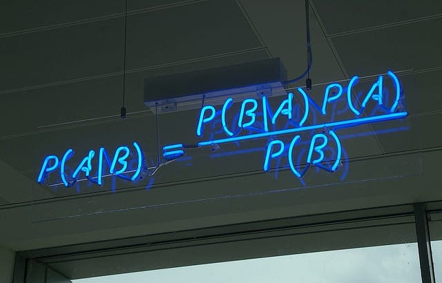
Bayes’ Theorem provides a way that we can calculate the probability of a piece of data belonging to a given class, given our prior knowledge. Bayes’ Theorem is stated as:
- P(class|data) = (P(data|class) * P(class)) / P(data)
Where P(class|data) is the probability of class given the provided data.
For an in-depth introduction to Bayes Theorem, see the tutorial:
Naive Bayes is a classification algorithm for binary (two-class) and multiclass classification problems. It is called Naive Bayes or idiot Bayes because the calculations of the probabilities for each class are simplified to make their calculations tractable.
Rather than attempting to calculate the probabilities of each attribute value, they are assumed to be conditionally independent given the class value.
This is a very strong assumption that is most unlikely in real data, i.e. that the attributes do not interact. Nevertheless, the approach performs surprisingly well on data where this assumption does not hold.
For an in-depth introduction to Naive Bayes, see the tutorial:
Iris Flower Species Dataset
In this tutorial we will use the Iris Flower Species Dataset.
The Iris Flower Dataset involves predicting the flower species given measurements of iris flowers.
It is a multiclass classification problem. The number of observations for each class is balanced. There are 150 observations with 4 input variables and 1 output variable. The variable names are as follows:
- Sepal length in cm.
- Sepal width in cm.
- Petal length in cm.
- Petal width in cm.
- Class
A sample of the first 5 rows is listed below.
|
1 2 3 4 5 6 |
5.1,3.5,1.4,0.2,Iris-setosa 4.9,3.0,1.4,0.2,Iris-setosa 4.7,3.2,1.3,0.2,Iris-setosa 4.6,3.1,1.5,0.2,Iris-setosa 5.0,3.6,1.4,0.2,Iris-setosa ... |
The baseline performance on the problem is approximately 33%.
Download the dataset and save it into your current working directory with the filename iris.csv.
Naive Bayes Tutorial (in 5 easy steps)
First we will develop each piece of the algorithm in this section, then we will tie all of the elements together into a working implementation applied to a real dataset in the next section.
This Naive Bayes tutorial is broken down into 5 parts:
- Step 1: Separate By Class.
- Step 2: Summarize Dataset.
- Step 3: Summarize Data By Class.
- Step 4: Gaussian Probability Density Function.
- Step 5: Class Probabilities.
These steps will provide the foundation that you need to implement Naive Bayes from scratch and apply it to your own predictive modeling problems.
Note: This tutorial assumes that you are using Python 3. If you need help installing Python, see this tutorial:
Note: if you are using Python 2.7, you must change all calls to the items() function on dictionary objects to iteritems().
Step 1: Separate By Class
We will need to calculate the probability of data by the class they belong to, the so-called base rate.
This means that we will first need to separate our training data by class. A relatively straightforward operation.
We can create a dictionary object where each key is the class value and then add a list of all the records as the value in the dictionary.
Below is a function named separate_by_class() that implements this approach. It assumes that the last column in each row is the class value.
|
1 2 3 4 5 6 7 8 9 10 |
# Split the dataset by class values, returns a dictionary def separate_by_class(dataset): separated = dict() for i in range(len(dataset)): vector = dataset[i] class_value = vector[-1] if (class_value not in separated): separated[class_value] = list() separated[class_value].append(vector) return separated |
We can contrive a small dataset to test out this function.
|
1 2 3 4 5 6 7 8 9 10 11 |
X1 X2 Y 3.393533211 2.331273381 0 3.110073483 1.781539638 0 1.343808831 3.368360954 0 3.582294042 4.67917911 0 2.280362439 2.866990263 0 7.423436942 4.696522875 1 5.745051997 3.533989803 1 9.172168622 2.511101045 1 7.792783481 3.424088941 1 7.939820817 0.791637231 1 |
We can plot this dataset and use separate colors for each class.
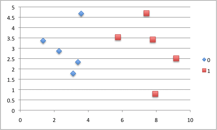
Scatter Plot of Small Contrived Dataset for Testing the Naive Bayes Algorithm
Putting this all together, we can test our separate_by_class() function on the contrived dataset.
|
1 2 3 4 5 6 7 8 9 10 11 12 13 14 15 16 17 18 19 20 21 22 23 24 25 26 27 28 29 |
# Example of separating data by class value # Split the dataset by class values, returns a dictionary def separate_by_class(dataset): separated = dict() for i in range(len(dataset)): vector = dataset[i] class_value = vector[-1] if (class_value not in separated): separated[class_value] = list() separated[class_value].append(vector) return separated # Test separating data by class dataset = [[3.393533211,2.331273381,0], [3.110073483,1.781539638,0], [1.343808831,3.368360954,0], [3.582294042,4.67917911,0], [2.280362439,2.866990263,0], [7.423436942,4.696522875,1], [5.745051997,3.533989803,1], [9.172168622,2.511101045,1], [7.792783481,3.424088941,1], [7.939820817,0.791637231,1]] separated = separate_by_class(dataset) for label in separated: print(label) for row in separated[label]: print(row) |
Running the example sorts observations in the dataset by their class value, then prints the class value followed by all identified records.
|
1 2 3 4 5 6 7 8 9 10 11 12 |
0 [3.393533211, 2.331273381, 0] [3.110073483, 1.781539638, 0] [1.343808831, 3.368360954, 0] [3.582294042, 4.67917911, 0] [2.280362439, 2.866990263, 0] 1 [7.423436942, 4.696522875, 1] [5.745051997, 3.533989803, 1] [9.172168622, 2.511101045, 1] [7.792783481, 3.424088941, 1] [7.939820817, 0.791637231, 1] |
Next we can start to develop the functions needed to collect statistics.
Step 2: Summarize Dataset
We need two statistics from a given set of data.
We’ll see how these statistics are used in the calculation of probabilities in a few steps. The two statistics we require from a given dataset are the mean and the standard deviation (average deviation from the mean).
The mean is the average value and can be calculated as:
- mean = sum(x)/n * count(x)
Where x is the list of values or a column we are looking.
Below is a small function named mean() that calculates the mean of a list of numbers.
|
1 2 3 |
# Calculate the mean of a list of numbers def mean(numbers): return sum(numbers)/float(len(numbers)) |
The sample standard deviation is calculated as the mean difference from the mean value. This can be calculated as:
- standard deviation = sqrt((sum i to N (x_i – mean(x))^2) / N-1)
You can see that we square the difference between the mean and a given value, calculate the average squared difference from the mean, then take the square root to return the units back to their original value.
Below is a small function named standard_deviation() that calculates the standard deviation of a list of numbers. You will notice that it calculates the mean. It might be more efficient to calculate the mean of a list of numbers once and pass it to the standard_deviation() function as a parameter. You can explore this optimization if you’re interested later.
|
1 2 3 4 5 6 7 |
from math import sqrt # Calculate the standard deviation of a list of numbers def stdev(numbers): avg = mean(numbers) variance = sum([(x-avg)**2 for x in numbers]) / float(len(numbers)-1) return sqrt(variance) |
We require the mean and standard deviation statistics to be calculated for each input attribute or each column of our data.
We can do that by gathering all of the values for each column into a list and calculating the mean and standard deviation on that list. Once calculated, we can gather the statistics together into a list or tuple of statistics. Then, repeat this operation for each column in the dataset and return a list of tuples of statistics.
Below is a function named summarize_dataset() that implements this approach. It uses some Python tricks to cut down on the number of lines required.
|
1 2 3 4 5 |
# Calculate the mean, stdev and count for each column in a dataset def summarize_dataset(dataset): summaries = [(mean(column), stdev(column), len(column)) for column in zip(*dataset)] del(summaries[-1]) return summaries |
The first trick is the use of the zip() function that will aggregate elements from each provided argument. We pass in the dataset to the zip() function with the * operator that separates the dataset (that is a list of lists) into separate lists for each row. The zip() function then iterates over each element of each row and returns a column from the dataset as a list of numbers. A clever little trick.
We then calculate the mean, standard deviation and count of rows in each column. A tuple is created from these 3 numbers and a list of these tuples is stored. We then remove the statistics for the class variable as we will not need these statistics.
Let’s test all of these functions on our contrived dataset from above. Below is the complete example.
|
1 2 3 4 5 6 7 8 9 10 11 12 13 14 15 16 17 18 19 20 21 22 23 24 25 26 27 28 29 30 31 32 |
# Example of summarizing a dataset from math import sqrt # Calculate the mean of a list of numbers def mean(numbers): return sum(numbers)/float(len(numbers)) # Calculate the standard deviation of a list of numbers def stdev(numbers): avg = mean(numbers) variance = sum([(x-avg)**2 for x in numbers]) / float(len(numbers)-1) return sqrt(variance) # Calculate the mean, stdev and count for each column in a dataset def summarize_dataset(dataset): summaries = [(mean(column), stdev(column), len(column)) for column in zip(*dataset)] del(summaries[-1]) return summaries # Test summarizing a dataset dataset = [[3.393533211,2.331273381,0], [3.110073483,1.781539638,0], [1.343808831,3.368360954,0], [3.582294042,4.67917911,0], [2.280362439,2.866990263,0], [7.423436942,4.696522875,1], [5.745051997,3.533989803,1], [9.172168622,2.511101045,1], [7.792783481,3.424088941,1], [7.939820817,0.791637231,1]] summary = summarize_dataset(dataset) print(summary) |
Running the example prints out the list of tuples of statistics on each of the two input variables.
Interpreting the results, we can see that the mean value of X1 is 5.178333386499999 and the standard deviation of X1 is 2.7665845055177263.
|
1 |
[(5.178333386499999, 2.7665845055177263, 10), (2.9984683241, 1.218556343617447, 10)] |
Now we are ready to use these functions on each group of rows in our dataset.
Step 3: Summarize Data By Class
We require statistics from our training dataset organized by class.
Above, we have developed the separate_by_class() function to separate a dataset into rows by class. And we have developed summarize_dataset() function to calculate summary statistics for each column.
We can put all of this together and summarize the columns in the dataset organized by class values.
Below is a function named summarize_by_class() that implements this operation. The dataset is first split by class, then statistics are calculated on each subset. The results in the form of a list of tuples of statistics are then stored in a dictionary by their class value.
|
1 2 3 4 5 6 7 |
# Split dataset by class then calculate statistics for each row def summarize_by_class(dataset): separated = separate_by_class(dataset) summaries = dict() for class_value, rows in separated.items(): summaries[class_value] = summarize_dataset(rows) return summaries |
Again, let’s test out all of these behaviors on our contrived dataset.
|
1 2 3 4 5 6 7 8 9 10 11 12 13 14 15 16 17 18 19 20 21 22 23 24 25 26 27 28 29 30 31 32 33 34 35 36 37 38 39 40 41 42 43 44 45 46 47 48 49 50 51 52 53 54 |
# Example of summarizing data by class value from math import sqrt # Split the dataset by class values, returns a dictionary def separate_by_class(dataset): separated = dict() for i in range(len(dataset)): vector = dataset[i] class_value = vector[-1] if (class_value not in separated): separated[class_value] = list() separated[class_value].append(vector) return separated # Calculate the mean of a list of numbers def mean(numbers): return sum(numbers)/float(len(numbers)) # Calculate the standard deviation of a list of numbers def stdev(numbers): avg = mean(numbers) variance = sum([(x-avg)**2 for x in numbers]) / float(len(numbers)-1) return sqrt(variance) # Calculate the mean, stdev and count for each column in a dataset def summarize_dataset(dataset): summaries = [(mean(column), stdev(column), len(column)) for column in zip(*dataset)] del(summaries[-1]) return summaries # Split dataset by class then calculate statistics for each row def summarize_by_class(dataset): separated = separate_by_class(dataset) summaries = dict() for class_value, rows in separated.items(): summaries[class_value] = summarize_dataset(rows) return summaries # Test summarizing by class dataset = [[3.393533211,2.331273381,0], [3.110073483,1.781539638,0], [1.343808831,3.368360954,0], [3.582294042,4.67917911,0], [2.280362439,2.866990263,0], [7.423436942,4.696522875,1], [5.745051997,3.533989803,1], [9.172168622,2.511101045,1], [7.792783481,3.424088941,1], [7.939820817,0.791637231,1]] summary = summarize_by_class(dataset) for label in summary: print(label) for row in summary[label]: print(row) |
Running this example calculates the statistics for each input variable and prints them organized by class value. Interpreting the results, we can see that the X1 values for rows for class 0 have a mean value of 2.7420144012.
|
1 2 3 4 5 6 |
0 (2.7420144012, 0.9265683289298018, 5) (3.0054686692, 1.1073295894898725, 5) 1 (7.6146523718, 1.2344321550313704, 5) (2.9914679790000003, 1.4541931384601618, 5) |
There is one more piece we need before we start calculating probabilities.
Step 4: Gaussian Probability Density Function
Calculating the probability or likelihood of observing a given real-value like X1 is difficult.
One way we can do this is to assume that X1 values are drawn from a distribution, such as a bell curve or Gaussian distribution.
A Gaussian distribution can be summarized using only two numbers: the mean and the standard deviation. Therefore, with a little math, we can estimate the probability of a given value. This piece of math is called a Gaussian Probability Distribution Function (or Gaussian PDF) and can be calculated as:
- f(x) = (1 / sqrt(2 * PI) * sigma) * exp(-((x-mean)^2 / (2 * sigma^2)))
Where sigma is the standard deviation for x, mean is the mean for x and PI is the value of pi.
Below is a function that implements this. I tried to split it up to make it more readable.
|
1 2 3 4 |
# Calculate the Gaussian probability distribution function for x def calculate_probability(x, mean, stdev): exponent = exp(-((x-mean)**2 / (2 * stdev**2 ))) return (1 / (sqrt(2 * pi) * stdev)) * exponent |
Let’s test it out to see how it works. Below are some worked examples.
|
1 2 3 4 5 6 7 8 9 10 11 12 13 14 |
# Example of Gaussian PDF from math import sqrt from math import pi from math import exp # Calculate the Gaussian probability distribution function for x def calculate_probability(x, mean, stdev): exponent = exp(-((x-mean)**2 / (2 * stdev**2 ))) return (1 / (sqrt(2 * pi) * stdev)) * exponent # Test Gaussian PDF print(calculate_probability(1.0, 1.0, 1.0)) print(calculate_probability(2.0, 1.0, 1.0)) print(calculate_probability(0.0, 1.0, 1.0)) |
Running it prints the probability of some input values. You can see that when the value is 1 and the mean and standard deviation is 1 our input is the most likely (top of the bell curve) and has the probability of 0.39.
We can see that when we keep the statistics the same and change the x value to 1 standard deviation either side of the mean value (2 and 0 or the same distance either side of the bell curve) the probabilities of those input values are the same at 0.24.
|
1 2 3 |
0.3989422804014327 0.24197072451914337 0.24197072451914337 |
Now that we have all the pieces in place, let’s see how we can calculate the probabilities we need for the Naive Bayes classifier.
Step 5: Class Probabilities
Now it is time to use the statistics calculated from our training data to calculate probabilities for new data.
Probabilities are calculated separately for each class. This means that we first calculate the probability that a new piece of data belongs to the first class, then calculate probabilities that it belongs to the second class, and so on for all the classes.
The probability that a piece of data belongs to a class is calculated as follows:
- P(class|data) = P(X|class) * P(class)
You may note that this is different from the Bayes Theorem described above.
The division has been removed to simplify the calculation.
This means that the result is no longer strictly a probability of the data belonging to a class. The value is still maximized, meaning that the calculation for the class that results in the largest value is taken as the prediction. This is a common implementation simplification as we are often more interested in the class prediction rather than the probability.
The input variables are treated separately, giving the technique it’s name “naive“. For the above example where we have 2 input variables, the calculation of the probability that a row belongs to the first class 0 can be calculated as:
- P(class=0|X1,X2) = P(X1|class=0) * P(X2|class=0) * P(class=0)
Now you can see why we need to separate the data by class value. The Gaussian Probability Density function in the previous step is how we calculate the probability of a real value like X1 and the statistics we prepared are used in this calculation.
Below is a function named calculate_class_probabilities() that ties all of this together.
It takes a set of prepared summaries and a new row as input arguments.
First the total number of training records is calculated from the counts stored in the summary statistics. This is used in the calculation of the probability of a given class or P(class) as the ratio of rows with a given class of all rows in the training data.
Next, probabilities are calculated for each input value in the row using the Gaussian probability density function and the statistics for that column and of that class. Probabilities are multiplied together as they accumulated.
This process is repeated for each class in the dataset.
Finally a dictionary of probabilities is returned with one entry for each class.
|
1 2 3 4 5 6 7 8 9 10 |
# Calculate the probabilities of predicting each class for a given row def calculate_class_probabilities(summaries, row): total_rows = sum([summaries[label][0][2] for label in summaries]) probabilities = dict() for class_value, class_summaries in summaries.items(): probabilities[class_value] = summaries[class_value][0][2]/float(total_rows) for i in range(len(class_summaries)): mean, stdev, count = class_summaries[i] probabilities[class_value] *= calculate_probability(row[i], mean, stdev) return probabilities |
Let’s tie this together with an example on the contrived dataset.
The example below first calculates the summary statistics by class for the training dataset, then uses these statistics to calculate the probability of the first record belonging to each class.
|
1 2 3 4 5 6 7 8 9 10 11 12 13 14 15 16 17 18 19 20 21 22 23 24 25 26 27 28 29 30 31 32 33 34 35 36 37 38 39 40 41 42 43 44 45 46 47 48 49 50 51 52 53 54 55 56 57 58 59 60 61 62 63 64 65 66 67 68 69 70 |
# Example of calculating class probabilities from math import sqrt from math import pi from math import exp # Split the dataset by class values, returns a dictionary def separate_by_class(dataset): separated = dict() for i in range(len(dataset)): vector = dataset[i] class_value = vector[-1] if (class_value not in separated): separated[class_value] = list() separated[class_value].append(vector) return separated # Calculate the mean of a list of numbers def mean(numbers): return sum(numbers)/float(len(numbers)) # Calculate the standard deviation of a list of numbers def stdev(numbers): avg = mean(numbers) variance = sum([(x-avg)**2 for x in numbers]) / float(len(numbers)-1) return sqrt(variance) # Calculate the mean, stdev and count for each column in a dataset def summarize_dataset(dataset): summaries = [(mean(column), stdev(column), len(column)) for column in zip(*dataset)] del(summaries[-1]) return summaries # Split dataset by class then calculate statistics for each row def summarize_by_class(dataset): separated = separate_by_class(dataset) summaries = dict() for class_value, rows in separated.items(): summaries[class_value] = summarize_dataset(rows) return summaries # Calculate the Gaussian probability distribution function for x def calculate_probability(x, mean, stdev): exponent = exp(-((x-mean)**2 / (2 * stdev**2 ))) return (1 / (sqrt(2 * pi) * stdev)) * exponent # Calculate the probabilities of predicting each class for a given row def calculate_class_probabilities(summaries, row): total_rows = sum([summaries[label][0][2] for label in summaries]) probabilities = dict() for class_value, class_summaries in summaries.items(): probabilities[class_value] = summaries[class_value][0][2]/float(total_rows) for i in range(len(class_summaries)): mean, stdev, _ = class_summaries[i] probabilities[class_value] *= calculate_probability(row[i], mean, stdev) return probabilities # Test calculating class probabilities dataset = [[3.393533211,2.331273381,0], [3.110073483,1.781539638,0], [1.343808831,3.368360954,0], [3.582294042,4.67917911,0], [2.280362439,2.866990263,0], [7.423436942,4.696522875,1], [5.745051997,3.533989803,1], [9.172168622,2.511101045,1], [7.792783481,3.424088941,1], [7.939820817,0.791637231,1]] summaries = summarize_by_class(dataset) probabilities = calculate_class_probabilities(summaries, dataset[0]) print(probabilities) |
Running the example prints the probabilities calculated for each class.
We can see that the probability of the first row belonging to the 0 class (0.0503) is higher than the probability of it belonging to the 1 class (0.0001). We would therefore correctly conclude that it belongs to the 0 class.
|
1 |
{0: 0.05032427673372075, 1: 0.00011557718379945765} |
Now that we have seen how to implement the Naive Bayes algorithm, let’s apply it to the Iris flowers dataset.
Iris Flower Species Case Study
This section applies the Naive Bayes algorithm to the Iris flowers dataset.
The first step is to load the dataset and convert the loaded data to numbers that we can use with the mean and standard deviation calculations. For this we will use the helper function load_csv() to load the file, str_column_to_float() to convert string numbers to floats and str_column_to_int() to convert the class column to integer values.
We will evaluate the algorithm using k-fold cross-validation with 5 folds. This means that 150/5=30 records will be in each fold. We will use the helper functions evaluate_algorithm() to evaluate the algorithm with cross-validation and accuracy_metric() to calculate the accuracy of predictions.
A new function named predict() was developed to manage the calculation of the probabilities of a new row belonging to each class and selecting the class with the largest probability value.
Another new function named naive_bayes() was developed to manage the application of the Naive Bayes algorithm, first learning the statistics from a training dataset and using them to make predictions for a test dataset.
If you would like more help with the data loading functions used below, see the tutorial:
If you would like more help with the way the model is evaluated using cross validation, see the tutorial:
The complete example is listed below.
|
1 2 3 4 5 6 7 8 9 10 11 12 13 14 15 16 17 18 19 20 21 22 23 24 25 26 27 28 29 30 31 32 33 34 35 36 37 38 39 40 41 42 43 44 45 46 47 48 49 50 51 52 53 54 55 56 57 58 59 60 61 62 63 64 65 66 67 68 69 70 71 72 73 74 75 76 77 78 79 80 81 82 83 84 85 86 87 88 89 90 91 92 93 94 95 96 97 98 99 100 101 102 103 104 105 106 107 108 109 110 111 112 113 114 115 116 117 118 119 120 121 122 123 124 125 126 127 128 129 130 131 132 133 134 135 136 137 138 139 140 141 142 143 144 145 146 147 148 149 150 151 152 153 154 155 156 157 158 |
# Naive Bayes On The Iris Dataset from csv import reader from random import seed from random import randrange from math import sqrt from math import exp from math import pi # Load a CSV file def load_csv(filename): dataset = list() with open(filename, 'r') as file: csv_reader = reader(file) for row in csv_reader: if not row: continue dataset.append(row) return dataset # Convert string column to float def str_column_to_float(dataset, column): for row in dataset: row[column] = float(row[column].strip()) # Convert string column to integer def str_column_to_int(dataset, column): class_values = [row[column] for row in dataset] unique = set(class_values) lookup = dict() for i, value in enumerate(unique): lookup[value] = i for row in dataset: row[column] = lookup[row[column]] return lookup # Split a dataset into k folds def cross_validation_split(dataset, n_folds): dataset_split = list() dataset_copy = list(dataset) fold_size = int(len(dataset) / n_folds) for _ in range(n_folds): fold = list() while len(fold) < fold_size: index = randrange(len(dataset_copy)) fold.append(dataset_copy.pop(index)) dataset_split.append(fold) return dataset_split # Calculate accuracy percentage def accuracy_metric(actual, predicted): correct = 0 for i in range(len(actual)): if actual[i] == predicted[i]: correct += 1 return correct / float(len(actual)) * 100.0 # Evaluate an algorithm using a cross validation split def evaluate_algorithm(dataset, algorithm, n_folds, *args): folds = cross_validation_split(dataset, n_folds) scores = list() for fold in folds: train_set = list(folds) train_set.remove(fold) train_set = sum(train_set, []) test_set = list() for row in fold: row_copy = list(row) test_set.append(row_copy) row_copy[-1] = None predicted = algorithm(train_set, test_set, *args) actual = [row[-1] for row in fold] accuracy = accuracy_metric(actual, predicted) scores.append(accuracy) return scores # Split the dataset by class values, returns a dictionary def separate_by_class(dataset): separated = dict() for i in range(len(dataset)): vector = dataset[i] class_value = vector[-1] if (class_value not in separated): separated[class_value] = list() separated[class_value].append(vector) return separated # Calculate the mean of a list of numbers def mean(numbers): return sum(numbers)/float(len(numbers)) # Calculate the standard deviation of a list of numbers def stdev(numbers): avg = mean(numbers) variance = sum([(x-avg)**2 for x in numbers]) / float(len(numbers)-1) return sqrt(variance) # Calculate the mean, stdev and count for each column in a dataset def summarize_dataset(dataset): summaries = [(mean(column), stdev(column), len(column)) for column in zip(*dataset)] del(summaries[-1]) return summaries # Split dataset by class then calculate statistics for each row def summarize_by_class(dataset): separated = separate_by_class(dataset) summaries = dict() for class_value, rows in separated.items(): summaries[class_value] = summarize_dataset(rows) return summaries # Calculate the Gaussian probability distribution function for x def calculate_probability(x, mean, stdev): exponent = exp(-((x-mean)**2 / (2 * stdev**2 ))) return (1 / (sqrt(2 * pi) * stdev)) * exponent # Calculate the probabilities of predicting each class for a given row def calculate_class_probabilities(summaries, row): total_rows = sum([summaries[label][0][2] for label in summaries]) probabilities = dict() for class_value, class_summaries in summaries.items(): probabilities[class_value] = summaries[class_value][0][2]/float(total_rows) for i in range(len(class_summaries)): mean, stdev, _ = class_summaries[i] probabilities[class_value] *= calculate_probability(row[i], mean, stdev) return probabilities # Predict the class for a given row def predict(summaries, row): probabilities = calculate_class_probabilities(summaries, row) best_label, best_prob = None, -1 for class_value, probability in probabilities.items(): if best_label is None or probability > best_prob: best_prob = probability best_label = class_value return best_label # Naive Bayes Algorithm def naive_bayes(train, test): summarize = summarize_by_class(train) predictions = list() for row in test: output = predict(summarize, row) predictions.append(output) return(predictions) # Test Naive Bayes on Iris Dataset seed(1) filename = 'iris.csv' dataset = load_csv(filename) for i in range(len(dataset[0])-1): str_column_to_float(dataset, i) # convert class column to integers str_column_to_int(dataset, len(dataset[0])-1) # evaluate algorithm n_folds = 5 scores = evaluate_algorithm(dataset, naive_bayes, n_folds) print('Scores: %s' % scores) print('Mean Accuracy: %.3f%%' % (sum(scores)/float(len(scores)))) |
Running the example prints the mean classification accuracy scores on each cross-validation fold as well as the mean accuracy score.
We can see that the mean accuracy of about 95% is dramatically better than the baseline accuracy of 33%.
|
1 2 |
Scores: [93.33333333333333, 96.66666666666667, 100.0, 93.33333333333333, 93.33333333333333] Mean Accuracy: 95.333% |
We can fit the model on the entire dataset and then use the model to make predictions for new observations (rows of data).
For example, the model is just a set of probabilities calculated via the summarize_by_class() function.
|
1 2 3 |
... # fit model model = summarize_by_class(dataset) |
Once calculated, we can use them in a call to the predict() function with a row representing our new observation to predict the class label.
|
1 2 3 |
... # predict the label label = predict(model, row) |
We also might like to know the class label (string) for a prediction. We can update the str_column_to_int() function to print the mapping of string class names to integers so we can interpret the prediction by the model.
|
1 2 3 4 5 6 7 8 9 10 11 |
# Convert string column to integer def str_column_to_int(dataset, column): class_values = [row[column] for row in dataset] unique = set(class_values) lookup = dict() for i, value in enumerate(unique): lookup[value] = i print('[%s] => %d' % (value, i)) for row in dataset: row[column] = lookup[row[column]] return lookup |
Tying this together, a complete example of fitting the Naive Bayes model on the entire dataset and making a single prediction for a new observation is listed below.
|
1 2 3 4 5 6 7 8 9 10 11 12 13 14 15 16 17 18 19 20 21 22 23 24 25 26 27 28 29 30 31 32 33 34 35 36 37 38 39 40 41 42 43 44 45 46 47 48 49 50 51 52 53 54 55 56 57 58 59 60 61 62 63 64 65 66 67 68 69 70 71 72 73 74 75 76 77 78 79 80 81 82 83 84 85 86 87 88 89 90 91 92 93 94 95 96 97 98 99 100 101 102 103 104 105 106 107 108 109 |
# Make Predictions with Naive Bayes On The Iris Dataset from csv import reader from math import sqrt from math import exp from math import pi # Load a CSV file def load_csv(filename): dataset = list() with open(filename, 'r') as file: csv_reader = reader(file) for row in csv_reader: if not row: continue dataset.append(row) return dataset # Convert string column to float def str_column_to_float(dataset, column): for row in dataset: row[column] = float(row[column].strip()) # Convert string column to integer def str_column_to_int(dataset, column): class_values = [row[column] for row in dataset] unique = set(class_values) lookup = dict() for i, value in enumerate(unique): lookup[value] = i print('[%s] => %d' % (value, i)) for row in dataset: row[column] = lookup[row[column]] return lookup # Split the dataset by class values, returns a dictionary def separate_by_class(dataset): separated = dict() for i in range(len(dataset)): vector = dataset[i] class_value = vector[-1] if (class_value not in separated): separated[class_value] = list() separated[class_value].append(vector) return separated # Calculate the mean of a list of numbers def mean(numbers): return sum(numbers)/float(len(numbers)) # Calculate the standard deviation of a list of numbers def stdev(numbers): avg = mean(numbers) variance = sum([(x-avg)**2 for x in numbers]) / float(len(numbers)-1) return sqrt(variance) # Calculate the mean, stdev and count for each column in a dataset def summarize_dataset(dataset): summaries = [(mean(column), stdev(column), len(column)) for column in zip(*dataset)] del(summaries[-1]) return summaries # Split dataset by class then calculate statistics for each row def summarize_by_class(dataset): separated = separate_by_class(dataset) summaries = dict() for class_value, rows in separated.items(): summaries[class_value] = summarize_dataset(rows) return summaries # Calculate the Gaussian probability distribution function for x def calculate_probability(x, mean, stdev): exponent = exp(-((x-mean)**2 / (2 * stdev**2 ))) return (1 / (sqrt(2 * pi) * stdev)) * exponent # Calculate the probabilities of predicting each class for a given row def calculate_class_probabilities(summaries, row): total_rows = sum([summaries[label][0][2] for label in summaries]) probabilities = dict() for class_value, class_summaries in summaries.items(): probabilities[class_value] = summaries[class_value][0][2]/float(total_rows) for i in range(len(class_summaries)): mean, stdev, _ = class_summaries[i] probabilities[class_value] *= calculate_probability(row[i], mean, stdev) return probabilities # Predict the class for a given row def predict(summaries, row): probabilities = calculate_class_probabilities(summaries, row) best_label, best_prob = None, -1 for class_value, probability in probabilities.items(): if best_label is None or probability > best_prob: best_prob = probability best_label = class_value return best_label # Make a prediction with Naive Bayes on Iris Dataset filename = 'iris.csv' dataset = load_csv(filename) for i in range(len(dataset[0])-1): str_column_to_float(dataset, i) # convert class column to integers str_column_to_int(dataset, len(dataset[0])-1) # fit model model = summarize_by_class(dataset) # define a new record row = [5.7,2.9,4.2,1.3] # predict the label label = predict(model, row) print('Data=%s, Predicted: %s' % (row, label)) |
Running the data first summarizes the mapping of class labels to integers and then fits the model on the entire dataset.
Then a new observation is defined (in this case I took a row from the dataset), and a predicted label is calculated. In this case our observation is predicted as belonging to class 1 which we know is “Iris-versicolor“.
|
1 2 3 4 5 |
[Iris-virginica] => 0 [Iris-versicolor] => 1 [Iris-setosa] => 2 Data=[5.7, 2.9, 4.2, 1.3], Predicted: 1 |
Extensions
This section lists extensions to the tutorial that you may wish to explore.
- Log Probabilities: The conditional probabilities for each class given an attribute value are small. When they are multiplied together they result in very small values, which can lead to floating point underflow (numbers too small to represent in Python). A common fix for this is to add the log of the probabilities together. Research and implement this improvement.
- Nominal Attributes: Update the implementation to support nominal attributes. This is much similar and the summary information you can collect for each attribute is the ratio of category values for each class. Dive into the references for more information.
- Different Density Function (bernoulli or multinomial): We have looked at Gaussian Naive Bayes, but you can also look at other distributions. Implement a different distribution such as multinomial, bernoulli or kernel naive bayes that make different assumptions about the distribution of attribute values and/or their relationship with the class value.
If you try any of these extensions, let me know in the comments below.
Further Reading
Tutorials
- A Gentle Introduction to Bayes Theorem for Machine Learning
- How to Develop a Naive Bayes Classifier from Scratch in Python
- Naive Bayes Tutorial for Machine Learning
- Naive Bayes for Machine Learning
- Better Naive Bayes: 12 Tips To Get The Most From The Naive Bayes Algorithm
Books
- Section 13.6 Naive Bayes, page 353, Applied Predictive Modeling, 2013.
- Section 4.2, Statistical modeling, page 88, Data Mining: Practical Machine Learning Tools and Techniques, 2nd edition, 2005.
Summary
In this tutorial you discovered how to implement the Naive Bayes algorithm from scratch in Python.
Specifically, you learned:
- How to calculate the probabilities required by the Naive interpretation of Bayes Theorem.
- How to use probabilities to make predictions on new data.
- How to apply Naive Bayes to a real-world predictive modeling problem.
Next Step
Take action!
- Follow the tutorial and implement Naive Bayes from scratch.
- Adapt the example to another dataset.
- Follow the extensions and improve upon the implementation.
Leave a comment and share your experiences.
Discover How to Code Algorithms From Scratch!

No Libraries, Just Python Code.
...with step-by-step tutorials on real-world datasets
Discover how in my new Ebook:
Machine Learning Algorithms From Scratch
It covers 18 tutorials with all the code for 12 top algorithms, like:
Linear Regression, k-Nearest Neighbors, Stochastic Gradient Descent and much more...
Finally, Pull Back the Curtain on
Machine Learning Algorithms
Skip the Academics. Just Results.


Statistical methods should be developed from scratch because of misunderstandings. Thank you.
Jason … Thank you so much… you are too good.
This is a wonderful article. Your blog is one of those blogs that I visit everyday. Thanks for sharing this stuff. I had a question about the programming language that should be used for building these algorithms from scratch. I know that Python is widely used because it’s easy to write code by importing useful libraries that are already available. Nevertheless, I am a C++ guy. Although I am a beginner in practical ML, I have tried to write efficient codes before I started learning and implementing ML. Now I am aware of the complexities involved in coding if you’re using C++: more coding is to be done than what is required in Python. Considering that, what language is your preference and under what situations? I know that it’s lame to ask about preferences of programming language as it is essentially a personal choice. But still I’d like you to share your take on this. Also try to share the trade-offs while choosing these programming languages.
Thank you.
Thanks Anurag
I am getting error while I try to implement this in my own dataset.
for classValue, classSummaries in summaries.iteritems():
AttributeError: ‘list’ object has no attribute ‘iteritems’
When I try to run it,with your csv file,it says
ataset = list(lines)
Error: iterator should return strings, not bytes (did you open the file in text mode?)
What to do?
The code was written for Python 2.7. Perhaps you’re using Python 3?
i m using python 3.6 do you have the updated code?
The version of naive bayes in the book supports Py2.7 and Py3.
https://machinelearningmastery.com/machine-learning-algorithms-from-scratch/
use items instead of iteritems. when you write erorro message to google, you can find lots of resolve like stackoverflow.
Hi Jason, found your website and read it in one day. Thank you, it really helped me to understand ML and what to do.
I did the 2 examples here and I think I will take a look at scikit-learn now.
I have a personal project that I want to use ML, and I’ll keep you posted on the progress.
One small note on this post, is on the “1. Handle data” you refer to iris.data from previous post.
Thank you so much, example is really good to show how to do it. Please keep it coming.
Thanks for the kind words Alcides.
Fixed the reference to the iris dataset.
hi jason im not able to run the code and get the Output it says “No such file or directory: ‘pima-indians-diabetes.data.csv'”
Ensure you are running the code from the command line and that the data file and code file are in the same directory.
is thetre any data file available
Hi Jason, still one more note on your post, is on the “1. Handle data” the flower measures that you refer to iris.data.
Thanks, fixed!
Great Article. Learned a Lot. Thanks. Thanks.
thank u
You’re welcome!
Thanks for your nice article. I really appreciate the step by step instructions.
hello sir, plz tell me how to compare the data set using naive Bayes algorithm.
Why does the accuracy change every time you run this code?
when i tried running this code every time it gave me different accuracy percentage in the range from 70-78%
Why is it so?
Why is it not giving a constant accuracy percent?
As Splitting of dataset into testdata and traindata is done using a random function accuracy varies.
I’m extremely new to this concept so please help me with this query.
The algorithm splits the dataset into the same top 67% and bottom 33% every single time.
The test-set is same on every single run.
So even though we use a random function on the top 67%(training set) to randomly index them.
A calculation like
((4+2)/6) and ((2+4)/6) will yield same result every-time.How is this yielding different result?
Is this something to do with the order of calculation in the Gaussian probability density function?
well.. the math calculations would come under to the view if you had the same sample taken again and again..
but the point here is.. we are taking the random data itself.. like.. the variables will not be same in every row right.. so if u change the rows randomly… at the end the accuracy will change… taken that into consideration.. you can take average of accuracy for each run to get what is the “UN-fluctuated accuracy” just in case if you want…
hope it helps..
Hey nice article – one question – why do you use the N-1 in the STD Deviation Process?
Thanks!
N-1 is the sample (corrected or unbiased) standard deviation. See this wiki page.
because i know only this much ….
Hey! Thanks a ton! This was very useful.
It would be great if you give an idea on how other metrics like precision and recall can be calculated.
Thanks!
Sir
When I am running the same code in IDLE (python 2.7) – the code is working fine, but when I run the same code in eclipse. the error coming is:
1) warning – unused variable dataset
2) undefined variable dataset in for loop
Why this difference.
Great post, Jason.
For a MBA/LLM, it makes naive bayes very easy to understand and to implement in legal coding. Looking forward to read more. Best, Melvin
Jason,
Great example. Thanks! One nit: “calculateProbability” is not a good name for a function which actually calculates Gaussian probability density – pdf value may be greater than 1.
Cheers,
-Igor
Good point, thanks!
Hi Jason,
Fantastic post. I really learnt a lot. However I do have a question? Why don’ t you use the P(y) value in your calculateClassProbabilities() ?
If I understood the model correctly, everything is based on the bayes theorem :
P(y|x1….xn) = P(x1…..xn|y) * P(y) / P(x1……xn)
P(x1……xn) will be a constant so we can get rid of it.
Your post explain very well how to calculate P(x1……xn|y) (assumption made that x1…..xn are all independent we then have
P(x1……xn|y) = P(x1|y) * …. P(xn|y) )
How about p(y) ? I assume that we should calculate the frequency of the observation y in the training set and then multiply it to probabilities[classValue] so that we have :
P(y|x1…..xn) = frequency(classValue) * probabilities[classValue]
Otherwise let’ s assume that in a training set of 500 lines, we have two class 0 and 1 but observed 100 times 0 et 400 times 1. If we do not compute the frequency, then the probability may be biased, right ? Did I misunderstand something ? Hopefully my post is clear. I really hope that you will reply because I am a bit confused.
Thanks
Alex
I have the same question – why is multiplying by p(y) is omitted?
No Answer yet – no one on internet has answer to this.
Just don’t want to accept answers without understanding it.
yeah,I have the same question too, maybe the P(y) is nessary ,but why the accuracy is not so low when P(y) is missing? is it proving that bayes model is powerful?
hi,
I believe this is because P(y) = 1 as classes are already segregated before calculating P(x1…xn|Y).
Can experts comment on this please?
There is huge bug in this implementation;
First of all the implementation using GaussianNB gives totally a different answer.
Why is no one is replying even after 2 months of this.
My concern is, there are so many more bad bayesians in a wrong concept.
My lead read this article and now he thinks I am wrong
At least the parameters are correct – something wrong with calculating probs.
def SplitXy(Xy):
Xy10=Xy[0:8]
Xy10 = Xy;
#print Xy10
#print “========”
zXy10=list(zip(*Xy10))
y= zXy10[-1]
del zXy10[-1]
z1=zip(*zXy10)
X=[list(t) for t in z1]
return X,y
from sklearn.naive_bayes import GaussianNB
X,y = SplitXy(trainingSet)
Xt,yt = SplitXy(testSet)
model = GaussianNB()
model.fit(X, y)
### Compare the models built by Python
print (“Class: 0”)
for i,j in enumerate(model.theta_[0]):
print (“({:8.2f} {:9.2f} {:7.2f} )”.format(j, model.sigma_[0][i], sqrt(model.sigma_[0][i])) , end=””)
print (“==> “, summaries[0][i])
print (“Class: 1”)
for i,j in enumerate(model.theta_[1]):
print (“({:8.2f} {:9.2f} {:7.2f} )”.format(j, model.sigma_[1][i], sqrt(model.sigma_[1][i])) , end=””)
print (“==> “, summaries[1][i])
”’
Class: 0
( 3.18 9.06 3.01 )==> (3.1766467065868262, 3.0147673799630748)
( 109.12 699.16 26.44 )==> (109.11976047904191, 26.481293163857107)
( 68.71 286.46 16.93 )==> (68.712574850299404, 16.950414098038465)
( 19.74 228.74 15.12 )==> (19.742514970059879, 15.146913806453629)
( 68.64 10763.69 103.75 )==> (68.640718562874255, 103.90387227315443)
( 30.71 58.05 7.62 )==> (30.710778443113771, 7.630215185470916)
( 0.42 0.09 0.29 )==> (0.42285928143712581, 0.29409299864249266)
( 30.66 118.36 10.88 )==> (30.658682634730539, 10.895778423248444)
Class: 1
( 4.76 12.44 3.53 )==> (4.7611111111111111, 3.5365037952376928)
( 139.17 1064.54 32.63 )==> (139.17222222222222, 32.71833930500929)
( 69.27 525.24 22.92 )==> (69.272222222222226, 22.98209907114023)
( 22.64 309.59 17.60 )==> (22.638888888888889, 17.644143437447358)
( 101.13 20409.91 142.86 )==> (101.12777777777778, 143.2617649699204)
( 34.99 57.18 7.56 )==> (34.99388888888889, 7.5825893182809425)
( 0.54 0.14 0.37 )==> (0.53544444444444439, 0.3702077209795522)
( 36.73 112.86 10.62 )==> (36.727777777777774, 10.653417924304598)
”’
I think he does this with the following line.
probabilities[class_value] = summaries[class_value][0][2]/float(total_rows)
Hello,
Thanks for this article , it is very helpful . I just have a remark about the probabilty that you are calculating which is P(x|Ck) and then you make predictions, the result will be biased since you don’t multiply by P(Ck) , P(x) can be omitted since it’s only a normalisation constant.
LOL it sounds like you already have the answer you’re asking. Thank you for the rhetoric. Maybe share your implementation code for everyone for further clarification? Thanks in advance
Thanks a lot for this tutorial, Jason.
I have a quick question if you can help.
In the
separateByClass()definition, I could not understand howvector[-1]is a right usage whenvectoris aninttype object.If I try the same commands one by one outside the function, the line of code with
vector[-1]obviously throws aTypeError: 'int' object has no attribute '__getitem__'.Then how is it working inside the function?
I am sorry for my ignorance. I am new to python. Thank you.
Hello Jason! I just wanted to leave a message to say thank you for the website. I am preparing for a job in this field and it has helped me so much. Keep up the amazing work!! 🙂
You’re welcome! Thanks for leaving such a kind comment, you really made my day 🙂
Hi Jason,
Very easy to follow your classifier. I try it and works well on your data, but is important to note that it works just on numerical databases, so maybe one have to transform your data from categorical to numerical format.
Another thing, when I transformed one database, sometimes the algorithm find division by zero error, although I avoided to use that number on features and classes.
Any suggestion Jason?
Thanks, Jaime
Thanks
It is by far the best material I’ve found , please continue helping the community!
Thanks eduardo!
Hello.
This is all well explained, and depicts well the steps of machine learning. But the way you calculate your P(y|X) here is false, and may lead to unwanted error.
Here, in theory, using the Bayes law, we know that : P(y|X) = P(y).P(X|y)/P(X). As we want to maximize P(y|X) with a given X, we can ignore P(X) and pick the result for the maximized value of P(y).P(X|y)
2 points remain inconsistent :
– First, you pick a gaussian distribution to estimate P(X|y). But here, you calculateProbability calculates the DENSITY of the function to the specific points X, y, with associated mean and deviation, and not the actual probability.
– The second point is that you don’t take into consideration the calculation of P(y) to estimate P(y|X). Your model (with the correct probability calculation) may work only if all samples have same amount in every value of y (considering y is discret), or if you are lucky enough.
Anyway, despite those mathematical issue, this is a good work, and a god introduction to machine learning.
Thanks Jason for all this great material. One thing that i adore from you is the intellectual honesty, the spirit of collaboration and the parsimony.
In my opinion you are one of the best didactics exponents in the ML.
Thanks to Thibroll too. But i would like to have a real example of the problem in R, python or any other language.
Regards,
Emmanuel:.
Hi Jason,
I have trying to get started with machine learning and your article has given me the much needed first push towards that. Thank you for your efforts! 🙂
i need this code in java.. please help me//
I am working with this code – tweaking it here or there – have found it very helpful as I implement a NB from scratch. I am trying to take the next step and add in categorical data. Any suggestions on where I can head to get ideas for how to add this? Or any particular functions/methods in Python you can recommend? I’ve brought in all the attributes and split them into two datasets for continuous vs. categorical so that I can work on them separately before bringing their probabilities back together. I’ve got the categorical in the same dictionary where the key is the class and the values are lists of attributes for each instance. I’m not sure how to go through the values to count frequencies and then how to store this back up so that I have the attribute values along with their frequencies/probabilities. A dictionary within a dictionary? Should I be going in another direction and not using a similar format?
Thank you Jason, this tutorial is helping me with my implementation of NB algorithm for my PhD Dissertation. Very elaborate.
Hi! thank you! Have you tried to do the same for the textual datasets, for example 20Newsgroups http://qwone.com/~jason/20Newsgroups/ ? Would appreciate some hints or ideas )
Great article, but as others pointed out there are some mathematical mistakes like using the probability density function for single value probabilities.
Thank you for this amazing article!! I implemented the same for wine and MNIST data set and these tutorials helped me so much!! 🙂
I got an error with the first print statement, because your parenthesis are closing the call to print (which returns None) before you’re calling format, so instead of
print(‘Split {0} rows into train with {1} and test with {2}’).format(len(dataset), train, test)
it should be
print(‘Split {0} rows into train with {1} and test with {2}’.format(len(dataset), train, test))
Anyway, thanks for this tutorial, it was really useful, cheers!
Sincere gratitude for this most excellent site. Yes, I never learn until I write code for the algorithm. It is such an important exercise, to get concepts embedded into one’s brain. Brilliant effort, truly !
Just to test the algorithm, i change the class of few of the data to something else i.e 3 or 4, (last digit in a line) and i get divide by zero error while calculating the variance. I am not sure why. does it mean that this particular program works only for 2 classess? cant see anything which restricts it to that.
Hi, I’m a student in Japan.
It seems to me that you are calculating p(X1|Ck)*p(X2|Ck)*…*p(Xm|Ck) and choosing Ck such that this value would be maximum.
However, when I looked in the Wikipedia, you are supposed to calculate p(X1|Ck)*p(X2|Ck)*…*p(Xm|Ck)*p(Ck).
I don’t understand when you calculated p(Ck).
Would you tell me about it?
Had the same thought, where’s the prior calculated?
Its seems it is a bug of this implementation.
I looked for the implementation of scikitlearn and they seem to have the right formula,
reference:
https://github.com/scikit-learn/scikit-learn/blob/e41c4d5e3944083328fd69aeacb590cbb78484da/sklearn/naive_bayes.py#L432
You can add the prior easily. I left it out because it was a constant for this dataset.
This is the same question as Alex Ubot above.
Calculating the parameters are correct.
but prediction implementation is incorrect.
Unfortunately this article comes up high and everyone is learning incorrect way of doing things I think
Really nice tutorial. Can you post a detailed implementation of RandomForest as well ? It will be very helpful for us if you do so.
Thanks!!
Great idea Swapnil.
You may find this post useful:
https://machinelearningmastery.com/bagging-and-random-forest-ensemble-algorithms-for-machine-learning/
thanks Jason…very nice tutorial.
Hi,
I was interested in this Naive Bayes example and downloaded the .csv data and the code to process it.
However, when I try to run it in Pycharm IDE using Python 3.5 I get no end of run-time errors.
Has anyone else run the code successfully? And if so, what IDE/environment did they use?
Thanks
Gary
Hi Gary,
You might want to run it using Python 2.7.
Hi,
Thanks for the excellent tutorial. I’ve attempted to implement the same in Go.
Here is a link for anyone that’s interested interested.
https://github.com/sudsred/gBay
This is AWESOME!!! Thank you Jason.
Where can I find more of this?
That can be implemented in any language because there’re no special libraries involved.
Hello,
there is some errors in “def splitDataset”
in machine learning algorithm , split a dataset into trainning and testing must be done without repetition (duplication) , so the index = random.randrange(len(copy)) generate duplicate data
for example ” index = 0 192 1 2 0 14 34 56 1 ………
the spliting method must be done without duplication of data.
This is a highly informative and detailed explained article. Although I think that this is suitable for Python 2.x versions for 3.x, we don’t have ‘iteritems’ function in a dict object, we currently have ‘items’ in dict object. Secondly, format function is called on lot of print functions, which should have been on string in the print funciton but it has been somehow called on print function, which throws an error, can you please look into it.
hey Jason
thanks for such a great tutorial im newbie to the concept and want to try naive bayes approach on movie-review on the review of a single movie that i have collected in a text file
can you please provide some hint on the topic how to load my file and perform positve or negative review on it
You might find some benefit in this tutorial as a template:
https://machinelearningmastery.com/machine-learning-in-python-step-by-step/
Would you please help me how i can implement naive bayes to predict student performance using their marks and feedback
I’m sorry, I am happy to answer your questions, but I cannot help you with your project. I just don’t have the capacity.
Hey Jason,
Thanks a lot for such a nice article, helped a lot in understanding the implementations,
i have a problem while running the script.
I get the below error
”
if (vector[-1] not in separated):
IndexError: list index out of range
”
can you please help me in getting it right?
Thanks Vinay.
Check that the data was loaded successfully. Perhaps there are empty lines or columns in your loaded data?
Hi Jason,
Thank you for the wonderful article. U have used the ‘?'(testSet = [[1.1, ‘?’], [19.1, ‘?’]]) in the test set. can u please tell me what it specifies
please send me a code in text classification using naive bayes classifier in python . the data set classifies +ve,-ve or neutral
Hi jeni, sorry I don’t have such an example prepared.
I am a newbie to ML and I found your website today. It is one of the greatest ML resources available on the Internet. I bookmarked it and thanks for everything Jason and I will visit your website everyday going forward.
Thanks, I’m glad you like it.
def predict(summaries, inputVector):
probabilities = calculateClassProbabilities(summaries, inputVector)
bestLabel, bestProb = None, -1
for classValue, probability in probabilities.iteritems():
if bestLabel is None or probability > bestProb:
bestProb = probability
bestLabel = classValue
return bestLabel
why is the prediction different for these
summaries = {‘A’ : [(1, 0.5)], ‘B’: [(20, 5.0)]} –predicts A
summaries = {‘0’ : [(1, 0.5)], ‘1’: [(20, 5.0)]} — predicts 0
summaries = {0 : [(1, 0.5)], 1: [(20, 5.0)]} — predicts 1
Hi, can someone please explain the code snippet below:
def separateByClass(dataset):
separated = {}
for i in range(len(dataset)):
vector = dataset[i]
if (vector[-1] not in separated):
separated[vector[-1]] = []
separated[vector[-1]].append(vector)
return separated
What do curly brackets mean in separated = {}?
vector[-1] ?
Massive thanks!
Curly brackets are a set or dictionary in Python, you can learn more about sets in Python here:
https://docs.python.org/3/tutorial/datastructures.html#sets
I am trying to create an Android app which works as follows:
1) On opening the App, the user types a data in a textbox & clicks on search
2) The app then searches about the entered data via internet and returns some answer (Using machine learning algorithms)
I have a dataset of around 17000 things.
Can you suggest the approach? Python/Java/etc…? Which technology to use for implementing machine learning algorithm & for connecting to dataset? How to include the dataset so that android app size is not increased?
Basically, I am trying to implement an app described in a research paper.
I can implement machine learning(ML) algorithms in Python on my laptop for simple ML examples. But, I want to develop an Android app in which the data entered by user is checked from a web site and then from a “data set (using ML)” and result is displayed in app based on both the comparisons. The problem is that the data is of 40 MB & how to reflect the ML results from laptop to android app?? By the way, the dataset is also available online. Shall I need a server? Or, can I use localhost using WAMP server?
Which python server should I use? I would also need to check the data entered from a live website. Can I connect my Android app to live server and localhost simultaneously? Is such a scenario obvious for my app? What do you suggest? Is Anaconda software sufficient?
Sorry I cannot make any good suggestions, I think you need to talk to some app engineers, not ML people.
Hello Jason,
lines = csv.reader(open(filename, “rb”))
IOError: [Errno 2] No such file or directory: ‘pima-indians-diabetes.data.csv’
I have the csv file downloaded and its in the same folder as my code.
What should I do about this?
Hi Roy,
Confirm that the file name in your directory exactly matches the expectation of the script.
Confirm you are running from the command line and both the script and the data file are in the same directory and you are running from that directory.
If using Python 3, consider changing the ‘rb’ to ‘rt’ (text instead of binary).
Does that help?
Hi Jason. Great Tutorial! But, why did you leave the P(Y) in calculateClassProbability() ? The prediction produces in my machine is fine… But some people up there have mentioned it too that what you actually calculate is probability density function. And you don’t even answer their question.
Hi Jason,
Can you please help me fixing below error, The split is working but accuracy giving error
Split 769 rows into train=515 and test=254 rows
Traceback (most recent call last):
File “indian.py”, line 100, in
main()
File “indian.py”, line 95, in main
summaries = summarizeByClass(trainingSet)
File “indian.py”, line 45, in summarizeByClass
separated = separateByClass(dataset)
File “indian.py”, line 26, in separateByClass
if (vector[-1] not in separated):
IndexError: list index out of range
Class wise selection of training and testing data
For Example
In Iris Dataset : Species Column we have classes called Setosa, versicolor and virginica
I want to select 80% of data from each class values.
Advance thanks
Shankru
shankar286@gmail.Com
You can take a random sample or use a stratified sample to ensure the same mixture of classes in train and test sets.
error in Naive Bayes code
IndexError:list index out of range
hai guys
i am velmurugan iam studying annauniversity tindivanam
i have a code for summarization for english description in java
seri adhuku ipo enna panna solra
Seri ipo adhuku enna panna solra
Hi Jason,
This example works. really good for Naive Bayes, but I was wondering what the approach would be like for joint probability distributions. Given a dataset, how to construct a bayesian network in Python or R?
Hello Jason,
Joelon here. I am new to python and machine learning. I keep getting a run-time error after compiling the above script. Is it possible I send you screenshots of the error so we walk through step by step?
What problem are you getting exactly?
Hello Jason !
Thank you for this tutorial.
I have a question: what if our x to predict is a vector? How can we calculate the probability to be in a class (in the function calculateProbability for example) ?
Thank you
Not sure I understand Bill. Perhaps you can give an example?
HI Jason,
Thanks for such a wonderful article. Your efforts are priceless. One quick question about handling cases with single value probabilities. Which part of code requires any smoothening.
Sorry, I’m not sure I understand your question. Perhaps you can restate it?
Hello Jason,
First of all I thank you very much for such a nice tutorial.
I have a quick question for you if you could find some of your precious time to answer it.
Question: Why is that summarizeByClass(dataset) works only with a particular pattern of the dataset like the dataset in your example and does not work with the different pattern like my example dataset = [[2,3,1], [9,7,3], [12,9,0],[29,0,0]]
I guess it has to work for all the different possible datasets.
Thanks,
Mohammed Ehteramuddin
It should work with any dataset as long as the last variable is the class variable.
Oh! you mean the last variable of the dataset (input) can not be other that the two values that we desire to classify the data into, in our case it should either be 0 or 1.
Thanks you very much.
Yes.
What is
correctvariable refers in getAccuracy function? Can you elaborate it more?Sorry that was wrong question.
Edit:
Ideally the Gaussian Naive Bayes has lambda (threshold) value to set boundary. I was wondering which part of this code include the threshold?
I do not include threshold.
Can you provide an extension to the data. I can not downloand it for some reason. Thank you!
Here is a direct link to the data file:
https://archive.ics.uci.edu/ml/machine-learning-databases/pima-indians-diabetes/pima-indians-diabetes.data
Sometimes the UCI ML repo will go down for a few hours.
I trying running the program but it keeps saying
File “nb.py”, line 102, in
main()
File “nb.py”, line 92, in main
dataset = loadCsv(filename)
File “nb.py”, line 11, in loadCsv
dataset[i] = [float(x) for x in dataset[i]]
ValueError: invalid literal for float(): 1,85,66,29,0,26.6,0.351,31,0
Hi Jason…!
Thank You so much for coding the problem in a very clear way. As I am new in machine learning and also I have not used Python before therefore I feel some difficulties in modifying it. I want to include the serial number of in data set and then show which testing example (e.g. example # 110) got how much probability form class 0 and for 1.
You might be better off using Weka:
https://machinelearningmastery.com/start-here/#weka
Hi Jason,
I encountered a problem at the beginning. After loading the file and running this test:
filename = ‘pima-indians-diabetes.data.csv’
dataset = loadCsv(filename)
print(‘Loaded data file {0} with {1} rows’).format(filename, len(dataset))
I get the Error: “iterator should return strings, not bytes (did you open the file in text mode?)”
btw i am using python 3.6
thank you for the help
Change the loading of the file from binary to text (e.g. ‘rt’)
This code is not working with Python 3.16 :S
3.6
Thanks Marcus.
Is there a way you can try to fix and make it work with 3.6 maybe Jason?
Jason can you explain what this code does?
Yes, see here:
https://machinelearningmastery.com/naive-bayes-for-machine-learning/
I run the code in python 3.6.3 and here are the corrections:
—————————————————————————-
1. change the “rb” to “rt”
2. print(‘Split {0} rows into train={1} and test={2} rows’.format(len(dataset), len(trainingSet), len(testSet)))
3. change for each .iteritems() to .items()
4. print(‘Accuracy: {0}%’.format(accuracy))
Here are some of the results:
Split 768 rows into train=514 and test=254 rows
Accuracy: 71.25984251968504%
Split 768 rows into train=514 and test=254 rows
Accuracy: 76.77165354330708%
Thanks for the tips.
The code in this tutorial is riddled with error after error… The string output formatting isn’t even done right for gods sakes!
This was written in 2014, the python documentation has changed drastically as the versions have been updated
Hey Jason, I really enjoyed the read as it was very thorough and even for a beginner programmer like myself understandable overall. However, like Marcus asked, is it at all possible for you to rewrite or point out how to edit the parts that have new syntax in python 3?
Also, this version utilized the Gaussian probability density function, how would we use the other ones, would the math be different or the code?
Hi Jason, thank you for this post it’s super informative, I just started college and this is really easy to follow! I was wondering how this could be done with a mixture of binary and categorical data. For example, if I wanted to create a model to determine whether or not a car would break down and one category had a list of names of 10 car parts while another category simply asked if the car overheated (yes or no). Thanks again!
Absolutely.
Would the categorical data have to be preprocessed?
No. Naive Bayes is much simpler on categorical data:
https://machinelearningmastery.com/naive-bayes-tutorial-for-machine-learning/
Hi! Thanks for this helpful article. I had a quick question: in your calculateProbability() function, should the denominator be multiplied by the variance instead of the standard deviation?
i.e. should
return (1 / (math.sqrt(2 * math.pi) * stdev)) * exponentinstead be:
return (1 / (math.sqrt(2 * math.pi) * math.pow(stdev, 2))) * exponentHi Jason. I visited ur site several times. This is really helpful. I look for SVM implementation in python from scratch like the way you implemented Naive Bayes here. Can u provide me SVM code??
Yes, I provide it in my book here:
https://machinelearningmastery.com/machine-learning-algorithms-from-scratch/
Thank you so much Mr. Brownlee. I would like to ask your permission if I can show my students your implementations? They are very easy to understand and follow. Thank you very much again 🙂
No problem as long as you credit the source and link back to my website.
thank you very much 🙂
Very good basic tutorial. Thank you.
Thanks.
Hi Jason,
I would have exported my model using joblib and as I have converted the categorical data to numeric in the training data-set to develop the model and now I have no clue on how to convert the a new categorical data to predict using the trained model.
New data must be prepared using the same methods as data used to train the model.
Sometimes this might mean keeping objects/coefficients used to scale or encode input data along with the model.
where/what is learning in this code. I think it is just naive bayes classification. Please specify the learning.
Good question, the probabilities are “learned” from data.
such a beutiful artical
Thanks, I’m glad it helped.
Great example. You are doing a great work thanks. Please am working on this example but i am confused on how to determine attribute relevance analysis. That is how do i determine which attribute is (will) be relevant for my model.
Perhaps you could look at the independent probabilities for each variable?
thanks very much. Grateful
Can you please send me the code for pedestrian detection using HOG and NAIVE BAYES?
Sorry, I cannot.
what does this block of code do
while len(trainSet) < trainSize:
index = random.randrange(len(copy))
trainSet.append(copy.pop(index))
return [trainSet, copy]
Selects random rows from the dataset copy and adds them to the training set.
Jason:
I am very happy with this implementation! I used it as inspiration for an R counterpart. I am unclear about one thing. I understand the training set mean and sd are parameters used to evaluate the test set, but I don’t know why that works lol.
How does evaluating the GPDF with the training set data and the test set instance attributes “train” the model? I may be confusing myself by interpreting “train” too literally.
I think of train as repetitiously doing something multiple times with improvement from each iteration, and these iterations ultimately produce some catalyst for higher predictions. It seems that there is only one iteration of defining the training set’s mean and sd. Not sure if this question makes sense and I apologize if that is the case.
Any help is truly, genuinely appreciated!
Scott Bishop
Here, the training data provides the basis for estimating the probabilities used by the model.
Hi Jason,
Sometimes I am getting the “ZeroDivisionError: float division by zero” when I am running the program
is there a way to get the elements that fall under each class after the classification is done
Do you mean a confusion matrix:
https://machinelearningmastery.com/confusion-matrix-machine-learning/
I added this function:
There is probably a more elegant way to write this code, but I’m new to Python 🙂
The returning array lets you calculate all sorts of criteria, such as sensitivity, specifity, predictive value, likelihood ratio etc.
Whoops I realized I mixed something up. FP and FN have to be the other way round since the outer if-clause checks the true condition. I hope no one has copied that and got in trouble…
Anyways, looks like the confusion matrix lives up to its name.
Hello Jason,
first of all, thanks for this blog. I learned a lot both on python (which I am pretty new to) and also this specific classifier.
I tested this algorithm on a sample database with cholesterol, age and heart desease, and got better results than with a logistic regression.
However, since age is clearly not normally distributed, I am not sure if this result is even legit.
Could you explain how I can change the calculateProbability function to a different distribution?
Oh, and also: How can I add code tags to my replies so that it becomes more readable?
This code is for learning purposes, I would recommend using the built-in functions in scikit-learn for real projects:
https://machinelearningmastery.com/start-here/#python
Hi DR. Jason,
It is a very good post.
I did not see the K Fold Cross Validation in this post like I saw in your post of Neural Network from scratch. Does it mean that Naive Bayes does not need K Fold Cross Validation? Or does not work with K Fold CV?
It is because I am trying to use K Fold CV with Naive Bayes from scratch but I find it difficult since we need to split data by class to make some calculations, we find there two datasets if we have two class classification dataset (but we have one K Fold CV function).
I am facing serious difficulties to understand K Fold CV it seams that the implementation from scratch depends on the classifier we are using.
If you have some answer or tips to this approach (validation on Naive Bayes with K Fold CV – from scratch – ) please let me know.
Regards.
It is a good idea to use CV to evaluate algorithms including naive bayes.
If the variance is equal to 0, how to deal with?
If the variance is 0, then all data in your sample has the same value.
if ‘stdev’ is 0 , how to deal with it?
If stdev is 0 it means all values are the same and that feature should be removed.
How can I retrain my model, without training it from scratch again?
Like if I got some new label for instances, how to approach it then?
Many models can be updated with new data.
With naive bayes, you can keep track of the frequency and likelihood of obs for discrete values or the PDF/mass function for continuous values and update them with new data.
Very good Program, its working correctly, how to construct the bayesian network taking this pima diabetes csv file.
Thanks.
Hey can I ask why didn’t you use a MLE estimate for the prior?
MLE?
It’s a Navie-bayes-classifiation but insted of using Navies-bayes therom we are using Gaussian Probability Density Function Why ?????
To summarise a probability distribution.
why input vector is [1.1,”?”] ? and it works fine I try with [1.1] . Why did we choose the number 1.1 as the parameter for input vector?
It seems that your code is using GaussianNB without prior. The prior is obtained with MLE estimator of the training set. It is simply a constant multiplied by the computed likelihood probability. I tried both (with/without prior) and found that predicting with prior would give better results most of the time.
Thanks.
Jason, why do I get the error messate
AttributeError: ‘dict’ object has no attribute ‘iteritems’ when I am trying the run the
# Split the dataset by class values, returns a dictionary in the Naïve Bayes example in Chapter 12 of the Algorithms from Scratch in Python tutorial?
Thanks
Ken
Sounds like you are using Python 3 for Python 2.7 code.
Jason, I figured it out. In Py 3.X does not understand the .interitem function so when I changed that to Py 2.7 .item it worked fine. Version difference between 3.X and 2.7
Thanks
Glad to hear it.
Hi,
Thank you for the helpful post.
When i ran the code in python 3.6 i encountered the
“ZeroDivisionError: float division by zero” ERROR
any advise on this?
The code was written for Py2.7
thank you Jason for your awesome post.
I’m happy it helped.
I want to calculate the F1 Score. I can do this for binary classification problem. I am confused how to do it for multi class classification. I have calculated the confusion matrix for my data set. my data set contains three different classValue.
Kindly suggest.
The sklearn library may support this, more here:
http://scikit-learn.org/stable/modules/generated/sklearn.metrics.f1_score.html
Thanks for the awesome work. P.S external link to the weka for naive bayes shown 404.
Kind Regards
Thanks.
Hi Sir
Great example. You are doing a great great work thanks. kindly also upload similar post related to hidden markov model
Thanks for the suggestion.
Thanks for posting this nice algorithm explained. Nevertheless I struggled a lot until I found out that it is a Gaussian Naive Bayes version. I expected calculations of probabilities counting the prior, posterior, etc. It took me a while to figure it out. I have learnt a lot through it, though 🙂
Thanks.
How we fix this error in python 2.7
return sum(numbers) / (len(numbers))
TypeError: unsupported operand type(s) for +: ‘int’ and ‘str’
thank you for your awesome post…
Hi Jason. I am getting this error while running your code
File “C:/Users/Mustajab/Desktop/ML Assignment/Naive Bayes.py”, line 191, in loadCsv
dataset = list(lines)
Error: iterator should return strings, not bytes (did you open the file in text mode?)
How can I fix this error?
P(A/B) = (P(B/A)P(A)) / P(B))
This is the formula..
In RHS of the formula we use only numerator because denominators are same for every class and doen’t add any extra info as to determine which probability is bigger.
But I don’t thing the numerator is correctly implemented in the function.
Specifically P(A) needs to be multiplied with the product of the conditional probabilities of the individual features belonging to a particular class.
P(A) here is our class probability. That term is not multiplied to the final product inside the calculateClassProbabilities() function.
Something seems off here. Your inputs to the calculateProbability() function are x=71.5, mean=73.0, stdev=6.2. Some simple math will tell you that x is 0.24 standard deviations away from the mean. In a Gaussian distribution, you can’t get much closer than that. Yet the probability of belonging to that distribution is only 6%? Shouldn’t this be something more like 94%?
hello Jason, I try to run this code with my own file but I get “ValueError: could not convert string to float: wtdeer”. do you know How can I fix it ?
thank you so much
Perhaps try using the scikit-learn library as a starting point:
https://machinelearningmastery.com/start-here/#python
Nice tutorials Jason, however needs your attention for the typo in print statements, hope it will be fixed soon.
Thanks anyways once again for providing such a nice explanation!
Thanks.
File “C:/Users/user/Desktop/ss.py”, line 9, in
dataset = loadCsv(filename)
File “C:/Users/user/Desktop/ss.py”, line 4, in loadCsv
dataset = list(lines)
_csv.Error: iterator should return strings, not bytes (did you open the file in text mode?)
solve this error
jason i have a question i want to do prediction heart disease and the result will be like this for example there are 9 heart disease heart failure heart stroke and more it will predicate the data and generate result like you have heart stroke disease so i have a question which classifier is best and
This is a common question that I answer here:
https://machinelearningmastery.com/faq/single-faq/what-algorithm-config-should-i-use
in code program, can you show to me which one that P(H|E), (P(E│H), P(H) ), (P(E)) as we know that it is formula of naive bayes classifier. would you like to tell me? because I need that reference for show to my lecture. thank you
Jason,
I love your ‘building from scratch way’ of approaching machine learning algorithm, this is equally important as ‘understanding the algorithm’. Your implementations fulfilled the ‘building part’ which is sometimes understated in college classes.
Thanks.
Very thorough step by step guide and your blog is one of the best out there for coding in machine learning.Naive bayes is a very strong algorithm but i find that its best usage is usually with other classifiers and voting between them and get the winner for the final classifier
Great tip!
im getting an error
could not convert string to float: id
in the load Csv function
I believe the example requires Python 2. Perhaps confirm your version of Python?
Why does this model predict values all 1 or all 0?
The model predicts probabilities and class values.
Thanks for the in-depth tutorial.
I re-implemented the code, but was able to get mostly 60+% accuracy. The best so far was 70% and rather a fluke. Your 76.8% result seems a bit out of my reach. The train/test data sets are randomly selected so it’s hard to be exact. I am just wondering if 60+% accuracy is to be expected or I am doing something wrong.
My bad, ignore my post. Mistake in code. 76% is the average result.
Well done.
Double check that you copied all of the code exactly?
it is not working could u help me pla
when i execute the code it shows the following error, would you help me Please?
Split{0}rows into train={1} and test={2} rows
—————————————————————————
AttributeError Traceback (most recent call last)
in
98 accuracy = getAccuracy(testSet, predictions)
99 print(‘Accuracy: {0}%’).format(accuracy)
–> 100 main()
in main()
91 dataset = loadCsv(data)
92 trainingSet, testSet = splitDataset(dataset, splitRatio)
—> 93 print(‘Split{0}rows into train={1} and test={2} rows’).format(len(dataset), len(trainingSet), len(testSet))
94 # prepare model
95 summaries = summarizeByClass(trainingSet)
AttributeError: ‘NoneType’ object has no attribute ‘format’
Sorry to hear that, perhaps try the implementation provided by sklearn:
https://scikit-learn.org/stable/modules/naive_bayes.html
One question:
to calculate bayes function is used the (Prior probability * Density Function)/Total probability but in your algorithm you only calculate the Density Function and use it to make the predictions. Why? Im confuse.
thanks for listening.
I realized that the denominator can be omitted, but and about the prior probability? Shoudn’t I compute too?
Yes, in general it is a good idea.
I removed the prior because it was a constant in this case.
It was a constant because of the dataset?
Correct, even number of observations for each class, e.g. fixed prior.
Thank you for the explanation. 🙂
You’re welcome.
Hi, Great example. You are doing great work thanks.
I have a question, can you help me to the modification your code for calculating precision and the recall so.
Sorry, I cannot change the code for you.
You can access a range of metrics here:
https://scikit-learn.org/stable/modules/classes.html#module-sklearn.metrics
ok, thank you so much.
I’m afraid your responses to others show you’ve fundamentally misunderstood the prior. You do need to include the prior in your calculations, because the prior is different for each class, and depends on your training data–it’s the fraction of cases that fall into that class, i.e 500/768 for an outcome of 0 and 268/700 for an outcome of 1, if we used the entire data set. Image a case where you had one feature variable and its normal distributions were identical for each class–you’d still need to account for the ratio between the different classes in when a prediction.
The only way you’d leave out the prior would be if each class had an equal number of data points in the training data, but the likelihood of getting 257 (=floor(768 * 0.67)/2) of each class in this instance is essentially zero.
It’s easy to check this is true–just fit scikit-learn’s GaussianNB on your training data and check its score on it and your test data. If you don’t include the prior for each class, your results won’t match.
Thanks Matthew.
Hi Jason..I need to use Naive Bayes to get results for Sinhala language(Language used in Sri Lanka) for sentiment analyzing. I already have a pre processed and tagged data set with sentences. will I be able to get results using the above code?
The above code is for learning only.
Consider using this model:
https://scikit-learn.org/stable/modules/naive_bayes.html
hello, how do i apply this using debian on raprberry pi? especially for folder direction
I don’t know about raspberry pi, sorry.
hello Jason
in your separateByClass function
instead of separated[vector[-1]].append(vector) there must be
separated[vector[-1]].append(vector[:-1])
otherwise you append the class name to the features
I have implemented the classifier with same idea but my own implementations and different dataset. Comparing the class conditional densities I am getting an accuracy above 70%. But once I try comparing posterior probabilities, accuracy is close to 50% only.. Am I doing anything wrong or is it supposed to come less?
Perhaps try using the implementation developed as part of scikit-learn:
https://scikit-learn.org/stable/modules/naive_bayes.html
thanks for the wonderful article
i might missed this
but how you calculate the marginal probability??
We skipped the prior as the classes were even, e..g it was a constant.
such a wonderful basic article …
thank you so much jason.
Thanks.
Amazing as always. Thank you!
Thanks.
I am a new to Python and I have a strong wish to learn it , Thank you author for positing this list of blogs and helping me to learn python in a better way .
Thank you once again.
Thanks, I’m happy it helps!
how i use naive bays algorithm with text data not binary
and you can make the python code as C#
Text can be encoded with a bag of words model then a naive bayes model can be used.
Sorry, I don’t have tutorials for C#.
Hi, Jason!
Congratulations for the article, but I take a error here…
I’m trying to run the code and always have the “IndexError: list index out of range”
The row list have only four numbers in it… row = [5.7, 2.9, 4.2, 1.3]
However, in the calculate_class_probabilities function, the “for” below cause the error becouse len of class_summaries result 5, and the range iteration lets “i” with 0, 1, 2, 3 and 4.
So, when the “i” get the value 4, row[ 4 ] is out of range…
row[0] = 5.7
row[1] = 2.9
row[2] = 4.2
row[3] = 1.3
for i in range(len(class_summaries)):
mean, stdev, _ = class_summaries[j]
probabilities[class_value] *= calculate_probability(row[ i ], mean, stdev)
Please, can you help me to fix this?
Thanks in advance
Thanks.
Sorry to hear that, perhaps confirm that you have copied the code exactly? And you’re using Python 3?
I have some more suggestions here:
https://machinelearningmastery.com/faq/single-faq/why-does-the-code-in-the-tutorial-not-work-for-me
Great article, helped me a lot.
My question is that what exactly do we use from the training set to test the model? I mean I get that what we get from the training set is the “summaries” (mean, standard deviation, and length of attributes in one class), but how exactly do we use this information to predict the class of our test set?
See the very last code example, it shows how to make a single prediction.
And see the predict() function.
I have looked at all of it, but I’m sort of a newbie in coding so I need a bit of help.
I guess what I’m trying to understand, is exactly these lines:
for i in range(len(class_summaries)):
mean, stdev, _ = class_summaries[i]
probabilities[class_value] *= calculate_probability(row[i], mean, stdev)
I’m assuming this is it: with the help of this information from the training set (the mean and standard deviation of each attribute for all points in a class), we calculate the probability of the SAME attribute for a new point belonging to that class.
And then these probabilities are multiplied (for all attributes) and also multiplied by the class probability, to ultimately give us the probability of that new point belonging to that class.
I can’t explain it any better, I hope what I’m trying to say is clear.
So is this correct?
Something like that. I explain it further here:
https://machinelearningmastery.com/classification-as-conditional-probability-and-the-naive-bayes-algorithm/
Thanks for sharing. But… why didn’t you mention the code owner?
It would be good to mention:
https://dzone.com/articles/naive-bayes-tutorial-naive-bayes-classifier-in-pyt
YES! People should STOP STEALING my code/posts.
They copied my code without permission. It happens all the time.
My post was originally written in 2014, then updated in 2019.
Here are independent backups of my post from 2015 onward:
https://web.archive.org/web/20150201000000*/https://machinelearningmastery.com/naive-bayes-classifier-scratch-python/
Hi…
Thx a lot..for this blog…I have a question..
Instead ofapplying Normal distribution, Can I apply Binomial or Multi Binomial distribution for digit classification problem for MNIST dataset?
In MNIST dataset, there are 0 to 9 digits. So I think there are 10 classes.
Thx
You can use a multinomial distribution, e.g. multinomial regression instead of logistic regression.
May as well try LDA though.
Great article, helped me a lot,implemented successfully pima indian.
Thanks, I’m happy to hear that!
I need to understand this formula
P(class=0|X1,X2) = P(X1|class=0) * P(X2|class=0) * P(class=0)
I’m trying to use the chain rule and Bayesian theorem but I’m getting stucked.
Any help is appreciated.
What problem are you having with that formula exactly?
Hello,
If my y variable is discrete (dependent) and my three variables x1,x2,x3 (independent ) are continuous then how to apply Naive Bayes model?
Gaussian naive bayes (described above) would be appropriate.
How to find P(y/x1,x2,x3) (during training phase) when y is discrete ( it contains 2 classes) and x1,x2,x3 (independent vectors) are continuous ?
We estimate it using independent probability for each P(y_i|x_i)
Do I have to use here this formula P(class=0|X1,X2,x3) = P(X1|class=0) * P(X2|class=0) * P(x3|class=0)* P(class=0)? as explained above in your article? Is there any python function which will give me directly this conditional probability distribution? Thank you for giving reply for every simple query.
Yes, use this class:
https://scikit-learn.org/stable/modules/generated/sklearn.naive_bayes.GaussianNB.html
When I try to trim down or change the data in the CSV I am getting “ZeroDivisionError: float division by zero”. I see someone else wrote this has to do w/ Python versioning. Is that correct? If so, no problem to fix I assume.
Thanks,
Derek
Perhaps try adding a small number when calculating the frequency, e.g. 1e-15, or use sklearn instead.
I have a more general question regarding the probability density function. You write
“Running it prints the probability of some input values. You can see that when the value is 1 and the mean and standard deviation is 1 our input is the most likely (top of the bell curve) and has the probability of 0.39.”
But the probability of one specific value within a continous context (which holds for the gaussian distribution) is always zero, therefore the 0.39 can not be interpreted as a probabiltity. Am I getting something wrong here, or is this terminology just used for simplicity?
The PDF summarizes the probability for all possible events in the domain. Once known, we can estimate the probability of a single event in the domain, not in isolation.
amazing tutorial and guide…
can i have this code in R ??? or do someone know any website from where i can get help???
Sorry I do not.
I am getting “could not convert string to float: ‘Id’ type of error in str_column_to_float function. How can I get rid of this problem?
Sorry to hear that, these tips may help:
https://machinelearningmastery.com/faq/single-faq/why-does-the-code-in-the-tutorial-not-work-for-me
Jason,
Am using the same code as above on Pima Indians file. Am getting ZeroDivisionError
An actual error pointing to –
—-> 8 variance=sum([pow(x-avg,2) for x in numbers])/float(len(numbers)-1)
9 print(“variance at stdevfunction=”,variance)
10 return math.sqrt(variance)
ZeroDivisionError: float division by zero
Sorry to hear that you’re having trouble, these tips may help:
https://machinelearningmastery.com/faq/single-faq/why-does-the-code-in-the-tutorial-not-work-for-me
Hello sir, I got this error. Can you help me?
Traceback (most recent call last):
File “C:/Users/W10X64_PLUS-OFFICE/Desktop/IRIS PROJECT/Predict.py”, line 100, in
str_column_to_float(dataset, i)
File “C:/Users/W10X64_PLUS-OFFICE/Desktop/IRIS PROJECT/Predict.py”, line 21, in str_column_to_float
row[column] = float(row[column].strip())
ValueError: could not convert string to float: ‘sepal_length’
In addition, I have a question. I am working on a project on a Hotel recommendation system using hybrid recommendation approach. See my dataset here -> https://drive.google.com/file/d/1jGdcZ2yEbHh-JnXl4eAowyUQaPwebiW8/view?usp=sharing . Do this algorithm work for me?
Sorry to hear you’re having trouble, these tips will help:
https://machinelearningmastery.com/faq/single-faq/why-does-the-code-in-the-tutorial-not-work-for-me
This process will help you work through your project:
https://machinelearningmastery.com/start-here/#process
Hello Dr,
I’m studying MSc and my thesis is about DDoS detection based on ML (Naive Bayes), I created a model based on Gaussian NB, but I used sklearn library for the algorithm, my supervisor asked me to design a Bayesian algorithm and compare it to the traditional Bayesian algorithm that I used from the sklearn library. I found it difficult to make changes to the algorithm and make it my own, do u have any advice on how to do that?
thnx in advance.
What is a “traditional bayesian algorithm”?
like the one (Gaussin NB) in scikit-learn library.
See the above tutorial on exactly this.
Thank you so much for the detailed explanation and code.
The suggestion of ‘Addition of Log-Likelihoods to the Log-Prior to calculate Posterior’ can be found here:
https://github.com/j-dhall/ml/blob/gh-pages/notebooks/Gaussian%20Naive%20Bayes%20for%20Iris%20Flower%20Species%20Classification.ipynb
This is basically to avoid multiplication of really small numbers leading to even smaller numbers and rounding errors.
Well done!
Perhaps you can cite and link back to this tutorial on which you based your code.
Thank you so much on this, really helps. This code is only meant for continuous data set? By the way, can you give some advice on how to tackle the issue with discrete data? When running this code, I received float division zero due to discrete data in my dataset (my dataset is a mixed of both categorical and continuous).
Thank you once again!
You’re welcome.
Yes, you can use a binomial or multinomial probability distribution instead of a gaussian.
Yes, it is a good idea to add 1 to the probs when combining them to handle a zero case.
Thanks Jason. Is it possible for you to show an example of how to do multinomial probability for discrete data? I have checked your other articles but it looks like it isn’t clear.
This will help:
https://machinelearningmastery.com/discrete-probability-distributions-for-machine-learning/
Thanks but the article shows it using library – trying to understand how to do this from scratch if you have any idea.
Hi, can u please tell me how to do confusion matrix and f1-score for this code, I tried to do it using The sklearn library but I couldn’t figure out how or what to pass as the 2 required positional arguments, what I mean is what is going to be the “y_test”,”y_prediction” for this model?
ex.
f1score=f1_score(y_test, y_prediction)
cm=confusion_matrix(y_test, y_prediction)
Yes, see this:
https://machinelearningmastery.com/confusion-matrix-machine-learning/
Thnx for the replay, I read that article, I don’t have a problem with understanding confusion matrix, I just don’t know within this code, what parameters should I pass of that equivalent to (y_test, y_prediction) to the confusion matrix function? what I mean is when I write the code bellow, based on ur model, what should I pass as my 2 parameters?
cm = confucion_matrix(? , ?)
print (cm)
You pass in the expected and the predicted values for your dataset.
More help here:
https://scikit-learn.org/stable/modules/generated/sklearn.metrics.confusion_matrix.html
Thnx, you see, I’m new to machine learning, and I’ve been rewriting your code to better understand it, I know you have to pass expected and predicted to the function to get confusion matrix, and that is the problem I’m facing, I don’t know what are the expected and predicted values in your code. Is there a need for writhing more codes or is there already the expected and predicted values in the above code that can be passed to confusion_matrix(expected?, predicted?) function?
The above example uses k-fold cross-validation to evaluate the model many times.
First, simplify the examples so if fits the model once with one training set and one test set.
Then use the model to make predictions on the test set, the target values from the test set are “expected” values, and the predictions are the “predicted” values.
Sorry, I cannot make these changes for you – if it is too challenging, I recommend starting with a simpler tutorial using a library implementation of the algorithm and focus instead on the evaluation of that algorithm.
Excellent Article…! very nice explanation….! Thanks
Thanks!
This was a useful post and I think it’s fairly easy to see in the other reviews, so this post is well written and useful. Keep up the good work.
Thanks.
Hi, Jason. Great article, as always. Please, give an advice how to tune GaussianNB in Python? By what parameters? Some of your posts? Other sources of information? Thanks.
Thanks.
This may be a good place to start:
https://scikit-learn.org/stable/modules/generated/sklearn.naive_bayes.GaussianNB.html
Hi Jason, thanks for the tutorial. Do you have the R version of it? Thanks
A short example is here: https://machinelearningmastery.com/non-linear-classification-in-r/
—————————————————————————
Hi Jason Brownlee
I got this error with Jupyter Notebook with python 3.9. Any suggestion for fixing that
TypeError Traceback (most recent call last)
~\AppData\Local\Temp/ipykernel_8620/3280026982.py in
97 filename = ‘iris.csv’
98 dataset = load_csv(filename)
—> 99 for i in range(len(dataset[0])-1):
100 str_column_to_float(dataset, i)
101 # convert class column to integers
TypeError: ‘NoneType’ object is not subscriptable
Check your iris.csv, that should mean load_csv() return None, i.e., cannot load the CSV data.
thank you very much, very helpful in my research
Thank you for kind words Robbiek!
Hi Jason,
Could you please help on the below request?
I am not sure what the values of row[i] in the following section mean:
probabilities[class_value] *= calculate_probability(row[i], mean, stdev)
Is it returning every element of the first row from the dataset in each iteration, e.g., for the iris dataset values 5.1,3.5,1.4,0.2, is it returning 5.1, 3.5, and so on?
Or Is it returning every element of every row in each iteration, or is it something else?
Please suggest.
Hi Kumar…Thanks for asking.
I’m eager to help, but I just don’t have the capacity to debug code for you.
I am happy to make some suggestions:
Consider aggressively cutting the code back to the minimum required. This will help you isolate the problem and focus on it.
Consider cutting the problem back to just one or a few simple examples.
Consider finding other similar code examples that do work and slowly modify them to meet your needs. This might expose your misstep.
Consider posting your question and code to StackOverflow.
Such a beautiful article ! Helped me a lot.
About the missing PRIOR term I disagree. It´s already there in these lines:
for class_value, class_summaries in summaries.items():
probabilities[class_value] = log(summaries[class_value][0][2]/float(total_rows))
I double checked my results with the Scikit API GaussianNB. Perfect match!
Thank you for the feedback Alexandre!
Hi Jason
thanks for this great tutorial!
Just a silly question, is this
• mean = sum(x)/n * count(x)
correct?
Shouldn’t it be:
• mean = sum(x)/count(x)
?
It seem to me that the code:
# Calculate the mean of a list of numbers
def mean(numbers):
return sum(numbers)/float(len(numbers))
implements the latter.
Thanks!
Hi Antonio…The following may help add clarity regarding the calculation of average (mean):
https://www.guru99.com/find-average-list-python.html
Hi James,
what is n in
mean = sum(x)/n * count(x)?
I think it should be
mean = sum(x)/count(x)
as, of course, indicated in section “Python Average – Using sum() and len() built-in functions”
As someone who is just starting out with Python, I’m eager to dive into learning it. Thank you to the author for sharing this list of blogs; it’s incredibly helpful and will surely enhance my Python learning journey. Thanks again for your contribution!
You are very welcome Maya! Let us know if you ever have any questions regarding our content.
I plotted the results of applying this to a mesh grid. Shows the boundaries between classification.
from sklearn import datasets

import matplotlib.pyplot as plt

from matplotlib.colors import ListedColormap
...rest of the code...
# Only use the first 2 columns and the target
iris = datasets.load_iris()
dataset = iris.data[:, :2]
target = iris.target[:, np.newaxis]
dataset_with_target = np.hstack((dataset, target))
# fit model
model = summarize_by_class(dataset_with_target)
# Create a mesh grid with x axis the first feature, and y axis the second feature
h= 0.2
x_min, x_max = dataset[:, 0].min() - 1, dataset[:, 0].max() + 1
y_min, y_max = dataset[:, 1].min() - 1, dataset[:, 1].max() + 1
xx, yy = np.meshgrid(np.arange(x_min, x_max, h),
np.arange(y_min, y_max, h))
# Predict the response at each point of the grid
Z = [[predict(model, [x, y]) for x, y in zip(row_x, row_y)] for row_x, row_y in zip(xx, yy)]
Z = np.reshape(Z, xx.shape)
# Light for the boundaries, bold for points
cmap_light = ListedColormap(['#FFAAAA', '#AAFFAA', '#AAAAFF'])
cmap_bold = ListedColormap(['#FF0000', '#00FF00', '#0000FF'])
plt.figure()
# Plot the boundries
plt.pcolormesh(xx, yy, Z, cmap=cmap_light)
# Plot the points
plt.scatter(dataset[:, 0], dataset[:, 1], c=iris.target, cmap=cmap_bold)
plt.xlim(xx.min(), xx.max())
plt.ylim(yy.min(), yy.max())
plt.title("Bayes")
plt.show()
Hi Michael…Thank you for your feedback! Let us know if you have any questions we can assist with!
Gracias! Thanks for the information. nice article machine learning
Hi se Tel…You are very welcome! We greatly appreciate your feedback and support!