How To Implement The Decision Tree Algorithm From Scratch In Python

Decision trees are a powerful prediction method and extremely popular.

They are popular because the final model is so easy to understand by practitioners and domain experts alike. The final decision tree can explain exactly why a specific prediction was made, making it very attractive for operational use.

Decision trees also provide the foundation for more advanced ensemble methods such as bagging, random forests and gradient boosting.

In this tutorial, you will discover how to implement the Classification And Regression Tree algorithm from scratch with Python.

After completing this tutorial, you will know:

• How to calculate and evaluate candidate split points in a data.
• How to arrange splits into a decision tree structure.
• How to apply the classification and regression tree algorithm to a real problem.

Kick-start your project with my new book Machine Learning Algorithms From Scratch, including step-by-step tutorials and the Python source code files for all examples.

Let’s get started.

• Update Jan/2017: Changed the calculation of fold_size in cross_validation_split() to always be an integer. Fixes issues with Python 3.
• Update Feb/2017: Fixed a bug in build_tree.
• Update Aug/2017: Fixed a bug in Gini calculation, added the missing weighting of group Gini scores by group size (thanks Michael!).
• Update Aug/2018: Tested and updated to work with Python 3.6.

How To Implement The Decision Tree Algorithm From Scratch In Python
Photo by Martin Cathrae, some rights reserved.

Descriptions

This section provides a brief introduction to the Classification and Regression Tree algorithm and the Banknote dataset used in this tutorial.

Classification and Regression Trees

Classification and Regression Trees or CART for short is an acronym introduced by Leo Breiman to refer to Decision Tree algorithms that can be used for classification or regression predictive modeling problems.

We will focus on using CART for classification in this tutorial.

The representation of the CART model is a binary tree. This is the same binary tree from algorithms and data structures, nothing too fancy (each node can have zero, one or two child nodes).

A node represents a single input variable (X) and a split point on that variable, assuming the variable is numeric. The leaf nodes (also called terminal nodes) of the tree contain an output variable (y) which is used to make a prediction.

Once created, a tree can be navigated with a new row of data following each branch with the splits until a final prediction is made.

Creating a binary decision tree is actually a process of dividing up the input space. A greedy approach is used to divide the space called recursive binary splitting. This is a numerical procedure where all the values are lined up and different split points are tried and tested using a cost function.

The split with the best cost (lowest cost because we minimize cost) is selected. All input variables and all possible split points are evaluated and chosen in a greedy manner based on the cost function.

• Regression: The cost function that is minimized to choose split points is the sum squared error across all training samples that fall within the rectangle.
• Classification: The Gini cost function is used which provides an indication of how pure the nodes are, where node purity refers to how mixed the training data assigned to each node is.

Splitting continues until nodes contain a minimum number of training examples or a maximum tree depth is reached.

Banknote Dataset

The banknote dataset involves predicting whether a given banknote is authentic given a number of measures taken from a photograph.

The dataset contains 1,372 rows with 5 numeric variables. It is a classification problem with two classes (binary classification).

Below provides a list of the five variables in the dataset.

1. variance of Wavelet Transformed image (continuous).
2. skewness of Wavelet Transformed image (continuous).
3. kurtosis of Wavelet Transformed image (continuous).
4. entropy of image (continuous).
5. class (integer).

Below is a sample of the first 5 rows of the dataset

Using the Zero Rule Algorithm to predict the most common class value, the baseline accuracy on the problem is about 50%.

You can learn more and download the dataset from the UCI Machine Learning Repository.

Download the dataset and place it in your current working directory with the filename data_banknote_authentication.csv.

Tutorial

This tutorial is broken down into 5 parts:

1. Gini Index.
2. Create Split.
3. Build a Tree.
4. Make a Prediction.
5. Banknote Case Study.

These steps will give you the foundation that you need to implement the CART algorithm from scratch and apply it to your own predictive modeling problems.

1. Gini Index

The Gini index is the name of the cost function used to evaluate splits in the dataset.

A split in the dataset involves one input attribute and one value for that attribute. It can be used to divide training patterns into two groups of rows.

A Gini score gives an idea of how good a split is by how mixed the classes are in the two groups created by the split. A perfect separation results in a Gini score of 0, whereas the worst case split that results in 50/50 classes in each group result in a Gini score of 0.5 (for a 2 class problem).

Calculating Gini is best demonstrated with an example.

We have two groups of data with 2 rows in each group. The rows in the first group all belong to class 0 and the rows in the second group belong to class 1, so it’s a perfect split.

We first need to calculate the proportion of classes in each group.

The proportions for this example would be:

Gini is then calculated for each child node as follows:

The Gini index for each group must then be weighted by the size of the group, relative to all of the samples in the parent, e.g. all samples that are currently being grouped. We can add this weighting to the Gini calculation for a group as follows:

In this example the Gini scores for each group are calculated as follows:

The scores are then added across each child node at the split point to give a final Gini score for the split point that can be compared to other candidate split points.

The Gini for this split point would then be calculated as 0.0 + 0.0 or a perfect Gini score of 0.0.

Below is a function named gini_index() the calculates the Gini index for a list of groups and a list of known class values.

You can see that there are some safety checks in there to avoid a divide by zero for an empty group.

We can test this function with our worked example above. We can also test it for the worst case of a 50/50 split in each group. The complete example is listed below.

Running the example prints the two Gini scores, first the score for the worst case at 0.5 followed by the score for the best case at 0.0.

Now that we know how to evaluate the results of a split, let’s look at creating splits.

2. Create Split

A split is comprised of an attribute in the dataset and a value.

We can summarize this as the index of an attribute to split and the value by which to split rows on that attribute. This is just a useful shorthand for indexing into rows of data.

Creating a split involves three parts, the first we have already looked at which is calculating the Gini score. The remaining two parts are:

1. Splitting a Dataset.
2. Evaluating All Splits.

Let’s take a look at each.

2.1. Splitting a Dataset

Splitting a dataset means separating a dataset into two lists of rows given the index of an attribute and a split value for that attribute.

Once we have the two groups, we can then use our Gini score above to evaluate the cost of the split.

Splitting a dataset involves iterating over each row, checking if the attribute value is below or above the split value and assigning it to the left or right group respectively.

Below is a function named test_split() that implements this procedure.

Not much to it.

Note that the right group contains all rows with a value at the index above or equal to the split value.

2.2. Evaluating All Splits

With the Gini function above and the test split function we now have everything we need to evaluate splits.

Given a dataset, we must check every value on each attribute as a candidate split, evaluate the cost of the split and find the best possible split we could make.

Once the best split is found, we can use it as a node in our decision tree.

This is an exhaustive and greedy algorithm.

We will use a dictionary to represent a node in the decision tree as we can store data by name. When selecting the best split and using it as a new node for the tree we will store the index of the chosen attribute, the value of that attribute by which to split and the two groups of data split by the chosen split point.

Each group of data is its own small dataset of just those rows assigned to the left or right group by the splitting process. You can imagine how we might split each group again, recursively as we build out our decision tree.

Below is a function named get_split() that implements this procedure. You can see that it iterates over each attribute (except the class value) and then each value for that attribute, splitting and evaluating splits as it goes.

The best split is recorded and then returned after all checks are complete.

We can contrive a small dataset to test out this function and our whole dataset splitting process.

We can plot this dataset using separate colors for each class. You can see that it would not be difficult to manually pick a value of X1 (x-axis on the plot) to split this dataset.

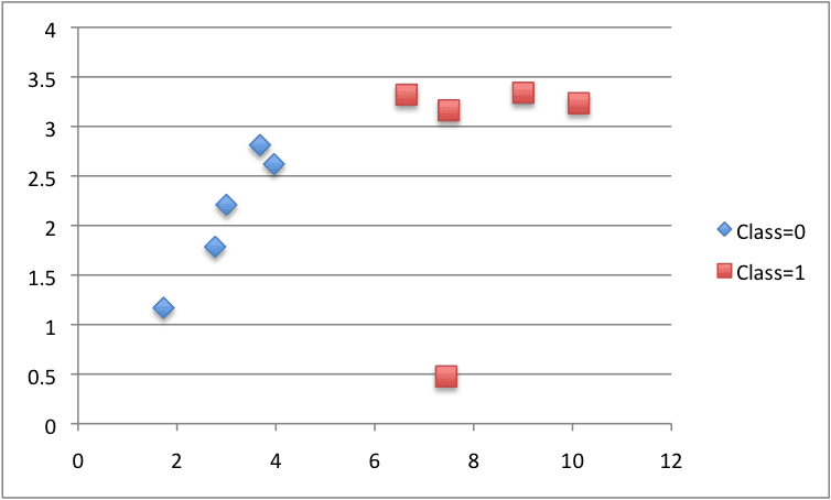
CART Contrived Dataset

The example below puts all of this together.

The get_split() function was modified to print out each split point and it’s Gini index as it was evaluated.

Running the example prints all of the Gini scores and then prints the score of best split in the dataset of X1 < 6.642 with a Gini Index of 0.0 or a perfect split.

Now that we know how to find the best split points in a dataset or list of rows, let’s see how we can use it to build out a decision tree.

3. Build a Tree

Creating the root node of the tree is easy.

We call the above get_split() function using the entire dataset.

Adding more nodes to our tree is more interesting.

Building a tree may be divided into 3 main parts:

1. Terminal Nodes.
2. Recursive Splitting.
3. Building a Tree.

3.1. Terminal Nodes

We need to decide when to stop growing a tree.

We can do that using the depth and the number of rows that the node is responsible for in the training dataset.

• Maximum Tree Depth. This is the maximum number of nodes from the root node of the tree. Once a maximum depth of the tree is met, we must stop splitting adding new nodes. Deeper trees are more complex and are more likely to overfit the training data.
• Minimum Node Records. This is the minimum number of training patterns that a given node is responsible for. Once at or below this minimum, we must stop splitting and adding new nodes. Nodes that account for too few training patterns are expected to be too specific and are likely to overfit the training data.

These two approaches will be user-specified arguments to our tree building procedure.

There is one more condition. It is possible to choose a split in which all rows belong to one group. In this case, we will be unable to continue splitting and adding child nodes as we will have no records to split on one side or another.

Now we have some ideas of when to stop growing the tree. When we do stop growing at a given point, that node is called a terminal node and is used to make a final prediction.

This is done by taking the group of rows assigned to that node and selecting the most common class value in the group. This will be used to make predictions.

Below is a function named to_terminal() that will select a class value for a group of rows. It returns the most common output value in a list of rows.

3.2. Recursive Splitting

We know how and when to create terminal nodes, now we can build our tree.

Building a decision tree involves calling the above developed get_split() function over and over again on the groups created for each node.

New nodes added to an existing node are called child nodes. A node may have zero children (a terminal node), one child (one side makes a prediction directly) or two child nodes. We will refer to the child nodes as left and right in the dictionary representation of a given node.

Once a node is created, we can create child nodes recursively on each group of data from the split by calling the same function again.

Below is a function that implements this recursive procedure. It takes a node as an argument as well as the maximum depth, minimum number of patterns in a node and the current depth of a node.

You can imagine how this might be first called passing in the root node and the depth of 1. This function is best explained in steps:

1. Firstly, the two groups of data split by the node are extracted for use and deleted from the node. As we work on these groups the node no longer requires access to these data.
2. Next, we check if either left or right group of rows is empty and if so we create a terminal node using what records we do have.
3. We then check if we have reached our maximum depth and if so we create a terminal node.
4. We then process the left child, creating a terminal node if the group of rows is too small, otherwise creating and adding the left node in a depth first fashion until the bottom of the tree is reached on this branch.
5. The right side is then processed in the same manner, as we rise back up the constructed tree to the root.

3.3. Building a Tree

We can now put all of the pieces together.

Building the tree involves creating the root node and calling the split() function that then calls itself recursively to build out the whole tree.

Below is the small build_tree() function that implements this procedure.

We can test out this whole procedure using the small dataset we contrived above.

Below is the complete example.

Also included is a small print_tree() function that recursively prints out nodes of the decision tree with one line per node. Although not as striking as a real decision tree diagram, it gives an idea of the tree structure and decisions made throughout.

We can vary the maximum depth argument as we run this example and see the effect on the printed tree.

With a maximum depth of 1 (the second parameter in the call to the build_tree() function), we can see that the tree uses the perfect split we discovered in the previous section. This is a tree with one node, also called a decision stump.

Increasing the maximum depth to 2, we are forcing the tree to make splits even when none are required. The X1 attribute is then used again by both the left and right children of the root node to split up the already perfect mix of classes.

Finally, and perversely, we can force one more level of splits with a maximum depth of 3.

These tests show that there is great opportunity to refine the implementation to avoid unnecessary splits. This is left as an extension.

Now that we can create a decision tree, let’s see how we can use it to make predictions on new data.

4. Make a Prediction

Making predictions with a decision tree involves navigating the tree with the specifically provided row of data.

Again, we can implement this using a recursive function, where the same prediction routine is called again with the left or the right child nodes, depending on how the split affects the provided data.

We must check if a child node is either a terminal value to be returned as the prediction, or if it is a dictionary node containing another level of the tree to be considered.

Below is the predict() function that implements this procedure. You can see how the index and value in a given node

You can see how the index and value in a given node is used to evaluate whether the row of provided data falls on the left or the right of the split.

We can use our contrived dataset to test this function. Below is an example that uses a hard-coded decision tree with a single node that best splits the data (a decision stump).

The example makes a prediction for each row in the dataset.

Running the example prints the correct prediction for each row, as expected.

We now know how to create a decision tree and use it to make predictions. Now, let’s apply it to a real dataset.

5. Banknote Case Study

This section applies the CART algorithm to the Bank Note dataset.

The first step is to load the dataset and convert the loaded data to numbers that we can use to calculate split points. For this we will use the helper function load_csv() to load the file and str_column_to_float() to convert string numbers to floats.

We will evaluate the algorithm using k-fold cross-validation with 5 folds. This means that 1372/5=274.4 or just over 270 records will be used in each fold. We will use the helper functions evaluate_algorithm() to evaluate the algorithm with cross-validation and accuracy_metric() to calculate the accuracy of predictions.

A new function named decision_tree() was developed to manage the application of the CART algorithm, first creating the tree from the training dataset, then using the tree to make predictions on a test dataset.

The complete example is listed below.

The example uses the max tree depth of 5 layers and the minimum number of rows per node to 10. These parameters to CART were chosen with a little experimentation, but are by no means are they optimal.

Running the example prints the average classification accuracy on each fold as well as the average performance across all folds.

You can see that CART and the chosen configuration achieved a mean classification accuracy of about 97% which is dramatically better than the Zero Rule algorithm that achieved 50% accuracy.

Extensions

This section lists extensions to this tutorial that you may wish to explore.

• Algorithm Tuning. The application of CART to the Bank Note dataset was not tuned. Experiment with different parameter values and see if you can achieve better performance.
• Cross Entropy. Another cost function for evaluating splits is cross entropy (logloss). You could implement and experiment with this alternative cost function.
• Tree Pruning. An important technique for reducing overfitting of the training dataset is to prune the trees. Investigate and implement tree pruning methods.
• Categorical Dataset. The example was designed for input data with numerical or ordinal input attributes, experiment with categorical input data and splits that may use equality instead of ranking.
• Regression. Adapt the tree for regression using a different cost function and method for creating terminal nodes.
• More Datasets. Apply the algorithm to more datasets on the UCI Machine Learning Repository.

Did you explore any of these extensions?
Share your experiences in the comments below.

Review

In this tutorial, you discovered how to implement the decision tree algorithm from scratch with Python.

Specifically, you learned:

• How to select and evaluate split points in a training dataset.
• How to recursively build a decision tree from multiple splits.
• How to apply the CART algorithm to a real world classification predictive modeling problem.

Do you have any questions?
Ask your questions in the comments below and I will do my best to answer them.

Discover How to Code Algorithms From Scratch!

No Libraries, Just Python Code.

...with step-by-step tutorials on real-world datasets

Discover how in my new Ebook:
Machine Learning Algorithms From Scratch

It covers 18 tutorials with all the code for 12 top algorithms, like:
Linear Regression, k-Nearest Neighbors, Stochastic Gradient Descent and much more...

Finally, Pull Back the Curtain on
Machine Learning Algorithms

Skip the Academics. Just Results.

See What's Inside