Classification And Regression Trees for Machine Learning

Last Updated on August 15, 2020

Decision Trees are an important type of algorithm for predictive modeling machine learning.

The classical decision tree algorithms have been around for decades and modern variations like random forest are among the most powerful techniques available.

In this post you will discover the humble decision tree algorithm known by it’s more modern name CART which stands for Classification And Regression Trees. After reading this post, you will know:

• The many names used to describe the CART algorithm for machine learning.
• The representation used by learned CART models that is actually stored on disk.
• How a CART model can be learned from training data.
• How a learned CART model can be used to make predictions on unseen data.
• Additional resources that you can use to learn more about CART and related algorithms.

If you have taken an algorithms and data structures course, it might be hard to hold you back from implementing this simple and powerful algorithm. And from there, you’re a small step away from your own implementation of Random Forests.

Kick-start your project with my new book Master Machine Learning Algorithms, including step-by-step tutorials and the Excel Spreadsheet files for all examples.

Let’s get started.

• Update Aug 2017: Fixed a typo that indicated that Gini is the count of instances for a class, should have been the proportion of instances. Also updated to show Gini weighting for evaluating the split in addition to calculating purity for child nodes.

Classification And Regression Trees for Machine Learning
Photo by Wonderlane, some rights reserved.

Decision Trees

Classification and Regression Trees or CART for short is a term introduced by Leo Breiman to refer to Decision Tree algorithms that can be used for classification or regression predictive modeling problems.

Classically, this algorithm is referred to as “decision trees”, but on some platforms like R they are referred to by the more modern term CART.

The CART algorithm provides a foundation for important algorithms like bagged decision trees, random forest and boosted decision trees.

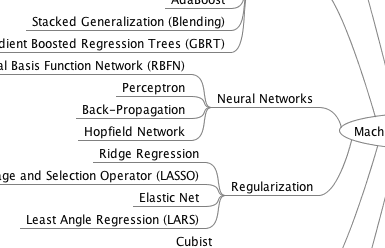
Get your FREE Algorithms Mind Map

Sample of the handy machine learning algorithms mind map.

I've created a handy mind map of 60+ algorithms organized by type.

Download it, print it and use it. 

CART Model Representation

The representation for the CART model is a binary tree.

This is your binary tree from algorithms and data structures, nothing too fancy. Each root node represents a single input variable (x) and a split point on that variable (assuming the variable is numeric).

The leaf nodes of the tree contain an output variable (y) which is used to make a prediction.

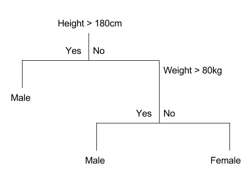
Given a dataset with two inputs (x) of height in centimeters and weight in kilograms the output of sex as male or female, below is a crude example of a binary decision tree (completely fictitious for demonstration purposes only).

Example Decision Tree

The tree can be stored to file as a graph or a set of rules. For example, below is the above decision tree as a set of rules.

With the binary tree representation of the CART model described above, making predictions is relatively straightforward.

Given a new input, the tree is traversed by evaluating the specific input started at the root node of the tree.

A learned binary tree is actually a partitioning of the input space. You can think of each input variable as a dimension on a p-dimensional space. The decision tree split this up into rectangles (when p=2 input variables) or some kind of hyper-rectangles with more inputs.

New data is filtered through the tree and lands in one of the rectangles and the output value for that rectangle is the prediction made by the model. This gives you some feeling for the type of decisions that a CART model is capable of making, e.g. boxy decision boundaries.

For example, given the input of [height = 160 cm, weight = 65 kg], we would traverse the above tree as follows:

Learn a CART Model From Data

Creating a CART model involves selecting input variables and split points on those variables until a suitable tree is constructed.

The selection of which input variable to use and the specific split or cut-point is chosen using a greedy algorithm to minimize a cost function. Tree construction ends using a predefined stopping criterion, such as a minimum number of training instances assigned to each leaf node of the tree.

Greedy Splitting

Creating a binary decision tree is actually a process of dividing up the input space. A greedy approach is used to divide the space called recursive binary splitting.

This is a numerical procedure where all the values are lined up and different split points are tried and tested using a cost function. The split with the best cost (lowest cost because we minimize cost) is selected.

All input variables and all possible split points are evaluated and chosen in a greedy manner (e.g. the very best split point is chosen each time).

For regression predictive modeling problems the cost function that is minimized to choose split points is the sum squared error across all training samples that fall within the rectangle:

sum(y – prediction)^2

Where y is the output for the training sample and prediction is the predicted output for the rectangle.

For classification the Gini index function is used which provides an indication of how “pure” the leaf nodes are (how mixed the training data assigned to each node is).

G = sum(pk * (1 – pk))

Where G is the Gini index over all classes, pk are the proportion of training instances with class k in the rectangle of interest. A node that has all classes of the same type (perfect class purity) will have G=0, where as a G that has a 50-50 split of classes for a binary classification problem (worst purity) will have a G=0.5.

For a binary classification problem, this can be re-written as:

G = 2 * p1 * p2
or
G = 1 – (p1^2 + p2^2)

The Gini index calculation for each node is weighted by the total number of instances in the parent node. The Gini score for a chosen split point in a binary classification problem is therefore calculated as follows:

G = ((1 – (g1_1^2 + g1_2^2)) * (ng1/n)) + ((1 – (g2_1^2 + g2_2^2)) * (ng2/n))

Where G is the Gini index for the split point, g1_1 is the proportion of instances in group 1 for class 1, g1_2 for class 2, g2_1 for group 2 and class 1, g2_2 group 2 class 2, ng1 and ng2 are the total number of instances in group 1 and 2 and n are the total number of instances we are trying to group from the parent node.

Stopping Criterion

The recursive binary splitting procedure described above needs to know when to stop splitting as it works its way down the tree with the training data.

The most common stopping procedure is to use a minimum count on the number of training instances assigned to each leaf node. If the count is less than some minimum then the split is not accepted and the node is taken as a final leaf node.

The count of training members is tuned to the dataset, e.g. 5 or 10. It defines how specific to the training data the tree will be. Too specific (e.g. a count of 1) and the tree will overfit the training data and likely have poor performance on the test set.

Pruning The Tree

The stopping criterion is important as it strongly influences the performance of your tree. You can use pruning after learning your tree to further lift performance.

The complexity of a decision tree is defined as the number of splits in the tree. Simpler trees are preferred. They are easy to understand (you can print them out and show them to subject matter experts), and they are less likely to overfit your data.

The fastest and simplest pruning method is to work through each leaf node in the tree and evaluate the effect of removing it using a hold-out test set. Leaf nodes are removed only if it results in a drop in the overall cost function on the entire test set. You stop removing nodes when no further improvements can be made.

More sophisticated pruning methods can be used such as cost complexity pruning (also called weakest link pruning) where a learning parameter (alpha) is used to weigh whether nodes can be removed based on the size of the sub-tree.

Recursive Binary Splitting for Decision Trees
Photo by Paul L Dineen, some rights reserved.

Data Preparation for CART

CART does not require any special data preparation other than a good representation of the problem.

Further Reading

This section lists some resources that you can refer to if you are looking to go deeper with CART.

• Classification and Regression Trees

Below are some good machine learning texts that describe the CART algorithm from a machine learning perspective.

• An Introduction to Statistical Learning: with Applications in R, Chapter 8
• Applied Predictive Modeling, Chapter 8 and 14
• Data Mining: Practical Machine Learning Tools and Techniques, chapter 6.

Summary

In this post you have discovered the Classification And Regression Trees (CART) for machine learning. You learned:

• The classical name Decision Tree and the more Modern name CART for the algorithm.
• The representation used for CART is a binary tree.
• Predictions are made with CART by traversing the binary tree given a new input record.
• The tree is learned using a greedy algorithm on the training data to pick splits in the tree.
• Stopping criteria define how much tree learns and pruning can be used to improve a learned tree.

Do you have any questions about CART or this post?
Ask in the comments and I will do my best to answer.

Discover How Machine Learning Algorithms Work!

See How Algorithms Work in Minutes

...with just arithmetic and simple examples

Discover how in my new Ebook:
Master Machine Learning Algorithms

It covers explanations and examples of 10 top algorithms, like:
Linear Regression, k-Nearest Neighbors, Support Vector Machines and much more...

Finally, Pull Back the Curtain on
Machine Learning Algorithms

Skip the Academics. Just Results.

See What's Inside