Too many epochs can lead to overfitting of the training dataset, whereas too few may result in an underfit model. Early stopping is a method that allows you to specify an arbitrary large number of training epochs and stop training once the model performance stops improving on a hold out validation dataset.
In this tutorial, you will discover the Keras API for adding early stopping to overfit deep learning neural network models.
After completing this tutorial, you will know:
How to monitor the performance of a model during training using the Keras API.
How to create and configure early stopping and model checkpoint callbacks using the Keras API.
How to reduce overfitting by adding an early stopping to an existing model.
Kick-start your project with my new book Better Deep Learning, including step-by-step tutorials and the Python source code files for all examples.
Let’s get started.
Updated Oct/2019: Updated for Keras 2.3 and TensorFlow 2.0.
How to Stop Training Deep Neural Networks At the Right Time With Using Early Stopping Photo by Ian D. Keating, some rights reserved.
Tutorial Overview
This tutorial is divided into six parts; they are:
Using Callbacks in Keras
Evaluating a Validation Dataset
Monitoring Model Performance
Early Stopping in Keras
Checkpointing in Keras
Early Stopping Case Study
Using Callbacks in Keras
Callbacks provide a way to execute code and interact with the training model process automatically.
Callbacks can be provided to the fit() function via the “callbacks” argument.
First, callbacks must be instantiated.
1
2
...
cb=Callback(...)
Then, one or more callbacks that you intend to use must be added to a Python list.
1
2
...
cb_list=[cb,...]
Finally, the list of callbacks is provided to the callback argument when fitting the model.
1
2
...
model.fit(...,callbacks=cb_list)
Evaluating a Validation Dataset in Keras
Early stopping requires that a validation dataset is evaluated during training.
This can be achieved by specifying the validation dataset to the fit() function when training your model.
There are two ways of doing this.
The first involves you manually splitting your training data into a train and validation dataset and specifying the validation dataset to the fit() function via the validation_data argument. For example:
Alternately, the fit() function can automatically split your training dataset into train and validation sets based on a percentage split specified via the validation_split argument.
The validation_split is a value between 0 and 1 and defines the percentage amount of the training dataset to use for the validation dataset. For example:
1
2
...
model.fit(train_X,train_y,validation_split=0.3)
In both cases, the model is not trained on the validation dataset. Instead, the model is evaluated on the validation dataset at the end of each training epoch.
Want Better Results with Deep Learning?
Take my free 7-day email crash course now (with sample code).
Click to sign-up and also get a free PDF Ebook version of the course.
To callbacks, this is made available via the name “loss.”
If a validation dataset is specified to the fit() function via the validation_data or validation_split arguments, then the loss on the validation dataset will be made available via the name “val_loss.”
Additional metrics can be monitored during the training of the model.
They can be specified when compiling the model via the “metrics” argument to the compile function. This argument takes a Python list of known metric functions, such as ‘mse‘ for mean squared error and ‘accuracy‘ for accuracy. For example:
1
2
...
model.compile(...,metrics=['accuracy'])
If additional metrics are monitored during training, they are also available to the callbacks via the same name, such as ‘accuracy‘ for accuracy on the training dataset and ‘val_accuracy‘ for the accuracy on the validation dataset. Or, ‘mse‘ for mean squared error on the training dataset and ‘val_mse‘ on the validation dataset.
Early Stopping in Keras
Keras supports the early stopping of training via a callback called EarlyStopping.
This callback allows you to specify the performance measure to monitor, the trigger, and once triggered, it will stop the training process.
The EarlyStopping callback is configured when instantiated via arguments.
The “monitor” allows you to specify the performance measure to monitor in order to end training. Recall from the previous section that the calculation of measures on the validation dataset will have the ‘val_‘ prefix, such as ‘val_loss‘ for the loss on the validation dataset.
1
es=EarlyStopping(monitor='val_loss')
Based on the choice of performance measure, the “mode” argument will need to be specified as whether the objective of the chosen metric is to increase (maximize or ‘max‘) or to decrease (minimize or ‘min‘).
For example, we would seek a minimum for validation loss and a minimum for validation mean squared error, whereas we would seek a maximum for validation accuracy.
1
es=EarlyStopping(monitor='val_loss',mode='min')
By default, mode is set to ‘auto‘ and knows that you want to minimize loss or maximize accuracy.
That is all that is needed for the simplest form of early stopping. Training will stop when the chosen performance measure stops improving. To discover the training epoch on which training was stopped, the “verbose” argument can be set to 1. Once stopped, the callback will print the epoch number.
Often, the first sign of no further improvement may not be the best time to stop training. This is because the model may coast into a plateau of no improvement or even get slightly worse before getting much better.
We can account for this by adding a delay to the trigger in terms of the number of epochs on which we would like to see no improvement. This can be done by setting the “patience” argument.
The exact amount of patience will vary between models and problems. Reviewing plots of your performance measure can be very useful to get an idea of how noisy the optimization process for your model on your data may be.
By default, any change in the performance measure, no matter how fractional, will be considered an improvement. You may want to consider an improvement that is a specific increment, such as 1 unit for mean squared error or 1% for accuracy. This can be specified via the “min_delta” argument.
Finally, it may be desirable to only stop training if performance stays above or below a given threshold or baseline. For example, if you have familiarity with the training of the model (e.g. learning curves) and know that once a validation loss of a given value is achieved that there is no point in continuing training. This can be specified by setting the “baseline” argument.
This might be more useful when fine tuning a model, after the initial wild fluctuations in the performance measure seen in the early stages of training a new model are past.
The EarlyStopping callback will stop training once triggered, but the model at the end of training may not be the model with best performance on the validation dataset.
An additional callback is required that will save the best model observed during training for later use. This is the ModelCheckpoint callback.
The ModelCheckpoint callback is flexible in the way it can be used, but in this case we will use it only to save the best model observed during training as defined by a chosen performance measure on the validation dataset.
Saving and loading models requires that HDF5 support has been installed on your workstation. For example, using the pip Python installer, this can be achieved as follows:
The callback will save the model to file, which requires that a path and filename be specified via the first argument.
1
mc=ModelCheckpoint('best_model.h5')
The preferred loss function to be monitored can be specified via the monitor argument, in the same way as the EarlyStopping callback. For example, loss on the validation dataset (the default).
Also, as with the EarlyStopping callback, we must specify the “mode” as either minimizing or maximizing the performance measure. Again, the default is ‘auto,’ which is aware of the standard performance measures.
Finally, we are interested in only the very best model observed during training, rather than the best compared to the previous epoch, which might not be the best overall if training is noisy. This can be achieved by setting the “save_best_only” argument to True.
That is all that is needed to ensure the model with the best performance is saved when using early stopping, or in general.
It may be interesting to know the value of the performance measure and at what epoch the model was saved. This can be printed by the callback by setting the “verbose” argument to “1“.
The saved model can then be loaded and evaluated any time by calling the load_model() function.
1
2
3
# load a saved model
from keras.models import load_model
saved_model=load_model('best_model.h5')
Now that we know how to use the early stopping and model checkpoint APIs, let’s look at a worked example.
Early Stopping Case Study
In this section, we will demonstrate how to use early stopping to reduce overfitting of an MLP on a simple binary classification problem.
This example provides a template for applying early stopping to your own neural network for classification and regression problems.
Binary Classification Problem
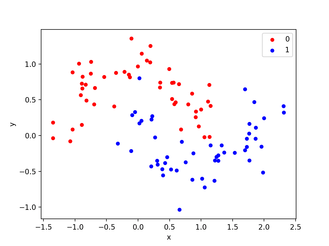
We will use a standard binary classification problem that defines two semi-circles of observations, one semi-circle for each class.
Each observation has two input variables with the same scale and a class output value of either 0 or 1. This dataset is called the “moons” dataset because of the shape of the observations in each class when plotted.
We can use the make_moons() function to generate observations from this problem. We will add noise to the data and seed the random number generator so that the same samples are generated each time the code is run.
We can plot the dataset where the two variables are taken as x and y coordinates on a graph and the class value is taken as the color of the observation.
The complete example of generating the dataset and plotting it is listed below.
Running the example creates a scatter plot showing the semi-circle or moon shape of the observations in each class. We can see the noise in the dispersal of the points making the moons less obvious.
Scatter Plot of Moons Dataset With Color Showing the Class Value of Each Sample
This is a good test problem because the classes cannot be separated by a line, e.g. are not linearly separable, requiring a nonlinear method such as a neural network to address.
We have only generated 100 samples, which is small for a neural network, providing the opportunity to overfit the training dataset and have higher error on the test dataset: a good case for using regularization. Further, the samples have noise, giving the model an opportunity to learn aspects of the samples that don’t generalize.
Overfit Multilayer Perceptron
We can develop an MLP model to address this binary classification problem.
The model will have one hidden layer with more nodes than may be required to solve this problem, providing an opportunity to overfit. We will also train the model for longer than is required to ensure the model overfits.
Before we define the model, we will split the dataset into train and test sets, using 30 examples to train the model and 70 to evaluate the fit model’s performance.
The hidden layer uses 500 nodes and the rectified linear activation function. A sigmoid activation function is used in the output layer in order to predict class values of 0 or 1. The model is optimized using the binary cross entropy loss function, suitable for binary classification problems and the efficient Adam version of gradient descent.
The defined model is then fit on the training data for 4,000 epochs and the default batch size of 32.
We will also use the test dataset as a validation dataset. This is just a simplification for this example. In practice, you would split the training set into train and validation and also hold back a test set for final model evaluation.
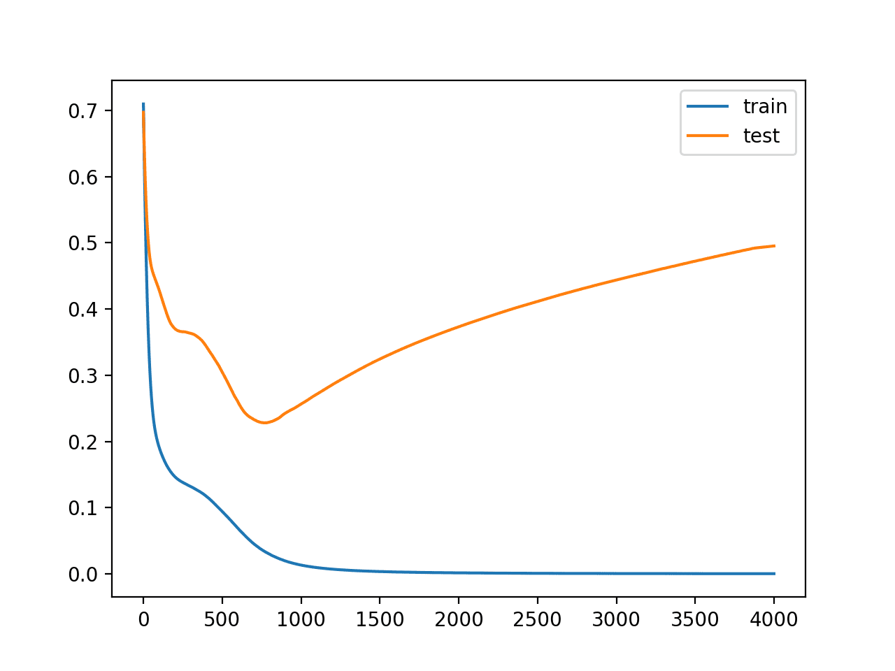
Finally, we will plot the loss of the model on both the train and test set each epoch.
If the model does indeed overfit the training dataset, we would expect the line plot of loss (and accuracy) on the training set to continue to increase and the test set to rise and then fall again as the model learns statistical noise in the training dataset.
Running the example reports the model performance on the train and test datasets.
We can see that the model has better performance on the training dataset than the test dataset, one possible sign of overfitting.
Note: Your results may vary given the stochastic nature of the algorithm or evaluation procedure, or differences in numerical precision. Consider running the example a few times and compare the average outcome.
Because the model is severely overfit, we generally would not expect much, if any, variance in the accuracy across repeated runs of the model on the same dataset.
1
Train: 1.000, Test: 0.914
A figure is created showing line plots of the model loss on the train and test sets.
We can see that expected shape of an overfit model where test accuracy increases to a point and then begins to decrease again.
Reviewing the figure, we can also see flat spots in the ups and downs in the validation loss. Any early stopping will have to account for these behaviors. We would also expect that a good time to stop training might be around epoch 800.
Line Plots of Loss on Train and Test Datasets While Training Showing an Overfit Model
Overfit MLP With Early Stopping
We can update the example and add very simple early stopping.
As soon as the loss of the model begins to increase on the test dataset, we will stop training.
Running the example reports the model performance on the train and test datasets.
Note: Your results may vary given the stochastic nature of the algorithm or evaluation procedure, or differences in numerical precision. Consider running the example a few times and compare the average outcome.
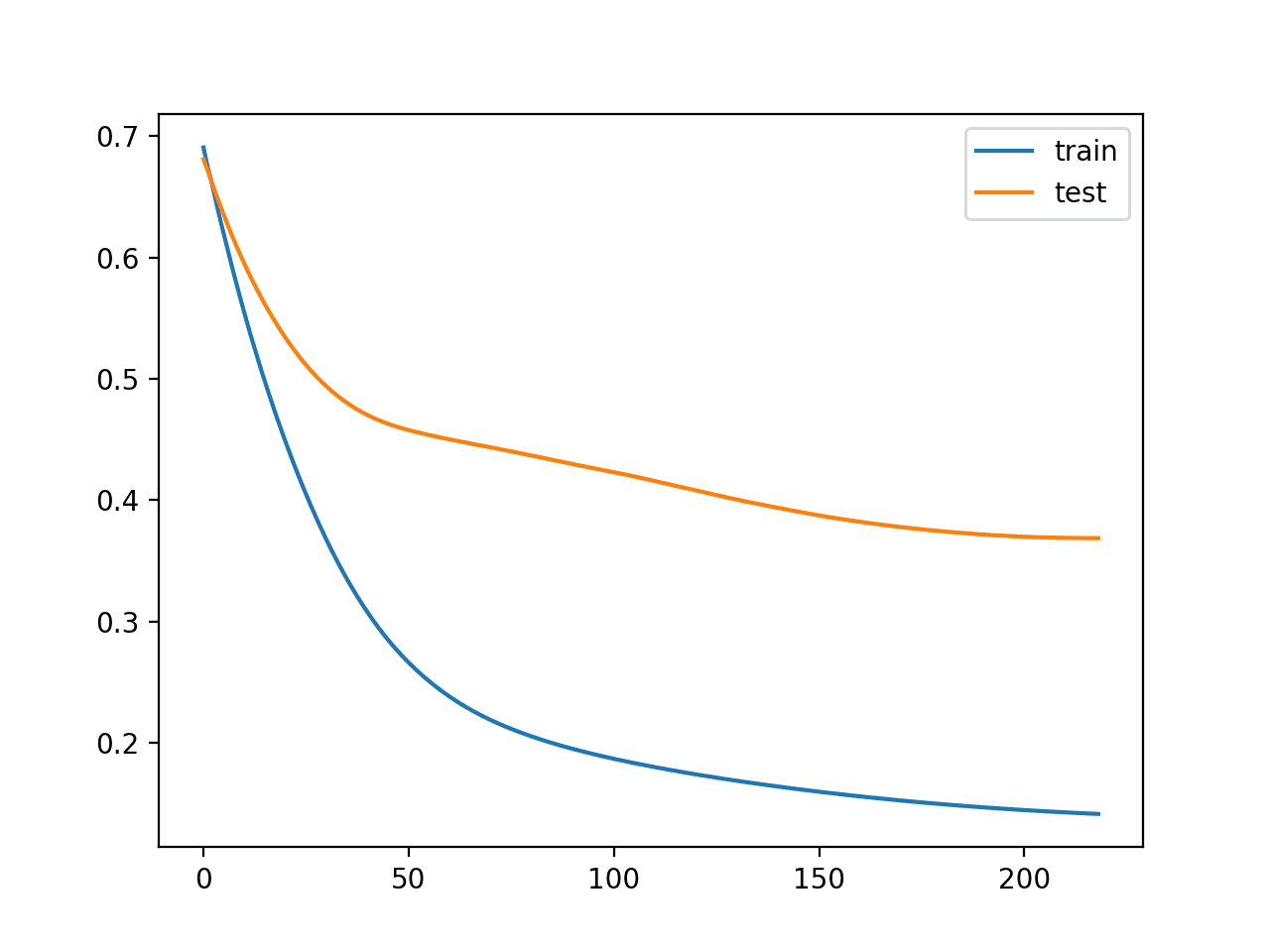
We can also see that the callback stopped training at epoch 200. This is too early as we would expect an early stop to be around epoch 800. This is also highlighted by the classification accuracy on both the train and test sets, which is worse than no early stopping.
1
2
Epoch 00219: early stopping
Train: 0.967, Test: 0.814
Reviewing the line plot of train and test loss, we can indeed see that training was stopped at the point when validation loss began to plateau for the first time.
Line Plot of Train and Test Loss During Training With Simple Early Stopping
We can improve the trigger for early stopping by waiting a while before stopping.
This can be achieved by setting the “patience” argument.
In this case, we will wait 200 epochs before training is stopped. Specifically, this means that we will allow training to continue for up to an additional 200 epochs after the point that validation loss started to degrade, giving the training process an opportunity to get across flat spots or find some additional improvement.
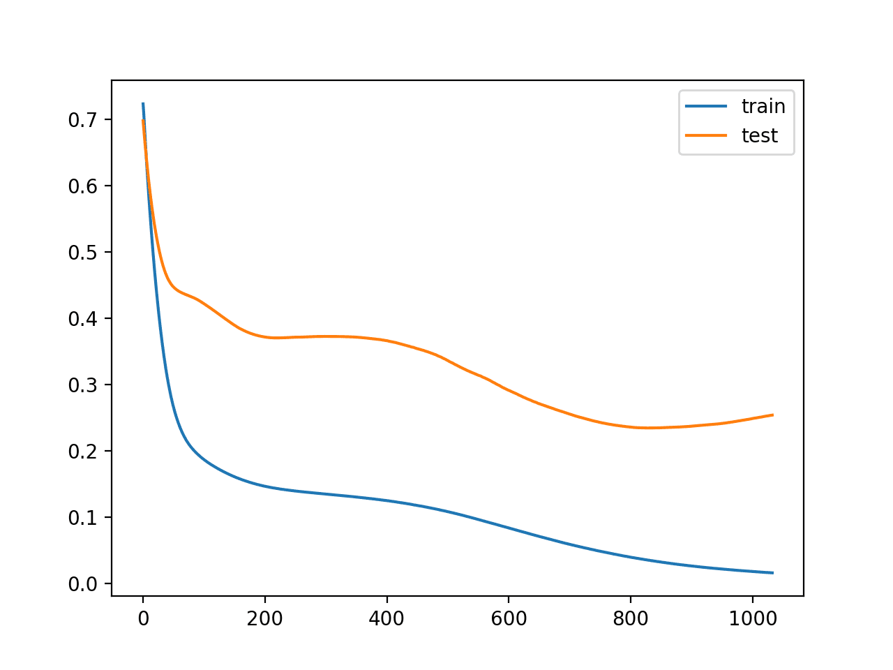
Running the example, we can see that training was stopped much later, in this case after epoch 1,000.
Note: Your results may vary given the stochastic nature of the algorithm or evaluation procedure, or differences in numerical precision. Consider running the example a few times and compare the average outcome.
We can also see that the performance on the test dataset is better than not using any early stopping.
1
2
Epoch 01033: early stopping
Train: 1.000, Test: 0.943
Reviewing the line plot of loss during training, we can see that the patience allowed the training to progress past some small flat and bad spots.
Line Plot of Train and Test Loss During Training With Patient Early Stopping
We can also see that test loss started to increase again in the last approximately 100 epochs.
This means that although the performance of the model has improved, we may not have the best performing or most stable model at the end of training. We can address this by using a ModelChecckpoint callback.
In this case, we are interested in saving the model with the best accuracy on the test dataset. We could also seek the model with the best loss on the test dataset, but this may or may not correspond to the model with the best accuracy.
This highlights an important concept in model selection. The notion of the “best” model during training may conflict when evaluated using different performance measures. Try to choose models based on the metric by which they will be evaluated and presented in the domain. In a balanced binary classification problem, this will most likely be classification accuracy. Therefore, we will use accuracy on the validation in the ModelCheckpoint callback to save the best model observed during training.
During training, the entire model will be saved to the file “best_model.h5” only when accuracy on the validation dataset improves overall across the entire training process. A verbose output will also inform us as to the epoch and accuracy value each time the model is saved to the same file (e.g. overwritten).
This new additional callback can be added to the list of callbacks when calling the fit() function.
Running the example, we can see the verbose output from the ModelCheckpoint callback for both when a new best model is saved and from when no improvement was observed.
We can see that the best model was observed at epoch 879 during this run.
Note: Your results may vary given the stochastic nature of the algorithm or evaluation procedure, or differences in numerical precision. Consider running the example a few times and compare the average outcome.
Again, we can see that early stopping continued patiently until after epoch 1,000. Note that epoch 880 + a patience of 200 is not epoch 1044. Recall that early stopping is monitoring loss on the validation dataset and that the model checkpoint is saving models based on accuracy. As such, the patience of early stopping started at an epoch other than 880.
1
2
3
4
5
6
7
8
9
10
...
Epoch 00878: val_acc did not improve from 0.92857
Epoch 00879: val_acc improved from 0.92857 to 0.94286, saving model to best_model.h5
Epoch 00880: val_acc did not improve from 0.94286
...
Epoch 01042: val_acc did not improve from 0.94286
Epoch 01043: val_acc did not improve from 0.94286
Epoch 01044: val_acc did not improve from 0.94286
Epoch 01044: early stopping
Train: 1.000, Test: 0.943
In this case, we don’t see any further improvement in model accuracy on the test dataset. Nevertheless, we have followed a good practice.
Why not monitor validation accuracy for early stopping?
This is a good question. The main reason is that accuracy is a coarse measure of model performance during training and that loss provides more nuance when using early stopping with classification problems. The same measure may be used for early stopping and model checkpointing in the case of regression, such as mean squared error.
Extensions
This section lists some ideas for extending the tutorial that you may wish to explore.
Use Accuracy. Update the example to monitor accuracy on the test dataset rather than loss, and plot learning curves showing accuracy.
Use True Validation Set. Update the example to split the training set into train and validation sets, then evaluate the model on the test dataset.
Regression Example. Create a new example of using early stopping to address overfitting on a simple regression problem and monitoring mean squared error.
If you explore any of these extensions, I’d love to know.
Further Reading
This section provides more resources on the topic if you are looking to go deeper.
Is this process of early stopping should be done after we selected the suitable architecture for the neural network (Maybe using cross-validation scores of different architectures.)?
Thank you for the tutorial. Big fan of this site 🙂
Hi Jason, this is stupendous article. Congratulations.
Still reading and has a lot to get from him.
In november i posted in another post of yours about checkpoints, my main objective at that time ( and still is) is to do hyperparam optimization with checkpoints.
Do you think the Early Stopping approach can achieve this by Stopping->Reloading->Compiling->Continue Training->Hyperparam change->Stopping->So on …
But, to use Early Stopping, isnt the same of checkpoint/reloading/recompiling and running ?
My point is: I wanna to be able to reload the same model and continue training until min loss AND change model hyperparams (Archs, Batch Size, Epoch Num) and retrain it with the same data split as before (or same dataset, as if i were forced to change splitting due to different batch size).
The Whole point maybe is: Is there in Keras a proxy to hyperparam tuning, aside that one of sklearn (that doesnt work too well with Keras checkpoints) ?
I use early stopping for LSTM forecasting. when I ran training for the first time, early stopping stopped at Epoch 20, and when I run it it stopped for the second time in Epoch 17. It was always different every time. can you explain why that happened?
Thanks for the excellent post and helping in understanding DL related topics. I have a question.
When we use ModelCheckpoint whether only the weights would be saved or the complete model (along with the model architecture)
Whenever I try to save the model and load it directly in a different program it throws up and error (Error details will post soon).
saved_model = load_model(‘best_model.h5’)
So what I had to follow the below approach:
1. First build the model architecture .
2. Then load the saved weight (or model, I am using the .h5 file saved using ModelCheckpoint)
Is this the right approach? I can share the github link so that you can have a look at my code if everything is fine.
Hi Jason, thank you very much for your post, it is very useful. But in my model, I can not use the ModelCheckPoints, the error says the loss is unknown, so I guess the Model checkpoints is not suitable for the model with customized loss function?
Hi Jason, Thanks for the clarification. As of now I am doing it in a single program. I will write a separate code to create the model architecture again.
I have a question. Let’s say I have gone through the full round of hyperparameter tuning with kfold cross validation.. and settle on an architecture, parameters, etc. I am ready to use the final model externally. Would I just take one of the trained models from one of the folds? Or.. Would you train the final model on all of the data? With a validation set, you have an indication of when it starts to overfit, while training with all of the data means the models gets to see more data.
The problem is if you train on all of the data.. it’s hard to know at what epoch to stop training.
Hi Jason,
I was wondering if there there is any hard and bound rule to use minimization of validation loss for early stopping. Say, I use ‘validation accuracy’ i.e. if the validation accuracy stays same or starts decreasing,then I stop training my model. What are the pros and cons of this approach in your opinion?
Hello Jason, I don’t understand if early stopping with patience of 4 (for example) will stop training when val_loss_i > val_loss_i -1 > val_loss_i -2 > val_loss_i -3 (a sequence of loss increasing)
Or will stop training when val_loss_i > min_overall_val_loss & val_loss_i-1 > min_overall_val_loss & val_loss_i-2 > min_overall_val_loss & val_loss_i-3 > min_overall_val_loss (a sequence that independently do not perform better than the overall min loss)
Sorry I can explain better: do the early stopping mecanism takes into account the minimum overall loss (from all previous epochs) ? Or just takes into account the current loss until the loss of the current epoch – patience ?
Thank you for all your amazing notes. I have a question regarding training testing data split. I want to use training, testing and validation data sets. I also want to have a random split for training and testing data sets for each epoch. Is it possible in Keras?
Or in simpler words can I do like this:
1. Split data into training and testing
2. Split the training data to training and validation. (So finally I have three sets, testing kept aside for the end)
3. Now fit a model for training data, use validation data and predict and get the model accuracy
4. If model accuracy is less than some required number go back to step to step 3 and re shuffle and get a new combination of another random training and validation datasets. Use the previous model and weights, improvise this or increment the weights from this state
5. Do this till a decent accuracy with validation is achieved
6. Then use the test data to get the final accuracy numbers
My main questions are , is this effective way of doing it? and are the weights saved when I use the fit() again, by which I mean are the weights tuned from the previous existing value everytime I use fit() command?
Thank you again Jason.
I did search for those on your blog. Didn’t get a direct answer for those questions. I guess your answers helped me to get one. Will implement this and see how it turns out. Thanks a lot for the tons of information in your blogs.
Please check the script below if I have missed anything.
Standardize the input and output data and
1. Initialize model (compile)
2. fit model
3. save model
In loop
4. Load the saved model
5. shuffle data between training and validation sets
6. model_int.fit(X_train, Y_train, epochs = 1,batch_size = 10, verbose = 1)
7. model_int.save(‘intermediate_model.h5’)
8. Predict Y using validation X data
9. Compare predicted Y data and actual Y data
10. Decide whether to back to step 4 or end based on step 7’s output.
Did I miss anything? Also saving in step 6, does it save the last batch model or the model a result of all the batches? Or should I run with batch size 1 and save after every batch and re iterate from there ?
I fit it with different sets of training and validation data sets. I keep aside a part of the data for final testing which I call test set. Then in the remaining instead of using the same training set I use different combinations of training and testing sets until the prediction shows good metrics. Once it is, I use the validation set to see the final metrics.
Hi,
I was trying to stop the model early based on the baseline. I am not sure what i am missing but, with the below command to monitor the validation loss is not working. I also tried with patience even that is not working. The model’s initial validation loss is around 21.
that might be because the baseline parameter is explained incorrectly in the article. Rather then stopping if the model reaches the value, it’s the opposite: the model stops if it does NOT reach that value, as can be seen in the keras documentation. I think the patience parameter controlls how many epochs the model has to reach the baseline before stopping.
Many thanks for all the effort you’ve put into this page, this article is one of many that I have found really helpful.
I have some trouble deciding how many epochs I should include in a final model. When deciding on the optimal configuration of my model I used early stopping to prevent the model from overfitting. When creating a final model I want to train on all the available data, so presumably I cannot apply early stopping when generating the final models.
Do you have any suggestions as to how one should decide on the number of epochs to go through when training a final model? Is it reasonable to use number of epochs at which the early stopping method stopped the training when I was configuring the model?
In the case of binary classification, I sometimes run into the scenario where validation loss starts to increase while the validation accuracy is still improving (Test accuracy also improves). I think this is because the model is still improving in predicting the labels, even though the actual loss value is getting bigger.
Can I use the model that has bigger validation accuracy (also better test accuracy) but bigger validation loss? Since our final goal is to have better prediction of labels, why do we care about increasing in loss?
Thanks for the article. When using val_acc in the Earlystopping param, it theoretically saves a model out with the model corresponding to the highest validation accuracy epoch. However, when I use the model to predict against my validation set as a check, the accuracies do not align. My model architechture uses transfer learning on NasNet.
restore_best_weights: Whether to restore model weights from the epoch with the best value of the monitored quantity. If False, the model weights obtained at the last step of training are used.
Just to let you know that there is an issue regarding the restore_best_weights option in EarlyStopping when the training is not stopped by the trigger but the total number of epochs.
First of all – Jason, thank you Sir! Amazing resources you share, as always.
@ James, i saw this as well and my take is that by using the ModelCheckpoint you get the save the best model on the fly as opposed to the Earlystopping where you need to do it separately, so when your machine crashes the model is gone. So my take is to use both to save best model and save resouces… – ?
One doubt I have regarding the data-split: are the train_X and train_y data used in the two different split approaches the same?
In
model.fit(train_X, train_y, validation_data=(val_x, val_y)), train_X and train_y should be the data used for tuning the weights and bias of the network, i.e., the first 30 rows of data in the example.
However, in
model.fit(train_X, train_y, validation_split=0.3), I guess the data we fed into the training should be the entire data set, i.e., all of the 100 samples we created in the example. Therefore, to use validation_split in the above example, the corresponding code is:
model.fit(X, y, validation_split=0.3)
I found out that keras’s early stopping cannot monitor the training loss. Do you think it will be useful if we can monitor and stop the training without the need of validation set? There could be scenario where no hyperparameter tuning is required, therefore validation set is unnecessary.
Hi Jason! Thank you for your helpful sharing. I really appreciate your work.
I just have a question. About the regression task with loss = mean_squared_error, what factors should we need to monitor with EarlyStoping (val_loss or val_mse or …)?
I do not understand this, why val_loss but not val_mse, or, why val_mse but not val_loss….?
Hi Jason, I really appreciate your work and thank you for posting such detailed tutorials. I have a question regarding the use of early stopping & model checkpoint:
I know it is ok to use your full training data to train and your test data as validation data after your model is in production (i.e, hyperparameters are tuned and model is optimized using a separate validation set already). But I am assuming using Early Stopping & Model Checkpoint on your test data leads to train-test data contamination since it has a regularization effect.
I couldn’t find a clear explanation regarding this. I would like to make sure using test data in production along with early stopping is not good in practice. But on the other hand, making the best out of your test data sounds a good idea to me, but I am not sure using Early Stopping is kind of cheating since it has a regularization effect.
Please let me know your opinion on this. Thank you in advance!
For my problem, the k-fold cv and/grid search is not really useful since data is large. When I use small epoch and big batch_sizes the difference between results almost indistinguishable. Thank you anyways!
Hi Jason,
In case of using monitor=”val_accuracy”,
is it ok to specify either patience or min_delta?
or both can be given?
In case of using min_delta say 1% for accuracy we don’t have to worry about changing patience for different values of epochs right, correct me please, Thanks
I have one question: why we need the underscore “_” before getting the accuracy score of the evaluation function:
EX: _, train_acc = model.evaluate(trainX, trainy, verbose=0)
Dear Jason,
I am grateful for the useful tutorial.
I would like to know how to use early stopping for regression.
If you have any tutorial post for using early stopping in regression, please let me know the link.
Best
Mary
Suppose I have a total of 5 epochs to make and I had a training that stopped at epoch 04 (and I have the model states at epoch 03: weights-03-0.7994.hdf5) and I would like to start the trainig again at epoch 04. Is my next code?
Hey thank you for your good description. I am trying to do early stopping with a AC GAN. Can you tell me what to do because in your tut about GAN you never used model fit
Thank you very much! Your work is something I constantly go to for reference. Thank you for all your hard work in providing great help. Appreciate the machinelearningmastery very much.
Jason, thank you for the clear explanation. These examples of yours really help me developing my algorithms and I should add that this website has been my go to knowledge base on machine learning, so thanks again for it.
My thought is, cross validation seems like an overkill if I already utilize early stopping for the simple fact that it kind of maximizes my algorithm’s learning capacity. Am I right thinking that or using cross validation on top of early stopping has its benefits?
No. They are for different purposes. Early stopping is to stop wasting time and energy to something we can’t do better. For example, you don’t want to study 10 more hours if you know you already got 99% in the exam. Cross validation is to build a model with different data/parameter and make sure you are not by luck. Same metaphor, you test a student three times with different exam questions to make sure she can score 99% every time and she actually knows it.
In my case, I built an angorithm that takes an image as input and outputs binary image of the same image. How can I configure this in a way that someone else uses my algorithm with their own images and get a result instantly without having to train it everytime?
In other words how can I convert my trained model to a basic software that takes an input and produces and output?
If you mean particular details on how to package your machine learning function into a larger software, there can be too much things to cover. I would suggest you to checkout some books on MLOps, for example.
Thank you for your adorable article. I found my test accuracy is almost always higher than the train accuracy, and my test loss is lower than the train loss. Do you know what may cause it ? I trained Mel-frequency cepstral coefficients (MFCCs) data. The input shape is (10000, 40, 162), and output is (10000, 2). The aim is to distiguish two type instruments signal from it. I doubt if it because my sample is too small, or I used a wrong model? My model is LSTM+FC(Fully connected).
Can’t tell what caused it but you can check if you see the same for multiple runs (i.e., begin from different random state of the network). It doesn’t look like the sample is too small in your case.
Hello Lana…A key consideration is the training and testing split percentage. If your testing percentage is not sufficiently large the testing accuracy will be higher than the training accuracy.
Another consideration would be the relative number of samples to the number of features. It may be the case that you need to increase the number of samples.
I’ve seen some articles suggesting that, aside from dropout/etc, that train and validation loss should be comparable, up to the point where test starts going up. In a way this makes sense, because the very next new input in production could look a lot like the training or the validation set, so having similar loss makes sense — its not any more (or less) accurate for any input that comes along.
However, your example (and others!) seem to indicate “just keep going” until validation loss starts appreciably increasing. Your example has training loss much lower than validation loss. The model is much more accurate on training-like input and the validation-like input is the worst case. At the end of the day, maybe that’s OK, but I’m wrestling with the idea of a model that might be working much better on some inputs than expected — as in that’s a bias of sorts. Thoughts?
Thanks James,
Sorry, can you help me understand the connection of how-long-to-train with dimensionality reduction? The example in this “early stopping” article has training loss much lower than validation at epoch ~800. If we had stopped at epoch 20ish, before they start to diverge, the losses would be about the same. The model can get better, but only by memorizing parts of the training data — if it happens to reduce the validation loss we’ll keep going. I guess this feels like an unspoken tradeoff that we’re getting really good at predicting almost spot-on the training data, and we’ve gotten better at the validation loss has dropped. So our generalization has improved, but we’re really much better on the training data than the validation data.
When using early stopping with restore_best_weights=True and Verbose=1
We get a message about restoring the weights from best epoch (let’s say epoch X) and that early stopping activated at epoch Y (Y > X).
Does Keras save those values (X and Y) in some variable? Is there anyway i can access them? Because i have to train my model 10 times for statistical assessement of performance, and i also wish to know at wich epoch each of those 10 iterations had the best weights and at wich epoch the early sopping activated.
in Keras, how make the model(DNN) yield a consistent result? when I run the model multiple times I get different results each time. I defined
import numpy as np
np.random.seed(0) but it could not help
import numpy as np
np.random.seed(0)
from sklearn.datasets import make_moons
from keras.models import Sequential
from keras.layers import Dense
from keras.callbacks import EarlyStopping
from matplotlib import pyplot
# generate 2d
# define model
model = Sequential()
np.random.seed(0)
model.add(Dense(256, input_dim=87, activation=’relu’))
model.add(Dense(1, activation=’sigmoid’))
model.compile(loss=’binary_crossentropy’, optimizer=’adam’, metrics=[‘accuracy’])
# simple early stopping
es = EarlyStopping(monitor=’val_loss’, mode=’min’, verbose=1)
# fit model
history = model.fit(X_train, y_train, validation_data=(X_test, y_test), epochs=15, verbose=0, callbacks=[es])
So basically it is okay to use test data in early stopping to train the model? specifically in time series, it won’t produce any data likeage, correct me if im wrong


Thanks a lot, A very clear illustration as always
Thanks, I’m glad it helped.
Hi Jason,
Is this process of early stopping should be done after we selected the suitable architecture for the neural network (Maybe using cross-validation scores of different architectures.)?
Thank you for the tutorial. Big fan of this site 🙂
Perhaps, you can start with an over-specified architecture, use weight decay and use early stopping immediately.
Wow, this is a lovely focused and lucid explanation of callbacks. Thanks for writing this Jason!
Thanks, I’m glad it helped!
Hi Jason, this is stupendous article. Congratulations.
Still reading and has a lot to get from him.
In november i posted in another post of yours about checkpoints, my main objective at that time ( and still is) is to do hyperparam optimization with checkpoints.
Do you think the Early Stopping approach can achieve this by Stopping->Reloading->Compiling->Continue Training->Hyperparam change->Stopping->So on …
??
Thank you in advance.
I generally don’t recommend using early stopping with hyperparameter tuning, it makes the process messy.
Tune parameters than add early stopping as a regularization method at the end – my best advice.
But, to use Early Stopping, isnt the same of checkpoint/reloading/recompiling and running ?
My point is: I wanna to be able to reload the same model and continue training until min loss AND change model hyperparams (Archs, Batch Size, Epoch Num) and retrain it with the same data split as before (or same dataset, as if i were forced to change splitting due to different batch size).
The Whole point maybe is: Is there in Keras a proxy to hyperparam tuning, aside that one of sklearn (that doesnt work too well with Keras checkpoints) ?
Thank you …again.
Yes, I teach writing the for-loop for parameter testing manually:
https://machinelearningmastery.com/how-to-grid-search-deep-learning-models-for-time-series-forecasting/
how about Dropout? Do the rules for weight decay also apply to Dropout?
In what way exactly?
Hi Mr. Jason
I use early stopping for LSTM forecasting. when I ran training for the first time, early stopping stopped at Epoch 20, and when I run it it stopped for the second time in Epoch 17. It was always different every time. can you explain why that happened?
my code is like this:
model = Sequential()
model.add(LSTM(4,activation=’tanh’,input_shape=(1,3),recurrent_activation= ‘hard_sigmoid’))
model.add(Dense(1))
model.compile(loss=’mean_squared_error’,optimizer=’adam’,metrics = [metrics.mae])
early_stop = EarlyStopping(monitor=’loss’, patience=2, verbose=0, mode=’min’)
model.fit(X_train,Y_train,epochs= 100 ,batch_size= 1,verbose=2, callbacks=[early_stop])
thank you
Yes, this is due to the stochastic learning algorithm.
You can learn more here:
https://machinelearningmastery.com/faq/single-faq/why-do-i-get-different-results-each-time-i-run-the-code
Hi Dr. Jason,
Thanks for the excellent post and helping in understanding DL related topics. I have a question.
When we use ModelCheckpoint whether only the weights would be saved or the complete model (along with the model architecture)
Whenever I try to save the model and load it directly in a different program it throws up and error (Error details will post soon).
saved_model = load_model(‘best_model.h5’)
So what I had to follow the below approach:
1. First build the model architecture .
2. Then load the saved weight (or model, I am using the .h5 file saved using ModelCheckpoint)
Is this the right approach? I can share the github link so that you can have a look at my code if everything is fine.
Thank you,
KK
I recommend using a function to create your model architecture again, then load the weights directly.
Hi Jason, thank you very much for your post, it is very useful. But in my model, I can not use the ModelCheckPoints, the error says the loss is unknown, so I guess the Model checkpoints is not suitable for the model with customized loss function?
Perhaps your model is mis-configured, perhaps try debugging the fault?
Hi Jason, Thanks for the clarification. As of now I am doing it in a single program. I will write a separate code to create the model architecture again.
Thank you Jason!
I have a question. Let’s say I have gone through the full round of hyperparameter tuning with kfold cross validation.. and settle on an architecture, parameters, etc. I am ready to use the final model externally. Would I just take one of the trained models from one of the folds? Or.. Would you train the final model on all of the data? With a validation set, you have an indication of when it starts to overfit, while training with all of the data means the models gets to see more data.
The problem is if you train on all of the data.. it’s hard to know at what epoch to stop training.
What would you suggest?
No, I generally recommend fitting a new final model on all available data with the best config.
If you want to use early stopping, some data will need to be held back for the validation set.
I tried to load the saved model with “load_model()” code but I got this error:
load_model() missing 1 required positional argument: ‘filepath’
can you please help me with this errror?
You must enter the path to the model file to load.
Hi Jason,
I was wondering if there there is any hard and bound rule to use minimization of validation loss for early stopping. Say, I use ‘validation accuracy’ i.e. if the validation accuracy stays same or starts decreasing,then I stop training my model. What are the pros and cons of this approach in your opinion?
Typically a rise in loss on a representative validation dataset is used as the stopping condition.
Hello Jason, I don’t understand if early stopping with patience of 4 (for example) will stop training when val_loss_i > val_loss_i -1 > val_loss_i -2 > val_loss_i -3 (a sequence of loss increasing)
Or will stop training when val_loss_i > min_overall_val_loss & val_loss_i-1 > min_overall_val_loss & val_loss_i-2 > min_overall_val_loss & val_loss_i-3 > min_overall_val_loss (a sequence that independently do not perform better than the overall min loss)
I don’t follow, sorry. What problem are you having exactly?
Sorry I can explain better: do the early stopping mecanism takes into account the minimum overall loss (from all previous epochs) ? Or just takes into account the current loss until the loss of the current epoch – patience ?
You configure the early stopping however you need.
Hello Jason,
Thank you for all your amazing notes. I have a question regarding training testing data split. I want to use training, testing and validation data sets. I also want to have a random split for training and testing data sets for each epoch. Is it possible in Keras?
Or in simpler words can I do like this:
1. Split data into training and testing
2. Split the training data to training and validation. (So finally I have three sets, testing kept aside for the end)
3. Now fit a model for training data, use validation data and predict and get the model accuracy
4. If model accuracy is less than some required number go back to step to step 3 and re shuffle and get a new combination of another random training and validation datasets. Use the previous model and weights, improvise this or increment the weights from this state
5. Do this till a decent accuracy with validation is achieved
6. Then use the test data to get the final accuracy numbers
My main questions are , is this effective way of doing it? and are the weights saved when I use the fit() again, by which I mean are the weights tuned from the previous existing value everytime I use fit() command?
Yes, the weights remain across calls to fit()
Yes, but you will have to run the training process manually, e.g. each loop and call train_on_batch() on your model or fit() with 1 epoch.
I have a few examples on the blog I believe.
Thank you again Jason.
I did search for those on your blog. Didn’t get a direct answer for those questions. I guess your answers helped me to get one. Will implement this and see how it turns out. Thanks a lot for the tons of information in your blogs.
Let me know how you go.
Hi Jason,
Please check the script below if I have missed anything.
Standardize the input and output data and
1. Initialize model (compile)
2. fit model
3. save model
In loop
4. Load the saved model
5. shuffle data between training and validation sets
6. model_int.fit(X_train, Y_train, epochs = 1,batch_size = 10, verbose = 1)
7. model_int.save(‘intermediate_model.h5’)
8. Predict Y using validation X data
9. Compare predicted Y data and actual Y data
10. Decide whether to back to step 4 or end based on step 7’s output.
Did I miss anything? Also saving in step 6, does it save the last batch model or the model a result of all the batches? Or should I run with batch size 1 and save after every batch and re iterate from there ?
Not sure I follow, why would you fit then fit again?
I fit it with different sets of training and validation data sets. I keep aside a part of the data for final testing which I call test set. Then in the remaining instead of using the same training set I use different combinations of training and testing sets until the prediction shows good metrics. Once it is, I use the validation set to see the final metrics.
Interesting approach.
Hi,
I was trying to stop the model early based on the baseline. I am not sure what i am missing but, with the below command to monitor the validation loss is not working. I also tried with patience even that is not working. The model’s initial validation loss is around 21.
”
model.compile(loss=’categorical_crossentropy’, optimizer=Adam(lr=0.000016), metrics=[‘accuracy’])
es = EarlyStopping(monitor=’val_loss’, mode=’min’, baseline=0.5)
class_weight = {0: 0.31,
1: 0.69}
history=model.fit(x_train, y_train, validation_data=(x_validation,y_validation),
epochs=150, batch_size=32,class_weight=class_weight, callbacks=[es])
”
The model is stopping after one epoch. I searched everywhere, but couldn’t figure out the problem. I appreciate any help. Thanks
I’m eager to help, but I don’t have the capacity to debug your example sorry.
Hi Tejas,
that might be because the baseline parameter is explained incorrectly in the article. Rather then stopping if the model reaches the value, it’s the opposite: the model stops if it does NOT reach that value, as can be seen in the keras documentation. I think the patience parameter controlls how many epochs the model has to reach the baseline before stopping.
Great point! I had the same question. Thank you so much Christian.
Dear Jason.
Many thanks for all the effort you’ve put into this page, this article is one of many that I have found really helpful.
I have some trouble deciding how many epochs I should include in a final model. When deciding on the optimal configuration of my model I used early stopping to prevent the model from overfitting. When creating a final model I want to train on all the available data, so presumably I cannot apply early stopping when generating the final models.
Do you have any suggestions as to how one should decide on the number of epochs to go through when training a final model? Is it reasonable to use number of epochs at which the early stopping method stopped the training when I was configuring the model?
You can use early stopping, run a few times, note the number of epochs each time it is stopped and use the average when fitting the model on all data.
Thank you! This article is really helpful!
Thanks, I’m glad it helped.
Hi Jason,
Thank you so much for the great explanation!
In the case of binary classification, I sometimes run into the scenario where validation loss starts to increase while the validation accuracy is still improving (Test accuracy also improves). I think this is because the model is still improving in predicting the labels, even though the actual loss value is getting bigger.
Can I use the model that has bigger validation accuracy (also better test accuracy) but bigger validation loss? Since our final goal is to have better prediction of labels, why do we care about increasing in loss?
Sure.
But perhaps test to ensure the finding is robust. A rising val loss could mean a fragile model.
Thanks for the article. When using val_acc in the Earlystopping param, it theoretically saves a model out with the model corresponding to the highest validation accuracy epoch. However, when I use the model to predict against my validation set as a check, the accuracies do not align. My model architechture uses transfer learning on NasNet.
Do you know why that might be?
The accuracy calculated on val during early stopping might be an average over the batches – it is an estimate.
Perhaps try running early stopping a few times, and ensemble the collection of final models to reduce the variance in their performance?
model = Sequential()
model.add(LSTM(neurons, batch_input_shape=(batch_size, X_train.shape[1], X_train.shape[2]), activation=’relu’))
model.add(Dense(1))
model.compile(loss=’mean_squared_error’, optimizer=’adam’)
global_trial = global_trial[0] + 1
model_path = “../deeplearning/saved_models_2/” + str(name) + “/” + str(global_trial) + “_” + “model.h5”
# simple early stopping
es = EarlyStopping(monitor=’val_loss’, mode=’min’, verbose=1, patience=50)
mc = ModelCheckpoint(model_path, monitor=’val_loss’, mode=’min’, verbose=1, save_best_only=True)
# Fit the model
history = model.fit(X_train, y_train, validation_data=(X_test, y_test), epochs=nb_epochs, batch_size=1, verbose=0,
callbacks=[es, mc])
# load the saved model
saved_model = load_model(model_path)
# evaluate the model
_, train_loss = saved_model.evaluate(X_train, y_train, verbose=0)
_, test_loss = saved_model.evaluate(X_test, y_test, verbose=0)
print(‘Train: %.3f, Test: %.3f’ % (train_loss, test_loss))
Error = tensorflow.python.framework.errors_impl.InvalidArgumentError: Specified a list with shape [1,1] from a tensor with shape [32,1]
while I am using same train and test data for Evaluation.
The error suggest the shape of the data does not match the shape expected by the model.
Fantastic article – extremely clear with succinct examples that are easy to follow. Thanks very much for sharing this.
Thanks!
Great article again! Thanks for the information Jason!
I learn here in your site more than i learn with my professors in classroom lol. If you’re not already, i bet you would be a great professor!
Thanks!
hi Jason, how can I visualize graph when using model.fit_generator? how will I use history to visualize graph? such as
model.fit_generator(
train_generator,
steps_per_epoch=… ,
epochs=….,
validation_data=validation_generator,
validation_steps= …)
You might have to save or log the history to file.
can you explain in more detail, please?
Sure, you could setup a callback that then appends loss scores to a file.
It is an engineering question with many solutions. Perhaps prototype a few and see what works.
Its worth noting that as an alterative to ModelCheckpointing, there is a restore_best_weights parameter:
tf.keras.callbacks.EarlyStopping( restore_best_weights=True )
restore_best_weights: Whether to restore model weights from the epoch with the best value of the monitored quantity. If False, the model weights obtained at the last step of training are used.
– https://www.tensorflow.org/api_docs/python/tf/keras/callbacks/EarlyStopping
Thanks, looks new and tf.keras.
Just to let you know that there is an issue regarding the restore_best_weights option in EarlyStopping when the training is not stopped by the trigger but the total number of epochs.
The detail is reported here
https://github.com/keras-team/keras/issues/12511
Thanks for sharing.
First of all – Jason, thank you Sir! Amazing resources you share, as always.
@ James, i saw this as well and my take is that by using the ModelCheckpoint you get the save the best model on the fly as opposed to the Earlystopping where you need to do it separately, so when your machine crashes the model is gone. So my take is to use both to save best model and save resouces… – ?
You’re welcome.
Hi Jason, thanks again for the great post!
One doubt I have regarding the data-split: are the train_X and train_y data used in the two different split approaches the same?
In
model.fit(train_X, train_y, validation_data=(val_x, val_y)), train_X and train_y should be the data used for tuning the weights and bias of the network, i.e., the first 30 rows of data in the example.
However, in
model.fit(train_X, train_y, validation_split=0.3), I guess the data we fed into the training should be the entire data set, i.e., all of the 100 samples we created in the example. Therefore, to use validation_split in the above example, the corresponding code is:
model.fit(X, y, validation_split=0.3)
Please let me know if I understand it correctly.
Good question, see this:
https://machinelearningmastery.com/faq/single-faq/why-do-you-use-the-test-dataset-as-the-validation-dataset
I found out that keras’s early stopping cannot monitor the training loss. Do you think it will be useful if we can monitor and stop the training without the need of validation set? There could be scenario where no hyperparameter tuning is required, therefore validation set is unnecessary.
I recommend monitoring validation loss for early stopping.
If you need more sophisticated stopping criterion, you could code a custom callback / early stopping method.
Hi Jason! Thank you for your helpful sharing. I really appreciate your work.
I just have a question. About the regression task with loss = mean_squared_error, what factors should we need to monitor with EarlyStoping (val_loss or val_mse or …)?
I do not understand this, why val_loss but not val_mse, or, why val_mse but not val_loss….?
Thank you in advance!
We typically monitor validation loss.
If loss is MSE, and you are using MSE as a metric on the same dataset, then they are the same thing.
Hi Jason, I really appreciate your work and thank you for posting such detailed tutorials. I have a question regarding the use of early stopping & model checkpoint:
I know it is ok to use your full training data to train and your test data as validation data after your model is in production (i.e, hyperparameters are tuned and model is optimized using a separate validation set already). But I am assuming using Early Stopping & Model Checkpoint on your test data leads to train-test data contamination since it has a regularization effect.
I couldn’t find a clear explanation regarding this. I would like to make sure using test data in production along with early stopping is not good in practice. But on the other hand, making the best out of your test data sounds a good idea to me, but I am not sure using Early Stopping is kind of cheating since it has a regularization effect.
Please let me know your opinion on this. Thank you in advance!
Data used to halt training via early stoping cannot be used to train the model, it would result in a based result.
So, one needs to use early stopping multiple times on validation data and take an average of epochs In order to obtain the best results?
That is one possible approach.
Here are some related ideas:
https://machinelearningmastery.com/faq/single-faq/how-do-i-use-early-stopping-with-k-fold-cross-validation-or-grid-search
For my problem, the k-fold cv and/grid search is not really useful since data is large. When I use small epoch and big batch_sizes the difference between results almost indistinguishable. Thank you anyways!
Best,
Hi Jason,
In case of using monitor=”val_accuracy”,
is it ok to specify either patience or min_delta?
or both can be given?
In case of using min_delta say 1% for accuracy we don’t have to worry about changing patience for different values of epochs right, correct me please, Thanks
I believe both can be given, perhaps experiment.
I always google machinelearningmastery when I have a question regarding machine learning!
Thanks for the valuable material.
Thank you!
Hi, this is a really helpful topic!
I have one question: why we need the underscore “_” before getting the accuracy score of the evaluation function:
EX: _, train_acc = model.evaluate(trainX, trainy, verbose=0)
Thanks
It is a python idiom.
To ignore the first returned element from the function, in this case the loss.
Is a model considered good if the train loss is very small and train accuracy is 100, but the val loss about 0.5 and val accuracy 86?
Good question, a model is good relative to a baseline/naive model, more here:
https://machinelearningmastery.com/faq/single-faq/how-to-know-if-a-model-has-good-performance
Thank you so much
You’re welcome.
Dear Jason,
I am grateful for the useful tutorial.
I would like to know how to use early stopping for regression.
If you have any tutorial post for using early stopping in regression, please let me know the link.
Best
Mary
Same method, just change the code to monitor validation mse loss.
hi jason,
what is input_dim in dense function?
Good question, I answer it here:
https://machinelearningmastery.com/faq/single-faq/how-do-you-define-the-input-layer-in-keras
You are the hero.
You can imagine how your tutorial is helpful many thanks.
I have a question how can I apply early stopping using cross-validation?
Thanks!
Good question, I answer it here:
https://machinelearningmastery.com/faq/single-faq/how-do-i-use-early-stopping-with-k-fold-cross-validation-or-grid-search
Hello sir,
Suppose I have a total of 5 epochs to make and I had a training that stopped at epoch 04 (and I have the model states at epoch 03: weights-03-0.7994.hdf5) and I would like to start the trainig again at epoch 04. Is my next code?
from tensorflow.keras.models import load_model
new_model = load_model(“weights-03-0.7994.hdf5”)
checkpoint = ModelCheckpoint(“weights-{epoch:02d}-{val_acc:.4f}.hdf5”, monitor = ‘val_acc’, verbose = 1, save_best_only = True, mode = ‘max’);
new_model.fit(X_train), y_train, validation_data=(X_valid, y_valid), epochs=5, batch_size=1, callbacks = [checkpoint], verbose = 1, initial_epoch=3);
Probably. It looks okay without running it myself.
Okay. 🙂
Hey thank you for your good description. I am trying to do early stopping with a AC GAN. Can you tell me what to do because in your tut about GAN you never used model fit
You’re welcome.
Perhaps it would be easier to implement it manually, e.g. keep an eye on validation performance and stop training when val loss gets worse.
Thank you very much! Your work is something I constantly go to for reference. Thank you for all your hard work in providing great help. Appreciate the machinelearningmastery very much.
Thanks!
Thanks a lot. You are really wonderful.
Jason, thank you for the clear explanation. These examples of yours really help me developing my algorithms and I should add that this website has been my go to knowledge base on machine learning, so thanks again for it.
My thought is, cross validation seems like an overkill if I already utilize early stopping for the simple fact that it kind of maximizes my algorithm’s learning capacity. Am I right thinking that or using cross validation on top of early stopping has its benefits?
No. They are for different purposes. Early stopping is to stop wasting time and energy to something we can’t do better. For example, you don’t want to study 10 more hours if you know you already got 99% in the exam. Cross validation is to build a model with different data/parameter and make sure you are not by luck. Same metaphor, you test a student three times with different exam questions to make sure she can score 99% every time and she actually knows it.
Thanks !
Hello again,
I am having trouble to understand something.
In my case, I built an angorithm that takes an image as input and outputs binary image of the same image. How can I configure this in a way that someone else uses my algorithm with their own images and get a result instantly without having to train it everytime?
In other words how can I convert my trained model to a basic software that takes an input and produces and output?
I think your particular problem is a GAN model. It should just work out of the box without retraining. Please see https://machinelearningmastery.com/how-to-develop-a-pix2pix-gan-for-image-to-image-translation/ for a start
If you mean particular details on how to package your machine learning function into a larger software, there can be too much things to cover. I would suggest you to checkout some books on MLOps, for example.
Hello,
Thank you for your adorable article. I found my test accuracy is almost always higher than the train accuracy, and my test loss is lower than the train loss. Do you know what may cause it ? I trained Mel-frequency cepstral coefficients (MFCCs) data. The input shape is (10000, 40, 162), and output is (10000, 2). The aim is to distiguish two type instruments signal from it. I doubt if it because my sample is too small, or I used a wrong model? My model is LSTM+FC(Fully connected).
Can’t tell what caused it but you can check if you see the same for multiple runs (i.e., begin from different random state of the network). It doesn’t look like the sample is too small in your case.
Hello Lana…A key consideration is the training and testing split percentage. If your testing percentage is not sufficiently large the testing accuracy will be higher than the training accuracy.
Another consideration would be the relative number of samples to the number of features. It may be the case that you need to increase the number of samples.
Regards,
I’ve seen some articles suggesting that, aside from dropout/etc, that train and validation loss should be comparable, up to the point where test starts going up. In a way this makes sense, because the very next new input in production could look a lot like the training or the validation set, so having similar loss makes sense — its not any more (or less) accurate for any input that comes along.
However, your example (and others!) seem to indicate “just keep going” until validation loss starts appreciably increasing. Your example has training loss much lower than validation loss. The model is much more accurate on training-like input and the validation-like input is the worst case. At the end of the day, maybe that’s OK, but I’m wrestling with the idea of a model that might be working much better on some inputs than expected — as in that’s a bias of sorts. Thoughts?
Hi Ted…Thank you for your question! I would recommend investigating the “curse of dimensionality”.
https://towardsdatascience.com/the-curse-of-dimensionality-50dc6e49aa1e
Thanks James,
Sorry, can you help me understand the connection of how-long-to-train with dimensionality reduction? The example in this “early stopping” article has training loss much lower than validation at epoch ~800. If we had stopped at epoch 20ish, before they start to diverge, the losses would be about the same. The model can get better, but only by memorizing parts of the training data — if it happens to reduce the validation loss we’ll keep going. I guess this feels like an unspoken tradeoff that we’re getting really good at predicting almost spot-on the training data, and we’ve gotten better at the validation loss has dropped. So our generalization has improved, but we’re really much better on the training data than the validation data.
Thanks for the nice tutorial on this topic.
I have read your walk-forward validation on time-series data and wondering if we can apply earlystoping condition there too?
Thanks for the nice tutorial on this topic.
I have read your walk-forward validation on time-series data and wondering if we can apply earlystoping condition there too?
Thanks
Hi Mohammad…You may find the following beneficial:
https://machinelearningmastery.com/how-to-stop-training-deep-neural-networks-at-the-right-time-using-early-stopping/
Thanks for the link however, I remember your comment on time series cross-validation,
“We typically cannot use cross-validation for sequence prediction. Instead we use walk-forward validation.”
Thus, if EarlyStopping uses the cross validation, we can’t stop the training using this callback (EarlyStopping) right?
When using early stopping with restore_best_weights=True and Verbose=1
We get a message about restoring the weights from best epoch (let’s say epoch X) and that early stopping activated at epoch Y (Y > X).
Does Keras save those values (X and Y) in some variable? Is there anyway i can access them? Because i have to train my model 10 times for statistical assessement of performance, and i also wish to know at wich epoch each of those 10 iterations had the best weights and at wich epoch the early sopping activated.
Hi Muilo…The following resource may be of interest to you:
https://stackoverflow.com/questions/73461982/store-weights-of-multiple-keras-models-in-one-variable-array
in Keras, how make the model(DNN) yield a consistent result? when I run the model multiple times I get different results each time. I defined
import numpy as np
np.random.seed(0) but it could not help
import numpy as np
np.random.seed(0)
from sklearn.datasets import make_moons
from keras.models import Sequential
from keras.layers import Dense
from keras.callbacks import EarlyStopping
from matplotlib import pyplot
# generate 2d
# define model
model = Sequential()
np.random.seed(0)
model.add(Dense(256, input_dim=87, activation=’relu’))
model.add(Dense(1, activation=’sigmoid’))
model.compile(loss=’binary_crossentropy’, optimizer=’adam’, metrics=[‘accuracy’])
# simple early stopping
es = EarlyStopping(monitor=’val_loss’, mode=’min’, verbose=1)
# fit model
history = model.fit(X_train, y_train, validation_data=(X_test, y_test), epochs=15, verbose=0, callbacks=[es])
So basically it is okay to use test data in early stopping to train the model? specifically in time series, it won’t produce any data likeage, correct me if im wrong