Grid searching is generally not an operation that we can perform with deep learning methods.
This is because deep learning methods often require large amounts of data and large models, together resulting in models that take hours, days, or weeks to train.
In those cases where the datasets are smaller, such as univariate time series, it may be possible to use a grid search to tune the hyperparameters of a deep learning model.
In this tutorial, you will discover how to develop a framework to grid search hyperparameters for deep learning models.
After completing this tutorial, you will know:
How to develop a generic grid searching framework for tuning model hyperparameters.
How to grid search hyperparameters for a Multilayer Perceptron model on the airline passengers univariate time series forecasting problem.
How to adapt the framework to grid search hyperparameters for convolutional and long short-term memory neural networks.
Kick-start your project with my new book Deep Learning for Time Series Forecasting, including step-by-step tutorials and the Python source code files for all examples.
Let’s get started.
Update May/2019: Fixed small double assignment issue in the code (thanks Jameson).
How to Grid Search Deep Learning Models for Time Series Forecasting Photo by Hannes Flo, some rights reserved.
Tutorial Overview
This tutorial is divided into five parts; they are:
Time Series Problem
Grid Search Framework
Grid Search Multilayer Perceptron
Grid Search Convolutional Neural Network
Grid Search Long Short-Term Memory Network
Time Series Problem
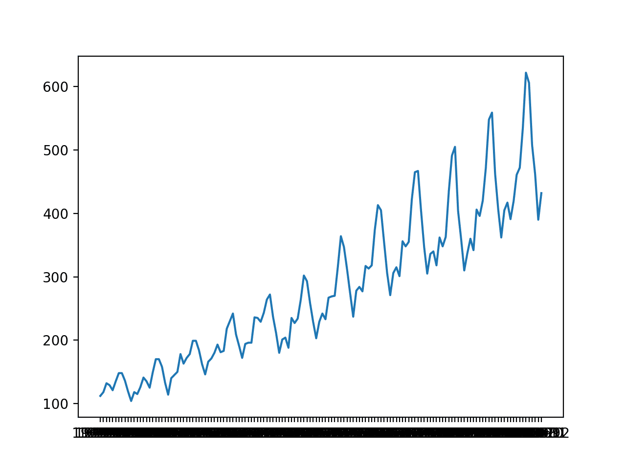
The ‘monthly airline passenger‘ dataset summarizes the monthly total number of international passengers in thousands on for an airline from 1949 to 1960.
Running the example first prints the shape of the dataset.
1
(144, 1)
The dataset is monthly and has 12 years, or 144 observations. In our testing, we will use the last year, or 12 observations, as the test set.
A line plot is created. The dataset has an obvious trend and seasonal component. The period of the seasonal component is 12 months.
Line Plot of Monthly International Airline Passengers
In this tutorial, we will introduce the tools for grid searching, but we will not optimize the model hyperparameters for this problem. Instead, we will demonstrate how to grid search the deep learning model hyperparameters generally and find models with some skill compared to a naive model.
From prior experiments, a naive model can achieve a root mean squared error, or RMSE, of 50.70 (remember the units are thousands of passengers) by persisting the value from 12 months ago (relative index -12).
The performance of this naive model provides a bound on a model that is considered skillful for this problem. Any model that achieves a predictive performance of lower than 50.70 on the last 12 months has skill.
It should be noted that a tuned ETS model can achieve an RMSE of 17.09 and a tuned SARIMA can achieve an RMSE of 13.89. These provide a lower bound on the expectations of a well-tuned deep learning model for this problem.
Now that we have defined our problem and expectations of model skill, we can look at defining the grid search test harness.
Grid Search Framework
In this section, we will develop a grid search test harness that can be used to evaluate a range of hyperparameters for different neural network models, such as MLPs, CNNs, and LSTMs.
This section is divided into the following parts:
Train-Test Split
Series as Supervised Learning
Walk-Forward Validation
Repeat Evaluation
Summarize Performance
Worked Example
Train-Test Split
The first step is to split the loaded series into train and test sets.
We will use the first 11 years (132 observations) for training and the last 12 for the test set.
The train_test_split() function below will split the series taking the raw observations and the number of observations to use in the test set as arguments.
1
2
3
# split a univariate dataset into train/test sets
def train_test_split(data,n_test):
returndata[:-n_test],data[-n_test:]
Series as Supervised Learning
Next, we need to be able to frame the univariate series of observations as a supervised learning problem so that we can train neural network models.
A supervised learning framing of a series means that the data needs to be split into multiple examples that the model learns from and generalizes across.
Each sample must have both an input component and an output component.
The input component will be some number of prior observations, such as three years, or 36 time steps.
The output component will be the total sales in the next month because we are interested in developing a model to make one-step forecasts.
We can implement this using the shift() function on the pandas DataFrame. It allows us to shift a column down (forward in time) or back (backward in time). We can take the series as a column of data, then create multiple copies of the column, shifted forward or backward in time in order to create the samples with the input and output elements we require.
When a series is shifted down, NaN values are introduced because we don’t have values beyond the start of the series.
For example, the series defined as a column:
1
2
3
4
5
(t)
1
2
3
4
This column can be shifted and inserted as a column beforehand:
1
2
3
4
5
6
(t-1), (t)
Nan, 1
1, 2
2, 3
3, 4
4 NaN
We can see that on the second row, the value 1 is provided as input as an observation at the prior time step, and 2 is the next value in the series that can be predicted, or learned by the model to be predicted when 1 is presented as input.
Rows with NaN values can be removed.
The series_to_supervised() function below implements this behavior, allowing you to specify the number of lag observations to use in the input and the number to use in the output for each sample. It will also remove rows that have NaN values as they cannot be used to train or test a model.
1
2
3
4
5
6
7
8
9
10
11
12
13
14
15
# transform list into supervised learning format
def series_to_supervised(data,n_in=1,n_out=1):
df=DataFrame(data)
cols=list()
# input sequence (t-n, ... t-1)
foriinrange(n_in,0,-1):
cols.append(df.shift(i))
# forecast sequence (t, t+1, ... t+n)
foriinrange(0,n_out):
cols.append(df.shift(-i))
# put it all together
agg=concat(cols,axis=1)
# drop rows with NaN values
agg.dropna(inplace=True)
returnagg.values
Walk-Forward Validation
Time series forecasting models can be evaluated on a test set using walk-forward validation.
Walk-forward validation is an approach where the model makes a forecast for each observation in the test dataset one at a time. After each forecast is made for a time step in the test dataset, the true observation for the forecast is added to the test dataset and made available to the model.
Simpler models can be refit with the observation prior to making the subsequent prediction. More complex models, such as neural networks, are not refit given the much greater computational cost.
Nevertheless, the true observation for the time step can then be used as part of the input for making the prediction on the next time step.
First, the dataset is split into train and test sets. We will call the train_test_split() function to perform this split and pass in the pre-specified number of observations to use as the test data.
A model will be fit once on the training dataset for a given configuration.
We will define a generic model_fit() function to perform this operation that can be filled in for the given type of neural network that we may be interested in later. The function takes the training dataset and the model configuration and returns the fit model ready for making predictions.
1
2
3
# fit a model
def model_fit(train,config):
returnNone
Each time step of the test dataset is enumerated. A prediction is made using the fit model.
Again, we will define a generic function named model_predict() that takes the fit model, the history, and the model configuration and makes a single one-step prediction.
1
2
3
# forecast with a pre-fit model
def model_predict(model,history,config):
return0.0
The prediction is added to a list of predictions and the true observation from the test set is added to a list of observations that was seeded with all observations from the training dataset. This list is built up during each step in the walk-forward validation, allowing the model to make a one-step prediction using the most recent history.
All of the predictions can then be compared to the true values in the test set and an error measure calculated.
We will calculate the root mean squared error, or RMSE, between predictions and the true values.
RMSE is calculated as the square root of the average of the squared differences between the forecasts and the actual values. The measure_rmse() implements this below using the mean_squared_error() scikit-learn function to first calculate the mean squared error, or MSE, before calculating the square root.
1
2
3
# root mean squared error or rmse
def measure_rmse(actual,predicted):
returnsqrt(mean_squared_error(actual,predicted))
The complete walk_forward_validation() function that ties all of this together is listed below.
It takes the dataset, the number of observations to use as the test set, and the configuration for the model, and returns the RMSE for the model performance on the test set.
1
2
3
4
5
6
7
8
9
10
11
12
13
14
15
16
17
18
19
20
21
# walk-forward validation for univariate data
def walk_forward_validation(data,n_test,cfg):
predictions=list()
# split dataset
train,test=train_test_split(data,n_test)
# fit model
model=model_fit(train,cfg)
# seed history with training dataset
history=[xforxintrain]
# step over each time-step in the test set
foriinrange(len(test)):
# fit model and make forecast for history
yhat=model_predict(model,history,cfg)
# store forecast in list of predictions
predictions.append(yhat)
# add actual observation to history for the next loop
history.append(test[i])
# estimate prediction error
error=measure_rmse(test,predictions)
print(' > %.3f'%error)
returnerror
Repeat Evaluation
Neural network models are stochastic.
This means that, given the same model configuration and the same training dataset, a different internal set of weights will result each time the model is trained that will, in turn, have a different performance.
This is a benefit, allowing the model to be adaptive and find high performing configurations to complex problems.
It is also a problem when evaluating the performance of a model and in choosing a final model to use to make predictions.
To address model evaluation, we will evaluate a model configuration multiple times via walk-forward validation and report the error as the average error across each evaluation.
This is not always possible for large neural networks and may only make sense for small networks that can be fit in minutes or hours.
The repeat_evaluate() function below implements this and allows the number of repeats to be specified as an optional parameter that defaults to 10 and returns the mean RMSE score from all repeats.
All that is left is a function to drive the search. We can define a grid_search() function that takes the dataset, a list of configurations to search, and the number of observations to use as the test set and perform the search.
Once mean scores are calculated for each config, the list of configurations is sorted in ascending order so that the best scores are listed first.
Now that we have defined the elements of the test harness, we can tie them all together and define a simple persistence model.
We do not need to fit a model so the model_fit() function will be implemented to simply return None.
1
2
3
# fit a model
def model_fit(train,config):
returnNone
We will use the config to define a list of index offsets in the prior observations relative to the time to be forecasted that will be used as the prediction. For example, 12 will use the observation 12 months ago (-12) relative to the time to be forecasted.
1
2
# define config
cfg_list=[1,6,12,24,36]
The model_predict() function can be implemented to use this configuration to persist the value at the negative relative offset.
1
2
3
# forecast with a pre-fit model
def model_predict(model,history,offset):
history[-offset]
The complete example of using the framework with a simple persistence model is listed below.
1
2
3
4
5
6
7
8
9
10
11
12
13
14
15
16
17
18
19
20
21
22
23
24
25
26
27
28
29
30
31
32
33
34
35
36
37
38
39
40
41
42
43
44
45
46
47
48
49
50
51
52
53
54
55
56
57
58
59
60
61
62
63
64
65
66
67
68
69
70
71
72
73
74
75
76
# grid search persistence models for airline passengers
from math import sqrt
from numpy import mean
from pandas import read_csv
from sklearn.metrics import mean_squared_error
# split a univariate dataset into train/test sets
def train_test_split(data,n_test):
returndata[:-n_test],data[-n_test:]
# root mean squared error or rmse
def measure_rmse(actual,predicted):
returnsqrt(mean_squared_error(actual,predicted))
# fit a model
def model_fit(train,config):
returnNone
# forecast with a pre-fit model
def model_predict(model,history,offset):
returnhistory[-offset]
# walk-forward validation for univariate data
def walk_forward_validation(data,n_test,cfg):
predictions=list()
# split dataset
train,test=train_test_split(data,n_test)
# fit model
model=model_fit(train,cfg)
# seed history with training dataset
history=[xforxintrain]
# step over each time-step in the test set
foriinrange(len(test)):
# fit model and make forecast for history
yhat=model_predict(model,history,cfg)
# store forecast in list of predictions
predictions.append(yhat)
# add actual observation to history for the next loop
Running the example prints the RMSE of the model evaluated using walk-forward validation on the final 12 months of data.
Each model configuration is evaluated 10 times, although, because the model has no stochastic element, the score is the same each time.
At the end of the run, the configurations and RMSE for the top three performing model configurations are reported.
We can see, as we might have expected, that persisting the value from one year ago (relative offset -12) resulted in the best performance for the persistence model.
1
2
3
4
5
6
7
8
9
10
11
...
> 110.274
> 110.274
> 110.274
> Model[36] 110.274
done
12 50.708316214732804
1 53.1515129919491
24 97.10990337413241
36 110.27352356753639
6 126.73495965991387
Now that we have a robust test harness for grid searching model hyperparameters, we can use it to evaluate a suite of neural network models.
Need help with Deep Learning for Time Series?
Take my free 7-day email crash course now (with sample code).
Click to sign-up and also get a free PDF Ebook version of the course.
Grid Search Multilayer Perceptron
There are many aspects of the MLP that we may wish to tune.
We will define a very simple model with one hidden layer and define five hyperparameters to tune. They are:
n_input: The number of prior inputs to use as input for the model (e.g. 12 months).
n_nodes: The number of nodes to use in the hidden layer (e.g. 50).
n_epochs: The number of training epochs (e.g. 1000).
n_batch: The number of samples to include in each mini-batch (e.g. 32).
n_diff: The difference order (e.g. 0 or 12).
Modern neural networks can handle raw data with little pre-processing, such as scaling and differencing. Nevertheless, when it comes to time series data, sometimes differencing the series can make a problem easier to model.
Recall that differencing is the transform of the data such that a value of a prior observation is subtracted from the current observation, removing trend or seasonality structure.
We will add support for differencing to the grid search test harness, just in case it adds value to your specific problem. It does add value for the internal airline passengers dataset.
The difference() function below will calculate the difference of a given order for the dataset.
Differencing will be optional, where an order of 0 suggests no differencing, whereas an order 1 or order 12 will require that the data be differenced prior to fitting the model and that the predictions of the model will need the differencing reversed prior to returning the forecast.
We can now define the elements required to fit the MLP model in the test harness.
First, we must unpack the list of hyperparameters.
1
2
# unpack config
n_input,n_nodes,n_epochs,n_batch,n_diff=config
Next, we must prepare the data, including the differencing, transforming the data to a supervised format and separating out the input and output aspects of the data samples.
1
2
3
4
5
6
7
# prepare data
ifn_diff>0:
train=difference(train,n_diff)
# transform series into supervised format
data=series_to_supervised(train,n_in=n_input)
# separate inputs and outputs
train_x,train_y=data[:,:-1],data[:,-1]
We can now define and fit the model with the provided configuration.
The five chosen hyperparameters are by no means the only or best hyperparameters of the model to tune. You may modify the function to tune other parameters, such as the addition and size of more hidden layers and much more.
Once the model is fit, we can use it to make forecasts.
If the data was differenced, the difference must be inverted for the prediction of the model. This involves adding the value at the relative offset from the history back to the value predicted by the model.
1
2
3
4
5
6
7
# invert difference
correction=0.0
ifn_diff>0:
correction=history[-n_diff]
...
# correct forecast if it was differenced
returncorrection+yhat[0]
It also means that the history must be differenced so that the input data used to make the prediction has the expected form.
1
2
# calculate difference
history=difference(history,n_diff)
Once prepared, we can use the history data to create a single sample as input to the model for making a one-step prediction.
The shape of one sample must be [1, n_input] where n_input is the chosen number of lag observations to use.
The complete implementation of the model_predict() function is listed below.
Next, we must define the range of values to try for each hyperparameter.
We can define a model_configs() function that creates a list of the different combinations of parameters to try.
We will define a small subset of configurations to try as an example, including a differencing of 12 months, which we expect will be required. You are encouraged to experiment with standalone models, review learning curve diagnostic plots, and use information about the domain to set ranges of values of the hyperparameters to grid search.
You are also encouraged to repeat the grid search to narrow in on ranges of values that appear to show better performance.
An implementation of the model_configs() function is listed below.
1
2
3
4
5
6
7
8
9
10
11
12
13
14
15
16
17
18
19
# create a list of configs to try
def model_configs():
# define scope of configs
n_input=[12]
n_nodes=[50,100]
n_epochs=[100]
n_batch=[1,150]
n_diff=[0,12]
# create configs
configs=list()
foriinn_input:
forjinn_nodes:
forkinn_epochs:
forlinn_batch:
forminn_diff:
cfg=[i,j,k,l,m]
configs.append(cfg)
print('Total configs: %d'%len(configs))
returnconfigs
We now have all of the pieces needed to grid search MLP models for a univariate time series forecasting problem.
Running the example, we can see that there are a total of eight configurations to be evaluated by the framework.
Note: Your results may vary given the stochastic nature of the algorithm or evaluation procedure, or differences in numerical precision. Consider running the example a few times and compare the average outcome.
Each config will be evaluated 10 times; that means 10 models will be created and evaluated using walk-forward validation to calculate an RMSE score before an average of those 10 scores is reported and used to score the configuration.
The scores are then sorted and the top 3 configurations with the lowest RMSE are reported at the end. A skillful model configuration was found as compared to a naive model that reported an RMSE of 50.70.
We can see that the best RMSE of 18.98 was achieved with a configuration of [12, 100, 100, 1, 12], which we know can be interpreted as:
n_input: 12
n_nodes: 100
n_epochs: 100
n_batch: 1
n_diff: 12
A truncated example output of the grid search is listed below.
1
2
3
4
5
6
7
8
9
10
11
12
13
14
15
Total configs: 8
> 20.707
> 29.111
> 17.499
> 18.918
> 28.817
...
> 21.015
> 20.208
> 18.503
> Model[[12, 100, 100, 150, 12]] 19.674
done
[12, 100, 100, 1, 12] 18.982720013625606
[12, 50, 100, 150, 12] 19.33004059448595
[12, 100, 100, 1, 0] 19.5389405532858
Grid Search Convolutional Neural Network
We can now adapt the framework to grid search CNN models.
Much the same set of hyperparameters can be searched as with the MLP model, except the number of nodes in the hidden layer can be replaced by the number of filter maps and kernel size in the convolutional layers.
The chosen set of hyperparameters to grid search in the CNN model are as follows:
n_input: The number of prior inputs to use as input for the model (e.g. 12 months).
n_filters: The number of filter maps in the convolutional layer (e.g. 32).
n_kernel: The kernel size in the convolutional layer (e.g. 3).
n_epochs: The number of training epochs (e.g. 1000).
n_batch: The number of samples to include in each mini-batch (e.g. 32).
n_diff: The difference order (e.g. 0 or 12).
Some additional hyperparameters that you may wish to investigate are the use of two convolutional layers before a pooling layer, the repetition of the convolutional and pooling layer pattern, the use of dropout, and more.
We will define a very simple CNN model with one convolutional layer and one max pooling layer.
The data must be prepared in much the same way as for the MLP.
Unlike the MLP that expects the input data to have the shape [samples, features], the 1D CNN model expects the data to have the shape [samples, timesteps, features] where features maps onto channels and in this case 1 for the one variable we measure each month.
1
2
3
# reshape input data into [samples, timesteps, features]
Finally, we can define a list of configurations for the model to evaluate. As before, we can do this by defining lists of hyperparameter values to try that are combined into a list. We will try a small number of configurations to ensure the example executes in a reasonable amount of time.
The complete model_configs() function is listed below.
1
2
3
4
5
6
7
8
9
10
11
12
13
14
15
16
17
18
19
20
21
# create a list of configs to try
def model_configs():
# define scope of configs
n_input=[12]
n_filters=[64]
n_kernels=[3,5]
n_epochs=[100]
n_batch=[1,150]
n_diff=[0,12]
# create configs
configs=list()
forainn_input:
forbinn_filters:
forcinn_kernels:
fordinn_epochs:
foreinn_batch:
forfinn_diff:
cfg=[a,b,c,d,e,f]
configs.append(cfg)
print('Total configs: %d'%len(configs))
returnconfigs
We now have all of the elements needed to grid search the hyperparameters of a convolutional neural network for univariate time series forecasting.
The complete example is listed below.
1
2
3
4
5
6
7
8
9
10
11
12
13
14
15
16
17
18
19
20
21
22
23
24
25
26
27
28
29
30
31
32
33
34
35
36
37
38
39
40
41
42
43
44
45
46
47
48
49
50
51
52
53
54
55
56
57
58
59
60
61
62
63
64
65
66
67
68
69
70
71
72
73
74
75
76
77
78
79
80
81
82
83
84
85
86
87
88
89
90
91
92
93
94
95
96
97
98
99
100
101
102
103
104
105
106
107
108
109
110
111
112
113
114
115
116
117
118
119
120
121
122
123
124
125
126
127
128
129
130
131
132
133
134
135
136
137
138
139
140
141
142
143
144
145
146
147
148
149
150
151
152
153
154
155
156
157
# grid search cnn for airline passengers
from math import sqrt
from numpy import array
from numpy import mean
from pandas import DataFrame
from pandas import concat
from pandas import read_csv
from sklearn.metrics import mean_squared_error
from keras.models import Sequential
from keras.layers import Dense
from keras.layers import Flatten
from keras.layers.convolutional import Conv1D
from keras.layers.convolutional import MaxPooling1D
Running the example, we can see that only eight distinct configurations are evaluated.
Note: Your results may vary given the stochastic nature of the algorithm or evaluation procedure, or differences in numerical precision. Consider running the example a few times and compare the average outcome.
We can see that a configuration of [12, 64, 5, 100, 1, 12] achieved an RMSE of 18.89, which is skillful as compared to a naive forecast model that achieved 50.70.
We can unpack this configuration as:
n_input: 12
n_filters: 64
n_kernel: 5
n_epochs: 100
n_batch: 1
n_diff: 12
A truncated example output of the grid search is listed below.
1
2
3
4
5
6
7
8
9
10
11
12
13
Total configs: 8
> 23.372
> 28.317
> 31.070
...
> 20.923
> 18.700
> 18.210
> Model[[12, 64, 5, 100, 150, 12]] 19.152
done
[12, 64, 5, 100, 1, 12] 18.89593462072732
[12, 64, 5, 100, 150, 12] 19.152486150334234
[12, 64, 3, 100, 150, 12] 19.44680151564605
Grid Search Long Short-Term Memory Network
We can now adopt the framework for grid searching the hyperparameters of an LSTM model.
The hyperparameters for the LSTM model will be the same five as the MLP; they are:
n_input: The number of prior inputs to use as input for the model (e.g. 12 months).
n_nodes: The number of nodes to use in the hidden layer (e.g. 50).
n_epochs: The number of training epochs (e.g. 1000).
n_batch: The number of samples to include in each mini-batch (e.g. 32).
n_diff: The difference order (e.g. 0 or 12).
We will define a simple LSTM model with a single hidden LSTM layer and the number of nodes specifying the number of units in this layer.
It may be interesting to explore tuning additional configurations such as the use of a bidirectional input layer, stacked LSTM layers, and even hybrid models with CNN or ConvLSTM input models.
As with the CNN model, the LSTM model expects input data to have a three-dimensional shape for the samples, time steps, and features.
1
2
3
# reshape input data into [samples, timesteps, features]
Running the example, we can see that only two distinct configurations are evaluated.
Note: Your results may vary given the stochastic nature of the algorithm or evaluation procedure, or differences in numerical precision. Consider running the example a few times and compare the average outcome.
We can see that a configuration of [12, 100, 50, 1, 12] achieved an RMSE of 21.24, which is skillful as compared to a naive forecast model that achieved 50.70.
The model requires a lot more tuning and may do much better with a hybrid configuration, such as having a CNN model as input.
We can unpack this configuration as:
n_input: 12
n_nodes: 100
n_epochs: 50
n_batch: 1
n_diff: 12
A truncated example output of the grid search is listed below.
1
2
3
4
5
6
7
8
9
10
11
12
Total configs: 2
> 20.488
> 17.718
> 21.213
...
> 22.300
> 20.311
> 21.322
> Model[[12, 100, 50, 150, 12]] 21.260
done
[12, 100, 50, 1, 12] 21.243775750634093
[12, 100, 50, 150, 12] 21.259553398553606
Extensions
This section lists some ideas for extending the tutorial that you may wish to explore.
More Configurations. Explore a large suite of configurations for one of the models and see if you can find a configuration that results in better performance.
Data Scaling. Update the grid search framework to also support the scaling (normalization and/or standardization) of data both before fitting the model and inverting the transform for predictions.
Network Architecture. Explore the grid searching larger architectural changes for a given model, such as the addition of more hidden layers.
New Dataset. Explore the grid search of a given model in a new univariate time series dataset.
Multivariate. Update the grid search framework to support small multivariate time series datasets, e.g. datasets with multiple input variables.
If you explore any of these extensions, I’d love to know.
Further Reading
This section provides more resources on the topic if you are looking to go deeper.
in section “Grid Search Long Short-Term Memory Network”, why do you only use training data to make “series_to_supervised” instead of the whole original one. Thanks!
A very complete and rich hyperparameters tutorial (i.e. a sensitivity analysis of model errors output vs hyperparameters inputs). Even very useful in order to practice model definitions as MLP, CNN and LSTM. In addition to practice with modules or function to standardize the code.Thank you very much. I got same results as you but with some first decimal changes !.
My comments, if useful , are related to two main cores regarding machine learning structure:
– The first one is, related to dataset FRAMING (i.e. prepare inputs vs labels (outputs) and train vs test split from dataset). the function “def train_test_split” is very clear , but the function “def series_to_supervised” is less clear. Probably because the use of methodS for dataframe .shift[i] for backward input is counterintuitive with shift[-i] for forward or labels :-). My suggestion is to use some plot or drawings to show more clearly how those inputs-labels are caught from original dataset cols.
-The second one is related to how DIMENSION and RESHAPING matching. So the argument of first layer (input_shape=) of model definition for different ones (MLP,CNN,LSTM), or how to reshape training_data (input data into [samples, timesteps, features] into different model_fit function, or finally x_input into different model_predict function (x_input = array(history[-n_input:]).reshape((1, n_input, 1)). One more time my suggestion is to use some plot or drawings or matrices to see how those dimension must match the different input parts of the process (layers, training, predicting,..).
From my experience those use to be the hard part of the code …I always have to work hard on how to handle them. So emphasizing those hard cores issues during code presentation… could help a lot .
1) I see your useful function valid for single-steps or multi-steps and univariate or multivariate TIMESERIES:
“def series_to_supervised(data, n_in=1, n_out=1, dropnan=True)”:
But also I see also the guy who set up this “shift” function in pandas decided to put shift(+i) to go backward (t-1) and shift (-1) to go forward t+1 :a little counterintuitive :–)
thks.
2) I see now more clearly the meaning of 3D dimensions for LSTM input ( I guess is the same for CNN), as [samples, timesteps, features)…thanks
But also I see how when you define the data 3D shape in [samples, timesteps, features] later when you use the input_shape argument of LST it must be omitted the samples dimension, and only retain in the set up a 2D tuple [timesteps, features] and also in the x_input for model_predict to set up samples for 1 for sample [1, timesteps=1, features)=1
I hope more examples give us more easy understanding
Great tutorial ! Please let me know how to predict for future data for 1 value for LSTM.
For, example, i have a trained LSTM and want to predict for t(n+1).
The example above only show prediction using the test set.
LSTMs may have a place on multivariate and multistep problems, but my testing shows CNNs and friends (convlstm and cnnlstm) still outperform vanilla lstm.
Hello Jason,
Thank you for this post.
I am currently exploring multivariate multi step grid search. I am using walk-forward method and I have a question, can I use the walk-forward method to multi step problem?
the folds in walk-forward problem will be (Correct me if I am wrong) :
input [1, 2, 3 ] output [4,5]
input [2, 3, 4 ] output [5,6]
input [3, 4, 5 ] output [6,7]
and for multi variate multi step I will have:
input [[1,2,3 ] [11, 22 , 33 ] [111,222,333] ] output [4,5, 44, 55 , 444,555]
input [[2,3,4 ] [22 , 33, 44 ] [222,333,444] ] output [5,6, 55 ,66,555,666]
since the output will be flattened.
We use Validation sets to tune a model and Test Set Evaluation Model.
Time series forecasting models can be evaluated on a test set using walk-forward validation.Are we missing validation sets?In fact, we use test sets to tune a model.
You could split train into train and val sets, find a model via walk-forward on the train set, tune it via walk-forward on the val set, then evaluate it via walk-forward on the test set.
Thanks!I think of another problem.
We divide data sets in chronological order, so we separate validation set and test set. Our model can not learn the information of validation set. It is likely that the data of validation set must be learned. Perhaps the verification set is not important for time series. However, the loss of new time information may lead to worse model performance.
The test harness and approach to evaluating models is often specific for a given project. You must design it so that you are comfortable and confident with the estimated performance of the models.
Hello. Congratulations on the content. Could it be possible to implement parallelism in this code? How could I force the use of all available CPU cores?
Jason, thank you so much for sharing your knowledge with us. Thank you very much.
I would like to ask if this base (monthly-airline-passengers.csv) had 2,000 rows and two columns as inputs, eg ticket value and fuel value, output would be passenger numbers, it would be possible to apply this code LSTM?
Wondering if you have attempted to set the numpy and Tensorflow random number seeds to reproduce results with this example. I have read your post on Keras reproducibility and have tried to implement the suggestions but to no avail. Do you think the example model above is too complicated to reproduce results?
Why don’t you use a GridSearchCV vs. writing your own function? I have read your code and it seems to me that your code structured the same way as pre-built GridSearchCV (bunch of for loops). Is there a reason you didn’t want to use GridSearchCV/RandomizedSearchCV?
I see. Do you have an example how to use GridSearchCV (from scikit learn) with LSTM? I keep having problems with shapes (GridSearch needs input array to have shape of [n_samples, n_features], while LSTM asks for [samples, timesteps, features])?
Excellent post! Extremely valuable! Two questions.
1) What does “history” do in walk forward validation?
2) In the same code following “history”, as far as I see, you predict one example at a time for each test set. Can we (or should we) do 100 at a time like a batch to make this faster?
Thanks
Hi Jason,
I have learned a lot about LSTM’s reading your excellent articles.
In this code I believe you miss the last entry of your test_x array, because you do not add any value from test_x in the first loop.
for i in range(len(test)):
# fit model and make forecast for history
yhat = model_predict(model, history, cfg)
# store forecast in list of predictions
predictions.append(yhat)
# add actual observation to history for the next loop
history.append(test[i])
Moving “history.append(test[i])” to the top of the loop prior to calling model_predict will start adding test_x values and also consider the last entry of test_x.
What do you think?
Hi Jason. I follow your guides quite a bit, and i have a question regarding your answer here. As far as i’ve understood, the GridsearchCV is unusable for timeseries data due to the crossvalidation removing the dependency of the order of samples. But what if i use the KerasRegressor (like you use the KerasClassifier in another of your great posts) as a wrapper for the GridsearchCV function, and then ‘hack’ the function to not use crossvalidation like this post suggests: https://stackoverflow.com/questions/44636370/scikit-learn-gridsearchcv-without-cross-validation-unsupervised-learning
One would simply set the cv parameter like such: cv=ShuffleSplit(test_size=0.20, n_splits=1)
That sounds possible, but I would prefer to write my own version of GridSearchCV for time series data instead, so the intention is clearer. The way of doing cross validation in time series is a bit different. Hence I am not surprised to see you try this.
Does the line with “scores = scores =” have any significance? I see this format throughout your post, but am unsure if the assignment is duplicated, or if I am missing something.
Hello. Thanks for the awesome tutorial. However, I am confused about the history. For the MLP code, it seems that the only the last n_input samples in the history are used for the prediction within the walk forward validation.
In the first loop iteration the last n_input samples of the training data are used. Then for every other iteration, the first n_input testing samples are used.
If this is the case, why does the history have to be initialized to the entire training set? Also, why don’t we just use the testing data to calculate the error and just not use history at all?
Hello, thanks for your posts, I would like to ask, I’m going to make an lstm neural network for predicting time series. And such a question, can I train one model and use it in all forecasts? Is there a problem that the input data may differ each time (the amount of input data), or do I need to train a new model each time for new data?
3. Also which of the following approaches is better:
– Tree Parzen Estimator (TPE)
– Bayesian Optimization (Gaussian Process surrogate)
– Sequential Model-based Algorithm Configuration (SMAC)
– Random forest regression
This is an excelent exercise. I want to know if you have the code of MLP for Multivariables. Please, I need this urgent with differents windows for each variable. Thank you very much. You have help me a lot of.
Thanks for the post. I m interested to implement as Deep-Q learning time-series grid search I m taking Environment( framework) as tuning different parameters, state as observations and test set to search. the best action path will be the best of scores?.is it possible to implement it? can you please give me any ideas to implement as Deep Q learning time series
thanks for your response! What you are doing here is that for one configuration, you are repeating your evaluation 10 times and calculating the mean of the scores for this configuration. Also, in each evaluation for one configuration, you predict for one time step by looking for past 12 months and then include that time step to predict for the next and so on(using history).
Also, in my case my data is already windowed with past 5 days windows using which I need to predict the current day’s trading signal – up/down , so that way i do not require history.
Finally, my question is if I need to tune hyperparameters on this windowed data, then I do not require history but then how should I do the splits ? Can I predict for multiple windows in the test set at once and then do the rolling or expanding analysis? for example I have 4 years data, so train the model for 1.5years and predict for 6 months and then include this 6 months of the data for training and text for next 6months and so on like expanding analysis. Like that there will be 5-6 models for one configuration and I will obtain the scores from all the models and average them out.
Yes, I skipped re-training for performance reasons – it’s slow. You can retrain if you like.
Test each set of hyperparameters in the same way as in the tutorial above – e.g. walk forward validation on a test subset of the data. The size of the test set is up to you, ensure it is representative of the way you intend to use the final model.
Thanks for this tutorial, I love the way you set out your solutions.
I have a few questions regarding the LSTM section:
1.) How come we difference the data after splitting into to train/ test? Wouldn’t it make more sense to do this before?
2.) Altering the difference and input paramaters affect the length of the validation data set. Wouldn’t you expect this to have a confounding effect on the RMSE score?
Hi Jason,
Excellent post. I have also purchased your book on Time Series Forecasting. I am looking for some advice on time series clustering and forecasting. The company I am working with has 150k customer and they supply electricity. They would like to build model for each customer to predict their consumption requirement. I have been working with the data for few months and the consumption data are very much alike for eache customer. I tried to cluster them but b=very very difficult to create multiple cluster. Also it is not practical to build 150k models. Do you have general advice or a post will be nice on time series forecasting for more than 1 product/customer.
Thanks for responding me. It is indeed an interesting project but very challenging. I am commenting on your suggestions
Develop one model per site. (150k models seems impossible)
Develop one model per group of sites. ( I tried to group them by using scipy.cluster.hierarchy and all of them seems to formed into one group. so not very helpful)
Develop one model for all sites. (Yes this seems okay but again each customer is different and their usage pattern is also different and the company is not interested in this one 🙁 )
Hybrid of the above.
Ensemble of the above.
Do you have any other suggestion? or any book or reference to look for?
For example, if I do:
model = Sequential()
model.add(LSTM(n_nodes, activation=’relu’, input_dim=n_input))
model.add(Dense(1), activation=’linear’)
model.compile(loss=’mse’, optimizer=’adam’)
Is it correct to say that for output I will use activation linear, but for the LSTM I will use ‘relu’ (replacing the already internal sigmoid and tahn)?
Very nice tutorial. I’m interested in exploring more in terms of the network architecture. But I found that tuning LSTM layers is different from the other hyperparameters in this tutorial because it’s not just simply tuning a value but need to declare each layer, if I’m not mistaken.
I’d really appreciate it if you could share a tutorial or reference on tuning the hidden layer.
I am working on a Time Series problem. I have the historical data of the 5 last years but the data from April 2020 to June 2020 are missing as the business close during the COVID-19 lockdown. So here, I have the daily data missing for 3 months. Are the traditional imputation strategies (KNN for example) can work for such a long timeframe? What is your suggestion?
Amazing tutorial, thank you! I am struggling with a multivariate LSTM grid search for quite some time now, as I am quite new to the programming side. It is hard to find multivariate examples online. Any suggestion how to transform your example to multivariate with lots of features?
Appreciate your help and your tutorial, it is amazing!
Hi Jason, thanks for your excellent tutorials.
I have a question reguarding Grid Search for multi-step predictions (step=3) in univariate time series.
When I use your Grid Search for my problem, I get this error in walk_forward_validation(data, n_test, cfg):
“y_true and y_pred have different number of output (1!=3)”.
def walk_forward_validation(data, n_test, cfg):
predictions = list()
# split dataset
train, test = train_test_split(data, n_test)
# fit model
model = model_fit(train, cfg)
# seed history with training dataset
history = [x for x in train]
# step over each time-step in the test set
for i in range(len(test)):
# fit model and make forecast for history
yhat = model_predict(model, history, cfg)
# store forecast in list of predictions
predictions.append(yhat)
# add actual observation to history for the next loop
history.append(test[i])
# estimate prediction error
error = measure_rmse(test, predictions)
print(‘ > %.3f’ % error)
return error
Sorry to hear that, it suggests your predictions and test data do not match in terms of the number of observations, you need to change/debug your code.
Great post! How would you approach the problem of sales forecasting for multiple stores? Would you do the hyper-param tuning per store and loop over all stores (so you’ll have 1 set of param for each store)? Or would you combine all stores into 1 dataframe with store ID and tune in 1 go?
Hi, great tutorial!
Is there a way to save the best model weights after the grid search is complete? If I use ModelCheckpoint as a callback this just save the best performing model in the last grid search iteration, which is not guaranteed to be the best overall.
I am asking this because for some reason even if I set the random seed and I save the value of the best-performing parameters I get different predictions when I re-fit it on the same data
It is the best to re-train the model after grid search as grid search is to help you evaluate the model design rather than create a model for permanent use. But if you insist, you need to modify walk_forward_validation() function as it is where the model is created but discarded after the function return.
Hi! Thank you so much for your work and tutorials!
I’m currently working on a model with 50 samples. And I’m not if I’m understanding well the concept of walk-forward validation. Do I need to make a train-validation-test separation, and then apply walk forward validation on the train-validation data to get the hyper parameters. And then applying walk forward testing for the train-test data.
Because from what I understand, by using walk forward validation you are both tuning the hyperparameters models and testing the model, so we only need a train-test separation?
Which option is the best?
An awesome and inspiring article…as most of your articles in your web.
Well the question is that in case the model will not get refit inside the walk_forward_validation() for loop, I think this procedure can be simplified, let’s me explain with a contrived example:
I’m eager to help, but I just don’t have the capacity to debug code for you.
I am happy to make some suggestions:
Consider aggressively cutting the code back to the minimum required. This will help you isolate the problem and focus on it.
Consider cutting the problem back to just one or a few simple examples.
Consider finding other similar code examples that do work and slowly modify them to meet your needs. This might expose your misstep.
Consider posting your question and code to StackOverflow.
Thanks for the tutorial.
In walk forward validation function definition, should you not call the model_fit() function inside the for loop instead of outside for loop.
# fit model
model = model_fit(train, cfg)
for i in range(len(test)):
This model_fit() should be inside for loop as forecasts are appended in history which will serve as train in model_fit() function. Calling it outside defeats the whole purpose of walk forward validation concept.
————————————————————————————————————————————–
In this tutorial https://machinelearningmastery.com/random-forest-for-time-series-forecasting,
random_forest_forecast() function is called inside the for loop which fits the model and makes a prediction.
# code from this tutorial just above
def walk_forward_validation(data, n_test):
for i in range(len(test)):
yhat = random_forest_forecast(history, testX)
Please correct me if I am wrong in my understanding or pointing this out.


Thank you for providing such wonderful information.
I’m glad it helped.
in section “Grid Search Long Short-Term Memory Network”, why do you only use training data to make “series_to_supervised” instead of the whole original one. Thanks!
Because we should hold out a test set to evaluate our model is a good one.
Just wanted to say thank you for your most excellent tutorials. They have helped me tremendously.
Thanks, I’m happy to hear that.
Hola Jason:
A very complete and rich hyperparameters tutorial (i.e. a sensitivity analysis of model errors output vs hyperparameters inputs). Even very useful in order to practice model definitions as MLP, CNN and LSTM. In addition to practice with modules or function to standardize the code.Thank you very much. I got same results as you but with some first decimal changes !.
My comments, if useful , are related to two main cores regarding machine learning structure:
– The first one is, related to dataset FRAMING (i.e. prepare inputs vs labels (outputs) and train vs test split from dataset). the function “def train_test_split” is very clear , but the function “def series_to_supervised” is less clear. Probably because the use of methodS for dataframe .shift[i] for backward input is counterintuitive with shift[-i] for forward or labels :-). My suggestion is to use some plot or drawings to show more clearly how those inputs-labels are caught from original dataset cols.
-The second one is related to how DIMENSION and RESHAPING matching. So the argument of first layer (input_shape=) of model definition for different ones (MLP,CNN,LSTM), or how to reshape training_data (input data into [samples, timesteps, features] into different model_fit function, or finally x_input into different model_predict function (x_input = array(history[-n_input:]).reshape((1, n_input, 1)). One more time my suggestion is to use some plot or drawings or matrices to see how those dimension must match the different input parts of the process (layers, training, predicting,..).
From my experience those use to be the hard part of the code …I always have to work hard on how to handle them. So emphasizing those hard cores issues during code presentation… could help a lot .
thank you for your job.
Thanks.
This post may help in understanding the mapping of time series to supervised learning:
https://machinelearningmastery.com/convert-time-series-supervised-learning-problem-python/
Another great question, I cover this more here:
https://machinelearningmastery.com/reshape-input-data-long-short-term-memory-networks-keras/
You’re right, pictures would be helpful!
Thanks Jason.
1) I see your useful function valid for single-steps or multi-steps and univariate or multivariate TIMESERIES:
“def series_to_supervised(data, n_in=1, n_out=1, dropnan=True)”:
But also I see also the guy who set up this “shift” function in pandas decided to put shift(+i) to go backward (t-1) and shift (-1) to go forward t+1 :a little counterintuitive :–)
thks.
2) I see now more clearly the meaning of 3D dimensions for LSTM input ( I guess is the same for CNN), as [samples, timesteps, features)…thanks
But also I see how when you define the data 3D shape in [samples, timesteps, features] later when you use the input_shape argument of LST it must be omitted the samples dimension, and only retain in the set up a 2D tuple [timesteps, features] and also in the x_input for model_predict to set up samples for 1 for sample [1, timesteps=1, features)=1
I hope more examples give us more easy understanding
thanks
Great observations!
I’m glad it helped.
Hi Jason,
Great tutorial ! Please let me know how to predict for future data for 1 value for LSTM.
For, example, i have a trained LSTM and want to predict for t(n+1).
The example above only show prediction using the test set.
Thank you
Joe
I show how to make a prediction with a fit LSTM model here:
https://machinelearningmastery.com/make-predictions-long-short-term-memory-models-keras/
Hi Jason
Fantastic ! Thank you
Joe
Long Short-Term Memory Network Shows the worst results by forcasting time series.
It is widely believed that LSTM plays an active role in time series.
How to explain this problem?
Widely believed? Perhaps by non-practitioners?
Perhaps read this:
https://machinelearningmastery.com/suitability-long-short-term-memory-networks-time-series-forecasting/
And this:
https://machinelearningmastery.com/findings-comparing-classical-and-machine-learning-methods-for-time-series-forecasting/
LSTMs may have a place on multivariate and multistep problems, but my testing shows CNNs and friends (convlstm and cnnlstm) still outperform vanilla lstm.
Hello Jason,
Thank you for this post.
I am currently exploring multivariate multi step grid search. I am using walk-forward method and I have a question, can I use the walk-forward method to multi step problem?
the folds in walk-forward problem will be (Correct me if I am wrong) :
input [1, 2, 3 ] output [4,5]
input [2, 3, 4 ] output [5,6]
input [3, 4, 5 ] output [6,7]
and for multi variate multi step I will have:
input [[1,2,3 ] [11, 22 , 33 ] [111,222,333] ] output [4,5, 44, 55 , 444,555]
input [[2,3,4 ] [22 , 33, 44 ] [222,333,444] ] output [5,6, 55 ,66,555,666]
since the output will be flattened.
Looks good I think.
We use Validation sets to tune a model and Test Set Evaluation Model.
Time series forecasting models can be evaluated on a test set using walk-forward validation.Are we missing validation sets?In fact, we use test sets to tune a model.
You could split train into train and val sets, find a model via walk-forward on the train set, tune it via walk-forward on the val set, then evaluate it via walk-forward on the test set.
Does that help?
Thanks!I think of another problem.
We divide data sets in chronological order, so we separate validation set and test set. Our model can not learn the information of validation set. It is likely that the data of validation set must be learned. Perhaps the verification set is not important for time series. However, the loss of new time information may lead to worse model performance.
Perhaps.
The test harness and approach to evaluating models is often specific for a given project. You must design it so that you are comfortable and confident with the estimated performance of the models.
Hello. Congratulations on the content. Could it be possible to implement parallelism in this code? How could I force the use of all available CPU cores?
Fitting each deep learning model will use all cores I believe.
Jason, thank you so much for sharing your knowledge with us. Thank you very much.
I would like to ask if this base (monthly-airline-passengers.csv) had 2,000 rows and two columns as inputs, eg ticket value and fuel value, output would be passenger numbers, it would be possible to apply this code LSTM?
Perhaps, I recommend starting here:
https://machinelearningmastery.com/start-here/#deep_learning_time_series
Hi Jason, I have some question.
For example I do multivariate time series problem. I used LSTM method. After I build model. I little bit confusing about input xhat for forecasting.
For example, I have 6 month observe with daily datasets, if I train 5 month datasets then used the 6 month xhat as input to see how good my model.
Then if I want do forecasting for 7 month, how I create xhat as input?
Thanks for create awesome blog for data science. You are awesome dude.
The input to your model will be whatever you have defined as input required when making a prediction.
If the model takes in 1 week of inputs to make a prediction, then you need the week of prior observations as input.
Does that help?
I need this case for MLP please
Wondering if you have attempted to set the numpy and Tensorflow random number seeds to reproduce results with this example. I have read your post on Keras reproducibility and have tried to implement the suggestions but to no avail. Do you think the example model above is too complicated to reproduce results?
No sorry, I try to stay away from fixing seeds. It is fighting against the stochastic nature of ml algorithms.
Average over n runs, that is my best advice!
Understood. Thanks Jason.
Jason,
Why don’t you use a GridSearchCV vs. writing your own function? I have read your code and it seems to me that your code structured the same way as pre-built GridSearchCV (bunch of for loops). Is there a reason you didn’t want to use GridSearchCV/RandomizedSearchCV?
More control.
I see. Do you have an example how to use GridSearchCV (from scikit learn) with LSTM? I keep having problems with shapes (GridSearch needs input array to have shape of [n_samples, n_features], while LSTM asks for [samples, timesteps, features])?
No, I recommend running the grid search manually for LSTMs.
Excellent post! Extremely valuable! Two questions.
1) What does “history” do in walk forward validation?
2) In the same code following “history”, as far as I see, you predict one example at a time for each test set. Can we (or should we) do 100 at a time like a batch to make this faster?
Thanks
Thanks.
History provides the context for inputs or retraining, more here:
https://machinelearningmastery.com/backtest-machine-learning-models-time-series-forecasting/
Hi Jason,
I have learned a lot about LSTM’s reading your excellent articles.
In this code I believe you miss the last entry of your test_x array, because you do not add any value from test_x in the first loop.
for i in range(len(test)):
# fit model and make forecast for history
yhat = model_predict(model, history, cfg)
# store forecast in list of predictions
predictions.append(yhat)
# add actual observation to history for the next loop
history.append(test[i])
Moving “history.append(test[i])” to the top of the loop prior to calling model_predict will start adding test_x values and also consider the last entry of test_x.
What do you think?
It is at the end of the loop because we want the “observation” added after we make a prediction during walk-forward validation.
It does make you miss out on the last value of your observations though.
hi jason ,
can we use GRID SEARCH CV for multivariate time series data
Yes, but you will have to implement it yourself as CV is invalid for time series and instead you must use walk-forward validation.
Hi Jason. I follow your guides quite a bit, and i have a question regarding your answer here. As far as i’ve understood, the GridsearchCV is unusable for timeseries data due to the crossvalidation removing the dependency of the order of samples. But what if i use the KerasRegressor (like you use the KerasClassifier in another of your great posts) as a wrapper for the GridsearchCV function, and then ‘hack’ the function to not use crossvalidation like this post suggests: https://stackoverflow.com/questions/44636370/scikit-learn-gridsearchcv-without-cross-validation-unsupervised-learning
One would simply set the cv parameter like such: cv=ShuffleSplit(test_size=0.20, n_splits=1)
That sounds possible, but I would prefer to write my own version of GridSearchCV for time series data instead, so the intention is clearer. The way of doing cross validation in time series is a bit different. Hence I am not surprised to see you try this.
thanks jason………….
You’re welcome.
Hi Jason,
Thanks for your tips. I found the general framework you recommended helpful.
> # grid search configs
> def grid_search(data, cfg_list, n_test):
> # evaluate configs
> scores = scores = [repeat_evaluate(data, cfg, n_test) for cfg in cfg_list]
> # sort configs by error, asc
> scores.sort(key=lambda tup: tup[1])
> return scores
Does the line with “scores = scores =” have any significance? I see this format throughout your post, but am unsure if the assignment is duplicated, or if I am missing something.
No, looks like a typo.
Thanks, fixed.
Hello. Thanks for the awesome tutorial. However, I am confused about the history. For the MLP code, it seems that the only the last n_input samples in the history are used for the prediction within the walk forward validation.
In the first loop iteration the last n_input samples of the training data are used. Then for every other iteration, the first n_input testing samples are used.
If this is the case, why does the history have to be initialized to the entire training set? Also, why don’t we just use the testing data to calculate the error and just not use history at all?
We are using walk-forward validation, you can learn more here:
https://machinelearningmastery.com/backtest-machine-learning-models-time-series-forecasting/
Hello, thanks for your posts, I would like to ask, I’m going to make an lstm neural network for predicting time series. And such a question, can I train one model and use it in all forecasts? Is there a problem that the input data may differ each time (the amount of input data), or do I need to train a new model each time for new data?
Try it and see if it is appropriate for your dataset.
Hi Jason! I have two questions about CNN’s (I’m working with a CNN obtained after tranfer learning):
I’ve been some days trying to understand how to grid search for CNN but I don’t see how could I use your code with my IMAGE dataset.
Could it be possible to also use grid search to optimize the learning rate?
Thank you very much for the information
Yes, you can, perhaps this will help:
https://machinelearningmastery.com/understand-the-dynamics-of-learning-rate-on-deep-learning-neural-networks/
Thanks, and about the fact of using the images I use to train the network instead of a csv file?
That should not be a problem, it is all just arrays of data.
Hi Jason, love this post. Could you show me the network architecture of LSTM used in this post in diagram form?
You can summarize a model by calling model.summary() you can also create a plot. Learn more here:
https://machinelearningmastery.com/visualize-deep-learning-neural-network-model-keras/
Hello Jason!
1. According to your experience, how would you use Automated Hyperparameter Tuning and do you think is a good option?
I’ve heard about Amazon SageMaker, Comet.ml, Cloud ML and others, even some libraries like Hyperopt or SMAC.
2. Which would be the best option for you to use and why?
Thank you very much for everything.
3. Also which of the following approaches is better:
– Tree Parzen Estimator (TPE)
– Bayesian Optimization (Gaussian Process surrogate)
– Sequential Model-based Algorithm Configuration (SMAC)
– Random forest regression
They are all different. Perhaps test them on your problem and see what works best for your specific dataset.
I don’t use them myself, instead I do my own grid search.
Hi Jason!
First, I so glad that this site exists! Thank you! I working with time-series in my master degree, and have some doubts about walk-forward validation.
Can we run some similar a walk-forward cross-validation and extract information for each k-fold?
No, k-fold CV is not valid for time series.
This is an excelent exercise. I want to know if you have the code of MLP for Multivariables. Please, I need this urgent with differents windows for each variable. Thank you very much. You have help me a lot of.
Yes, many examples. You can get started here:
https://machinelearningmastery.com/start-here/#deep_learning_time_series
Hi Jason,
Thanks for the great contribution.
I just had problem in changing n_outs to 2 where I get the following error,
Error when checking input: expected dense_7_input to have shape (12,) but got array with shape (13,)
Could you please talk about n_out is greater than 1?
Thanks again
Sorry, I don’t have the capacity to debug this change.
Thanks for the post. I m interested to implement as Deep-Q learning time-series grid search I m taking Environment( framework) as tuning different parameters, state as observations and test set to search. the best action path will be the best of scores?.is it possible to implement it? can you please give me any ideas to implement as Deep Q learning time series
Sorry, I don’t have tutorials on this topic.
hI Jasson
can you pls look into my question at the below link?
https://stackoverflow.com/questions/59248081/how-to-tune-the-hyperparameters-for-time-series-data-using-models-built-with-pyt
Sorry, I don’t have the capacity to answer questions on stackoverflow.
Perhaps you can summarize your question in a sentence or two?
hi Jason ,
thanks for your response! What you are doing here is that for one configuration, you are repeating your evaluation 10 times and calculating the mean of the scores for this configuration. Also, in each evaluation for one configuration, you predict for one time step by looking for past 12 months and then include that time step to predict for the next and so on(using history).
But like on this link, https://machinelearningmastery.com/backtest-machine-learning-models-time-series-forecasting/ , it says that you not only include that time step but you also re-train that model and predict it for next time step which I couldn’t find in your case.
Also, in my case my data is already windowed with past 5 days windows using which I need to predict the current day’s trading signal – up/down , so that way i do not require history.
Finally, my question is if I need to tune hyperparameters on this windowed data, then I do not require history but then how should I do the splits ? Can I predict for multiple windows in the test set at once and then do the rolling or expanding analysis? for example I have 4 years data, so train the model for 1.5years and predict for 6 months and then include this 6 months of the data for training and text for next 6months and so on like expanding analysis. Like that there will be 5-6 models for one configuration and I will obtain the scores from all the models and average them out.
Yes, I skipped re-training for performance reasons – it’s slow. You can retrain if you like.
Test each set of hyperparameters in the same way as in the tutorial above – e.g. walk forward validation on a test subset of the data. The size of the test set is up to you, ensure it is representative of the way you intend to use the final model.
Hi Jason,
Thanks for this tutorial, I love the way you set out your solutions.
I have a few questions regarding the LSTM section:
1.) How come we difference the data after splitting into to train/ test? Wouldn’t it make more sense to do this before?
2.) Altering the difference and input paramaters affect the length of the validation data set. Wouldn’t you expect this to have a confounding effect on the RMSE score?
Cheers
Thanks.
I don’t recall, perhaps preference. Yes, it may be easier other ways.
Yes, models are dependent on the way data is presented.
Hi Jason,
Excellent post. I have also purchased your book on Time Series Forecasting. I am looking for some advice on time series clustering and forecasting. The company I am working with has 150k customer and they supply electricity. They would like to build model for each customer to predict their consumption requirement. I have been working with the data for few months and the consumption data are very much alike for eache customer. I tried to cluster them but b=very very difficult to create multiple cluster. Also it is not practical to build 150k models. Do you have general advice or a post will be nice on time series forecasting for more than 1 product/customer.
Thank you
Sounds like a great project. The suggestion here might give you ideas (replace “site” with “customer”):
https://machinelearningmastery.com/faq/single-faq/how-to-develop-forecast-models-for-multiple-sites
Thanks for responding me. It is indeed an interesting project but very challenging. I am commenting on your suggestions
Develop one model per site. (150k models seems impossible)
Develop one model per group of sites. ( I tried to group them by using scipy.cluster.hierarchy and all of them seems to formed into one group. so not very helpful)
Develop one model for all sites. (Yes this seems okay but again each customer is different and their usage pattern is also different and the company is not interested in this one 🙁 )
Hybrid of the above.
Ensemble of the above.
Do you have any other suggestion? or any book or reference to look for?
Thanks you once again
You’re welcome.
Don’t rule out ideas until you test, compute is very cheap.
Try logical groups, e.g. human categories. Get creative!
No book on this at the moment.
You are right compute is cheap. I was doing some quick search and ended up finding these relevant references. I hope someone like me might be beneficial from this
https://otexts.com/fpp2/hierarchical.html
https://stats.stackexchange.com/questions/389291/strategies-for-time-series-forecasting-for-2000-different-products
https://stats.stackexchange.com/questions/344705/product-demand-forecasting-for-thousands-of-products-across-multiple-stores
https://stats.stackexchange.com/questions/371295/training-one-model-to-work-for-many-time-series
Thanks for sharing.
Hi Jason,
Can you also include the Learning rate for LSTM in this tutorial since I am a beginner? Thanks
Thanks for the suggestion, this may also help:
https://machinelearningmastery.com/understand-the-dynamics-of-learning-rate-on-deep-learning-neural-networks/
Hi Jason, I have a question:
Why using an activation ‘relu’ in LSTM layer if it already has three activations internally (sigmoid and than)?
Thank you
We are replacing the output activation for the units/layer with a relu.
You don’t have to, it’s your choice.
Got it, thank you for your response.
For example, if I do:
model = Sequential()
model.add(LSTM(n_nodes, activation=’relu’, input_dim=n_input))
model.add(Dense(1), activation=’linear’)
model.compile(loss=’mse’, optimizer=’adam’)
Is it correct to say that for output I will use activation linear, but for the LSTM I will use ‘relu’ (replacing the already internal sigmoid and tahn)?
Yes.
Hi Jason,
Very nice tutorial. I’m interested in exploring more in terms of the network architecture. But I found that tuning LSTM layers is different from the other hyperparameters in this tutorial because it’s not just simply tuning a value but need to declare each layer, if I’m not mistaken.
I’d really appreciate it if you could share a tutorial or reference on tuning the hidden layer.
Thanks.
Thanks.
Correct. You can manually test each different architecture with a separate script or a for-loop. This may help:
https://machinelearningmastery.com/how-to-grid-search-deep-learning-models-for-time-series-forecasting/
Hello Jason,
I am working on a Time Series problem. I have the historical data of the 5 last years but the data from April 2020 to June 2020 are missing as the business close during the COVID-19 lockdown. So here, I have the daily data missing for 3 months. Are the traditional imputation strategies (KNN for example) can work for such a long timeframe? What is your suggestion?
Thank you in advance for your answer.
No, you may want to copy from the previous time last year or persist last see observations.
Hi Jason,
Amazing tutorial, thank you! I am struggling with a multivariate LSTM grid search for quite some time now, as I am quite new to the programming side. It is hard to find multivariate examples online. Any suggestion how to transform your example to multivariate with lots of features?
Appreciate your help and your tutorial, it is amazing!
Thank you in advance!
Start with the above example and change the model to be multivariate.
Also, these tutorials may help:
https://machinelearningmastery.com/start-here/#deep_learning_time_series
Thank you Jason! Appreciate your swift response.
You’re welcome.
Hi Jason, thanks for your excellent tutorials.
I have a question reguarding Grid Search for multi-step predictions (step=3) in univariate time series.
When I use your Grid Search for my problem, I get this error in walk_forward_validation(data, n_test, cfg):
“y_true and y_pred have different number of output (1!=3)”.
def walk_forward_validation(data, n_test, cfg):
predictions = list()
# split dataset
train, test = train_test_split(data, n_test)
# fit model
model = model_fit(train, cfg)
# seed history with training dataset
history = [x for x in train]
# step over each time-step in the test set
for i in range(len(test)):
# fit model and make forecast for history
yhat = model_predict(model, history, cfg)
# store forecast in list of predictions
predictions.append(yhat)
# add actual observation to history for the next loop
history.append(test[i])
# estimate prediction error
error = measure_rmse(test, predictions)
print(‘ > %.3f’ % error)
return error
Can you give me some adivices?
Sorry to hear that, it suggests your predictions and test data do not match in terms of the number of observations, you need to change/debug your code.
Great post! How would you approach the problem of sales forecasting for multiple stores? Would you do the hyper-param tuning per store and loop over all stores (so you’ll have 1 set of param for each store)? Or would you combine all stores into 1 dataframe with store ID and tune in 1 go?
Depends on your problem, both make sense. So you better test out which one is more accurate in your case.
Hi, great tutorial!
Is there a way to save the best model weights after the grid search is complete? If I use ModelCheckpoint as a callback this just save the best performing model in the last grid search iteration, which is not guaranteed to be the best overall.
I am asking this because for some reason even if I set the random seed and I save the value of the best-performing parameters I get different predictions when I re-fit it on the same data
It is the best to re-train the model after grid search as grid search is to help you evaluate the model design rather than create a model for permanent use. But if you insist, you need to modify walk_forward_validation() function as it is where the model is created but discarded after the function return.
Hi! Thank you so much for your work and tutorials!
I’m currently working on a model with 50 samples. And I’m not if I’m understanding well the concept of walk-forward validation. Do I need to make a train-validation-test separation, and then apply walk forward validation on the train-validation data to get the hyper parameters. And then applying walk forward testing for the train-test data.
Because from what I understand, by using walk forward validation you are both tuning the hyperparameters models and testing the model, so we only need a train-test separation?
Which option is the best?
Thank you in advance
Hello J.LLOP…the following may be of interest to you:
https://machinelearningmastery.com/backtest-machine-learning-models-time-series-forecasting/
Hello Jason
An awesome and inspiring article…as most of your articles in your web.
Well the question is that in case the model will not get refit inside the walk_forward_validation() for loop, I think this procedure can be simplified, let’s me explain with a contrived example:
series = [0,1,2,3,4,5,6,7,8,9]
series_to_supervised(series, n_in=3, n_out=1)
X, y
012, 3
123, 4
234, 5
345, 6
456, 7
567, 8
678, 9
train_test_split(X, y, n_test=3)
X_train, y_train
012, 3
123, 4
234, 5
345, 6
X_test, y_test
456, 7
567, 8
678, 9
walk_forward_validation(X, y, n_test=3):
X_train, y_train, X_test, y_test = train_test_split(X, y, n_test)
fit_model = model.fit(X_train, y_train)
predictions = fit_model.predict(X_test)
error = measure_rmse(y_test, predictions)
That’s all, what do you think?
Thank you very much.
JM Vericat
Hi JM…Please reduce your post to single question so that I may better assist you.
Hello James,
The question is simple, is the simplified procedure correct for time series evaluation given the model only gets fit once?
This is why I provide a contrived example in order to best explain the question.
Thank you.
Regards
JM Vericat
Hey Jason,
Thanks for sharing your expertise and keeping it very open for leaners like myself to access.
Thank You for this tutorial in particular.
I keep getting ‘not defined’ errors for ‘score_model’ ,’n_diff’ and ‘config’, I am surely missing something, can you please help?
Hi Jay…Thanks for asking.
I’m eager to help, but I just don’t have the capacity to debug code for you.
I am happy to make some suggestions:
Consider aggressively cutting the code back to the minimum required. This will help you isolate the problem and focus on it.
Consider cutting the problem back to just one or a few simple examples.
Consider finding other similar code examples that do work and slowly modify them to meet your needs. This might expose your misstep.
Consider posting your question and code to StackOverflow.
Trust me, I tried all these suggestions before I decided to bother you.
Does it have to do with any of the libraries that I have to import?
Hi,
Thanks for the tutorial.
In walk forward validation function definition, should you not call the model_fit() function inside the for loop instead of outside for loop.
# fit model
model = model_fit(train, cfg)
for i in range(len(test)):
This model_fit() should be inside for loop as forecasts are appended in history which will serve as train in model_fit() function. Calling it outside defeats the whole purpose of walk forward validation concept.
————————————————————————————————————————————–
In this tutorial https://machinelearningmastery.com/random-forest-for-time-series-forecasting,
random_forest_forecast() function is called inside the for loop which fits the model and makes a prediction.
# code from this tutorial just above
def walk_forward_validation(data, n_test):
for i in range(len(test)):
yhat = random_forest_forecast(history, testX)
Please correct me if I am wrong in my understanding or pointing this out.
Thanks for sharing – I have been touring your site a while –
it has a lot of professional content – The best!
You are very welcome Diego! We appreciate your feedback and support.