Convolutional Neural Network models, or CNNs for short, can be applied to time series forecasting.
There are many types of CNN models that can be used for each specific type of time series forecasting problem.
In this tutorial, you will discover how to develop a suite of CNN models for a range of standard time series forecasting problems.
The objective of this tutorial is to provide standalone examples of each model on each type of time series problem as a template that you can copy and adapt for your specific time series forecasting problem.
After completing this tutorial, you will know:
How to develop CNN models for univariate time series forecasting.
How to develop CNN models for multivariate time series forecasting.
How to develop CNN models for multi-step time series forecasting.
This is a large and important post; you may want to bookmark it for future reference.
Kick-start your project with my new book Deep Learning for Time Series Forecasting, including step-by-step tutorials and the Python source code files for all examples.
Let’s get started.
How to Develop Convolutional Neural Network Models for Time Series Forecasting Photo by Bureau of Land Management, some rights reserved.
Tutorial Overview
In this tutorial, we will explore how to develop a suite of different types of CNN models for time series forecasting.
The models are demonstrated on small contrived time series problems intended to give the flavor of the type of time series problem being addressed. The chosen configuration of the models is arbitrary and not optimized for each problem; that was not the goal.
This tutorial is divided into four parts; they are:
Univariate CNN Models
Multivariate CNN Models
Multi-Step CNN Models
Multivariate Multi-Step CNN Models
Univariate CNN Models
Although traditionally developed for two-dimensional image data, CNNs can be used to model univariate time series forecasting problems.
Univariate time series are datasets comprised of a single series of observations with a temporal ordering and a model is required to learn from the series of past observations to predict the next value in the sequence.
This section is divided into two parts; they are:
Data Preparation
CNN Model
Data Preparation
Before a univariate series can be modeled, it must be prepared.
The CNN model will learn a function that maps a sequence of past observations as input to an output observation. As such, the sequence of observations must be transformed into multiple examples from which the model can learn.
Consider a given univariate sequence:
1
[10, 20, 30, 40, 50, 60, 70, 80, 90]
We can divide the sequence into multiple input/output patterns called samples, where three time steps are used as input and one time step is used as output for the one-step prediction that is being learned.
1
2
3
4
5
X, y
10, 20, 30 40
20, 30, 40 50
30, 40, 50 60
...
The split_sequence() function below implements this behavior and will split a given univariate sequence into multiple samples where each sample has a specified number of time steps and the output is a single time step.
1
2
3
4
5
6
7
8
9
10
11
12
13
14
# split a univariate sequence into samples
def split_sequence(sequence,n_steps):
X,y=list(),list()
foriinrange(len(sequence)):
# find the end of this pattern
end_ix=i+n_steps
# check if we are beyond the sequence
ifend_ix>len(sequence)-1:
break
# gather input and output parts of the pattern
seq_x,seq_y=sequence[i:end_ix],sequence[end_ix]
X.append(seq_x)
y.append(seq_y)
returnarray(X),array(y)
We can demonstrate this function on our small contrived dataset above.
The complete example is listed below.
1
2
3
4
5
6
7
8
9
10
11
12
13
14
15
16
17
18
19
20
21
22
23
24
25
26
27
# univariate data preparation
from numpy import array
# split a univariate sequence into samples
def split_sequence(sequence,n_steps):
X,y=list(),list()
foriinrange(len(sequence)):
# find the end of this pattern
end_ix=i+n_steps
# check if we are beyond the sequence
ifend_ix>len(sequence)-1:
break
# gather input and output parts of the pattern
seq_x,seq_y=sequence[i:end_ix],sequence[end_ix]
X.append(seq_x)
y.append(seq_y)
returnarray(X),array(y)
# define input sequence
raw_seq=[10,20,30,40,50,60,70,80,90]
# choose a number of time steps
n_steps=3
# split into samples
X,y=split_sequence(raw_seq,n_steps)
# summarize the data
foriinrange(len(X)):
print(X[i],y[i])
Running the example splits the univariate series into six samples where each sample has three input time steps and one output time step.
1
2
3
4
5
6
[10 20 30] 40
[20 30 40] 50
[30 40 50] 60
[40 50 60] 70
[50 60 70] 80
[60 70 80] 90
Now that we know how to prepare a univariate series for modeling, let’s look at developing a CNN model that can learn the mapping of inputs to outputs.
Need help with Deep Learning for Time Series?
Take my free 7-day email crash course now (with sample code).
Click to sign-up and also get a free PDF Ebook version of the course.
CNN Model
A one-dimensional CNN is a CNN model that has a convolutional hidden layer that operates over a 1D sequence. This is followed by perhaps a second convolutional layer in some cases, such as very long input sequences, and then a pooling layer whose job it is to distill the output of the convolutional layer to the most salient elements.
The convolutional and pooling layers are followed by a dense fully connected layer that interprets the features extracted by the convolutional part of the model. A flatten layer is used between the convolutional layers and the dense layer to reduce the feature maps to a single one-dimensional vector.
We can define a 1D CNN Model for univariate time series forecasting as follows.
Key in the definition is the shape of the input; that is what the model expects as input for each sample in terms of the number of time steps and the number of features.
We are working with a univariate series, so the number of features is one, for one variable.
The number of time steps as input is the number we chose when preparing our dataset as an argument to the split_sequence() function.
The input shape for each sample is specified in the input_shape argument on the definition of the first hidden layer.
We almost always have multiple samples, therefore, the model will expect the input component of training data to have the dimensions or shape:
1
[samples, timesteps, features]
Our split_sequence() function in the previous section outputs the X with the shape [samples, timesteps], so we can easily reshape it to have an additional dimension for the one feature.
1
2
3
# reshape from [samples, timesteps] into [samples, timesteps, features]
n_features=1
X=X.reshape((X.shape[0],X.shape[1],n_features))
The CNN does not actually view the data as having time steps, instead, it is treated as a sequence over which convolutional read operations can be performed, like a one-dimensional image.
In this example, we define a convolutional layer with 64 filter maps and a kernel size of 2. This is followed by a max pooling layer and a dense layer to interpret the input feature. An output layer is specified that predicts a single numerical value.
Once the model is defined, we can fit it on the training dataset.
1
2
# fit model
model.fit(X,y,epochs=1000,verbose=0)
After the model is fit, we can use it to make a prediction.
We can predict the next value in the sequence by providing the input:
1
[70, 80, 90]
And expecting the model to predict something like:
1
[100]
The model expects the input shape to be three-dimensional with [samples, timesteps, features], therefore, we must reshape the single input sample before making the prediction.
1
2
3
4
# demonstrate prediction
x_input=array([70,80,90])
x_input=x_input.reshape((1,n_steps,n_features))
yhat=model.predict(x_input,verbose=0)
We can tie all of this together and demonstrate how to develop a 1D CNN model for univariate time series forecasting and make a single prediction.
1
2
3
4
5
6
7
8
9
10
11
12
13
14
15
16
17
18
19
20
21
22
23
24
25
26
27
28
29
30
31
32
33
34
35
36
37
38
39
40
41
42
43
44
45
46
47
# univariate cnn example
from numpy import array
from keras.models import Sequential
from keras.layers import Dense
from keras.layers import Flatten
from keras.layers.convolutional import Conv1D
from keras.layers.convolutional import MaxPooling1D
# split a univariate sequence into samples
def split_sequence(sequence,n_steps):
X,y=list(),list()
foriinrange(len(sequence)):
# find the end of this pattern
end_ix=i+n_steps
# check if we are beyond the sequence
ifend_ix>len(sequence)-1:
break
# gather input and output parts of the pattern
seq_x,seq_y=sequence[i:end_ix],sequence[end_ix]
X.append(seq_x)
y.append(seq_y)
returnarray(X),array(y)
# define input sequence
raw_seq=[10,20,30,40,50,60,70,80,90]
# choose a number of time steps
n_steps=3
# split into samples
X,y=split_sequence(raw_seq,n_steps)
# reshape from [samples, timesteps] into [samples, timesteps, features]
Running the example prepares the data, fits the model, and makes a prediction.
Note: Your results may vary given the stochastic nature of the algorithm or evaluation procedure, or differences in numerical precision. Consider running the example a few times and compare the average outcome.
We can see that the model predicts the next value in the sequence.
1
[[101.67965]]
Multivariate CNN Models
Multivariate time series data means data where there is more than one observation for each time step.
There are two main models that we may require with multivariate time series data; they are:
Multiple Input Series.
Multiple Parallel Series.
Let’s take a look at each in turn.
Multiple Input Series
A problem may have two or more parallel input time series and an output time series that is dependent on the input time series.
The input time series are parallel because each series has observations at the same time steps.
We can demonstrate this with a simple example of two parallel input time series where the output series is the simple addition of the input series.
Running the example prints the dataset with one row per time step and one column for each of the two input and one output parallel time series.
1
2
3
4
5
6
7
8
9
[[ 10 15 25]
[ 20 25 45]
[ 30 35 65]
[ 40 45 85]
[ 50 55 105]
[ 60 65 125]
[ 70 75 145]
[ 80 85 165]
[ 90 95 185]]
As with the univariate time series, we must structure these data into samples with input and output samples.
A 1D CNN model needs sufficient context to learn a mapping from an input sequence to an output value. CNNs can support parallel input time series as separate channels, like red, green, and blue components of an image. Therefore, we need to split the data into samples maintaining the order of observations across the two input sequences.
If we chose three input time steps, then the first sample would look as follows:
Input:
1
2
3
10, 15
20, 25
30, 35
Output:
1
65
That is, the first three time steps of each parallel series are provided as input to the model and the model associates this with the value in the output series at the third time step, in this case, 65.
We can see that, in transforming the time series into input/output samples to train the model, that we will have to discard some values from the output time series where we do not have values in the input time series at prior time steps. In turn, the choice of the size of the number of input time steps will have an important effect on how much of the training data is used.
We can define a function named split_sequences() that will take a dataset as we have defined it with rows for time steps and columns for parallel series and return input/output samples.
Running the example first prints the shape of the X and y components.
We can see that the X component has a three-dimensional structure.
The first dimension is the number of samples, in this case 7. The second dimension is the number of time steps per sample, in this case 3, the value specified to the function. Finally, the last dimension specifies the number of parallel time series or the number of variables, in this case 2 for the two parallel series.
This is the exact three-dimensional structure expected by a 1D CNN as input. The data is ready to use without further reshaping.
We can then see that the input and output for each sample is printed, showing the three time steps for each of the two input series and the associated output for each sample.
1
2
3
4
5
6
7
8
9
10
11
12
13
14
15
16
17
18
19
20
21
22
23
(7, 3, 2) (7,)
[[10 15]
[20 25]
[30 35]] 65
[[20 25]
[30 35]
[40 45]] 85
[[30 35]
[40 45]
[50 55]] 105
[[40 45]
[50 55]
[60 65]] 125
[[50 55]
[60 65]
[70 75]] 145
[[60 65]
[70 75]
[80 85]] 165
[[70 75]
[80 85]
[90 95]] 185
We are now ready to fit a 1D CNN model on this data, specifying the expected number of time steps and features to expect for each input sample, in this case three and two respectively.
Note: Your results may vary given the stochastic nature of the algorithm or evaluation procedure, or differences in numerical precision. Consider running the example a few times and compare the average outcome.
Running the example prepares the data, fits the model, and makes a prediction.
1
[[206.0161]]
There is another, more elaborate way to model the problem.
Each input series can be handled by a separate CNN and the output of each of these submodels can be combined before a prediction is made for the output sequence.
We can refer to this as a multi-headed CNN model. It may offer more flexibility or better performance depending on the specifics of the problem that is being modeled. For example, it allows you to configure each sub-model differently for each input series, such as the number of filter maps and the kernel size.
Now that both input submodels have been defined, we can merge the output from each model into one long vector which can be interpreted before making a prediction for the output sequence.
The image below provides a schematic for how this model looks, including the shape of the inputs and outputs of each layer.
Plot of Multi-Headed 1D CNN for Multivariate Time Series Forecasting
This model requires input to be provided as a list of two elements where each element in the list contains data for one of the submodels.
In order to achieve this, we can split the 3D input data into two separate arrays of input data; that is from one array with the shape [7, 3, 2] to two 3D arrays with [7, 3, 1]
Note: Your results may vary given the stochastic nature of the algorithm or evaluation procedure, or differences in numerical precision. Consider running the example a few times and compare the average outcome.
Running the example prepares the data, fits the model, and makes a prediction.
1
[[205.871]]
Multiple Parallel Series
An alternate time series problem is the case where there are multiple parallel time series and a value must be predicted for each.
For example, given the data from the previous section:
1
2
3
4
5
6
7
8
9
[[ 10 15 25]
[ 20 25 45]
[ 30 35 65]
[ 40 45 85]
[ 50 55 105]
[ 60 65 125]
[ 70 75 145]
[ 80 85 165]
[ 90 95 185]]
We may want to predict the value for each of the three time series for the next time step.
This might be referred to as multivariate forecasting.
Again, the data must be split into input/output samples in order to train a model.
The first sample of this dataset would be:
Input:
1
2
3
10, 15, 25
20, 25, 45
30, 35, 65
Output:
1
40, 45, 85
The split_sequences() function below will split multiple parallel time series with rows for time steps and one series per column into the required input/output shape.
Running the example first prints the shape of the prepared X and y components.
The shape of X is three-dimensional, including the number of samples (6), the number of time steps chosen per sample (3), and the number of parallel time series or features (3).
The shape of y is two-dimensional as we might expect for the number of samples (6) and the number of time variables per sample to be predicted (3).
The data is ready to use in a 1D CNN model that expects three-dimensional input and two-dimensional output shapes for the X and y components of each sample.
Then, each of the samples is printed showing the input and output components of each sample.
1
2
3
4
5
6
7
8
9
10
11
12
13
14
15
16
17
18
19
20
(6, 3, 3) (6, 3)
[[10 15 25]
[20 25 45]
[30 35 65]] [40 45 85]
[[20 25 45]
[30 35 65]
[40 45 85]] [ 50 55 105]
[[ 30 35 65]
[ 40 45 85]
[ 50 55 105]] [ 60 65 125]
[[ 40 45 85]
[ 50 55 105]
[ 60 65 125]] [ 70 75 145]
[[ 50 55 105]
[ 60 65 125]
[ 70 75 145]] [ 80 85 165]
[[ 60 65 125]
[ 70 75 145]
[ 80 85 165]] [ 90 95 185]
We are now ready to fit a 1D CNN model on this data.
In this model, the number of time steps and parallel series (features) are specified for the input layer via the input_shape argument.
The number of parallel series is also used in the specification of the number of values to predict by the model in the output layer; again, this is three.
Note: Your results may vary given the stochastic nature of the algorithm or evaluation procedure, or differences in numerical precision. Consider running the example a few times and compare the average outcome.
Running the example prepares the data, fits the model and makes a prediction.
1
[[100.11272 105.32213 205.53436]]
As with multiple input series, there is another more elaborate way to model the problem.
Each output series can be handled by a separate output CNN model.
We can refer to this as a multi-output CNN model. It may offer more flexibility or better performance depending on the specifics of the problem that is being modeled.
We can then define one output layer for each of the three series that we wish to forecast, where each output submodel will forecast a single time step.
1
2
3
4
5
6
# define output 1
output1=Dense(1)(cnn)
# define output 2
output2=Dense(1)(cnn)
# define output 3
output3=Dense(1)(cnn)
We can then tie the input and output layers together into a single model.
To make the model architecture clear, the schematic below clearly shows the three separate output layers of the model and the input and output shapes of each layer.
Plot of Multi-Output 1D CNN for Multivariate Time Series Forecasting
When training the model, it will require three separate output arrays per sample. We can achieve this by converting the output training data that has the shape [7, 3] to three arrays with the shape [7, 1].
1
2
3
4
# separate output
y1=y[:,0].reshape((y.shape[0],1))
y2=y[:,1].reshape((y.shape[0],1))
y3=y[:,2].reshape((y.shape[0],1))
These arrays can be provided to the model during training.
1
2
# fit model
model.fit(X,[y1,y2,y3],epochs=2000,verbose=0)
Tying all of this together, the complete example is listed below.
1
2
3
4
5
6
7
8
9
10
11
12
13
14
15
16
17
18
19
20
21
22
23
24
25
26
27
28
29
30
31
32
33
34
35
36
37
38
39
40
41
42
43
44
45
46
47
48
49
50
51
52
53
54
55
56
57
58
59
60
61
62
63
64
65
66
67
# multivariate output 1d cnn example
from numpy import array
from numpy import hstack
from keras.models import Model
from keras.layers import Input
from keras.layers import Dense
from keras.layers import Flatten
from keras.layers.convolutional import Conv1D
from keras.layers.convolutional import MaxPooling1D
Note: Your results may vary given the stochastic nature of the algorithm or evaluation procedure, or differences in numerical precision. Consider running the example a few times and compare the average outcome.
Running the example prepares the data, fits the model, and makes a prediction.
1
2
3
[array([[100.96118]], dtype=float32),
array([[105.502686]], dtype=float32),
array([[205.98045]], dtype=float32)]
Multi-Step CNN Models
In practice, there is little difference to the 1D CNN model in predicting a vector output that represents different output variables (as in the previous example), or a vector output that represents multiple time steps of one variable.
Nevertheless, there are subtle and important differences in the way the training data is prepared. In this section, we will demonstrate the case of developing a multi-step forecast model using a vector model.
Before we look at the specifics of the model, let’s first look at the preparation of data for multi-step forecasting.
Data Preparation
As with one-step forecasting, a time series used for multi-step time series forecasting must be split into samples with input and output components.
Both the input and output components will be comprised of multiple time steps and may or may not have the same number of steps.
For example, given the univariate time series:
1
[10, 20, 30, 40, 50, 60, 70, 80, 90]
We could use the last three time steps as input and forecast the next two time steps.
The first sample would look as follows:
Input:
1
[10, 20, 30]
Output:
1
[40, 50]
The split_sequence() function below implements this behavior and will split a given univariate time series into samples with a specified number of input and output time steps.
Running the example splits the univariate series into input and output time steps and prints the input and output components of each.
1
2
3
4
5
[10 20 30] [40 50]
[20 30 40] [50 60]
[30 40 50] [60 70]
[40 50 60] [70 80]
[50 60 70] [80 90]
Now that we know how to prepare data for multi-step forecasting, let’s look at a 1D CNN model that can learn this mapping.
Vector Output Model
The 1D CNN can output a vector directly that can be interpreted as a multi-step forecast.
This approach was seen in the previous section were one time step of each output time series was forecasted as a vector.
As with the 1D CNN models for univariate data in a prior section, the prepared samples must first be reshaped. The CNN expects data to have a three-dimensional structure of [samples, timesteps, features], and in this case, we only have one feature so the reshape is straightforward.
1
2
3
# reshape from [samples, timesteps] into [samples, timesteps, features]
n_features=1
X=X.reshape((X.shape[0],X.shape[1],n_features))
With the number of input and output steps specified in the n_steps_in and n_steps_out variables, we can define a multi-step time-series forecasting model.
The model can make a prediction for a single sample. We can predict the next two steps beyond the end of the dataset by providing the input:
1
[70, 80, 90]
We would expect the predicted output to be:
1
[100, 110]
As expected by the model, the shape of the single sample of input data when making the prediction must be [1, 3, 1] for the 1 sample, 3 time steps of the input, and the single feature.
Note: Your results may vary given the stochastic nature of the algorithm or evaluation procedure, or differences in numerical precision. Consider running the example a few times and compare the average outcome.
Running the example forecasts and prints the next two time steps in the sequence.
1
[[102.86651 115.08979]]
Multivariate Multi-Step CNN Models
In the previous sections, we have looked at univariate, multivariate, and multi-step time series forecasting.
It is possible to mix and match the different types of 1D CNN models presented so far for the different problems. This too applies to time series forecasting problems that involve multivariate and multi-step forecasting, but it may be a little more challenging.
In this section, we will explore short examples of data preparation and modeling for multivariate multi-step time series forecasting as a template to ease this challenge, specifically:
Multiple Input Multi-Step Output.
Multiple Parallel Input and Multi-Step Output.
Perhaps the biggest stumbling block is in the preparation of data, so this is where we will focus our attention.
Multiple Input Multi-Step Output
There are those multivariate time series forecasting problems where the output series is separate but dependent upon the input time series, and multiple time steps are required for the output series.
For example, consider our multivariate time series from a prior section:
1
2
3
4
5
6
7
8
9
[[ 10 15 25]
[ 20 25 45]
[ 30 35 65]
[ 40 45 85]
[ 50 55 105]
[ 60 65 125]
[ 70 75 145]
[ 80 85 165]
[ 90 95 185]]
We may use three prior time steps of each of the two input time series to predict two time steps of the output time series.
Input:
1
2
3
10, 15
20, 25
30, 35
Output:
1
2
65
85
The split_sequences() function below implements this behavior.
Running the example first prints the shape of the prepared training data.
We can see that the shape of the input portion of the samples is three-dimensional, comprised of six samples, with three time steps and two variables for the two input time series.
The output portion of the samples is two-dimensional for the six samples and the two time steps for each sample to be predicted.
The prepared samples are then printed to confirm that the data was prepared as we specified.
1
2
3
4
5
6
7
8
9
10
11
12
13
14
15
16
17
18
19
20
(6, 3, 2) (6, 2)
[[10 15]
[20 25]
[30 35]] [65 85]
[[20 25]
[30 35]
[40 45]] [ 85 105]
[[30 35]
[40 45]
[50 55]] [105 125]
[[40 45]
[50 55]
[60 65]] [125 145]
[[50 55]
[60 65]
[70 75]] [145 165]
[[60 65]
[70 75]
[80 85]] [165 185]
We can now develop a 1D CNN model for multi-step predictions.
In this case, we will demonstrate a vector output model. The complete example is listed below.
1
2
3
4
5
6
7
8
9
10
11
12
13
14
15
16
17
18
19
20
21
22
23
24
25
26
27
28
29
30
31
32
33
34
35
36
37
38
39
40
41
42
43
44
45
46
47
48
49
50
51
52
53
54
55
56
# multivariate multi-step 1d cnn example
from numpy import array
from numpy import hstack
from keras.models import Sequential
from keras.layers import Dense
from keras.layers import Flatten
from keras.layers.convolutional import Conv1D
from keras.layers.convolutional import MaxPooling1D
Running the example fits the model and predicts the next two time steps of the output sequence beyond the dataset.
We would expect the next two steps to be [185, 205].
Note: Your results may vary given the stochastic nature of the algorithm or evaluation procedure, or differences in numerical precision. Consider running the example a few times and compare the average outcome.
It is a challenging framing of the problem with very little data, and the arbitrarily configured version of the model gets close.
1
[[185.57011 207.77893]]
Multiple Parallel Input and Multi-Step Output
A problem with parallel time series may require the prediction of multiple time steps of each time series.
For example, consider our multivariate time series from a prior section:
1
2
3
4
5
6
7
8
9
[[ 10 15 25]
[ 20 25 45]
[ 30 35 65]
[ 40 45 85]
[ 50 55 105]
[ 60 65 125]
[ 70 75 145]
[ 80 85 165]
[ 90 95 185]]
We may use the last three time steps from each of the three time series as input to the model, and predict the next time steps of each of the three time series as output.
The first sample in the training dataset would be the following.
Input:
1
2
3
10, 15, 25
20, 25, 45
30, 35, 65
Output:
1
2
40, 45, 85
50, 55, 105
The split_sequences() function below implements this behavior.
Running the example first prints the shape of the prepared training dataset.
We can see that both the input (X) and output (Y) elements of the dataset are three dimensional for the number of samples, time steps, and variables or parallel time series respectively.
The input and output elements of each series are then printed side by side so that we can confirm that the data was prepared as we expected.
1
2
3
4
5
6
7
8
9
10
11
12
13
14
15
16
17
18
19
20
21
22
(5, 3, 3) (5, 2, 3)
[[10 15 25]
[20 25 45]
[30 35 65]] [[ 40 45 85]
[ 50 55 105]]
[[20 25 45]
[30 35 65]
[40 45 85]] [[ 50 55 105]
[ 60 65 125]]
[[ 30 35 65]
[ 40 45 85]
[ 50 55 105]] [[ 60 65 125]
[ 70 75 145]]
[[ 40 45 85]
[ 50 55 105]
[ 60 65 125]] [[ 70 75 145]
[ 80 85 165]]
[[ 50 55 105]
[ 60 65 125]
[ 70 75 145]] [[ 80 85 165]
[ 90 95 185]]
We can now develop a 1D CNN model for this dataset.
We will use a vector-output model in this case. As such, we must flatten the three-dimensional structure of the output portion of each sample in order to train the model. This means, instead of predicting two steps for each series, the model is trained on and expected to predict a vector of six numbers directly.
1
2
3
# flatten output
n_output=y.shape[1]*y.shape[2]
y=y.reshape((y.shape[0],n_output))
The complete example is listed below.
1
2
3
4
5
6
7
8
9
10
11
12
13
14
15
16
17
18
19
20
21
22
23
24
25
26
27
28
29
30
31
32
33
34
35
36
37
38
39
40
41
42
43
44
45
46
47
48
49
50
51
52
53
54
55
56
57
58
59
# multivariate output multi-step 1d cnn example
from numpy import array
from numpy import hstack
from keras.models import Sequential
from keras.layers import Dense
from keras.layers import Flatten
from keras.layers.convolutional import Conv1D
from keras.layers.convolutional import MaxPooling1D
Running the example fits the model and predicts the values for each of the three time steps for the next two time steps beyond the end of the dataset.
We would expect the values for these series and time steps to be as follows:
1
2
90, 95, 185
100, 105, 205
Note: Your results may vary given the stochastic nature of the algorithm or evaluation procedure, or differences in numerical precision. Consider running the example a few times and compare the average outcome.
We can see that the model forecast gets reasonably close to the expected values.
I got a non related question. Recently I have been developed almost exclusively in javascript (both front react and backend with node js). It has been long time i have done asny solid coding in python, hence my skillset is rusty.
Now, I wonder, how do you see the applying of programming languages for ML apps.
Tensorflow is running now both inn a browser tf.js as well on the backend with node js (just like python?). That sounds like a great thing – one language for everything. There are also courses on the topic, getting more traction https://www.udemy.com/machine-learning-with-javascript/
Is javascript enough for machine learning apps? or python should be used? Can you please elaborate?
I cannot imagine being able to convince my team that a JS solution would make more sense, unless the existing system was all JS or it as a front-end demo or something. Or maybe if the model was fit using something fast and used to make predictions in JS.
Really, you want to use the same tech stack as the rest of the existing system/enterprise.
Nice site. Just a comment. IMO, It’s a bit pretentious and weak to put the title PhD after your name (” I’m Jason Brownlee PhD…”). You don’t need to validate yourself through a useless degree. You have already earned the respect of all of us through your wonderful work. A mention of your credentials at a bio page would have sufficed. Just my two cents.
My wife has an MS in Robotics Engineering and is a Registered Professional Engineer. I have a PhD in physics from UT. I Know how hard we both worked for our credentials and I certainly would not call them useless. You earned your credentials BRAVO.
I think the best way is to test out both. It is hard to tell which works on what scenarios. But you can think in this way: CNN is memoryless and look at a window at once, but LSTM is stateful with cell state and hidden state built up as you feed in the data. Which one sounds more reasonable for your data? That might be the choice you want to explore first.
Hi Jason
Your books and posts have been very helpful in igniting my interest in machine learning. I just started learning deep learning and would like to know your approach on generating rain forecast maps given a data set with images (in gif format) of historical precipitation maps. Seeing as the sequence of past observations are images and not numbers like the examples above how would one prepare the image data.(I’m very new to deep learning)
Your site is pure gold and It is becoming my reference! You are making difference, thanks for educating for us. I became a ML engineer now because your hardwork, thanks again!
In addition, what’s your opinion on using filters in “descending order”,
I mean Input ->Conv1d(40 filters)->Dropout->Conv1d(20 filters)->Dropout->Conv1d(3 filters).
I’ve got a question regarding the input dimension while fitting the model, which in case of Conv1D is [samples, timesteps, features]. Now comparing this with the following article using MLP: https://machinelearningmastery.com/how-to-develop-multilayer-perceptron-models-for-time-series-forecasting/ the dimension becomes [samples, features]. What is the reason for this difference although both models should handel “one dimensional” input?
After some tests, I believe that I can’t predict the next N sequences since the output y is always dependent on the input x (unless I misunderstood the all concept). If so, what is your advice to predict the next N sequences?
Thanks a lot Dr. Jason. May Allah bless you , we are excited to watch CNN after implementing it to Shampoo Sales Dataset… Do you have any idea to do this.
I have a question though: could you tell me what the data structure of
X1 = X[:, :, 0].reshape(X.shape[0], X.shape[1], n_features)
X2 = X[:, :, 1].reshape(X.shape[0], X.shape[1], n_features)
in the second example of the multiple input series looks like? As an exercise I’m recreating the code using tensorflow.js and while the code is mostly easy to translate, the data structures in python – a language I’m not really familiar with in detail – often get confusing.
Most of the time you have shown a plain example of the input data, but not in this case. So it’s kind of hard for me to understand how you split the data in detail and what you feed into the two visible parts of the network.
Hello Jason,
Thank you for your wonderful tutorials. I have a question (sorry if it looks stupid as I am a beginner), if we have 2 outputs from our NN, is it possible to customize the link of certain nodes from last hidden layer to certain output nodes? e.g. if we have two output nodes and 4 nodes in last hidden layer, is it possible that we link 2 nodes from last hidden layer to a specific node in output layer and other 2 nodes in last hidden layer to the other node in the output layer. If yes, can you refer me to relevant literature? I have drawn a rough sketch here. https://imgur.com/a/w8YnRwq
Thank you very much for your response. Can you please elaborate it a little more? Do you mean by setting certain weights which affect these particular ‘connections’ as zero? and why did you say ‘after training’?
ValueError: Negative dimension size caused by subtracting 3 from 2 for ‘conv2d_25/convolution’ (op: ‘Conv2D’) with input shapes: [?,200,2,48], [3,3,48,13].
With 7 steps in and 40 steps out I get a good MAPE of about 4%.
Even though its a good error rate, my intuition is telling me that using values in the last 7 weeks to predict values for 40 weeks in the future might not be very believable by the end user of the prediction (forecast). What I mean is that the CNN is trained on patterns in those 7 weeks and then is able to predict the pattern 40 weeks in future?
I may be misinterpreting the whole definitions of the time steps in and out so any clarification from you will be greatly appreciated!
I also tried 40 steps in and 40 steps out which yields a MAPE of about 10-12%.
I think a possible reason is my time series has an upward trend with seasonal spikes every 52 weeks and so when the CNN is training it gets “confused” by the spikes which makes the rest of predictions have a higher error rate. Is there any tricks in CNNs to combat that?
Perhaps try scaling the data prior to modeling, or even removing trends prior to modeling, then inverse the transforms before calculating error and compare results.
We cannot know what the right amount of input history will be for your problem, you must discover the right amount via experimentation with a robust test harness.
Hello! I ‘ve been fighting the problem of utilizing the Conv1D for several hours now, and for the life of me, I can’t get it to work no matter what I do. Following your ‘Multivariate CNN’ code, I have a dataset of a pandas data frame of dimension (9666,10) [9 features and the 10th column my y), which I convert to numpy array before I run any further operations, and then use the split_sequences function with n_steps = 3, which gives me X of dimension (9664, 3, 9) and y of (9664,). When I run it gives me the “ValueError: Error when checking target: expected conv1d_25 to have 3 dimensions, but got array with shape (9664, 1)”.
Could you please help me out? I cannot believe it won’t work after so much effort
I was only using the very first 1DConv layer just to check if the input was correct. When I added a Flatten() and then a Dense(1) as the output layer, it worked! I did not know that using only the 1D layer would result in such a strange dimensionality error.
Another question, now that I got it to work: When I use “adam” as the optimizer it works fine, but when I switch it to ‘sgd’ it gives me ‘nan’ as the loss, starting from the very first Epoch, with the above data. What could that be?
If I have a structured data set, such as Titanic data set, is it possible to use 1D convolutional NN to train this dataset? I think it is possible, but I don’t know if it is more feasible and better performance.
oringinal X.shape = (sample, no_features)
reshape X to X.shape = (sample, no_feature, 1)
then use several 1D cnn layers to reduce the size of no_feature, finally use one or two dense layer to do classification.
I learned that if the collected data can be transfer into the 2D image data or 2D matrices, we can train them using the pre-trained models. Especially. when we only have a small dataset.
However, in this paper, their transformation is hard to understand. I can’t figure out what the model learned? What are your opinions?
Having over thousands of time-series data ( .CSV) will be used for training, for example, intra-day stock prices, I am asked to solve a problem which is to predict if a stock will rise or drop. I have no idea how to start with, says, using RNN or CNN, LSTM? or just simple classifier. Besides, I think I will use the first hour data to predict the trend.
0001.CSV: [D1,D2……, D60] (input), [Min,Max] (Output)(should I say it “y”?)
0002.CSV: [D1,D2……, D60] (input), [Min,Max] (Output)
……
3680.CSV: [D1,D2……, D60] (input), [Min,Max] (Output)
which models above is appropriate to do that? Thanks a lot
I’m confused with the two examples of the Multivariate Multi-Step CNN Models.
You said that the model “predicts the next two time-steps of the output sequence beyond the dataset”.
In the ‘Multiple Input Multi-Step Output’ : “..We would expect the next two steps to be [185, 205]” and in the ‘Multiple Parallel Input and Multi-Step Output’: ‘We would expect the values for these series and time steps to be as follows:[ 90, 95, 185 ] , [ 100, 105, 205].
My question:
In both examples the first expected output value -185 (first example) and [90,95,185] (second example) are part of the dataset (not beyond) and were in the training set, so why we need to ‘predict’ them when the model has seen them?
isn’t it only one time-step prediction of the third feature (the out-seq)?
Pardon my ignorance, but in the Multivariate CNN Models, I am struggling to understand why the model ignores the prior results of the previous time steps. Is it because CNN is borrowed from an image recognition frame work that we cannot do something like ( I am assuming here that the 2 first columns are independent variables, and the third the dependent one, and each line is 3 time steps.
Input
[ 10 15 25 ]
[ 20 25 45 ]
[ 30 35 ? ] ( not sure what encoding the missing values should take here)
Thanks for your time: Your example in the section “Multivariate CNN Models”
, shows the structure of 1 data point as :
“If we chose three input time steps, then the first sample would look as follows:”
Input:
1 10, 15
2 10, 15
3 30, 35
Output:
1 65
It seems to me that there is as much to learn, given that the third column is a linear combination of the first 2, from the item 1,2 as there is from the item 3 for that sample. As in the output are all linear combination of columns 1 and 2. But the model dismisses using all the data available ( value 25 for item 1 and value 45 for item 2
) in the model. I thought that letting the network study the linear relationship not only at item 3 but also at item 1 and 2 would improve the results. So I was asking why not using that data structure instead:
Input
10 15 25
20 25 45
30 35 ?
Output
65
instead of just
1 10, 15
2 10, 15
3 30, 35
Output:
1 65
that’s because 10+15 adds no value to getting to know the relationship 30+35=65
while knowing that 10+15=25 at item 1, might help understanding the relationship 30+35=65 for that sample? (I was thinking here in a more general time series case than in this particular example. where for example the residual of 10+15 vs 25 might mean something to the residual of 30+35 vs 65)
would it be possible to make the model able to take any input size if you make it fully convolutional, by exchanging the dense layers by a 1×1 convolution?
Then it would not be necessary to fix the input_shape which would make the model be able to do a multi step prediction of a fixed length independent from the input length.
Am I correct with this assumption? If yes why is this never addressed in your tutorials?
hi,jason.thank you for your tutorial. I want to ask you the question that how can we visualize the data after being processing by the pooling layer and a dense layer, and the shape of the processed data.
I use TF version 1.13 (I believe same applies for later versions). I was not able to execute:
from keras.layers.convolutional import Conv1D
from keras.layers.convolutional import MaxPooling1D
this, however, did work:
from keras.layers import Conv1D
from keras.layers import MaxPooling1D
I believe that package ‘convolutional’, isn’t available even in later versions of TF, I may be wrong. It seems that this is a reference to source file rather than the package name.
Thank you for the swift response. It was counterintuitive (obviously my assumption doesn’t hold) that TensorFlow (or any other backend implementation) of Keras works only with a default version of Keras with wich TensorFlow (backend itself) comes with.
Based on the assumption above, I haven’t considered updating Keras version without updating TensorFlow. This is why I’ve looked at TensorFlow API (implementation) to find a particular class/package.
Just that in practical and performance it should be in tf.data. I am looking for time series data to tf.data to batch, mini batch and window conv1d to fit_generator. Thank for your sharing.
This is great. I’m stuck with something though, hoping to seek your help.
Along with the times series, the dataset has features like “holiday_flag”,”day_of_week” etc. I was trying to use these as input features. Can you guide a way ?
Thank you for introducing CNN as tool for Time Series problems.
I am wondering if it is a good choice to use CNN1D for time series problems? When should we consider using CNN1D for time series problems? Should we explore and exhaust other options first before coming to CNN? What should be the intuition for picking CNN on a particular TS problem. and lastly what are the cons of using CNN1D against any other approach. Ofcourse the accuracy of a model should be the deciding factor but given a problem should we avoid CNN and use other tools first?
I have to do hourly prediction of energy.I have data for four different states and each state contains 25 years data(25 CSV files). So total 100 csv files.
1. I need to predict energy for next 5 years as I have the data till 2014 from 1990
2. Can I use CNN and LSTM both as LSTM is more suitable for 5 years data.
3. How do clean the data as data from morning 4am to 7pm is the value other than that data is either negative or zero(it contains day light saving data).
4. Can I use drift technique along with CNN and LSTM?
5. How do I read the 4 folders in python.
I’ve been playing around with CNN architectures for time series forecasting using 1D convolution networks
You had elaborated on how CNN can be used for multivariate time series data in 2 ways
One with a single 1D neural net and another multi headed CNN arrangement
Recently i read about a multi scale CNN architecture where the idea is simple
Different CNNs are trained using same data but the data is downsized for each CNN
For example one CNN is trained using data available for 4 years
Another CNN is trained using the same data but from years 1-3 and not 4
And then both CNNs are concatenated
I tried to use this idea using multi headed CNN, where each CNN is trained with differently sized input vectors and it did not work ???? it just said vectors should be of same sizes
Thank you for your efforts. Your blogs and books have been really helpful in my Ph.D. degree.
I am performing time-series forecasting where I have 21 features. The 20 features contain numbers between 0 to 30. And 21st feature is related to sale. So, it contains numbers in hundreds. I have 1500 points. 1300 points are used for training and 200 points are used for testing.
My task is to predict the 21st feature. My time-series is stationary. I checked by performing ADF test. Now, I standardized my data before training the deep learning models. I am using multi-head architectures, where each feature is passed as input in different heads, and output of each head was concatenated to predict the 21st feature.
My question is: Multi-head CNN-LSTM is performing better than multi-head LSTM. However, my data-set do not contain any spatial features. Also, multi-head CNN is also performing good (which is mostly used for understanding spatial patterns). Why?
Thank you for the article, was clear and super helpful.
By multi-step prediction, how to choose the kernel size? And, is the optimal kernel size related to the number of the predicted steps (prediction horizon)? For example, if we target on a long prediction horizon, say H=24, does a larger kernel size work better in extracting pattern over a long horizon?
Thanks a lot helping many aspiring deeplearning experts.
Your articles and efforts are really awesome and appreciable.
Want to see articles on image filter using CNN or any other deeplearning algorithms.
Hi, Good day!
I want to disaggregate appliance level power from total smart meter aggregate reading. I have total active power and reactive power, and also ground truth level (active and reactive power) for each appliance. I have, lets say 4 appliances. So how to design a CNN model for the problem?
Hello,Jason I read what you said, and I feel that it is particularly detailed. I encountered a problem in the task of tone sequence recognition, which made me very troubled. I extracted the Mel cepstrum feature of the audio,the CNN+CTC model is used for recognition, but the recognition result is particularly bad, and there is almost no accuracy rate. I would like to ask you where the problem lies.
Hi Jason,
Thanks for your great tutorials. I want to combine multi-head CNN and LSTM. so the concatenation of cnn modules will be input for the LSTM module. but I got error when I concatenate the cnn across axis=0. The model is as follows:
visible1 = Input(shape=(n_steps, n_features))
cnn1 = Conv1D(filters=64, kernel_size=2, activation=’relu’)(visible1)
cnn1 = MaxPooling1D(pool_size=2)(cnn1)
cnn1 = Flatten()(cnn1)
# second input model
visible2 = Input(shape=(n_steps, n_features))
cnn2 = Conv1D(filters=64, kernel_size=2, activation=’relu’)(visible2)
cnn2 = MaxPooling1D(pool_size=2)(cnn2)
cnn2 = Flatten()(cnn2)
# merge input models
merge = concatenate([cnn1, cnn2], axis=0)
#rv = RepeatVector(1)(merge)
lstm = LSTM(50, activation=’relu’, return_sequences=True)(merge)
f_lstm = Flatten()(lstm)
dense = Dense(50, activation=’relu’)(f_lstm)
output = Dense(1)(dense)
model = Model(inputs=[visible1, visible2], outputs=output)
I received this error: Input 0 is incompatible with layer lstm_9: expected ndim=3, found ndim=2
Could you please tell me what is wrong here? I really appreciate your time and help.
thanks for your supports!
I want to implement a temperature estimation for an electric motor using a CNN; a regression problem.
A csv file contains all measurements, which are sampled at 2 Hz. The data set consists of 12 columns: 8 columns as input data (such as current, voltage, speed, …) and other 4 columns as output data or targets (the temperature of different parts of the motor).
My question is, should this problem be considered as a time series forecasting? and if yes, how should be the shape of the input data for a CNN?
I ask it because we know, time series forecasting is the use of a model to predict future values based on previously observed values. While regression analysis is often employed in such a way that the current values of the independent time series (inputs) affect the current value of another time series (outputs).
Thank you in advance for your attention.
Great article Jason. Do you have any insights on how these kinds of convents for forecasting, like even WaveNet, compare to RNNs seq-seq in terms of general forecasting performance?
One of the advantages of this is that we can have a variable length sequence as opposed to RNNs. But from what I see on Kaggle though, seq-to-seq RNNs, and Amazon’s Forecasting model (deep AR) is with RNNs. This makes me think that RNNs always dominate over CNNs for time series forecasting. Thoughts?
Hope you’re well. I’m enjoying reading your timeseries forecasting articles and I have two questions, I wonder if you could help in pointing me in the right direction:
1. If I have multiple timeseries that may or may not be related (eg. country ID to population), how would one handle the user ID as a pointer for the existence of a different timeseries? As I would like to have a forecasting model that considers the ID and date to make a prediction, and there may be useful patterns between countries to learn. I’ve created a dataset of 70 days for each country formatted as the following:
(values not real, just an example)
Country ID, day, population
1,1,1000
1,2,1500
…
1,70,50000
2,1,2000
2,2,2500
…
and so on
2. If the above is achieved, how then could one have static geopolitical features also considered as input? eg. if I had the population of the UK for every day of 2019, and then also input the 2019 GDP, population density, % in poverty etc. etc. since these features are static, won’t change for the duration of the experiment, but would help in prediction. Likewise my USA data would also have the same set of related geopolitical features and so on for each country in the dataset
Eg:
Country ID, GDP, density, poverty
1,1000,40.5,12.5
2,2000,20.5,9.5
….
and so on
Is this possible in Keras? I’ve been searching online a lot and I can’t find a related example that achieves either of these two things, or even better both
Would love to hear your thoughts on this,
Thanks,
Jordan
Handling of id’s for time series would happen before/after the model with custom code – e.g. a programming question not a modeling question. Same with dates. The model is/should be unaware of id’s and dates.
In “Univariate CNN Models” we train the model with only one input sequence, how we can train our model with multiple sequences (with various time steps) .
Thank you so much for this informative tutorial. I was practising the “Multiple Parallel Series” tutorial for a time series task. and I’m a newbie in CNN. while we develop models using LSTM and RNN we used to normalize the data using methods like min-max. But here It is not mentioned. Do we need to normalize the data before it feeds to the model?
I have predicted solar energy using CNN and XGboost and got 98% accuracy. I have 20 years hourly data. I need to forecast for next 1-5 years. Is there any function in CNN or XGboost like in ARIMA for forecasting.
Please suggest.
Thank you for this tutorial. I was trying to do univariate cnn and i’m new to cnn. But, I have a sequence of shape (982, 95).
data.shape = (982, 95)
data[0] is the data for day 1, data[1] is the data for day 2 etc, like that I have 982 days data
With your univariate cnn i feed day 1s data and predicted the last value using the previous 20 values, and the result was good. But i want to feed all the 982 days data as input and predict the value of 982th days last value. How can I do that?
I have a question regarding the the multi_step prediction but as for classification. My question is what should we consider the output layer? In classification problems the number of nodes in output layer is equal to number of classes we have, in multi-step prediction, the number of nodes in output layer is equal is to the number of steps we want to predict, but what would be the number of nodes for output layer in multi_step prediction for classification problems? would it be the number of classes we have multiply by the number of steps we want to predict? or what it should be?
So sorry for spamming, but just for confirming that I understood correctly, the last layer should be coded as : model.add(TimeDistributed(Dense(number of classes), activation=’softmax’))?
or it should be the the number of steps we want to predict? model.add(TimeDistributed(Dense(number of time_steps we want to predict), activation=’softmax’))?
Thank you for your good tutorials,
My dataset is time series based with multi-class. It includes many rows (different results induced by simulation in off-line) and 250 columns. data is a type but it different in time (like Weather). I want to train dataset with lowest time window due to operator needs time for action in real-time. What is your idea?
X=[0.9 0.9 0.9 0.45 0.46 0.46 0.48 0.5 0.5 0.65 …………. 0.8 0.81 0.81 0.8] , data is change in fourth sample. I should train dataset with lowest samples before and after this time.
Regards
Is there any possibility to change the order of input dimension in CNN or RNN in time-series prediction problems? I mean in normal condition the order of the 3D input is (sample, time step,features). I would like to know if the input can be re-order as (features, time step, samples)?
Hi, Amazing tutorial.
I just wanted to ask that in Multiple Parallel Series does the features affect each other or is the prediction of one feature independent of the other features.
Sorry if that was somewhat ambiguous, what I wanted ask is :
if i have multiple time series say [X1, X2, X3, X4] then if using Multiple Parallel Series i predict something like [Y1, Y2, Y3, Y4] would Y1 be dependent upon all the features or just X1.
Thanks
Great insight, thanks for sharing your knowledge. Does this mean that if I have a feature vector/matrix (X) and my output (y), I do not need to use the time series generator? What sort of data preparation is optimal when considering predictive model for time series not meant for forecasting?
I am new to deep learning as such.
1) i want to calculate the MSE for the results. I guess i will put actual values from validation set in one list and results in another. and then find MSE. is there a better way of doing this?
1. Is there any way to do backtesting or cross-validation of the test set? For example, if I use the multi-step CNN with 1 feature and the output is 30. I want to know how well is the prediction (accuracy) for the first timestep in the future and so on till the 30th time step. I guess I would have to test with several folds (in order). How it should be done?
2. It would be good if as time goes on I add new data to the training or test data (like a rolling window)? It has to be retrained? I ask that because my intuition says that the data near current time would be better for the prediction. I am wrong? However, i do not know if one example (added) is going to make a difference in the short term.
Thank you very much again for your work. It is amazing. Sorry for my english.
Thank you for your reply! I’ve been reading your other posts and I’ve found them really useful.
However, I still have two more questions:
1. Is there any problem if my training data (predictors or x’s) are binary as well as my labels?
2. It would be correct or not conceptually wrong if for example in your example of using a number of time steps per sample of 3 and then using the same data but with a number of time steps of 6 (when preparing the data)? That way there would be more training examples.
I am looking forward reading your new material soon. One again, thanks.
I have 2 questions hopefully you can help me and answer them.
First: I understand that using CNN for time series forecasting required data to be reshaped into (samples, timesteps, features ) however if my model is using (samples, features, timesteps ) what does this means? I am not aware of the theory part, that’s why I am not sure about the difference.
in the experiments, my model gives me more accurate results with the second case!
Second: if I want some feature to be used as it is at some stage of a functional model. Is it possible?
I am asking this because I used one naive model , I found good results. I want to use these results with a combination of the deep learning model. I tried to use the output of the naive model by itself to one layer network with linear function .. but I didn’t get the same result. I want to get the output exactly equals to the input. is it possible? I am sorry if this is a silly question
It means you may have to restructure your data prior to modeling.
You can pass the output of the naive model as input to the deep learning model, or use another model afterward to ensemble the predictions from both models.
Hi Jason, how are you?
I was wondering, if I want to do a multi-step forecast but the labels are binary (1 if sales go up, 0 otherwise) in each step ahead. I have two questions:
1) The last layer should be: model.add(Dense(n_output, activation=’sigmoid’)) or model.add(Dense(n_output, activation=’softmax’))?
2) The loss function should be: ‘binary_crossentropy’ or ‘categorical_crossentropy’?
I do not know how to interpret classes in this problem. Classes are the multi-step forecast or the binary component of 1 if sales go up and 0 otherwise? I hope if possible you can clear it up. Thanks your very much. Have a wonderfull day.
This code gets me the following error:
cannot reshape an array of size 6 into shape (1,3,1)
We have size 6 because we are understandably missing the value we want to predict…
but then which shape should we pass to the predict function if the (1,3,1) is not available?
sales forecast of big products. I have a data set for the last 2 years of sales by month with information about country, product code, phase in, phout date, attributes for the product. The data are very sparse for the most part of countryies and product (2 or 3 units by year, country). I have to produce a forecast at month level for the next 24 months, the accuracy of the first 6 months of forecast and in particular the first month are the most important in therms of performance.
Data set: 111.000.000 samples
row sample: month of sale, sale Qty, product Code, market, phase in date, phase out date, product attribute 1, product attribute 2, product attribute 3.
Which approach do you suggest me? Do you have a sample of this kind of problem?
Really great post!
There is another variation of the input and output data I am trying to model and could not find the best match for it.
Suppose we have an individual parallel time series (multiple parallel and multi-step) for each sample. Since the number of samples would be high, it is going to be inefficient to model each one separately. What do you recommend?
hello sir!
I am a big fan of yours and u really make some great tutorials.I strongly suggest u should run a youtube channel.U will have limitless followers.
Hi Jason, Thank you so much for this amazing article. Your articles are always helpful.
My regression model takes 10 time steps as an input and predicts next two time steps. But during training validation accuracy is more than the training accuracy. And I don’t seem to find the solution for the same. Could you may be give some inputs what might be wrong? what should I look into?
You could combine all data into one dataset and fit a model.
You could fit the model on each dataset in turn, saving/loading between datasets or keeping the model in memory.
Some combination of the above two methods.
Splitting sequences and put them into ever growing X and y lists subsequently converting them into a 3D array is extremely slow and inefficient, especially for large datasets. It is much faster to pre-allocate the fixed size of the 3D array and populate the array in the loop.
Hello,
I have a problem similar to what you explained in “Multiple Input Multi-Step Output” and I have a doubt about what you reported. Referencing to your data
[[ 10 15 25]
[ 20 25 45]
[ 30 35 65]
[ 40 45 85]
[ 50 55 105]
[ 60 65 125]
[ 70 75 145]
[ 80 85 165]]
I have a similar structure where the third column represents my target. If we consider each row of the “matrix” as the data related to a particular timestamp, I’ve prepared my input data (I will show only the X_1 for simplicity) as follow:
[ 10 15 25]
[ 20 25 45]
[ 30 35 65] —> y_1 (target): 85 or [85,105] according to if I want a single forecast or multi-step forecast.
I’ve used also the third column in input as they represent past values which I know and it makes sense to use, but I think you didn’t use it to give a general example. Practically, at level code I used the same approach you explained in “Multiple Input Multi-Step Output”, changing only the seq_y as seq_y = sequences[end_ix:out_end_ix, -1] in your split_sequences function in order to specify the target I want.
I don’t understand why, in your example, you consider 65 as the first desired output. In my opinion 65 represents a “current” value not a future value I’m going to predict, the future value/s I want to predict are those related to following timestamps which are 85 and/or [85, 105]. Did you choose [65, 85] as output to give a general example, as I suppose?
Thanks a lot in advance.
Hello Jason,
Thank you for the great tutorial. I used your multivariate CNN model above, but I have a problem:
When I choese “n_steps” as 1 or two I have a problem of “Negative dimension size caused by subtracting 2 from 1 for ‘{{node max_pooling1d_137/MaxPool}} = MaxPool[T=DT_FLOAT, data_format=”NHWC”, explicit_paddings=[], ksize=[1, 2, 1, 1], padding=”VALID”, strides=[1, 2, 1, 1]](max_pooling1d_137/ExpandDims)’ with input shapes: [?,1,1,64].”
I need to choose “n_steps” as 1, can you help me please. Thank you.
Hi Jason:
I would like to be sure if I understood the concept well… CNNs were originally created for the treatment of images and image sequences (video), which are 2D data (rows and columns); where the CNN preserves the spatial structure of the input data and is invariant with the object position and the distortion of the same, in other words, a CNN predicts better the structure of the data with respect to space.
In the case of CNNs for time series, a type of CNN 1D is used, but does this CNN 1D model retain this advantage of preserving the spatial structure of the data in its extraction of characteristics, as if it were image sequences?
Ok thank you understood then, and this raises three more questions about it:
• If instead of using a 2D CNN on an image, the image is flattened by converting the pixels into a 1D vector, could a 1D CNN be used with this image and the same forecast results could be achieved as with a 2D CNN, that is, would the spatial structure of the data be preserved in the same way as in the image?
• If, on the other hand, I have a multivariate time series organized in 2D (rows and columns), with values other than pixels, could I apply a 2D CNN as if it were an image and could I achieve a regression forecast for each field of the dataset, where the spatial structure of the data is preserved, or would there be a risk that being a 2D CNN, the dataset is always interpreted as pixel values (between 0 and 255)?
• Are there any advantages of faster convergence between a 1D CNN and a 2D CNN?
This publication seems excellent to me, thank you very much for your work. Could you tell me where I can consult information or what I should do to know how to optimize the configuration of a 1D CNN model for the case of multiple parallel input and multi-step output type, so that I can adapt this model to my own case study of multivariate time series forecast ?.
you discussed an idea for the implementation of cnn1 and cnn2 and then the merging of features from these two models to predict the output, my small query is – can we use the same idea for lstm1 and lstm2 ?
CNN model is giving error for time_step=1. The error is “Negative dimension size caused by subtracting 2 from 1 for ‘conv1d_1/convolution/Conv2D’ (op: ‘Conv2D’) with input shapes: [?,1,1,5], [1,2,5,64]”.
How can I rectify this error, if I don’t want to increase the number of time step?
My above mentioned error is rectified by some reshaping in input data. i.e.
I interchanged the rows and column. means initially input.shape[1] was n_step and input.shape[2] was features, after reshaping input.shape[2] became n_step and input.shape[1] became features. Then I applied convolution on my data.
But now my question is- Is it logically correct or not? If not then what else can I do?
Could you tell me where I can consult information or what I should do to know how to optimize the configuration of a 1D CNN model for the case of multiple parallel input and multi-step output type, so that I can adapt this model to my own case study of multivariate time series forecast ?.
Hı Jason
Can you please help me i have items (item1 …..itemn)
And i have sequences like
Seq1[item1……item10]
Seq2[item1……item10]
.
.
.
Seqn[item1……item10]
İtems are not numbers or words .. like songs names contain both numbers and character I want to predict the next item item11 for each sequence and I want the predicted items to be from the whole dataset (all items ) I’m using convolutional neural networks and embedding please tell how can I do that !!(prediction from the whole dataset ) and how can I reshape my sequences to use them ( should I use sliding window and how ? Or should I take the last item from every sequence like output ).. please
and thank you for all what you do .
I use the nine first items of sequences as inputs X and the last item as output y … I reshape the X to be [9 , 9 100] the size of the the item vector after embedding is 100 … I fed the inputs to my CNN model with input shape of (9,100) … And I put a finale dense layer with output of shape 100 ( size of vector ) … I’m going right ?
i have input data with shape (985, 9, 100) .. i put input shape [985 , 9 , 100 ] it did not work and i try input shape [None ,9, 100] it did not work too
i get this error ValueError: Input 0 of layer max_pooling1d_4 is incompatible with the layer: expected ndim=3, found ndim=4. Full shape received: [None, 985, 3, 100]
this is my model
model_CNN = Sequential()
model_CNN.add(Conv1D(filters=100, kernel_size=3, activation=’relu’ , input_shape=(None, 9 ,100)))
model_CNN.add(Conv1D(filters=100, kernel_size=3, activation=’relu’))
model_CNN.add(Dropout(0.25))
model_CNN.add(Conv1D(filters=100, kernel_size=3, activation=’relu’))
model_CNN.add(MaxPooling1D(pool_size=2))
model_CNN.add(Dropout(0.25))
model_CNN.add(Flatten())
model_CNN.add(Dense(200 , activation=’relu’))
model_CNN.add(Dense(100))
model_CNN.compile(optimizer=’adam’, loss=’mse’)
this is my input X shape (985, 9, 100)
and my output y shape (985, 100)
i’m really sorry, i’m beginner and i really need to deal with that
Thanks for your tutorial. A new paper by Stanford professors “Deep Learning Statistical Arbitrage” https://papers.ssrn.com/sol3/papers.cfm?abstract_id=3862004 uses a CNN with transformer to predict residual stock returns. Could you write about transformers?
The following question arises for me, when working with the deep learning methods MPL, CNN, LSTM or their hybrids for the forecast of a time series of the multiple parallel input and multi-step output type, the forecast that these methods perform for each one of the time steps for each of the variables, do they take into account the correlation of each of the other variables in addition to the autocorrelation with the variable that is being predicted, or not?
The model may or may not take into account specific properties in the training dataset. We don’t have direct control over the statistical patterns used by a neural net model.
Thanks for a detailed explanation Dr. Jason. I am in the need of your sincere suggestion regarding a work that I am doing now for prediction of data.
I am using CNN regression model without a pooling layer. This is so since the purpose of pooling is to merge semantically similar features into one; however, feature images represent one geologic phenomenon, and none of these geologic phenomena will be the same as those in the real world.
I could not get an appropriate R2 accuracy value.: Training is about 71 and testing is about 54%. Could you please suggest how to improve? By the way, I am using 24 data points as training since we don’t have more data points. Need your sincere suggestion.
I wish you could help me with something. I am trying to configure a 1D CNN, to forecast a multivariate time series with multiple parallel input and multi-step output. It is clear to me that finding the best configuration is basically achieved by trial and error, but I have made some attempts and I cannot find at least an initial configuration that gives me the basis and from there I begin to carry out trials and errors.
I want to train the network with approximately 77400 samples each one composed of a Xwith 10 time steps as input and a y with 3 tiem steps as output.
Could you please tell me as a first test how robust that network must be? That is, initially how many convolutional layers a network must have for this amount of data, more or less with how many filters and with what kernel size it must have , as well as how many initial nodes should the dense layer have, the possible number of epochs or the batch size.
I repeat, I know that reaching a complete adjustment is done by trial and error more than anything, but I hope you understand that what happens is that I do not know how to size it sufficiently for a first test according to the amount of data; and since the possibilities are too many, I would really appreciate it if you can help me to size it enough for a first test according to the amount of data, answering those questions. Because this would already help me to have a perspective on what dimensions of that network I should move to do tests.
We cannot know what configuration will work well or best for a given prediction problem, I recommend testing a suite of methods and compare results to naive methods.
Consider scaling the data and consider a large number of architectures. Ensure you’re using a robust test harness, e.g. walk-forward validation, perhaps repeated.
I would like to ask you, I understand that when working with 1D CNN it is better to work with raw data, that is, how they are without scaling them or doing a normalization or standardization process, is that right ?; or is there a rule or something similar to know if it is better to do any of those processes to my data to use a 1D CNN?
Normalizing and standardizing may still necessary in that case if you do not want to see a large input range. Remember, in sigmoidal function, for example, the function works best only on a small range around zero. If your input is in a scale of billions, it may take a long time for the gradient descent algorithm to converge. If you know that it will not be that case in your data, then you’re right.
Thanks for the explanation, it was just what I needed. According to this, in a case where the raw data with a range of values between 0 and 10 it may be better not to pass the data through normalization or standardization. Is it so?
I would like to know your opinion, if I want to use a 1D CNN model, an MLP or one of the LSTM models to perform forecasting on a time series of the Multiple Parallel Input and Multi-step Output type, whose data have values that only go from 0 to 10 ; Would it be more convenient to carry out some kind of scaling, standardization or standardization of the data?
These are data preprocessing techniques, which applies to the input data. If your input data has any reason these techniques are useful (e.g., one feature is in range of 0 to 0.001 while another feature is in range of 0 to 10), then you need them. The output range is controlled by the output layer of the network. Hence should not need the scaler for output data.
That is, in the case that all the data have the same range of values such as integers (0,1,2,3,4,5,6,7,8,9,10), there would not be a Real need to apply this type of technique to the input data to use 1D CNN, MLP and LSTM neural networks?
For data like that I am quite comfortable without any scaler. A scaler is to help make the convergence faster. A MLP for example, if we initialize the weight using standard normal and using tanh as the activation function. The convergence would be faster if the input data is within -1 to +1 (because the initial value is already in its ball park range) than 5000 to 8000 (which needs a lot of iterations to move the weight to this range).
I would like to know your opinion, if as I told you in the previous question in the case that all the data have the same range of values such as integers (0,1,2,3,4,5,6,7,8, 9,10), in a multivariate series; and you want to make a future forecast of the Multiple Parallel Input and Multi-step Output type, but where the series in question is sparse type, that is, it has many values at zero. Do you think that in this case it would be convenient to carry out some type of processing to the input data such as the ones we have already discussed (scaling, normalization, standardization) or some other such as PSA, etc.
This to use 1D CNN, MLP and LSTM neural networks; and Random Forest.
Thank you for your kind attention, I remain attentive.
You need to try that out to confirm if it is helpful. But usually, sparse data is not good for StandardScaler because the variance is obviously underestimated. Otherwise, it should not do harm than not having the preprocessing.
I’m working on a MultiStep-Multivariate CNN for demand forecasting with vector Output (48 setps in, 12 steps output).
¿Is there an easy way to visualize the loss on the Train data? For example like you did on the One-Step LSTM for AirLine Passengers.
¿How can I plot a train validation-loss-curve? Just want to make sure about the right amount of epochs
First of all thank you for great blog. I’ve learn a lot from your articles.
I would like ask you for advice in regarding Multiple Parallel Series.
I have case where my data came from 5 probes and they has been noted in this way that if there is a peak in signal it is marked as 1, if there aren’t peak there is 0.
My goal is to predict potential peak in each probe.
Examples can be found below.
Two questions.
1. As you can observe in each step in series there are only two 1 in row. This is some kind of additional knowledge that should be taken by neural network to predict results.
Question. Did this CNN Multiple Parallel Series example what you provided takes knowledge also from others parallel series?
2. Is it for this Boolean data what I have this CNN Multiple Parallel Series is the best way to analyze ?
For (2) Boolean should not be a problem, but you may not want to use MaxPooling1D as you are almost always get 1 from it. AveragePooling1D may be what you want. For (1) I think you are talking about using p1 to p5 together as input and each of them is a time series. In this case, you are not developing a 1D convolution but 2D one. More like the case of image.
I would like to know your opinion, if as I told you in the previous question in the case that all the data have the same range of values such as integers (0,1,2,3,4,5,6,7,8, 9,10), in a multivariate series; and you want to make a future forecast of the Multiple Parallel Input and Multi-step Output type, but where the series in question is sparse type, that is, it has many values at zero. Do you think that in this case it would be convenient to carry out some type of processing to the input data such as the ones we have already discussed (scaling, normalization, standardization) or some other such as PSA, etc.
This to use 1D CNN, MLP and LSTM neural networks; and Random Forest.
Thank you for your kind attention, I remain attentive.
Thanks for the great tutorial
The kernel size=2 means a kernel of 2*2 matrix; Similarly, kernel size=3 means 3*3.
What if I want to take a kernel matrix 1*3 or 1*2? How can I get this matrix? I saw some research papers on CNN considering a kernel size of 1*3, 1*4…. so on.
If I am taking the code kernel_size=(1,3), I got an error “The kernel_size argument must be a tuple of 1 integer. Received: (1, 3).”
In the examples here, it is Conv1D, which is a 1xN matrix. What you described are for Conv2D, which are more often seen from examples of image problems.
you are giving input shape as [timesteps,1] in univariate time series prediction. how will the model predict for other samples/rows in the dataset. like if I have timesteps of 3 for 400 samples
X-sample1 -> 1 2 3
X-sample2 -> 2 3 4
and so on
since we are passing just 1 sample , how are other samples passed for training or does it automatically recognizes?
And the model summary showing output parameter as None signifies what? how will we compute output size with this?
So, I’m hoping to have a discussion on the suitability of the use of CNNs for time series regression modelling.
I first noticed that all the CNN, CNN-LSTM and ConvLSTM models from your book were unable to model volatile nature for energy demand. I plotted the predictions against the ground truth and saw that the predictions were basically flat lines compare to the real demand as if the model could capture the higher frequencies. I’ve seen a similar thing in other papers that use CNN in their architecture. The model only seems to get the general shape. Sure you could say that the models are small, there wasn’t a lot of data but I’ve seen the same thing in the results of other papers that use CNN in their architectures.
I’ve read that CNNs are known to reduce noise(ie reduce high frequencies) . I get that it is impossible to model the noise or randomness but could this be a limitation of CNN or is there something I don’t understand or that I’m not accounting for?
Does the neural network only fit to the patterns that exist and that its architecture allows and everything else is just noise?
Hello. Thank you for your useful content
I have a question, are there any examples of this for R software ??
Because according to your code, I wrote the code in R software, but I have a problem in compiling the model.
Can you guide me?
Thank you so much for your useful content. I have 2 questions,
1.How to find MAPE for measurement. (code python).
2. How to Split Train Data Set and Test Data Set for Univariate Time series data.
Thanks ????
I need another question
I ask if it Is possible with Keras to use Conv2d to perform a Conv1d? The question may seem weird, but I need to use a tool have conv2d
Such as I have raw dataset and x-training =(14322,23)
I need to use this code to enter raw data for x training above instead of using this data in code for image (100,100,3)
If possible what changes in input and other prameter???
I am trying to determine at a glance if a Keras model is fully connected or not.
It seems the rule of thumb is if none of the layers are Dense, then the model is NOT fully connected.
For my univariate time series, if a 1D convolution auto encoder model only uses Keras layers that are 1D conv, Dropout, and 1D conv transpose, how do you tell if the model is fully connected or not ?
I am using data with time and voltage to model in an autoencoder. None of the layers are Dense, but what specifically makes a Keras model NOT fully connected ?
I need another question
I ask if it’s possible to use Conv2d to perform a Conv1d? The question may seem weird, but I need to use a tool that Used conv2d
If possible how ???
Such as i need to use this code for raw dataset have
X-training =(14255,23) instead of datay for image (100,100,3)
What changes in input and other parameters? If possible
Jason – thank you so much for this tutorial – it was a God-send for me. Unlike some tutorials, clearly meant to enable, with brief, clear explanations where people are likely to need them, and with the logical progression in scale from the simplest examples to the more complex using the same basic framework. This is how it should be done when educating! It is so very much appreciated.
Hey James, since you have put input_shape=(n_steps, n_features) in the CNN model architecture, is there a need to reshape X to be: X = X.reshape((X.shape[0], X.shape[1], n_features))?. I have tried a similar approach as yours without reshaping X, and the CNN model have worked. Meanwhile when i have tried putting input_shape=(n_steps,) I got an error that the model expects 3D input.
Thank you for your question regarding the input shape in CNN models for time series forecasting!
**Understanding Input Shapes in CNN for Time Series**
When working with Convolutional Neural Networks (CNNs) for time series forecasting using frameworks like Keras (TensorFlow backend), it’s crucial to ensure that your input data is correctly shaped to match the expectations of the convolutional layers.
**Expected Input Shape for Conv1D Layers:**
– The Conv1D layer expects a **3D input** with shape:
(batch_size, steps, features)
– **batch_size**: The number of samples in a batch (handled automatically during training).
– **steps**: The number of time steps (sequence length).
– **features**: The number of features at each time step.
– In your model definition, when you specify:
python

  input_shape=(n_steps, n_features)
you’re informing Keras that each sample has a shape of (n_steps, n_features), excluding the batch size.
**Reshaping Input Data:**
– If your input data X is not already in the required 3D shape, you **need to reshape it**.
– For example, if X has shape (samples, n_steps), and n_features=1 (univariate time series), you need to reshape it to (samples, n_steps, n_features):
python

  X = X.reshape((X.shape[0], X.shape[1], n_features))
– This reshaping adds an additional dimension to represent the features at each time step.
**Why Did Your Model Work Without Reshaping X?**
– **Possible Reasons:**
– **X Already Had the Correct Shape**: If your input data X was already in the shape (samples, n_steps, n_features), there was no need to reshape it.
– **Default Behavior with Single Feature**: In some cases, if n_features=1 and your data is in shape (samples, n_steps), Keras might implicitly treat it as (samples, n_steps, 1). However, this behavior is not guaranteed and can lead to inconsistencies.
**Error with input_shape=(n_steps,):**
– When you specify input_shape=(n_steps,), you’re indicating that each sample has shape (n_steps,), which is **2D** when including the batch dimension.
– The Conv1D layer **requires a 3D input**, so Keras raises an error because it expects an input shape of (batch_size, steps, features).
**Error Message Example:**
ValueError: Input 0 of layer "conv1d" is incompatible with the layer: expected ndim=3, found ndim=2.
**Correct Usage:**
– Always include the n_features dimension in your input_shape.
– Reshape your input data accordingly.
**Example Steps:**
1. **Prepare Your Data:**
python

   import numpy as np
# Example data
samples = 100 # Number of samples
n_steps = 10 # Number of time steps
n_features = 1 # Number of features
# Generate dummy data
X = np.random.rand(samples, n_steps)
# Original shape
print('Original shape:', X.shape) # (100, 10)
2. **Reshape Input Data:**
python

   # Reshape to include the features dimension

   X = X.reshape((X.shape[0], X.shape[1], n_features))
# New shape
print('Reshaped X:', X.shape) # (100, 10, 1)
3. **Define the Model:**
python

   from tensorflow.keras.models import Sequential

   from tensorflow.keras.layers import Conv1D, Flatten, Dense
python

   # Generate dummy target variable

   y = np.random.rand(samples, 1)
# Train the model
model.fit(X, y, epochs=10, verbose=1)
**Key Points to Remember:**
– **3D Input Requirement**: Conv1D layers require a 3D input. Ensure your data matches this requirement.
– **Reshaping Is Necessary When**:
– Your data is not already in 3D shape.
– You have a univariate time series and need to add the features dimension.
– **Specifying input_shape Correctly**:
– Use input_shape=(n_steps, n_features) for Conv1D layers.
– Do not omit the n_features dimension, even if it’s 1.
**Why Specifying input_shape=(n_steps,) Causes an Error:**
– The input_shape parameter defines the shape **excluding** the batch size.
– input_shape=(n_steps,) implies each sample has shape (n_steps,), which is 1D.
– Including the batch size, the model expects input of shape (batch_size, n_steps), which is 2D.
– Conv1D layers cannot process 2D inputs; they need 3D inputs.
**Additional Insights:**
– **Why Your Model Worked Without Reshaping in Some Cases**:
– If your data pipeline or dataset already included the features dimension, explicit reshaping wasn’t necessary.
– Some layers might internally add a dimension if possible, but relying on this can lead to unexpected behavior.
– **Best Practices**:
– **Always Explicitly Reshape**: To avoid confusion and ensure compatibility, always reshape your input data to match the expected input shape of your model layers.
– **Consistent Data Shapes**: Maintain consistency in data shapes throughout your model to prevent errors.
– **Mismatch in Expected Dimensions**: Ensure the dimensions of your input data match the input_shape specified in your model.
– **Incorrect Reshaping**: Double-check the order and values used in reshaping.
**Conclusion:**
– **Reshaping is Necessary**: Unless your data is already in the correct 3D shape, you need to reshape it to match the expected input of the Conv1D layer.
– **Include All Dimensions**: Always specify all required dimensions in your input_shape, including the features dimension.
– **Understand Layer Requirements**: Different layers have different input requirements; understanding these will help you design models without errors.
Thank you very much Jason,
I have been following for a long time and also reading the text book. I was seeking your help in determining the kernel size for a time-series.
In the text book, you mention that the kernel size is equal to the number of time steps (” The kernel size is the number of time steps included of each read operation of the input sequence”/ pg. 131 Section 9.2.5).
However, I see in most examples that despite the raw_seq haing n_steps = 3, we use a kernel size of 2.
Can you help me understand the intuition behind kernel size selection?
Great question, Hossam! In time-series convolutional models, the kernel size determines the number of time steps included in each read operation of the input sequence. Here’s a deeper look into the intuition behind kernel size selection:
1. **Kernel Size as Lookback Window**: Think of the kernel size as the “lookback window” for the model. A kernel size of 2, for example, means the model will examine two consecutive time steps at a time, allowing it to capture short-term dependencies. Larger kernel sizes allow the model to see further back in time per filter step, capturing longer dependencies.
2. **Flexibility vs. Complexity**: Smaller kernels (e.g., kernel size = 2) focus on immediate or short-term changes between adjacent time steps, making them effective for detecting finer-grained patterns. Larger kernel sizes (matching or exceeding the time steps) increase the model’s capacity to learn broader temporal patterns but add computational complexity. Often, selecting a smaller kernel, like 2 or 3, is a practical balance.
3. **Experimentation and Data-Driven Choice**: While some guidelines suggest setting the kernel size close to or matching n_steps, it’s common to experiment to see which kernel size best captures the time-based patterns in your data. It’s about finding a sweet spot between overfitting and adequately capturing temporal dynamics.
In short, the kernel size doesn’t strictly need to match n_steps; it can be smaller to enable more nuanced feature extraction, especially in shorter-term patterns.

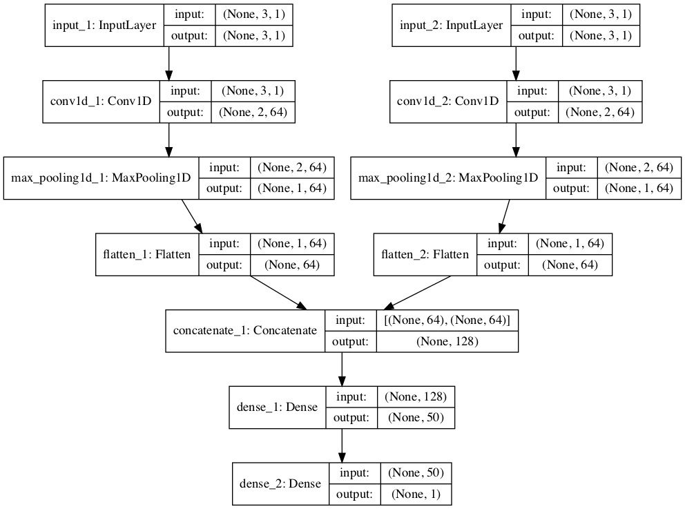
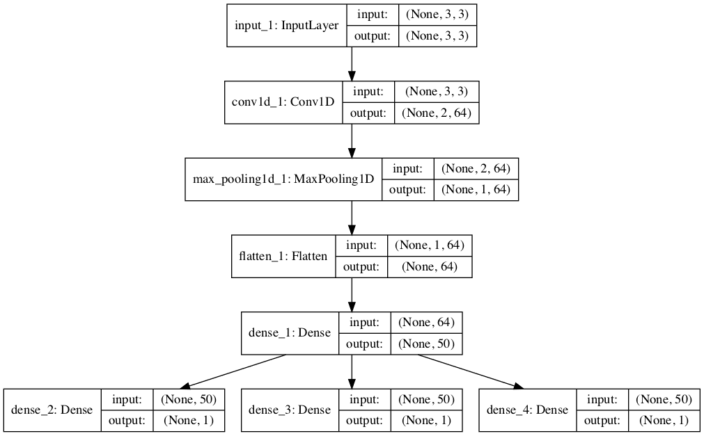


")


Hi Jason,
Good post (as always)!
I got a non related question. Recently I have been developed almost exclusively in javascript (both front react and backend with node js). It has been long time i have done asny solid coding in python, hence my skillset is rusty.
Now, I wonder, how do you see the applying of programming languages for ML apps.
Tensorflow is running now both inn a browser tf.js as well on the backend with node js (just like python?). That sounds like a great thing – one language for everything. There are also courses on the topic, getting more traction
https://www.udemy.com/machine-learning-with-javascript/
Is javascript enough for machine learning apps? or python should be used? Can you please elaborate?
thanks and regards
JSman
Hmmm, maybe for small apps.
I cannot imagine being able to convince my team that a JS solution would make more sense, unless the existing system was all JS or it as a front-end demo or something. Or maybe if the model was fit using something fast and used to make predictions in JS.
Really, you want to use the same tech stack as the rest of the existing system/enterprise.
Dear @Dr.Jason Brownlee,
thank you for sharing your very useful information and codes.
similar to the @JSman, i have done my work on a different platform(i mean Matlab) instead of Python language.
this is my time series prediction code that uses CNN, LSTM, and MLP Net.
please visit my code from my Mathworks account from the link below:
https://www.mathworks.com/matlabcentral/fileexchange/69506-time-series-prediction
This is a common question that I answer here:
https://machinelearningmastery.com/faq/single-faq/can-you-read-review-or-debug-my-code/
Hi Jason,
A very high quality article for me to learn more about deep learning. It really help me a lots.Please keep sharing the knowledge. Thank you!
Cheer
Thanks, I’m glad to hear that.
Thank you so much for such an informative article, I have learnt a lot.
You’re welcome.
Nice site. Just a comment. IMO, It’s a bit pretentious and weak to put the title PhD after your name (” I’m Jason Brownlee PhD…”). You don’t need to validate yourself through a useless degree. You have already earned the respect of all of us through your wonderful work. A mention of your credentials at a bio page would have sufficed. Just my two cents.
Thanks for the feedback.
Testing showed me that “phd” splashed around helps with creditability for first time visitors.
Dr. Brownlee,
My wife has an MS in Robotics Engineering and is a Registered Professional Engineer. I have a PhD in physics from UT. I Know how hard we both worked for our credentials and I certainly would not call them useless. You earned your credentials BRAVO.
Armando
Agreed. Completing degree a degree not useless, although it may not be required to be a practitioner in a given field (e.g. applied machine learning).
How to increase the number of prediction???? Where in code plz tell
What do you mean by the number of prediction, do you mean time steps?
If so, you can start with one of the multi-step forecasting examples and adapt it for your needs.
Thanks Jason for your new clear, detailed and very well explained explanation (as always)!.
I’m glad it helped.
Hi Thanks for this wonderful article.
Please help me to understand when we can use LSTMs and CNNs for Time series forecasting?
I think the best way is to test out both. It is hard to tell which works on what scenarios. But you can think in this way: CNN is memoryless and look at a window at once, but LSTM is stateful with cell state and hidden state built up as you feed in the data. Which one sounds more reasonable for your data? That might be the choice you want to explore first.
I index an image by a low-level feature (color) as form of a digital vector can i can exploit the current topic for an image clasifier
Maybe.
Thanks Jason for a very detailed explanation of CNN, and the many ways we can approach a time forecasting problem with CNNs.
I’m happy it helped.
Hi Jason,
I have become a fan, after reading this post of yours.
I have been trying to use 1D CNNs for one of my network anomaly applications, but somehow couldn’t get them to work effectively.
This post has all that I need to get my network up and running.
Thanks.
I’m happy to hear that!
Hi Jason
Your books and posts have been very helpful in igniting my interest in machine learning. I just started learning deep learning and would like to know your approach on generating rain forecast maps given a data set with images (in gif format) of historical precipitation maps. Seeing as the sequence of past observations are images and not numbers like the examples above how would one prepare the image data.(I’m very new to deep learning)
Perhaps you can use a CNN-LSTM or ConvLSTM to read in the images?
Jason! We can apply RNN-LSTM to the structured data too, what is the edge of using CNN for multivariate timeseries prediction?
No, RNNs are for sequence prediction:
https://machinelearningmastery.com/when-to-use-mlp-cnn-and-rnn-neural-networks/
Your site is pure gold and It is becoming my reference! You are making difference, thanks for educating for us. I became a ML engineer now because your hardwork, thanks again!
Thanks, I’m glad it helps.
Awesome Jason!
I would like to know your opinion on this :
CNN architecture : Input ->Conv1d->Dropout->Conv1d . (There is no Dense Layer, as you noticed!)
Purpose : Multistep Time series Forecasting. For example, 20 “past” input -> 3 “future” output, (continuous output and input).
Use the structure that gives the best performance.
I generally recommend a Dense layer as the output layer when making predictions so that you can specify the transform and structure of the output.
Thank you for your answer!
In addition, what’s your opinion on using filters in “descending order”,
I mean Input ->Conv1d(40 filters)->Dropout->Conv1d(20 filters)->Dropout->Conv1d(3 filters).
P.S. 40,20, 3 are just random numbers.
Seems odd.
Don’t seek my permission, use the model architecture that gives the best performance.
Thanks for providing all this.
I’ve got a question regarding the input dimension while fitting the model, which in case of Conv1D is [samples, timesteps, features]. Now comparing this with the following article using MLP: https://machinelearningmastery.com/how-to-develop-multilayer-perceptron-models-for-time-series-forecasting/ the dimension becomes [samples, features]. What is the reason for this difference although both models should handel “one dimensional” input?
The CNN must read across subsequences of the input, therefore a 3D input shape is required, much like LSTMs.
With subsequence you mean the timesteps of each given feature, right?
No, for all features.
Hi Jason,
Great article!
After some tests, I believe that I can’t predict the next N sequences since the output y is always dependent on the input x (unless I misunderstood the all concept). If so, what is your advice to predict the next N sequences?
I recommend testing multiple framings of your problem and multiple techniques in order to discover what works best for your specific dataset.
Thanks a lot Dr. Jason. May Allah bless you , we are excited to watch CNN after implementing it to Shampoo Sales Dataset… Do you have any idea to do this.
Yes, you can use the CNN on univariate data, although it will very likely be outperformed by a simple linear model.
Perhaps this post will help:
https://machinelearningmastery.com/how-to-grid-search-deep-learning-models-for-time-series-forecasting/
Hi Jason,
great article, thank you!
I have a question though: could you tell me what the data structure of
X1 = X[:, :, 0].reshape(X.shape[0], X.shape[1], n_features)
X2 = X[:, :, 1].reshape(X.shape[0], X.shape[1], n_features)
in the second example of the multiple input series looks like? As an exercise I’m recreating the code using tensorflow.js and while the code is mostly easy to translate, the data structures in python – a language I’m not really familiar with in detail – often get confusing.
Most of the time you have shown a plain example of the input data, but not in this case. So it’s kind of hard for me to understand how you split the data in detail and what you feed into the two visible parts of the network.
Thanks in advance!
Tom
Hi Tom, here we are extracting the first and second features as separate 3d arrays.
A good place to get started with numpy arrays is here:
https://machinelearningmastery.com/index-slice-reshape-numpy-arrays-machine-learning-python/
Hello Jason,
Thank you for your wonderful tutorials. I have a question (sorry if it looks stupid as I am a beginner), if we have 2 outputs from our NN, is it possible to customize the link of certain nodes from last hidden layer to certain output nodes? e.g. if we have two output nodes and 4 nodes in last hidden layer, is it possible that we link 2 nodes from last hidden layer to a specific node in output layer and other 2 nodes in last hidden layer to the other node in the output layer. If yes, can you refer me to relevant literature? I have drawn a rough sketch here. https://imgur.com/a/w8YnRwq
I’m sure you can, but I don’t have an example sorry.
Perhaps try setting the weights to zero after training?
Thank you very much for your response. Can you please elaborate it a little more? Do you mean by setting certain weights which affect these particular ‘connections’ as zero? and why did you say ‘after training’?
Yes, because I don’t think you can do it other ways (e.g. disable weights). Perhaps you can find a better approach.
if we have excel file with 40000 rows and two column than how i can transform to 2D or 3D array as you have taken just 5 number sequence?
I have a number of tutorials on this, perhaps start here:
https://machinelearningmastery.com/convert-time-series-supervised-learning-problem-python/
Then here:
https://machinelearningmastery.com/faq/single-faq/how-do-i-prepare-my-data-for-an-lstm
i got this error
ValueError: Negative dimension size caused by subtracting 3 from 2 for ‘conv2d_25/convolution’ (op: ‘Conv2D’) with input shapes: [?,200,2,48], [3,3,48,13].
Sorry to hear that, maybe one of these ideas will help:
https://machinelearningmastery.com/faq/single-faq/why-does-the-code-in-the-tutorial-not-work-for-me
Hi,
I’m trying to implement “Multi-Step CNN Model” on a time serie so i’m using a 1D convolutional network.
I use a time sequence of 7 weeks as the number of steps in and 40 weeks as the number of weeks to predict.
Is that a bad idea?
Should the number of steps in always be greater or equal to the number of outputs?
Thanks.
I recommend testing a range of diffrent approaches in order to discover what works best for your specific dataset.
Thank you for the very fast response!
With 7 steps in and 40 steps out I get a good MAPE of about 4%.
Even though its a good error rate, my intuition is telling me that using values in the last 7 weeks to predict values for 40 weeks in the future might not be very believable by the end user of the prediction (forecast). What I mean is that the CNN is trained on patterns in those 7 weeks and then is able to predict the pattern 40 weeks in future?
I may be misinterpreting the whole definitions of the time steps in and out so any clarification from you will be greatly appreciated!
I also tried 40 steps in and 40 steps out which yields a MAPE of about 10-12%.
I think a possible reason is my time series has an upward trend with seasonal spikes every 52 weeks and so when the CNN is training it gets “confused” by the spikes which makes the rest of predictions have a higher error rate. Is there any tricks in CNNs to combat that?
Thank you for taking the time to help me!
Perhaps try scaling the data prior to modeling, or even removing trends prior to modeling, then inverse the transforms before calculating error and compare results.
More on what time steps are here (for LSTMs, but applies directly to 1D CNNs):
https://machinelearningmastery.com/faq/single-faq/what-is-the-difference-between-samples-timesteps-and-features-for-lstm-input
We cannot know what the right amount of input history will be for your problem, you must discover the right amount via experimentation with a robust test harness.
Thank you.
Your web site is probably one of the best online for learning ML!
Thank you!
Hello! I ‘ve been fighting the problem of utilizing the Conv1D for several hours now, and for the life of me, I can’t get it to work no matter what I do. Following your ‘Multivariate CNN’ code, I have a dataset of a pandas data frame of dimension (9666,10) [9 features and the 10th column my y), which I convert to numpy array before I run any further operations, and then use the split_sequences function with n_steps = 3, which gives me X of dimension (9664, 3, 9) and y of (9664,). When I run it gives me the “ValueError: Error when checking target: expected conv1d_25 to have 3 dimensions, but got array with shape (9664, 1)”.
Could you please help me out? I cannot believe it won’t work after so much effort
That is odd, what type of output layer do you have?
It sounds like you might have a decoder output model attached?
Firstly, thanks a lot for prompt assistance!
I was only using the very first 1DConv layer just to check if the input was correct. When I added a Flatten() and then a Dense(1) as the output layer, it worked! I did not know that using only the 1D layer would result in such a strange dimensionality error.
Another question, now that I got it to work: When I use “adam” as the optimizer it works fine, but when I switch it to ‘sgd’ it gives me ‘nan’ as the loss, starting from the very first Epoch, with the above data. What could that be?
Could be exploding gradients:
https://machinelearningmastery.com/how-to-avoid-exploding-gradients-in-neural-networks-with-gradient-clipping/
Hi Jason,
Regarding Conv1D, is there a rule of thumb for figuring out the correct number for filters and kernels?
Thanks.
Not really, see this:
https://machinelearningmastery.com/faq/single-faq/how-many-layers-and-nodes-do-i-need-in-my-neural-network
A great article again. Thank you so much.
If I have a structured data set, such as Titanic data set, is it possible to use 1D convolutional NN to train this dataset? I think it is possible, but I don’t know if it is more feasible and better performance.
oringinal X.shape = (sample, no_features)
reshape X to X.shape = (sample, no_feature, 1)
then use several 1D cnn layers to reduce the size of no_feature, finally use one or two dense layer to do classification.
Your oppions are highly appreciated
No, it would only be appropriate for sequence input. E.g. data with spatial or temporal relationship across input features.
Thank you Jason!
Hi Jason,
I just read a paper about using CNN to tabular data. Please have a look.
https://arxiv.org/pdf/1903.06246v1.pdf
What did you learn from it?
I learned that if the collected data can be transfer into the 2D image data or 2D matrices, we can train them using the pre-trained models. Especially. when we only have a small dataset.
However, in this paper, their transformation is hard to understand. I can’t figure out what the model learned? What are your opinions?
Perhaps contact the author of the paper with your question about their method?
Dear Jason,
Having over thousands of time-series data ( .CSV) will be used for training, for example, intra-day stock prices, I am asked to solve a problem which is to predict if a stock will rise or drop. I have no idea how to start with, says, using RNN or CNN, LSTM? or just simple classifier. Besides, I think I will use the first hour data to predict the trend.
0001.CSV: [D1,D2……, D60] (input), [Min,Max] (Output)(should I say it “y”?)
0002.CSV: [D1,D2……, D60] (input), [Min,Max] (Output)
……
3680.CSV: [D1,D2……, D60] (input), [Min,Max] (Output)
which models above is appropriate to do that? Thanks a lot
Perhaps you can model it across time series as a binary classification problem?
I’d encourage you to explore multiple framings of the problem and test a suite of differnt models.
This might help as a start:
https://machinelearningmastery.com/how-to-develop-a-skilful-time-series-forecasting-model/
Thank you very much
Excuse me, your web page will be apply to my thesis for my reference. Do you have a book for discussion like this learning?
Yes, I cover it in this book:
https://machinelearningmastery.com/deep-learning-for-time-series-forecasting/
Thank you very much for another great post.
I’m confused with the two examples of the Multivariate Multi-Step CNN Models.
You said that the model “predicts the next two time-steps of the output sequence beyond the dataset”.
In the ‘Multiple Input Multi-Step Output’ : “..We would expect the next two steps to be [185, 205]” and in the ‘Multiple Parallel Input and Multi-Step Output’: ‘We would expect the values for these series and time steps to be as follows:[ 90, 95, 185 ] , [ 100, 105, 205].
My question:
In both examples the first expected output value -185 (first example) and [90,95,185] (second example) are part of the dataset (not beyond) and were in the training set, so why we need to ‘predict’ them when the model has seen them?
isn’t it only one time-step prediction of the third feature (the out-seq)?
Hi Jason
Pardon my ignorance, but in the Multivariate CNN Models, I am struggling to understand why the model ignores the prior results of the previous time steps. Is it because CNN is borrowed from an image recognition frame work that we cannot do something like ( I am assuming here that the 2 first columns are independent variables, and the third the dependent one, and each line is 3 time steps.
Input
[ 10 15 25 ]
[ 20 25 45 ]
[ 30 35 ? ] ( not sure what encoding the missing values should take here)
Output
[65]
Thanks
I’m not sure I follow, sorry. Can you elaborate, which example are you referring to exactly?
Thanks for your time: Your example in the section “Multivariate CNN Models”
, shows the structure of 1 data point as :
“If we chose three input time steps, then the first sample would look as follows:”
Input:
1 10, 15
2 10, 15
3 30, 35
Output:
1 65
It seems to me that there is as much to learn, given that the third column is a linear combination of the first 2, from the item 1,2 as there is from the item 3 for that sample. As in the output are all linear combination of columns 1 and 2. But the model dismisses using all the data available ( value 25 for item 1 and value 45 for item 2
) in the model. I thought that letting the network study the linear relationship not only at item 3 but also at item 1 and 2 would improve the results. So I was asking why not using that data structure instead:
Input
10 15 25
20 25 45
30 35 ?
Output
65
instead of just
1 10, 15
2 10, 15
3 30, 35
Output:
1 65
that’s because 10+15 adds no value to getting to know the relationship 30+35=65
while knowing that 10+15=25 at item 1, might help understanding the relationship 30+35=65 for that sample? (I was thinking here in a more general time series case than in this particular example. where for example the residual of 10+15 vs 25 might mean something to the residual of 30+35 vs 65)
Thanks
Sure, you can use any framing of the prediction problem you wish.
The idea of this post is to give you many examples or different framings that you can use as a starting point for your own problem.
Hi Jason,
would it be possible to make the model able to take any input size if you make it fully convolutional, by exchanging the dense layers by a 1×1 convolution?
Then it would not be necessary to fix the input_shape which would make the model be able to do a multi step prediction of a fixed length independent from the input length.
Am I correct with this assumption? If yes why is this never addressed in your tutorials?
Perhaps, but not with Keras – it likes to nail down all shapes and sizes so it can optimize the graph.
hi,jason.thank you for your tutorial. I want to ask you the question that how can we visualize the data after being processing by the pooling layer and a dense layer, and the shape of the processed data.
What do you mean by visualize, do you mean the feature maps themselves?
If so, see this post:
https://machinelearningmastery.com/how-to-visualize-filters-and-feature-maps-in-convolutional-neural-networks/
If you mean the shapes, see this post:
https://machinelearningmastery.com/visualize-deep-learning-neural-network-model-keras/
HI Jason,
In your examples, most multivariate time series are metrics, what if there are categorical and also metrics variables?
Each variable must be prepared prior to modeling.
A categorical var can be encoded as either integer/one hot/embedding. Perhaps try a few approaches and see what works best for your specific dataset?
Thanks. That is really a good hint.
I’m glad it helped.
How would I structure a CNN where I have 5000 samples with 500 timesteps each and there is a binary response variable for each of the timesteps?
I have the following setup but am getting an error – keras doesn’t like the value of my y in model.fit:
n_steps_in, n_steps_out = 500, 500
model = Sequential()
model.add(Conv1D(filters=64, kernel_size=2, activation=’relu’, input_shape=(X_train.shape[1], X_train.shape[2])))
model.add(MaxPooling1D(pool_size=2))
model.add(Flatten())
model.add(Dense(50, activation=’relu’))
model.add(Dense(n_steps_out, name=’output’))
model.compile(loss = ‘binary_crossentropy’, optimizer=’adam’)
model.fit(X_train, y_train, epochs=2000)
ValueError: Error when checking target: expected output to have 2 dimensions, but got array with shape (5000, 500, 1)
For reference, x_train.shape is (5000, 500, 265)
y.train.shape is (5000, 500, 1)
Perhaps this will help you to better understand the input shape:
https://machinelearningmastery.com/faq/single-faq/what-is-the-difference-between-samples-timesteps-and-features-for-lstm-input
Hi Jason,
I use TF version 1.13 (I believe same applies for later versions). I was not able to execute:
from keras.layers.convolutional import Conv1D
from keras.layers.convolutional import MaxPooling1D
this, however, did work:
from keras.layers import Conv1D
from keras.layers import MaxPooling1D
I believe that package ‘convolutional’, isn’t available even in later versions of TF, I may be wrong. It seems that this is a reference to source file rather than the package name.
Great article BTW (as expected 😉
Perhaps update your version of Keras to 2.2.4 or higher?
Hi Jason,
Thank you for the swift response. It was counterintuitive (obviously my assumption doesn’t hold) that TensorFlow (or any other backend implementation) of Keras works only with a default version of Keras with wich TensorFlow (backend itself) comes with.
Based on the assumption above, I haven’t considered updating Keras version without updating TensorFlow. This is why I’ve looked at TensorFlow API (implementation) to find a particular class/package.
Once again thank you!
No problem, happy to hear that you resolved your issue.
instead of sequence of np array as input how can we load csv file input to cnn time forecasting can you tell me???
This post shows you how to load a CSV file:
https://machinelearningmastery.com/load-machine-learning-data-python/
How can we increase the number of predictions like 20 step ahead in future where in code should I change plz tell
You have to change the framing of the prediction problem – the dataset.
Then you can either change the model to predict 20 steps or use the model 20 times recursively for 1 step.
That will be great if above example is using tf.data and keras fit_generator. Thank!
Sorry, I don’t have tutorials on tensorflow directly. Thanks for the suggestion.
I do have many examples of using a fit_generator, you can search the blog.
Just that in practical and performance it should be in tf.data. I am looking for time series data to tf.data to batch, mini batch and window conv1d to fit_generator. Thank for your sharing.
Thanks for the suggestion.
Hi Jason,
This is great. I’m stuck with something though, hoping to seek your help.
Along with the times series, the dataset has features like “holiday_flag”,”day_of_week” etc. I was trying to use these as input features. Can you guide a way ?
You can provide them as additional input variables either as a series (booleans) or a separate input to the model.
Does that help?
Thank you for introducing CNN as tool for Time Series problems.
I am wondering if it is a good choice to use CNN1D for time series problems? When should we consider using CNN1D for time series problems? Should we explore and exhaust other options first before coming to CNN? What should be the intuition for picking CNN on a particular TS problem. and lastly what are the cons of using CNN1D against any other approach. Ofcourse the accuracy of a model should be the deciding factor but given a problem should we avoid CNN and use other tools first?
Great question, I believe this framework will answer it:
https://machinelearningmastery.com/how-to-develop-a-skilful-time-series-forecasting-model/
Hi Jason,
I have to do hourly prediction of energy.I have data for four different states and each state contains 25 years data(25 CSV files). So total 100 csv files.
1. I need to predict energy for next 5 years as I have the data till 2014 from 1990
2. Can I use CNN and LSTM both as LSTM is more suitable for 5 years data.
3. How do clean the data as data from morning 4am to 7pm is the value other than that data is either negative or zero(it contains day light saving data).
4. Can I use drift technique along with CNN and LSTM?
5. How do I read the 4 folders in python.
Regards,
Vijaya
Perhaps try combining all data into one file?
Perhaps test a range of different models to see what works best for your data, using this framework:
https://machinelearningmastery.com/how-to-develop-a-skilful-time-series-forecasting-model
Perhaps dig into the data to see how to best clean it. Impossible for me to say off the cuff.
What do you mean by “drift technique”?
Can we apply this CNN for sensor data prediction(Air pollution) in Internet of things?
Perhaps try it?
Hello Jason,
Thanks for this wonderful article! It’s very useful!
Recently I’ve been working with the models you’ve mentioned in this article
I have a question about the multi headed CNN, sometimes the RMSE for the predictions are low and sometimes very high
The descrepencies are too high, is this common ?
Does the CNN (multi headed) just fit models better sometimes compared to other runs ? Even though all parameters remain the same
Or am i possibly making some error ?
This is common for neural nets generally:
https://machinelearningmastery.com/faq/single-faq/why-do-i-get-different-results-each-time-i-run-the-code
Hello Jason,
Your tutorials are very helpful!
I’ve been playing around with CNN architectures for time series forecasting using 1D convolution networks
You had elaborated on how CNN can be used for multivariate time series data in 2 ways
One with a single 1D neural net and another multi headed CNN arrangement
Recently i read about a multi scale CNN architecture where the idea is simple
Different CNNs are trained using same data but the data is downsized for each CNN
For example one CNN is trained using data available for 4 years
Another CNN is trained using the same data but from years 1-3 and not 4
And then both CNNs are concatenated
I tried to use this idea using multi headed CNN, where each CNN is trained with differently sized input vectors and it did not work ???? it just said vectors should be of same sizes
Can i get help from you regarding this ?
Thank you
Best Regards
Vishnu
Thanks!
Sounds like a great approach.
I don’t have any tutorials on it, but I’d love to write about it in the future.
Hi Jason,
Are you able to estimate the confidence intervals of the forecast values using this approach?
I think you mean prediction intervals right?
If so, not really. This might give you ideas:
https://machinelearningmastery.com/prediction-intervals-for-machine-learning/
Sorry, yes I meant prediction intervals. Thanks for the examples.
No problem!
Hi Jason,
Do you have any intuition about how well this method will work for low signal-to-noise ratio signals?
For some signals you can only see any underlying structure, i.e. the signal, if you do additional processing e.g. FFT.
I am asking before I expend any effort on experimenting.
Thanks,
Michael
No, sorry. Intuition suggests that the more you do up front to expose the signal, the better the model will learn – e.g. the more useful it will be.
I recommend prototyping a model and testing with and without data pre-processing.
Hi Jason,
Thank you for your efforts. Your blogs and books have been really helpful in my Ph.D. degree.
I am performing time-series forecasting where I have 21 features. The 20 features contain numbers between 0 to 30. And 21st feature is related to sale. So, it contains numbers in hundreds. I have 1500 points. 1300 points are used for training and 200 points are used for testing.
My task is to predict the 21st feature. My time-series is stationary. I checked by performing ADF test. Now, I standardized my data before training the deep learning models. I am using multi-head architectures, where each feature is passed as input in different heads, and output of each head was concatenated to predict the 21st feature.
My question is: Multi-head CNN-LSTM is performing better than multi-head LSTM. However, my data-set do not contain any spatial features. Also, multi-head CNN is also performing good (which is mostly used for understanding spatial patterns). Why?
Thanks!
I recommend testing a suite of different models in order to discover what works best for your specific dataset.
Hi Jason,
thanks a lot for the explanation above
i want to implement particle swarm optimization as an optimizer
how can I do it?
This might help to get you started:
http://cleveralgorithms.com/nature-inspired/swarm/pso.html
Hi Jason,
Thank you for the article, was clear and super helpful.
By multi-step prediction, how to choose the kernel size? And, is the optimal kernel size related to the number of the predicted steps (prediction horizon)? For example, if we target on a long prediction horizon, say H=24, does a larger kernel size work better in extracting pattern over a long horizon?
I think the kernel size is probably unrelated to the number of steps to forecast.
I recommend using controlled experiments to test a suite of different configurations and discover what works best.
Hi Jason,
Thanks a lot helping many aspiring deeplearning experts.
Your articles and efforts are really awesome and appreciable.
Want to see articles on image filter using CNN or any other deeplearning algorithms.
Thanks,
Venkatesh B
Thanks.
Perhaps start here for CNNs with image data:
https://machinelearningmastery.com/start-here/#dlfcv
Hi, Good day!
I want to disaggregate appliance level power from total smart meter aggregate reading. I have total active power and reactive power, and also ground truth level (active and reactive power) for each appliance. I have, lets say 4 appliances. So how to design a CNN model for the problem?
I cannot design a model for you. I teach how you can design the model yourself.
Hi Jason,
is it possible to to mix Multi-Headed 1D CNN for Multivariate Time Series Forecasting and LSTM?
Sure, a CNN-LSTM.
Hello,Jason I read what you said, and I feel that it is particularly detailed. I encountered a problem in the task of tone sequence recognition, which made me very troubled. I extracted the Mel cepstrum feature of the audio,the CNN+CTC model is used for recognition, but the recognition result is particularly bad, and there is almost no accuracy rate. I would like to ask you where the problem lies.
These tutorials will help:
https://machinelearningmastery.com/start-here/#better
Hi Jason,
Thanks for your great tutorials. I want to combine multi-head CNN and LSTM. so the concatenation of cnn modules will be input for the LSTM module. but I got error when I concatenate the cnn across axis=0. The model is as follows:
visible1 = Input(shape=(n_steps, n_features))
cnn1 = Conv1D(filters=64, kernel_size=2, activation=’relu’)(visible1)
cnn1 = MaxPooling1D(pool_size=2)(cnn1)
cnn1 = Flatten()(cnn1)
# second input model
visible2 = Input(shape=(n_steps, n_features))
cnn2 = Conv1D(filters=64, kernel_size=2, activation=’relu’)(visible2)
cnn2 = MaxPooling1D(pool_size=2)(cnn2)
cnn2 = Flatten()(cnn2)
# merge input models
merge = concatenate([cnn1, cnn2], axis=0)
#rv = RepeatVector(1)(merge)
lstm = LSTM(50, activation=’relu’, return_sequences=True)(merge)
f_lstm = Flatten()(lstm)
dense = Dense(50, activation=’relu’)(f_lstm)
output = Dense(1)(dense)
model = Model(inputs=[visible1, visible2], outputs=output)
I received this error: Input 0 is incompatible with layer lstm_9: expected ndim=3, found ndim=2
Could you please tell me what is wrong here? I really appreciate your time and help.
I’m eager to help, but I don’t have the capacity to review/debug your code as I get 100s of similar requests each day.
Here are some ideas:
https://machinelearningmastery.com/faq/single-faq/can-you-read-review-or-debug-my-code
Lot of thanks to Jason Brownlee. Your contribution is really great. You have published so many things. I have learnt so many things.
You’re very welcome!
Dear Shohreh,
cnn1 = Conv1D(filters=64, kernel_size=2, activation=’relu’)(visible1)
pool1= MaxPooling1D(pool_size=2)(cnn1)
cnn2 = Conv1D(filters=64, kernel_size=2, activation=’relu’)(visible2)
pool2= MaxPooling1D(pool_size=2)(cnn2)
merge = concatenate([cnn1, cnn2], axis=0) # it might work
or,
merge = concatenate([pool1, poo2], axis=0) # it might work
If you get concatenation related error, you can try with changing ‘axis’ value.
Great tip!
Hi Jason,
thanks for your supports!
I want to implement a temperature estimation for an electric motor using a CNN; a regression problem.
A csv file contains all measurements, which are sampled at 2 Hz. The data set consists of 12 columns: 8 columns as input data (such as current, voltage, speed, …) and other 4 columns as output data or targets (the temperature of different parts of the motor).
My question is, should this problem be considered as a time series forecasting? and if yes, how should be the shape of the input data for a CNN?
I ask it because we know, time series forecasting is the use of a model to predict future values based on previously observed values. While regression analysis is often employed in such a way that the current values of the independent time series (inputs) affect the current value of another time series (outputs).
Thank you in advance for your attention.
This will help you shape the data – e.g. the same as you would for an LSTM:
https://machinelearningmastery.com/faq/single-faq/what-is-the-difference-between-samples-timesteps-and-features-for-lstm-input
Great article Jason. Do you have any insights on how these kinds of convents for forecasting, like even WaveNet, compare to RNNs seq-seq in terms of general forecasting performance?
One of the advantages of this is that we can have a variable length sequence as opposed to RNNs. But from what I see on Kaggle though, seq-to-seq RNNs, and Amazon’s Forecasting model (deep AR) is with RNNs. This makes me think that RNNs always dominate over CNNs for time series forecasting. Thoughts?
It is different for each model and each dataset -better to use controlled experiments for your problem rather than talk in useless generalities.
In my experiments, I see CNNs and CNN-LSTM hybrids perform better than vanilla LSTMs.
Hi Jason,
Hope you’re well. I’m enjoying reading your timeseries forecasting articles and I have two questions, I wonder if you could help in pointing me in the right direction:
1. If I have multiple timeseries that may or may not be related (eg. country ID to population), how would one handle the user ID as a pointer for the existence of a different timeseries? As I would like to have a forecasting model that considers the ID and date to make a prediction, and there may be useful patterns between countries to learn. I’ve created a dataset of 70 days for each country formatted as the following:
(values not real, just an example)
Country ID, day, population
1,1,1000
1,2,1500
…
1,70,50000
2,1,2000
2,2,2500
…
and so on
2. If the above is achieved, how then could one have static geopolitical features also considered as input? eg. if I had the population of the UK for every day of 2019, and then also input the 2019 GDP, population density, % in poverty etc. etc. since these features are static, won’t change for the duration of the experiment, but would help in prediction. Likewise my USA data would also have the same set of related geopolitical features and so on for each country in the dataset
Eg:
Country ID, GDP, density, poverty
1,1000,40.5,12.5
2,2000,20.5,9.5
….
and so on
Is this possible in Keras? I’ve been searching online a lot and I can’t find a related example that achieves either of these two things, or even better both
Would love to hear your thoughts on this,
Thanks,
Jordan
Handling of id’s for time series would happen before/after the model with custom code – e.g. a programming question not a modeling question. Same with dates. The model is/should be unaware of id’s and dates.
Hi Jason,
Thank you for all publications, I have a question,
in_seq1 = array([10, 20, 30, 40, 50, 60, 70, 80, 90]) -> Single sequence
How can we handle multiple sequences,
in_seq1 = array([
[10, 20, 30, 40, 50, 60, 70, 80, 90],
[12, 22, 35, 41, 44, 67, 73, 84, 97],
……………………………
[11, 25, 34, 46, 44, 67, 73, 84, 100]
])
Thank you,
See the example in the above tutorial.
Hi Jason,
I highly appreciate that you can provide the link.
Thank you.
You’re welcome.
Hi Jason,
Let me clear out the problem I am facing,
I have a 500 CSV file containing patient’s CTG scan records as (patient_id, {time})
1000.CSV => { 1000ID, 149, 34,45……….156} likewise I have 500 CSV files.
What I did was, I merge those 500 into single CSV, each row contains a UniqueID and time-series data.
Now I want to process these data and get a predicted output for each record.
Highly appreciate if you can advise me on this.
Thank you,
Perhaps this will give you some ideas:
https://machinelearningmastery.com/time-series-forecasting-supervised-learning/
Hi Jason,
I think I can go with the “Multiple Parallel Series” which is described above.
Any thoughts on that?
Thank you.
Yes.
Hi Jason,
Thank you for the guidance so far, After creating Multivariate Forecasting model, what are the techniques we can use to Evaluate it?
Thank you.
Walk-forward validation:
https://machinelearningmastery.com/backtest-machine-learning-models-time-series-forecasting/
Hi Json,
In “Univariate CNN Models” we train the model with only one input sequence, how we can train our model with multiple sequences (with various time steps) .
Thank you
See the “Multivariate” examples above.
Hi Jason,
Thank you so much for this informative tutorial. I was practising the “Multiple Parallel Series” tutorial for a time series task. and I’m a newbie in CNN. while we develop models using LSTM and RNN we used to normalize the data using methods like min-max. But here It is not mentioned. Do we need to normalize the data before it feeds to the model?
Yes, it can be a good idea to scale data prior to modeling:
https://machinelearningmastery.com/machine-learning-data-transforms-for-time-series-forecasting/
What situation would warrant normalization? Your article says “prefer”, but didn’t clarify when that is needed. thanks.
Good question, see this:
https://machinelearningmastery.com/faq/single-faq/when-should-i-standardize-and-normalize-data
Hi Janon,
Thanks for the great article.
I have predicted solar energy using CNN and XGboost and got 98% accuracy. I have 20 years hourly data. I need to forecast for next 1-5 years. Is there any function in CNN or XGboost like in ARIMA for forecasting.
Please suggest.
Great question, not that I’m aware.
Hi sir,
Thank you for this tutorial. I was trying to do univariate cnn and i’m new to cnn. But, I have a sequence of shape (982, 95).
data.shape = (982, 95)
data[0] is the data for day 1, data[1] is the data for day 2 etc, like that I have 982 days data
With your univariate cnn i feed day 1s data and predicted the last value using the previous 20 values, and the result was good. But i want to feed all the 982 days data as input and predict the value of 982th days last value. How can I do that?
I think that is too many days.
Nevertheless, the 3d input shape for a 1DCNN is the same as an LSTM, this will help:
https://machinelearningmastery.com/faq/single-faq/what-is-the-difference-between-samples-timesteps-and-features-for-lstm-input
Dear Sir,
I have a question regarding the the multi_step prediction but as for classification. My question is what should we consider the output layer? In classification problems the number of nodes in output layer is equal to number of classes we have, in multi-step prediction, the number of nodes in output layer is equal is to the number of steps we want to predict, but what would be the number of nodes for output layer in multi_step prediction for classification problems? would it be the number of classes we have multiply by the number of steps we want to predict? or what it should be?
Thanks a lot for your kind help in advance.
You can use a TimeDistributed wrapper to output one classification per output time step. E.g. a seq2seq type model can be used.
So sorry for spamming, but just for confirming that I understood correctly, the last layer should be coded as : model.add(TimeDistributed(Dense(number of classes), activation=’softmax’))?
or it should be the the number of steps we want to predict? model.add(TimeDistributed(Dense(number of time_steps we want to predict), activation=’softmax’))?
A repeatvector can be used to specify the number of output steps:
https://machinelearningmastery.com/encoder-decoder-long-short-term-memory-networks/
Yes. Try it and see. Prototype and test.
Thank you for your good tutorials,
My dataset is time series based with multi-class. It includes many rows (different results induced by simulation in off-line) and 250 columns. data is a type but it different in time (like Weather). I want to train dataset with lowest time window due to operator needs time for action in real-time. What is your idea?
X=[0.9 0.9 0.9 0.45 0.46 0.46 0.48 0.5 0.5 0.65 …………. 0.8 0.81 0.81 0.8] , data is change in fourth sample. I should train dataset with lowest samples before and after this time.
Regards
You are very welcome Amir! Let me know if I can help with any specific questions regarding the code listings.
or it should be model.add(TimeDistributed(Dense(1), activation=’softmax’))?
Dear Jason,
Is there any possibility to change the order of input dimension in CNN or RNN in time-series prediction problems? I mean in normal condition the order of the 3D input is (sample, time step,features). I would like to know if the input can be re-order as (features, time step, samples)?
Thanks a lot for your kind help in advance.
No.
Even not in (samples ,features, time step ) form?
Hi,
when using Conv1D layers for time series data, do you think batch normalization is problematic? Would it make sense to use it? Thank you
Perhaps try it on your data/model and see if it makes a difference.
In regards to deep belief networks, would we apply same hierarchy just as over level thought?
DBN are no longer an effective method relative to CNNs, I recommend focusing on CNNs when working with image data.
Hi, Amazing tutorial.
I just wanted to ask that in Multiple Parallel Series does the features affect each other or is the prediction of one feature independent of the other features.
Sorry if that was somewhat ambiguous, what I wanted ask is :
if i have multiple time series say [X1, X2, X3, X4] then if using Multiple Parallel Series i predict something like [Y1, Y2, Y3, Y4] would Y1 be dependent upon all the features or just X1.
Thanks
We are modeling assuming that the target values are a function of the input variables, both each variate and lag observations of each variate.
Does that help?
Yes thanks a lot
I will try to add some LSTM layers as well and see how that works.
Again thanks a lot
Good luck!
Great insight, thanks for sharing your knowledge. Does this mean that if I have a feature vector/matrix (X) and my output (y), I do not need to use the time series generator? What sort of data preparation is optimal when considering predictive model for time series not meant for forecasting?
Thanks!
Good question, here are some suggestions for data prep for time series in neural nets:
https://machinelearningmastery.com/machine-learning-data-transforms-for-time-series-forecasting/
I am new to deep learning as such.
1) i want to calculate the MSE for the results. I guess i will put actual values from validation set in one list and results in another. and then find MSE. is there a better way of doing this?
You can use this function:
https://scikit-learn.org/stable/modules/generated/sklearn.metrics.mean_squared_error.html
Hi, thank you for this post.
I have 2 questions.
1. Is there any way to do backtesting or cross-validation of the test set? For example, if I use the multi-step CNN with 1 feature and the output is 30. I want to know how well is the prediction (accuracy) for the first timestep in the future and so on till the 30th time step. I guess I would have to test with several folds (in order). How it should be done?
2. It would be good if as time goes on I add new data to the training or test data (like a rolling window)? It has to be retrained? I ask that because my intuition says that the data near current time would be better for the prediction. I am wrong? However, i do not know if one example (added) is going to make a difference in the short term.
Thank you very much again for your work. It is amazing. Sorry for my english.
Yes, you can use walk-forward validation to evaluate a time series model.
You can find hundreds of examples on the blog, perhaps start here:
https://machinelearningmastery.com/backtest-machine-learning-models-time-series-forecasting/
Yes, you can choose to retrain the model each step or not.
Thank you for your reply! I’ve been reading your other posts and I’ve found them really useful.
However, I still have two more questions:
1. Is there any problem if my training data (predictors or x’s) are binary as well as my labels?
2. It would be correct or not conceptually wrong if for example in your example of using a number of time steps per sample of 3 and then using the same data but with a number of time steps of 6 (when preparing the data)? That way there would be more training examples.
I am looking forward reading your new material soon. One again, thanks.
Thanks!
No, you can have categorical input variables, although that should be encoded, e.g.:
https://machinelearningmastery.com/how-to-prepare-categorical-data-for-deep-learning-in-python/
Sorry, not sure I follow your second question. Perhaps this will help in preparing lag obs as input:
https://machinelearningmastery.com/time-series-forecasting-supervised-learning/
Hi Jason,
Thank you so much for such an informative article
I have 2 questions hopefully you can help me and answer them.
First: I understand that using CNN for time series forecasting required data to be reshaped into (samples, timesteps, features ) however if my model is using (samples, features, timesteps ) what does this means? I am not aware of the theory part, that’s why I am not sure about the difference.
in the experiments, my model gives me more accurate results with the second case!
Second: if I want some feature to be used as it is at some stage of a functional model. Is it possible?
I am asking this because I used one naive model , I found good results. I want to use these results with a combination of the deep learning model. I tried to use the output of the naive model by itself to one layer network with linear function .. but I didn’t get the same result. I want to get the output exactly equals to the input. is it possible? I am sorry if this is a silly question
It means you may have to restructure your data prior to modeling.
You can pass the output of the naive model as input to the deep learning model, or use another model afterward to ensemble the predictions from both models.
Hi Jason, how are you?
I was wondering, if I want to do a multi-step forecast but the labels are binary (1 if sales go up, 0 otherwise) in each step ahead. I have two questions:
1) The last layer should be: model.add(Dense(n_output, activation=’sigmoid’)) or model.add(Dense(n_output, activation=’softmax’))?
2) The loss function should be: ‘binary_crossentropy’ or ‘categorical_crossentropy’?
I do not know how to interpret classes in this problem. Classes are the multi-step forecast or the binary component of 1 if sales go up and 0 otherwise? I hope if possible you can clear it up. Thanks your very much. Have a wonderfull day.
For binary classification you will need to use the sigmoid activation and the binary cross entropy loss function.
Thank you Jason!!!
You’re welcome.
Hi Jason, is there a chance to evaluate the gradient of the function which is approximated by the network with respect to the network input?
Yes, the prediction error from the model calculated using the expected output and the predicted output.
Dear Jason,
Thanks for the tutorial! In the multivariate CNN case, one of the TS can be an exogenous variable like temperature for electricity load ?
Does in make sense in the CNN structure? Or LSTM is better ?
Last question :), can CNN and LSTM can be concatenate?
Thanks a lot, Giulio
You’re welcome.
Yes. Try a number of models and configurations and discover what works best for your specific dataset.
Hi! Thanks for the tutorial.
I am not understanding the very last passage (prediction) of the Multiple Input Series.
#Prediction example
x_input = array([[80, 85], [90, 95], [100, 105]])
print(x_input)
x_input = x_input.reshape(1, n_steps, n_features)
yhat = model.predict(x_input, verbose=0)
print(yhat)
This code gets me the following error:
cannot reshape an array of size 6 into shape (1,3,1)
We have size 6 because we are understandably missing the value we want to predict…
but then which shape should we pass to the predict function if the (1,3,1) is not available?
Thank you very much.
-A
Sorry for the trouble! I solved it. I was passing as n_features 1 instead of 2 .. silly error.
Thank you again for the great tutorial!!
No problem!
Sorry to hear that you are having trouble, these tips may help:
https://machinelearningmastery.com/faq/single-faq/why-does-the-code-in-the-tutorial-not-work-for-me
Hi! Thanks for the tutorial.
I have to model a NN for this problem:
sales forecast of big products. I have a data set for the last 2 years of sales by month with information about country, product code, phase in, phout date, attributes for the product. The data are very sparse for the most part of countryies and product (2 or 3 units by year, country). I have to produce a forecast at month level for the next 24 months, the accuracy of the first 6 months of forecast and in particular the first month are the most important in therms of performance.
Data set: 111.000.000 samples
row sample: month of sale, sale Qty, product Code, market, phase in date, phase out date, product attribute 1, product attribute 2, product attribute 3.
Which approach do you suggest me? Do you have a sample of this kind of problem?
This framework will provide a good starting point:
https://machinelearningmastery.com/how-to-develop-a-skilful-time-series-forecasting-model/
Really great post!
There is another variation of the input and output data I am trying to model and could not find the best match for it.
Suppose we have an individual parallel time series (multiple parallel and multi-step) for each sample. Since the number of samples would be high, it is going to be inefficient to model each one separately. What do you recommend?
Each parallel time series would be a feature, in the [sample, timestep, feature] structure of input data.
hello sir!
I am a big fan of yours and u really make some great tutorials.I strongly suggest u should run a youtube channel.U will have limitless followers.
Thanks for the suggestion, I don’t think video is an effective way to learn/practice applied machine learning, it is too passive:
https://machinelearningmastery.com/faq/single-faq/do-you-have-videos
Hi Jason, Thank you so much for this amazing article. Your articles are always helpful.
My regression model takes 10 time steps as an input and predicts next two time steps. But during training validation accuracy is more than the training accuracy. And I don’t seem to find the solution for the same. Could you may be give some inputs what might be wrong? what should I look into?
Thanks in advance.
You’re welcome.
Perhaps these tips will help:
https://machinelearningmastery.com/start-here/#better
Specifically:
https://machinelearningmastery.com/introduction-to-regularization-to-reduce-overfitting-and-improve-generalization-error/
Hi Jason,
Huge thanks for these tutorials! They have been of huge help in understanding the topic in greater detail.
I am wondering if it is possible to train a multivariate model on multiple datasets? I am trying to train the model on impulse response datasets.
Any input would be greatly appreciated.
David
Sure.
You could combine all data into one dataset and fit a model.
You could fit the model on each dataset in turn, saving/loading between datasets or keeping the model in memory.
Some combination of the above two methods.
Thanks for the demo. I found it helpful.
Splitting sequences and put them into ever growing X and y lists subsequently converting them into a 3D array is extremely slow and inefficient, especially for large datasets. It is much faster to pre-allocate the fixed size of the 3D array and populate the array in the loop.
Yes, it is just an example of the models, not of efficient data prep.
Hello,
I have a problem similar to what you explained in “Multiple Input Multi-Step Output” and I have a doubt about what you reported. Referencing to your data
[[ 10 15 25]
[ 20 25 45]
[ 30 35 65]
[ 40 45 85]
[ 50 55 105]
[ 60 65 125]
[ 70 75 145]
[ 80 85 165]]
I have a similar structure where the third column represents my target. If we consider each row of the “matrix” as the data related to a particular timestamp, I’ve prepared my input data (I will show only the X_1 for simplicity) as follow:
[ 10 15 25]
[ 20 25 45]
[ 30 35 65] —> y_1 (target): 85 or [85,105] according to if I want a single forecast or multi-step forecast.
I’ve used also the third column in input as they represent past values which I know and it makes sense to use, but I think you didn’t use it to give a general example. Practically, at level code I used the same approach you explained in “Multiple Input Multi-Step Output”, changing only the seq_y as seq_y = sequences[end_ix:out_end_ix, -1] in your split_sequences function in order to specify the target I want.
I don’t understand why, in your example, you consider 65 as the first desired output. In my opinion 65 represents a “current” value not a future value I’m going to predict, the future value/s I want to predict are those related to following timestamps which are 85 and/or [85, 105]. Did you choose [65, 85] as output to give a general example, as I suppose?
Thanks a lot in advance.
You can frame the data any way you like. The examples in this tutorials are to motivate the models only.
Perhaps this will help:
https://machinelearningmastery.com/time-series-forecasting-supervised-learning/
Hello Jason,
Thank you for the great tutorial. I used your multivariate CNN model above, but I have a problem:
When I choese “n_steps” as 1 or two I have a problem of “Negative dimension size caused by subtracting 2 from 1 for ‘{{node max_pooling1d_137/MaxPool}} = MaxPool[T=DT_FLOAT, data_format=”NHWC”, explicit_paddings=[], ksize=[1, 2, 1, 1], padding=”VALID”, strides=[1, 2, 1, 1]](max_pooling1d_137/ExpandDims)’ with input shapes: [?,1,1,64].”
I need to choose “n_steps” as 1, can you help me please. Thank you.
Yes, the model may need to be adjusted to support very small input sequences, or you may need to use larger sequences if the model is left unchanged.
Hi Jason:
I would like to be sure if I understood the concept well… CNNs were originally created for the treatment of images and image sequences (video), which are 2D data (rows and columns); where the CNN preserves the spatial structure of the input data and is invariant with the object position and the distortion of the same, in other words, a CNN predicts better the structure of the data with respect to space.
In the case of CNNs for time series, a type of CNN 1D is used, but does this CNN 1D model retain this advantage of preserving the spatial structure of the data in its extraction of characteristics, as if it were image sequences?
Thanks for your attention.
Correct.
Yes, 1D CNN has similar properties, although applied to a 1d sequence of observations.
Ok thank you understood then, and this raises three more questions about it:
• If instead of using a 2D CNN on an image, the image is flattened by converting the pixels into a 1D vector, could a 1D CNN be used with this image and the same forecast results could be achieved as with a 2D CNN, that is, would the spatial structure of the data be preserved in the same way as in the image?
• If, on the other hand, I have a multivariate time series organized in 2D (rows and columns), with values other than pixels, could I apply a 2D CNN as if it were an image and could I achieve a regression forecast for each field of the dataset, where the spatial structure of the data is preserved, or would there be a risk that being a 2D CNN, the dataset is always interpreted as pixel values (between 0 and 255)?
• Are there any advantages of faster convergence between a 1D CNN and a 2D CNN?
Thanks for your attention.
Working with pixels instead of raw sequence data will be worse in every way (my opinion).
A 1D CNN can operate on multivariate sequence data directly, a 2d CNN is inappropriate (again, my opinion).
Run experiments to confirm if you like.
It was your opinion from experience precisely what I wanted. Thanks for your answer.
You’re welcome.
Hi Jason:
This publication seems excellent to me, thank you very much for your work. Could you tell me where I can consult information or what I should do to know how to optimize the configuration of a 1D CNN model for the case of multiple parallel input and multi-step output type, so that I can adapt this model to my own case study of multivariate time series forecast ?.
Thanks for your attention.
Thanks for the very informative tutorial.
you discussed an idea for the implementation of cnn1 and cnn2 and then the merging of features from these two models to predict the output, my small query is – can we use the same idea for lstm1 and lstm2 ?
Sure.
CNN model is giving error for time_step=1. The error is “Negative dimension size caused by subtracting 2 from 1 for ‘conv1d_1/convolution/Conv2D’ (op: ‘Conv2D’) with input shapes: [?,1,1,5], [1,2,5,64]”.
How can I rectify this error, if I don’t want to increase the number of time step?
My above mentioned error is rectified by some reshaping in input data. i.e.
I interchanged the rows and column. means initially input.shape[1] was n_step and input.shape[2] was features, after reshaping input.shape[2] became n_step and input.shape[1] became features. Then I applied convolution on my data.
But now my question is- Is it logically correct or not? If not then what else can I do?
Not really, see this (e.g. data shape for 1d cnn’s is the same as for lstms):
https://machinelearningmastery.com/faq/single-faq/what-is-the-difference-between-samples-timesteps-and-features-for-lstm-input
Perhaps try smaller kernel sizes or fewer layers until you discover the specific cause of the issue.
Hi Jason:
Could you tell me where I can consult information or what I should do to know how to optimize the configuration of a 1D CNN model for the case of multiple parallel input and multi-step output type, so that I can adapt this model to my own case study of multivariate time series forecast ?.
Thanks for your attention.
These tutorials will help you tune a neural net:
https://machinelearningmastery.com/start-here/#better
Hı Jason
Can you please help me i have items (item1 …..itemn)
And i have sequences like
Seq1[item1……item10]
Seq2[item1……item10]
.
.
.
Seqn[item1……item10]
İtems are not numbers or words .. like songs names contain both numbers and character I want to predict the next item item11 for each sequence and I want the predicted items to be from the whole dataset (all items ) I’m using convolutional neural networks and embedding please tell how can I do that !!(prediction from the whole dataset ) and how can I reshape my sequences to use them ( should I use sliding window and how ? Or should I take the last item from every sequence like output ).. please
and thank you for all what you do .
This will help, where each embedding vector is a “feature vector”:
https://machinelearningmastery.com/faq/single-faq/what-is-the-difference-between-samples-timesteps-and-features-for-lstm-input
I can’t understand, can you please explain more?
No problem, which part would you like me to explain?
I use the nine first items of sequences as inputs X and the last item as output y … I reshape the X to be [9 , 9 100] the size of the the item vector after embedding is 100 … I fed the inputs to my CNN model with input shape of (9,100) … And I put a finale dense layer with output of shape 100 ( size of vector ) … I’m going right ?
If the embedding has a length of 100, then the number of features input to the CNN or LSTM model would be 100, e.g. [?, ?, 100].
If you have 9 time steps per sample, then the shape would be [?, 9, 100]
And when I put the input shape to (9,100) it works but predict the same values
Perhaps the model requires tuning of the architecture and learning hyperparameters:
https://machinelearningmastery.com/start-here/#better
i have input data with shape (985, 9, 100) .. i put input shape [985 , 9 , 100 ] it did not work and i try input shape [None ,9, 100] it did not work too
i get this error ValueError: Input 0 of layer max_pooling1d_4 is incompatible with the layer: expected ndim=3, found ndim=4. Full shape received: [None, 985, 3, 100]
this is my model
model_CNN = Sequential()
model_CNN.add(Conv1D(filters=100, kernel_size=3, activation=’relu’ , input_shape=(None, 9 ,100)))
model_CNN.add(Conv1D(filters=100, kernel_size=3, activation=’relu’))
model_CNN.add(Dropout(0.25))
model_CNN.add(Conv1D(filters=100, kernel_size=3, activation=’relu’))
model_CNN.add(MaxPooling1D(pool_size=2))
model_CNN.add(Dropout(0.25))
model_CNN.add(Flatten())
model_CNN.add(Dense(200 , activation=’relu’))
model_CNN.add(Dense(100))
model_CNN.compile(optimizer=’adam’, loss=’mse’)
this is my input X shape (985, 9, 100)
and my output y shape (985, 100)
i’m really sorry, i’m beginner and i really need to deal with that
Sorry, the cause of the issue is not clear.
Perhaps work with one or two rows of data and the simplest model in order to debug the cause of the issue.
Thanks for your tutorial. A new paper by Stanford professors “Deep Learning Statistical Arbitrage” https://papers.ssrn.com/sol3/papers.cfm?abstract_id=3862004 uses a CNN with transformer to predict residual stock returns. Could you write about transformers?
Thanks for the suggestion.
Hi Jason:
The following question arises for me, when working with the deep learning methods MPL, CNN, LSTM or their hybrids for the forecast of a time series of the multiple parallel input and multi-step output type, the forecast that these methods perform for each one of the time steps for each of the variables, do they take into account the correlation of each of the other variables in addition to the autocorrelation with the variable that is being predicted, or not?
Thanks for your attention.
The model may or may not take into account specific properties in the training dataset. We don’t have direct control over the statistical patterns used by a neural net model.
Ok, thanks for that clarification.
Thanks for a detailed explanation Dr. Jason. I am in the need of your sincere suggestion regarding a work that I am doing now for prediction of data.
I am using CNN regression model without a pooling layer. This is so since the purpose of pooling is to merge semantically similar features into one; however, feature images represent one geologic phenomenon, and none of these geologic phenomena will be the same as those in the real world.
I could not get an appropriate R2 accuracy value.: Training is about 71 and testing is about 54%. Could you please suggest how to improve? By the way, I am using 24 data points as training since we don’t have more data points. Need your sincere suggestion.
Perhaps some of the suggestions here will help:
https://machinelearningmastery.com/start-here/#better
Hi Jason:
I wish you could help me with something. I am trying to configure a 1D CNN, to forecast a multivariate time series with multiple parallel input and multi-step output. It is clear to me that finding the best configuration is basically achieved by trial and error, but I have made some attempts and I cannot find at least an initial configuration that gives me the basis and from there I begin to carry out trials and errors.
I want to train the network with approximately 77400 samples each one composed of a Xwith 10 time steps as input and a y with 3 tiem steps as output.
Could you please tell me as a first test how robust that network must be? That is, initially how many convolutional layers a network must have for this amount of data, more or less with how many filters and with what kernel size it must have , as well as how many initial nodes should the dense layer have, the possible number of epochs or the batch size.
I repeat, I know that reaching a complete adjustment is done by trial and error more than anything, but I hope you understand that what happens is that I do not know how to size it sufficiently for a first test according to the amount of data; and since the possibilities are too many, I would really appreciate it if you can help me to size it enough for a first test according to the amount of data, answering those questions. Because this would already help me to have a perspective on what dimensions of that network I should move to do tests.
Thanks for your attention.
We cannot know what configuration will work well or best for a given prediction problem, I recommend testing a suite of methods and compare results to naive methods.
Consider scaling the data and consider a large number of architectures. Ensure you’re using a robust test harness, e.g. walk-forward validation, perhaps repeated.
Hi Jason:
I would like to ask you, I understand that when working with 1D CNN it is better to work with raw data, that is, how they are without scaling them or doing a normalization or standardization process, is that right ?; or is there a rule or something similar to know if it is better to do any of those processes to my data to use a 1D CNN?
Thanks for your attention.
Normalizing and standardizing may still necessary in that case if you do not want to see a large input range. Remember, in sigmoidal function, for example, the function works best only on a small range around zero. If your input is in a scale of billions, it may take a long time for the gradient descent algorithm to converge. If you know that it will not be that case in your data, then you’re right.
Thanks for the explanation, it was just what I needed. According to this, in a case where the raw data with a range of values between 0 and 10 it may be better not to pass the data through normalization or standardization. Is it so?
Thanks for your attention.
These tutorials are really helpful. I need LSTM out-of-sample forecast example on univariate, did you work on this?
Yes, there are many examples on the blog, perhaps start here:
https://machinelearningmastery.com/make-predictions-long-short-term-memory-models-keras/
Hi Jason:
I would like to know your opinion, if I want to use a 1D CNN model, an MLP or one of the LSTM models to perform forecasting on a time series of the Multiple Parallel Input and Multi-step Output type, whose data have values that only go from 0 to 10 ; Would it be more convenient to carry out some kind of scaling, standardization or standardization of the data?
Thanks for your attention.
These are data preprocessing techniques, which applies to the input data. If your input data has any reason these techniques are useful (e.g., one feature is in range of 0 to 0.001 while another feature is in range of 0 to 10), then you need them. The output range is controlled by the output layer of the network. Hence should not need the scaler for output data.
That is, in the case that all the data have the same range of values such as integers (0,1,2,3,4,5,6,7,8,9,10), there would not be a Real need to apply this type of technique to the input data to use 1D CNN, MLP and LSTM neural networks?
Thank you for your attention, I remain pending.
For data like that I am quite comfortable without any scaler. A scaler is to help make the convergence faster. A MLP for example, if we initialize the weight using standard normal and using tanh as the activation function. The convergence would be faster if the input data is within -1 to +1 (because the initial value is already in its ball park range) than 5000 to 8000 (which needs a lot of iterations to move the weight to this range).
Ok Adrian, thanks for the explanation, it is very helpful to me.
Hello Adrian:
I would like to know your opinion, if as I told you in the previous question in the case that all the data have the same range of values such as integers (0,1,2,3,4,5,6,7,8, 9,10), in a multivariate series; and you want to make a future forecast of the Multiple Parallel Input and Multi-step Output type, but where the series in question is sparse type, that is, it has many values at zero. Do you think that in this case it would be convenient to carry out some type of processing to the input data such as the ones we have already discussed (scaling, normalization, standardization) or some other such as PSA, etc.
This to use 1D CNN, MLP and LSTM neural networks; and Random Forest.
Thank you for your kind attention, I remain attentive.
You need to try that out to confirm if it is helpful. But usually, sparse data is not good for StandardScaler because the variance is obviously underestimated. Otherwise, it should not do harm than not having the preprocessing.
Thanks, as always Adrian, your help is very useful for me.
You’re welcomed.
Hello Jason, thanks a lot for all your posts
I’m working on a MultiStep-Multivariate CNN for demand forecasting with vector Output (48 setps in, 12 steps output).
¿Is there an easy way to visualize the loss on the Train data? For example like you did on the One-Step LSTM for AirLine Passengers.
¿How can I plot a train validation-loss-curve? Just want to make sure about the right amount of epochs
Regards
Yes, you may need to capture the values yourself in a list/array and plot manually at the end of training.
Thank you very much for your wonderful sharing! I would like to ask if there is any CNN-LSTM model for probability prediction?
This one may give you an introduction, but I believe you can easily make up your own model once you know about the concept of how to do it: https://machinelearningmastery.com/cnn-long-short-term-memory-networks/
Jason,
First of all thank you for great blog. I’ve learn a lot from your articles.
I would like ask you for advice in regarding Multiple Parallel Series.
I have case where my data came from 5 probes and they has been noted in this way that if there is a peak in signal it is marked as 1, if there aren’t peak there is 0.
My goal is to predict potential peak in each probe.
Examples can be found below.
Two questions.
1. As you can observe in each step in series there are only two 1 in row. This is some kind of additional knowledge that should be taken by neural network to predict results.
Question. Did this CNN Multiple Parallel Series example what you provided takes knowledge also from others parallel series?
2. Is it for this Boolean data what I have this CNN Multiple Parallel Series is the best way to analyze ?
p1 p2 p3 p4 p5
Step 1 0 1 0 0 1
Step 2 0 1 0 1 0
Step 3 1 0 0 0 1
Step 4 0 1 0 1 0
Step 5 0 1 1 0 0
Step 6 0 1 0 0 1
Step 7 0 0 1 0 1
Step 8 0 1 0 0 1
Step 9 1 1 0 0 0
Step 10 0 0 0 1 1
Step 11 1 0 0 0 1
Step 12 0 1 0 0 1
Step 13 0 1 1 0 0
Step 14 0 1 0 0 1
Step 15 0 1 0 0 1
Thank you,
Marcin
For (2) Boolean should not be a problem, but you may not want to use MaxPooling1D as you are almost always get 1 from it. AveragePooling1D may be what you want. For (1) I think you are talking about using p1 to p5 together as input and each of them is a time series. In this case, you are not developing a 1D convolution but 2D one. More like the case of image.
Hello Adrian and Jason:
I would like to know your opinion, if as I told you in the previous question in the case that all the data have the same range of values such as integers (0,1,2,3,4,5,6,7,8, 9,10), in a multivariate series; and you want to make a future forecast of the Multiple Parallel Input and Multi-step Output type, but where the series in question is sparse type, that is, it has many values at zero. Do you think that in this case it would be convenient to carry out some type of processing to the input data such as the ones we have already discussed (scaling, normalization, standardization) or some other such as PSA, etc.
This to use 1D CNN, MLP and LSTM neural networks; and Random Forest.
Thank you for your kind attention, I remain attentive.
Thanks for the great tutorial
The kernel size=2 means a kernel of 2*2 matrix; Similarly, kernel size=3 means 3*3.
What if I want to take a kernel matrix 1*3 or 1*2? How can I get this matrix? I saw some research papers on CNN considering a kernel size of 1*3, 1*4…. so on.
If I am taking the code kernel_size=(1,3), I got an error “The
kernel_sizeargument must be a tuple of 1 integer. Received: (1, 3).”In the examples here, it is Conv1D, which is a 1xN matrix. What you described are for Conv2D, which are more often seen from examples of image problems.
you are giving input shape as [timesteps,1] in univariate time series prediction. how will the model predict for other samples/rows in the dataset. like if I have timesteps of 3 for 400 samples
X-sample1 -> 1 2 3
X-sample2 -> 2 3 4
and so on
since we are passing just 1 sample , how are other samples passed for training or does it automatically recognizes?
And the model summary showing output parameter as None signifies what? how will we compute output size with this?
Hi SHG…The following may be of interest to you in terms of understanding prediction in general:
https://machinelearningmastery.com/how-to-make-classification-and-regression-predictions-for-deep-learning-models-in-keras/
So, I’m hoping to have a discussion on the suitability of the use of CNNs for time series regression modelling.
I first noticed that all the CNN, CNN-LSTM and ConvLSTM models from your book were unable to model volatile nature for energy demand. I plotted the predictions against the ground truth and saw that the predictions were basically flat lines compare to the real demand as if the model could capture the higher frequencies. I’ve seen a similar thing in other papers that use CNN in their architecture. The model only seems to get the general shape. Sure you could say that the models are small, there wasn’t a lot of data but I’ve seen the same thing in the results of other papers that use CNN in their architectures.
I’ve read that CNNs are known to reduce noise(ie reduce high frequencies) . I get that it is impossible to model the noise or randomness but could this be a limitation of CNN or is there something I don’t understand or that I’m not accounting for?
Does the neural network only fit to the patterns that exist and that its architecture allows and everything else is just noise?
Hi Corne…Please clarify your question so that we may better assist you.
Hello. Thank you for your useful content
I have a question, are there any examples of this for R software ??
Because according to your code, I wrote the code in R software, but I have a problem in compiling the model.
Can you guide me?
Hi Kia…I would highly recommend the following resource:
https://machinelearningmastery.com/machine-learning-with-r/
Hi Jason,
Thank you so much for your useful content. I have 2 questions,
1.How to find MAPE for measurement. (code python).
2. How to Split Train Data Set and Test Data Set for Univariate Time series data.
Thank you so much.
Hi Belle…the following resources may be of interest:
1. https://www.statology.org/mape-python/
2. https://towardsdatascience.com/time-series-from-scratch-train-test-splits-and-evaluation-metrics-4fd654de1b37
Hi Jason,
Great work as usual.
Please, do you anticipate developing any Wavenet / Temporal CN code example?
Thanks and regards,
Alex
Hi Alecesa…We do not currently have content related to those topics. The following is a complete list of our ebooks:
https://machinelearningmastery.com/products/
Hi Jason
Thanks for your info
Please can you help me for any examples to optimize conv1d using automatic or intelligence tuning hyper prameter for conv1d bulging with keras
Such as
Examples about
1-pso-cnn1d
2-kerasga -conv1d by using pygad package
Thanks
Hi Sandra…The following resource may add clarity:
https://www.kdnuggets.com/2020/05/hyperparameter-optimization-machine-learning-models.html
Thanks ????
I need another question
I ask if it Is possible with Keras to use Conv2d to perform a Conv1d? The question may seem weird, but I need to use a tool have conv2d
Such as I have raw dataset and x-training =(14322,23)
I need to use this code to enter raw data for x training above instead of using this data in code for image (100,100,3)
If possible what changes in input and other prameter???
# Build the keras model using the functional API.
inout laver = tensorflow.keras.layers.Input(shape=(100, 100, 3))
con laver1 = tensorflow.keras.lavers.Conv2D(filters=5,
kernel_size=7,
activation=”relu”) (input_layer)
max_pool1 = tensorflow.keras.layers.MaxPooling2D(pool_size=(5,5),
strides=5) (conv_layer1)
con laver2 = tensorflow.keras.lavers.Conv2D(filters=3,
kernel size=3
con_layer2 = tensorflow.keras.layers.Conv2D(filters=3,
kernel size=3
activation=”relu”) (max_pool1)
flatten laver= tensorflow.keras.layers.Flatten()(conv_layer2)
dense_layer = tensorflow.keras.layers.Dense (15, activation=”relu”) (flatten_layer)
output_layer = tensorflow.keras.layers.Dense(4, activation=”softmax”) (dense laver) model = tensorflow.keras.Model(inputs=input_layer, outputs=output_layer)
Jason,
Thank you for a great article.
I am trying to determine at a glance if a Keras model is fully connected or not.
It seems the rule of thumb is if none of the layers are Dense, then the model is NOT fully connected.
For my univariate time series, if a 1D convolution auto encoder model only uses Keras layers that are 1D conv, Dropout, and 1D conv transpose, how do you tell if the model is fully connected or not ?
I am using data with time and voltage to model in an autoencoder. None of the layers are Dense, but what specifically makes a Keras model NOT fully connected ?
Hi Chuck…You are very welcome! The following resource may add clarity:
https://towardsdatascience.com/coding-a-convolutional-neural-network-cnn-using-keras-sequential-api-ec5211126875#:~:text=Keras%20Dense%20class&text=In%20Keras%2C%20these%20layers%20are,using%20multiple%20fully%20connected%20layers.
Thanks ????
I need another question
I ask if it’s possible to use Conv2d to perform a Conv1d? The question may seem weird, but I need to use a tool that Used conv2d
If possible how ???
Such as i need to use this code for raw dataset have
X-training =(14255,23) instead of datay for image (100,100,3)
What changes in input and other parameters? If possible
# Build the keras model using the functional API.
Input layer = tensorflow.keras.layers.Input(shape=(100, 100, 3))
con laver1 = tensorflow.keras.lavers.Conv2D(filters=5,
kernel_size=7,
activation=”relu”) (input_layer)
max_pool1 = tensorflow.keras.layers.MaxPooling2D(pool_size=(5,5),
strides=5) (conv_layer1)
con laver2 = tensorflow.keras.lavers.Conv2D(filters=3,
kernel size=3
Jason – thank you so much for this tutorial – it was a God-send for me. Unlike some tutorials, clearly meant to enable, with brief, clear explanations where people are likely to need them, and with the logical progression in scale from the simplest examples to the more complex using the same basic framework. This is how it should be done when educating! It is so very much appreciated.
Thank you tfrud for your support and feedback! We greatly apprecite it!
The best and the most detailed set of tutorials for any kind of models we search! This is so perfect, thanks!
Hi Ragav…Thank you for your feedback and support! We appreciate your kind words!
Hey James, since you have put input_shape=(n_steps, n_features) in the CNN model architecture, is there a need to reshape X to be: X = X.reshape((X.shape[0], X.shape[1], n_features))?. I have tried a similar approach as yours without reshaping X, and the CNN model have worked. Meanwhile when i have tried putting input_shape=(n_steps,) I got an error that the model expects 3D input.
Hi Levi…
Thank you for your question regarding the input shape in CNN models for time series forecasting!
**Understanding Input Shapes in CNN for Time Series**
When working with Convolutional Neural Networks (CNNs) for time series forecasting using frameworks like Keras (TensorFlow backend), it’s crucial to ensure that your input data is correctly shaped to match the expectations of the convolutional layers.
**Expected Input Shape for
Conv1DLayers:**– The
Conv1Dlayer expects a **3D input** with shape:(batch_size, steps, features)
– **
batch_size**: The number of samples in a batch (handled automatically during training).– **
steps**: The number of time steps (sequence length).– **
features**: The number of features at each time step.– In your model definition, when you specify:
python
input_shape=(n_steps, n_features)
you’re informing Keras that each sample has a shape of
(n_steps, n_features), excluding the batch size.**Reshaping Input Data:**
– If your input data
Xis not already in the required 3D shape, you **need to reshape it**.– For example, if
Xhas shape(samples, n_steps), andn_features=1(univariate time series), you need to reshape it to(samples, n_steps, n_features):python
X = X.reshape((X.shape[0], X.shape[1], n_features))
– This reshaping adds an additional dimension to represent the features at each time step.
**Why Did Your Model Work Without Reshaping
X?**– **Possible Reasons:**
– **X Already Had the Correct Shape**: If your input data
Xwas already in the shape(samples, n_steps, n_features), there was no need to reshape it.– **Default Behavior with Single Feature**: In some cases, if
n_features=1and your data is in shape(samples, n_steps), Keras might implicitly treat it as(samples, n_steps, 1). However, this behavior is not guaranteed and can lead to inconsistencies.**Error with
input_shape=(n_steps,):**– When you specify
input_shape=(n_steps,), you’re indicating that each sample has shape(n_steps,), which is **2D** when including the batch dimension.– The
Conv1Dlayer **requires a 3D input**, so Keras raises an error because it expects an input shape of(batch_size, steps, features).**Error Message Example:**
ValueError: Input 0 of layer "conv1d" is incompatible with the layer: expected ndim=3, found ndim=2.
**Correct Usage:**
– Always include the
n_featuresdimension in yourinput_shape.– Reshape your input data accordingly.
**Example Steps:**
1. **Prepare Your Data:**
pythonimport numpy as np
# Example data
samples = 100 # Number of samples
n_steps = 10 # Number of time steps
n_features = 1 # Number of features
# Generate dummy data
X = np.random.rand(samples, n_steps)
# Original shape
print('Original shape:', X.shape) # (100, 10)
2. **Reshape Input Data:**
python# Reshape to include the features dimension
X = X.reshape((X.shape[0], X.shape[1], n_features))
# New shape
print('Reshaped X:', X.shape) # (100, 10, 1)
3. **Define the Model:**
pythonfrom tensorflow.keras.models import Sequential
from tensorflow.keras.layers import Conv1D, Flatten, Dense
model = Sequential()
model.add(Conv1D(filters=64, kernel_size=2, activation='relu', input_shape=(n_steps, n_features)))
model.add(Flatten())
model.add(Dense(50, activation='relu'))
model.add(Dense(1))
model.compile(optimizer='adam', loss='mse')
# Model summary
model.summary()
4. **Train the Model:**
python# Generate dummy target variable
y = np.random.rand(samples, 1)
# Train the model
model.fit(X, y, epochs=10, verbose=1)
**Key Points to Remember:**
– **3D Input Requirement**:
Conv1Dlayers require a 3D input. Ensure your data matches this requirement.– **Reshaping Is Necessary When**:
– Your data is not already in 3D shape.
– You have a univariate time series and need to add the features dimension.
– **Specifying
input_shapeCorrectly**:– Use
input_shape=(n_steps, n_features)forConv1Dlayers.– Do not omit the
n_featuresdimension, even if it’s 1.**Why Specifying
input_shape=(n_steps,)Causes an Error:**– The
input_shapeparameter defines the shape **excluding** the batch size.–
input_shape=(n_steps,)implies each sample has shape(n_steps,), which is 1D.– Including the batch size, the model expects input of shape
(batch_size, n_steps), which is 2D.–
Conv1Dlayers cannot process 2D inputs; they need 3D inputs.**Additional Insights:**
– **Why Your Model Worked Without Reshaping in Some Cases**:
– If your data pipeline or dataset already included the features dimension, explicit reshaping wasn’t necessary.
– Some layers might internally add a dimension if possible, but relying on this can lead to unexpected behavior.
– **Best Practices**:
– **Always Explicitly Reshape**: To avoid confusion and ensure compatibility, always reshape your input data to match the expected input shape of your model layers.
– **Consistent Data Shapes**: Maintain consistency in data shapes throughout your model to prevent errors.
**Troubleshooting Tips:**
– **Verify Data Shapes**:
python

  print('X shape:', X.shape)

  print('y shape:', y.shape)
– **Check Model Input Expectations**:
python

  print('Expected input shape:', model.input_shape)
– **Common Errors**:
– **Mismatch in Expected Dimensions**: Ensure the dimensions of your input data match the
input_shapespecified in your model.– **Incorrect Reshaping**: Double-check the order and values used in reshaping.
**Conclusion:**
– **Reshaping is Necessary**: Unless your data is already in the correct 3D shape, you need to reshape it to match the expected input of the
Conv1Dlayer.– **Include All Dimensions**: Always specify all required dimensions in your
input_shape, including the features dimension.– **Understand Layer Requirements**: Different layers have different input requirements; understanding these will help you design models without errors.
**References:**
– [Keras Conv1D Documentation](https://keras.io/api/layers/convolution_layers/convolution1d/)
– [Time Series Forecasting with CNNs](https://machinelearningmastery.com/how-to-use-convolutional-neural-networks-for-time-series-forecasting/)
Thank you very much Jason,
I have been following for a long time and also reading the text book. I was seeking your help in determining the kernel size for a time-series.
In the text book, you mention that the kernel size is equal to the number of time steps (” The kernel size is the number of time steps included of each read operation of the input sequence”/ pg. 131 Section 9.2.5).
However, I see in most examples that despite the raw_seq haing n_steps = 3, we use a kernel size of 2.
Can you help me understand the intuition behind kernel size selection?
Great question, Hossam! In time-series convolutional models, the kernel size determines the number of time steps included in each read operation of the input sequence. Here’s a deeper look into the intuition behind kernel size selection:
1. **Kernel Size as Lookback Window**: Think of the kernel size as the “lookback window” for the model. A kernel size of 2, for example, means the model will examine two consecutive time steps at a time, allowing it to capture short-term dependencies. Larger kernel sizes allow the model to see further back in time per filter step, capturing longer dependencies.
2. **Flexibility vs. Complexity**: Smaller kernels (e.g., kernel size = 2) focus on immediate or short-term changes between adjacent time steps, making them effective for detecting finer-grained patterns. Larger kernel sizes (matching or exceeding the time steps) increase the model’s capacity to learn broader temporal patterns but add computational complexity. Often, selecting a smaller kernel, like 2 or 3, is a practical balance.
3. **Experimentation and Data-Driven Choice**: While some guidelines suggest setting the kernel size close to or matching
n_steps, it’s common to experiment to see which kernel size best captures the time-based patterns in your data. It’s about finding a sweet spot between overfitting and adequately capturing temporal dynamics.In short, the kernel size doesn’t strictly need to match
n_steps; it can be smaller to enable more nuanced feature extraction, especially in shorter-term patterns.