Multilayer Perceptrons, or MLPs for short, can be applied to time series forecasting.
A challenge with using MLPs for time series forecasting is in the preparation of the data. Specifically, lag observations must be flattened into feature vectors.
In this tutorial, you will discover how to develop a suite of MLP models for a range of standard time series forecasting problems.
The objective of this tutorial is to provide standalone examples of each model on each type of time series problem as a template that you can copy and adapt for your specific time series forecasting problem.
In this tutorial, you will discover how to develop a suite of Multilayer Perceptron models for a range of standard time series forecasting problems.
After completing this tutorial, you will know:
How to develop MLP models for univariate time series forecasting.
How to develop MLP models for multivariate time series forecasting.
How to develop MLP models for multi-step time series forecasting.
Kick-start your project with my new book Deep Learning for Time Series Forecasting, including step-by-step tutorials and the Python source code files for all examples.
Let’s get started.
How to Develop Multilayer Perceptron Models for Time Series Forecasting Photo by Bureau of Land Management, some rights reserved.
Tutorial Overview
This tutorial is divided into four parts; they are:
Univariate MLP Models
Multivariate MLP Models
Multi-Step MLP Models
Multivariate Multi-Step MLP Models
Univariate MLP Models
Multilayer Perceptrons, or MLPs for short, can be used to model univariate time series forecasting problems.
Univariate time series are a dataset comprised of a single series of observations with a temporal ordering and a model is required to learn from the series of past observations to predict the next value in the sequence.
This section is divided into two parts; they are:
Data Preparation
MLP Model
Data Preparation
Before a univariate series can be modeled, it must be prepared.
The MLP model will learn a function that maps a sequence of past observations as input to an output observation. As such, the sequence of observations must be transformed into multiple examples from which the model can learn.
Consider a given univariate sequence:
1
[10, 20, 30, 40, 50, 60, 70, 80, 90]
We can divide the sequence into multiple input/output patterns called samples, where three time steps are used as input and one time step is used as output for the one-step prediction that is being learned.
1
2
3
4
5
X, y
10, 20, 30 40
20, 30, 40 50
30, 40, 50 60
...
The split_sequence() function below implements this behavior and will split a given univariate sequence into multiple samples where each sample has a specified number of time steps and the output is a single time step.
1
2
3
4
5
6
7
8
9
10
11
12
13
14
# split a univariate sequence into samples
def split_sequence(sequence,n_steps):
X,y=list(),list()
foriinrange(len(sequence)):
# find the end of this pattern
end_ix=i+n_steps
# check if we are beyond the sequence
ifend_ix>len(sequence)-1:
break
# gather input and output parts of the pattern
seq_x,seq_y=sequence[i:end_ix],sequence[end_ix]
X.append(seq_x)
y.append(seq_y)
returnarray(X),array(y)
We can demonstrate this function on our small contrived dataset above.
The complete example is listed below.
1
2
3
4
5
6
7
8
9
10
11
12
13
14
15
16
17
18
19
20
21
22
23
24
25
26
27
# univariate data preparation
from numpy import array
# split a univariate sequence into samples
def split_sequence(sequence,n_steps):
X,y=list(),list()
foriinrange(len(sequence)):
# find the end of this pattern
end_ix=i+n_steps
# check if we are beyond the sequence
ifend_ix>len(sequence)-1:
break
# gather input and output parts of the pattern
seq_x,seq_y=sequence[i:end_ix],sequence[end_ix]
X.append(seq_x)
y.append(seq_y)
returnarray(X),array(y)
# define input sequence
raw_seq=[10,20,30,40,50,60,70,80,90]
# choose a number of time steps
n_steps=3
# split into samples
X,y=split_sequence(raw_seq,n_steps)
# summarize the data
foriinrange(len(X)):
print(X[i],y[i])
Running the example splits the univariate series into six samples where each sample has three input time steps and one output time step.
1
2
3
4
5
6
[10 20 30] 40
[20 30 40] 50
[30 40 50] 60
[40 50 60] 70
[50 60 70] 80
[60 70 80] 90
Now that we know how to prepare a univariate series for modeling, let’s look at developing an MLP model that can learn the mapping of inputs to outputs.
Need help with Deep Learning for Time Series?
Take my free 7-day email crash course now (with sample code).
Click to sign-up and also get a free PDF Ebook version of the course.
MLP Model
A simple MLP model has a single hidden layer of nodes, and an output layer used to make a prediction.
We can define an MLP for univariate time series forecasting as follows.
Important in the definition is the shape of the input; that is what the model expects as input for each sample in terms of the number of time steps.
The number of time steps as input is the number we chose when preparing our dataset as an argument to the split_sequence() function.
The input dimension for each sample is specified in the input_dim argument on the definition of first hidden layer. Technically, the model will view each time step as a separate feature instead of separate time steps.
We almost always have multiple samples, therefore, the model will expect the input component of training data to have the dimensions or shape:
1
[samples, features]
Our split_sequence() function in the previous section outputs the X with the shape [samples, features] ready to use for modeling.
Once the model is defined, we can fit it on the training dataset.
1
2
# fit model
model.fit(X,y,epochs=2000,verbose=0)
After the model is fit, we can use it to make a prediction.
We can predict the next value in the sequence by providing the input:
1
[70, 80, 90]
And expecting the model to predict something like:
1
[100]
The model expects the input shape to be two-dimensional with [samples, features], therefore, we must reshape the single input sample before making the prediction, e.g with the shape [1, 3] for 1 sample and 3 time steps used as input features.
1
2
3
4
# demonstrate prediction
x_input=array([70,80,90])
x_input=x_input.reshape((1,n_steps))
yhat=model.predict(x_input,verbose=0)
We can tie all of this together and demonstrate how to develop an MLP for univariate time series forecasting and make a single prediction.
Running the example prepares the data, fits the model, and makes a prediction.
Note: Your results may vary given the stochastic nature of the algorithm or evaluation procedure, or differences in numerical precision. Consider running the example a few times and compare the average outcome.
We can see that the model predicts the next value in the sequence.
1
[[100.0109]]
Multivariate MLP Models
Multivariate time series data means data where there is more than one observation for each time step.
There are two main models that we may require with multivariate time series data; they are:
Multiple Input Series.
Multiple Parallel Series.
Let’s take a look at each in turn.
Multiple Input Series
A problem may have two or more parallel input time series and an output time series that is dependent on the input time series.
The input time series are parallel because each series has an observation at the same time step.
We can demonstrate this with a simple example of two parallel input time series where the output series is the simple addition of the input series.
We can reshape these three arrays of data as a single dataset where each row is a time step and each column is a separate time series. This is a standard way of storing parallel time series in a CSV file.
Running the example prints the dataset with one row per time step and one column for each of the two input and one output parallel time series.
1
2
3
4
5
6
7
8
9
[[ 10 15 25]
[ 20 25 45]
[ 30 35 65]
[ 40 45 85]
[ 50 55 105]
[ 60 65 125]
[ 70 75 145]
[ 80 85 165]
[ 90 95 185]]
As with the univariate time series, we must structure these data into samples with input and output samples.
We need to split the data into samples maintaining the order of observations across the two input sequences.
If we chose three input time steps, then the first sample would look as follows:
Input:
1
2
3
10, 15
20, 25
30, 35
Output:
1
65
That is, the first three time steps of each parallel series are provided as input to the model and the model associates this with the value in the output series at the third time step, in this case 65.
We can see that, in transforming the time series into input/output samples to train the model, that we will have to discard some values from the output time series where we do not have values in the input time series at prior time steps. In turn, the choice of the size of the number of input time steps will have an important effect on how much of the training data is used.
We can define a function named split_sequences() that will take a dataset as we have defined it with rows for time steps and columns for parallel series and return input/output samples.
Running the example first prints the shape of the X and y components.
We can see that the X component has a three-dimensional structure.
The first dimension is the number of samples, in this case 7. The second dimension is the number of time steps per sample, in this case 3, the value specified to the function. Finally, the last dimension specifies the number of parallel time series or the number of variables, in this case 2 for the two parallel series.
We can then see that the input and output for each sample is printed, showing the three time steps for each of the two input series and the associated output for each sample.
1
2
3
4
5
6
7
8
9
10
11
12
13
14
15
16
17
18
19
20
21
22
23
(7, 3, 2) (7,)
[[10 15]
[20 25]
[30 35]] 65
[[20 25]
[30 35]
[40 45]] 85
[[30 35]
[40 45]
[50 55]] 105
[[40 45]
[50 55]
[60 65]] 125
[[50 55]
[60 65]
[70 75]] 145
[[60 65]
[70 75]
[80 85]] 165
[[70 75]
[80 85]
[90 95]] 185
Before we can fit an MLP on this data, we must flatten the shape of the input samples.
MLPs require that the shape of the input portion of each sample is a vector. With a multivariate input, we will have multiple vectors, one for each time step.
We can flatten the temporal structure of each input sample, so that:
1
2
3
[[10 15]
[20 25]
[30 35]]
Becomes:
1
[10, 15, 20, 25, 30, 35]
First, we can calculate the length of each input vector as the number of time steps multiplied by the number of features or time series. We can then use this vector size to reshape the input.
1
2
3
# flatten input
n_input=X.shape[1]*X.shape[2]
X=X.reshape((X.shape[0],n_input))
We can now define an MLP model for the multivariate input where the vector length is used for the input dimension argument.
When making a prediction, the model expects three time steps for two input time series.
We can predict the next value in the output series proving the input values of:
1
2
3
80, 85
90, 95
100, 105
The shape of the 1 sample with 3 time steps and 2 variables would be [1, 3, 2]. We must again reshape this to be 1 sample with a vector of 6 elements or [1, 6]
We would expect the next value in the sequence to be 100 + 105 or 205.
Note: Your results may vary given the stochastic nature of the algorithm or evaluation procedure, or differences in numerical precision. Consider running the example a few times and compare the average outcome.
Running the example prepares the data, fits the model, and makes a prediction.
1
[[205.04436]]
There is another more elaborate way to model the problem.
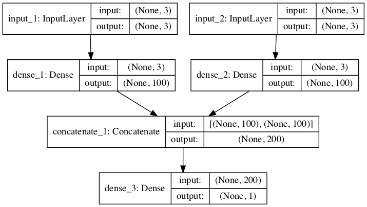
Each input series can be handled by a separate MLP and the output of each of these submodels can be combined before a prediction is made for the output sequence.
We can refer to this as a multi-headed input MLP model. It may offer more flexibility or better performance depending on the specifics of the problem that are being modeled.
First, we can define the first input model as an MLP with an input layer that expects vectors with n_steps features.
1
2
3
# first input model
visible1=Input(shape=(n_steps,))
dense1=Dense(100,activation='relu')(visible1)
We can define the second input submodel in the same way.
1
2
3
# second input model
visible2=Input(shape=(n_steps,))
dense2=Dense(100,activation='relu')(visible2)
Now that both input submodels have been defined, we can merge the output from each model into one long vector, which can be interpreted before making a prediction for the output sequence.
The image below provides a schematic for how this model looks, including the shape of the inputs and outputs of each layer.
Plot of Multi-Headed MLP for Multivariate Time Series Forecasting
This model requires input to be provided as a list of two elements, where each element in the list contains data for one of the submodels.
In order to achieve this, we can split the 3D input data into two separate arrays of input data: that is from one array with the shape [7, 3, 2] to two 2D arrays with the shape [7, 3]
1
2
3
# separate input data
X1=X[:,:,0]
X2=X[:,:,1]
These data can then be provided in order to fit the model.
1
2
# fit model
model.fit([X1,X2],y,epochs=2000,verbose=0)
Similarly, we must prepare the data for a single sample as two separate two-dimensional arrays when making a single one-step prediction.
1
2
3
x_input=array([[80,85],[90,95],[100,105]])
x1=x_input[:,0].reshape((1,n_steps))
x2=x_input[:,1].reshape((1,n_steps))
We can tie all of this together; the complete example is listed below.
Note: Your results may vary given the stochastic nature of the algorithm or evaluation procedure, or differences in numerical precision. Consider running the example a few times and compare the average outcome.
Running the example prepares the data, fits the model, and makes a prediction.
1
[[206.05022]]
Multiple Parallel Series
An alternate time series problem is the case where there are multiple parallel time series and a value must be predicted for each.
For example, given the data from the previous section:
1
2
3
4
5
6
7
8
9
[[ 10 15 25]
[ 20 25 45]
[ 30 35 65]
[ 40 45 85]
[ 50 55 105]
[ 60 65 125]
[ 70 75 145]
[ 80 85 165]
[ 90 95 185]]
We may want to predict the value for each of the three time series for the next time step.
This might be referred to as multivariate forecasting.
Again, the data must be split into input/output samples in order to train a model.
The first sample of this dataset would be:
Input:
1
2
3
10, 15, 25
20, 25, 45
30, 35, 65
Output:
1
40, 45, 85
The split_sequences() function below will split multiple parallel time series with rows for time steps and one series per column into the required input/output shape.
Running the example first prints the shape of the prepared X and y components.
The shape of X is three-dimensional, including the number of samples (6), the number of time steps chosen per sample (3), and the number of parallel time series or features (3).
The shape of y is two-dimensional as we might expect for the number of samples (6) and the number of time variables per sample to be predicted (3).
Then, each of the samples is printed showing the input and output components of each sample.
1
2
3
4
5
6
7
8
9
10
11
12
13
14
15
16
17
18
19
20
(6, 3, 3) (6, 3)
[[10 15 25]
[20 25 45]
[30 35 65]] [40 45 85]
[[20 25 45]
[30 35 65]
[40 45 85]] [ 50 55 105]
[[ 30 35 65]
[ 40 45 85]
[ 50 55 105]] [ 60 65 125]
[[ 40 45 85]
[ 50 55 105]
[ 60 65 125]] [ 70 75 145]
[[ 50 55 105]
[ 60 65 125]
[ 70 75 145]] [ 80 85 165]
[[ 60 65 125]
[ 70 75 145]
[ 80 85 165]] [ 90 95 185]
We are now ready to fit an MLP model on this data.
As with the previous case of multivariate input, we must flatten the three dimensional structure of the input data samples to a two dimensional structure of [samples, features], where lag observations are treated as features by the model.
1
2
3
# flatten input
n_input=X.shape[1]*X.shape[2]
X=X.reshape((X.shape[0],n_input))
The model output will be a vector, with one element for each of the three different time series.
1
n_output=y.shape[1]
We can now define our model, using the flattened vector length for the input layer and the number of time series as the vector length when making a prediction.
We can predict the next value in each of the three parallel series by providing an input of three time steps for each series.
1
2
3
70, 75, 145
80, 85, 165
90, 95, 185
The shape of the input for making a single prediction must be 1 sample, 3 time steps and 3 features, or [1, 3, 3]. Again, we can flatten this to [1, 6] to meet the expectations of the model.
Note: Your results may vary given the stochastic nature of the algorithm or evaluation procedure, or differences in numerical precision. Consider running the example a few times and compare the average outcome.
Running the example prepares the data, fits the model, and makes a prediction.
1
[[100.95039 107.541306 206.81033 ]]
As with multiple input series, there is another, more elaborate way to model the problem.
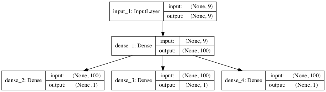
Each output series can be handled by a separate output MLP model.
We can refer to this as a multi-output MLP model. It may offer more flexibility or better performance depending on the specifics of the problem that is being modeled.
First, we can define the input model as an MLP with an input layer that expects flattened feature vectors.
1
2
3
# define model
visible=Input(shape=(n_input,))
dense=Dense(100,activation='relu')(visible)
We can then define one output layer for each of the three series that we wish to forecast, where each output submodel will forecast a single time step.
1
2
3
4
5
6
# define output 1
output1=Dense(1)(dense)
# define output 2
output2=Dense(1)(dense)
# define output 2
output3=Dense(1)(dense)
We can then tie the input and output layers together into a single model.
To make the model architecture clear, the schematic below clearly shows the three separate output layers of the model and the input and output shapes of each layer.
Plot of Multi-Output MLP for Multivariate Time Series Forecasting
When training the model, it will require three separate output arrays per sample.
We can achieve this by converting the output training data that has the shape [7, 3] to three arrays with the shape [7, 1].
1
2
3
4
# separate output
y1=y[:,0].reshape((y.shape[0],1))
y2=y[:,1].reshape((y.shape[0],1))
y3=y[:,2].reshape((y.shape[0],1))
These arrays can be provided to the model during training.
1
2
# fit model
model.fit(X,[y1,y2,y3],epochs=2000,verbose=0)
Tying all of this together, the complete example is listed below.
Note: Your results may vary given the stochastic nature of the algorithm or evaluation procedure, or differences in numerical precision. Consider running the example a few times and compare the average outcome.
Running the example prepares the data, fits the model, and makes a prediction.
1
2
3
[array([[100.86121]], dtype=float32),
array([[105.14738]], dtype=float32),
array([[205.97507]], dtype=float32)]
Multi-Step MLP Models
In practice, there is little difference to the MLP model in predicting a vector output that represents different output variables (as in the previous example) or a vector output that represents multiple time steps of one variable.
Nevertheless, there are subtle and important differences in the way the training data is prepared. In this section, we will demonstrate the case of developing a multi-step forecast model using a vector model.
Before we look at the specifics of the model, let’s first look at the preparation of data for multi-step forecasting.
Data Preparation
As with one-step forecasting, a time series used for multi-step time series forecasting must be split into samples with input and output components.
Both the input and output components will be comprised of multiple time steps and may or may not have the same number of steps.
For example, given the univariate time series:
1
[10, 20, 30, 40, 50, 60, 70, 80, 90]
We could use the last three time steps as input and forecast the next two time steps.
The first sample would look as follows:
Input:
1
[10, 20, 30]
Output:
1
[40, 50]
The split_sequence() function below implements this behavior and will split a given univariate time series into samples with a specified number of input and output time steps.
Running the example splits the univariate series into input and output time steps and prints the input and output components of each.
1
2
3
4
5
[10 20 30] [40 50]
[20 30 40] [50 60]
[30 40 50] [60 70]
[40 50 60] [70 80]
[50 60 70] [80 90]
Now that we know how to prepare data for multi-step forecasting, let’s look at an MLP model that can learn this mapping.
Vector Output Model
The MLP can output a vector directly that can be interpreted as a multi-step forecast.
This approach was seen in the previous section were one time step of each output time series was forecasted as a vector.
With the number of input and output steps specified in the n_steps_in and n_steps_out variables, we can define a multi-step time-series forecasting model.
The model can make a prediction for a single sample. We can predict the next two steps beyond the end of the dataset by providing the input:
1
[70, 80, 90]
We would expect the predicted output to be:
1
[100, 110]
As expected by the model, the shape of the single sample of input data when making the prediction must be [1, 3] for the 1 sample and 3 time steps (features) of the input and the single feature.
1
2
3
4
# demonstrate prediction
x_input=array([70,80,90])
x_input=x_input.reshape((1,n_steps_in))
yhat=model.predict(x_input,verbose=0)
Tying all of this together, the MLP for multi-step forecasting with a univariate time series is listed below.
Note: Your results may vary given the stochastic nature of the algorithm or evaluation procedure, or differences in numerical precision. Consider running the example a few times and compare the average outcome.
Running the example forecasts and prints the next two time steps in the sequence.
1
[[102.572365 113.88405 ]]
Multivariate Multi-Step MLP Models
In the previous sections, we have looked at univariate, multivariate, and multi-step time series forecasting.
It is possible to mix and match the different types of MLP models presented so far for the different problems. This too applies to time series forecasting problems that involve multivariate and multi-step forecasting, but it may be a little more challenging, particularly in preparing the data and defining the shape of inputs and outputs for the model.
In this section, we will look at short examples of data preparation and modeling for multivariate multi-step time series forecasting as a template to ease this challenge, specifically:
Multiple Input Multi-Step Output.
Multiple Parallel Input and Multi-Step Output.
Perhaps the biggest stumbling block is in the preparation of data, so this is where we will focus our attention.
Multiple Input Multi-Step Output
There are those multivariate time series forecasting problems where the output series is separate but dependent upon the input time series, and multiple time steps are required for the output series.
For example, consider our multivariate time series from a prior section:
1
2
3
4
5
6
7
8
9
[[ 10 15 25]
[ 20 25 45]
[ 30 35 65]
[ 40 45 85]
[ 50 55 105]
[ 60 65 125]
[ 70 75 145]
[ 80 85 165]
[ 90 95 185]]
We may use three prior time steps of each of the two input time series to predict two time steps of the output time series.
Input:
1
2
3
10, 15
20, 25
30, 35
Output:
1
2
65
85
The split_sequences() function below implements this behavior.
Running the example first prints the shape of the prepared training data.
We can see that the shape of the input portion of the samples is three-dimensional, comprised of six samples, with three time steps and two variables for the two input time series.
The output portion of the samples is two-dimensional for the six samples and the two time steps for each sample to be predicted.
The prepared samples are then printed to confirm that the data was prepared as we specified.
1
2
3
4
5
6
7
8
9
10
11
12
13
14
15
16
17
18
19
20
(6, 3, 2) (6, 2)
[[10 15]
[20 25]
[30 35]] [65 85]
[[20 25]
[30 35]
[40 45]] [ 85 105]
[[30 35]
[40 45]
[50 55]] [105 125]
[[40 45]
[50 55]
[60 65]] [125 145]
[[50 55]
[60 65]
[70 75]] [145 165]
[[60 65]
[70 75]
[80 85]] [165 185]
We can now develop an MLP model for multi-step predictions using a vector output.
Running the example fits the model and predicts the next two time steps of the output sequence beyond the dataset.
We would expect the next two steps to be [185, 205].
Note: Your results may vary given the stochastic nature of the algorithm or evaluation procedure, or differences in numerical precision. Consider running the example a few times and compare the average outcome.
It is a challenging framing of the problem with very little data, and the arbitrarily configured version of the model gets close.
1
[[186.53822 208.41725]]
Multiple Parallel Input and Multi-Step Output
A problem with parallel time series may require the prediction of multiple time steps of each time series.
For example, consider our multivariate time series from a prior section:
1
2
3
4
5
6
7
8
9
[[ 10 15 25]
[ 20 25 45]
[ 30 35 65]
[ 40 45 85]
[ 50 55 105]
[ 60 65 125]
[ 70 75 145]
[ 80 85 165]
[ 90 95 185]]
We may use the last three time steps from each of the three time series as input to the model and predict the next time steps of each of the three time series as output.
The first sample in the training dataset would be the following.
Input:
1
2
3
10, 15, 25
20, 25, 45
30, 35, 65
Output:
1
2
40, 45, 85
50, 55, 105
The split_sequences() function below implements this behavior.
Running the example first prints the shape of the prepared training dataset.
We can see that both the input (X) and output (Y) elements of the dataset are three dimensional for the number of samples, time steps, and variables or parallel time series respectively.
The input and output elements of each series are then printed side by side so that we can confirm that the data was prepared as we expected.
1
2
3
4
5
6
7
8
9
10
11
12
13
14
15
16
17
18
19
20
21
22
(5, 3, 3) (5, 2, 3)
[[10 15 25]
[20 25 45]
[30 35 65]] [[ 40 45 85]
[ 50 55 105]]
[[20 25 45]
[30 35 65]
[40 45 85]] [[ 50 55 105]
[ 60 65 125]]
[[ 30 35 65]
[ 40 45 85]
[ 50 55 105]] [[ 60 65 125]
[ 70 75 145]]
[[ 40 45 85]
[ 50 55 105]
[ 60 65 125]] [[ 70 75 145]
[ 80 85 165]]
[[ 50 55 105]
[ 60 65 125]
[ 70 75 145]] [[ 80 85 165]
[ 90 95 185]]
We can now develop an MLP model to make multivariate multi-step forecasts.
In addition to flattening the shape of the input data, as we have in prior examples, we must also flatten the three-dimensional structure of the output data. This is because the MLP model is only capable of taking vector inputs and outputs.
Running the example fits the model and predicts the values for each of the three time steps for the next two time steps beyond the end of the dataset.
We would expect the values for these series and time steps to be as follows:
1
2
90, 95, 185
100, 105, 205
Note: Your results may vary given the stochastic nature of the algorithm or evaluation procedure, or differences in numerical precision. Consider running the example a few times and compare the average outcome.
We can see that the model forecast gets reasonably close to the expected values.
In this tutorial, you discovered how to develop a suite of Multilayer Perceptron, or MLP, models for a range of standard time series forecasting problems.
Specifically, you learned:
How to develop MLP models for univariate time series forecasting.
How to develop MLP models for multivariate time series forecasting.
How to develop MLP models for multi-step time series forecasting.
Do you have any questions?
Ask your questions in the comments below and I will do my best to answer.
Develop Deep Learning models for Time Series Today!
Great article! Well written and learned a lot. I am trying to work on my own project now but am a bit stuck trying to integrate categorical variables into this. I think I want to create a univariate multistep MLP however for each sample there are a few categorical variables. Can I turn this into a multivariate multistep problem. For example, suppose I have two separate stores (store A and store B) and the history of sales for each store over the past few years and I want to predict the next month.
Could I generate multivariable samples as so:
[10, A]
[20, A]
[30, A]
[40, A]
…
[100,A]
Hey your blog help me a lot as I am researching using neural network to predict a specific model. I just have a question about this paper. In the beginning you have a sequence of data which you can use split sequence command, but what if I have a column/list of data, how do I split my data?
Thank you
with open(‘testfile.txt’) as inputfile:
for line in inputfile:
raw_seq.append(line.strip().split(‘,’))
#print (raw_seq)
…
look_for = raw_seq[len(raw_seq)-n_steps_in:len(raw_seq)]
x_input = array(look_for)
, it gives me this error
”
File “C:\Users\AppData\Local\Programs\Python\Python36\lib\site-packages\keras\engine\training_utils.py”, line 127, in standardize_input_data
‘with shape ‘ + str(data_shape))
ValueError: Error when checking input: expected dense_1_input to have 2 dimensions, but got array with shape (6, 1, 1)
”
Please, how can we proceed in this case:
Time series: [2 4 6 0 1 3 5 0 6 7 8 0], we find that after every 3 values it returns to 0.
Logically, we must have this feature in the prediction like [2 4 6 0 1 3 5 0 6 7 8 0 V1 V2 V3 0 V’1 …]
What should I do?
Do I make the prediction until I get this! Or is there a parameter to define?
Hello Jason Brownlee! I want to express my profound gratitude to you! Just by following your short crash course I’ve learnt soo much. Thank you and keep up the good work!
I have a question : is there a way to make a trained model to predict more number of values than the number of values it was trained with?
Using the multivariate-multi-step example, the model was trained with 3 outputs. Is there a way to tell the model instead of 3 outputs try to predict the best 5 outputs?
Hi Jason,
could you please elaborate on your comment? I don’t understand what you mean.
What does ML being a static model have to do with the fact, that we shuffle time series data. I thought with time series we do not want to shuffle in order to preserve the time order, right? In this example couldn’t we use walk-forward validation?
The MLP is not concerned if all history is shuffled during training. MLP is static, whereas the LSTM is not, and shuffling would cause a loss of information across samples in a batch and the state that is maintained by the model.
Also, shuffling samples is also does not effect the model evaluation strategy, as long as walk-forward validation is used to estimate model skill on out of sample examples that are in the future.
Not sure if that helps, perhaps I miss your underlying concern?
Hi Jason,
Thanks for your quick reply! I was confused by “static” couldn’t you use walk-forward validation (where you’d retrain/refit the MLP after each prediction/time step in test/output data) and thus make the NN a dynamic model? Do you happen to have such an example i.e. blog post of a MLP that you (dynamically) evaluate using walk-forward validation? Thanks.
Hello Jason. First of all i would like to thank you for your excellent blogs.
What if i want to take the predicted output (t) and then use it as training to predict my next output (t+1) and continue this uptil some point t+100 ?
If yes, how could i optimise the errors if i already know and values and want to validate ?
Thank you for the quick reply. I now know that my problem is a recursive multistep forecast. Would you have any blog links where you explained this with an example?
Hello Jason Brownlee! In this case, the number of parameters(weigtht,bias) is larger than the number of samples. Is there an overfitting problem? The same problem exists in LSTM.
I am kind of confused. You have tutorials for time series forecasting both using MLP and lstm. I though lstm due to recurrent structure is a better fit for time series problem. The input dimension is also different in lstm and we take number of features into account as a 3D tensor.
Can you suggest me for multivariate time series with n_step=1 which method I should choose (MLP or lstm )?
Hello Master Brownlee, in a multiheaded MLP, the outputs of a prediction when printed is represented like so [array([[49.88555]], dtype=float32, array[[88.384747]], dtype=float32]]) ]
please how can I make the predict to represent only value, or how can I get only the values in a script? thanks a lot in advance
Lets say we have hourly data and want to make prediction on the next 4 hours using 200 time steps in the past as features. Is there a difference between a univariate model which outputs only 1 value and we take that value pump it back into the data to predict the next value and repeat until we have 4 predictions and a univariate model which is designed/trained to predict the next 4 hours in 1 go (ie multi-step)?
Thank you for the effort to provide free tutorials, they provide crucial help to beginners.
A kind suggestion would be to expand more on the theory. What the community needs is good explanation on the theory without missing parts or skipping the maths and implementations of that theory in working code that can be generalized to the purpose of the reader.
How do you suggest we visual/plot the predictions vs the actual values in a multi step univariate model? The output for each prediction in the test set for example overlaps with the next few and the few before depending on the n_steps_out.
hey, Jason! I tryed to use your code on Anacondas. but it hasn’t worked.
this is what it send me.
Using TensorFlow backend.
—————————————————————————
ModuleNotFoundError Traceback (most recent call last)
in
32 from numpy import array
33 from numpy import hstack
—> 34 from keras.models import Sequential
35 from keras.layers import Dense
36
~\Anaconda3\lib\site-packages\keras\__init__.py in
1 from __future__ import absolute_import
2
—-> 3 from . import utils
4 from . import activations
5 from . import applications
~\Anaconda3\lib\site-packages\keras\utils\__init__.py in
4 from . import data_utils
5 from . import io_utils
—-> 6 from . import conv_utils
7
8 # Globally-importable utils.
~\Anaconda3\lib\site-packages\keras\utils\conv_utils.py in
7 from six.moves import range
8 import numpy as np
—-> 9 from .. import backend as K
10
11
~\Anaconda3\lib\site-packages\keras\backend\__init__.py in
87 elif _BACKEND == ‘tensorflow’:
88 sys.stderr.write(‘Using TensorFlow backend.\n’)
—> 89 from .tensorflow_backend import *
90 else:
91 # Try and load external backend.
~\Anaconda3\lib\site-packages\keras\backend\tensorflow_backend.py in
3 from __future__ import print_function
4
—-> 5 import tensorflow as tf
6 from tensorflow.python.framework import ops as tf_ops
7 from tensorflow.python.training import moving_averages
~\Anaconda3\lib\site-packages\tensorflow\__init__.py in
26
27 # pylint: disable=g-bad-import-order
—> 28 from tensorflow.python import pywrap_tensorflow # pylint: disable=unused-import
29 from tensorflow.python.tools import module_util as _module_util
30
~\Anaconda3\lib\site-packages\tensorflow\python\__init__.py in
47 import numpy as np
48
—> 49 from tensorflow.python import pywrap_tensorflow
50
51 # Protocol buffers
~\Anaconda3\lib\site-packages\tensorflow\python\pywrap_tensorflow.py in
23 import traceback
24
—> 25 from tensorflow.python.platform import self_check
26
27
ModuleNotFoundError: No module named ‘tensorflow.python.platform’
Hi Jason and thanks for your articles, it very helpful with me.
I tried “Multiple Parallel Series” with multivariate output mlp example, I used output submode as your example post
Could you explain the difference between two predicted results or I was wrong?
When
x_input = array([[70,75,145], [80,85,165], [90,95,185]])
yhat = model.predict(x_input, verbose=0)
result:
[array([[101.30953]], dtype=float32), array([[106.59332]], dtype=float32), array([[207.61252]], dtype=float32)]
it nearly with expected
But when
x_input = array([[70,75,145], [80,85,165], [90,95,185], [100,105,205], [110,115,225], [120,125,245]])
x_input = x_input.reshape((2, n_input)
pre = model.predict(x_input, verbose=0)
np.reshape(pre, (2,3))
result:
array([[101.30955, 135.60982, 106.5933 ],
[141.29143, 207.61253, 275.84082]], dtype=float32)
The test problems are not real and are not intended to be correctly predicted every run – they are designed as the basis so that you can undertand the models and model architecture.
I think the the result of the second predictive must have the same result as the first one
[array ([[101.30953]], dtype = float32), array ([[106.59332]], dtype = float32), array ([[207.61252]], dtype = float32)]
but it the difference
Hello Jason,
As done by the other guys, I I thank you for the very interesting article.
Anyhow I have a question. We usually divide the initial data into training and test sets in order to check the overfitting. So the two questions are:
1) Why is it not the case in this example?
2) How can we manage the train and test sets in such type of time-forecasting?
Thanks for the article Jason. It really helps me a lot.
And I wonder what if the input series is in different time steps, e.g.
input1 = [1 ,3, 5] # recorded every 2 hours
input2 = [1, 2, 3, 4, 5, 6] # recorded every hour
How would you design the model to receive both input1 and input2.
Hi,
Thanks for the article, I am wondering when should you use MLP vs LSTM or RNN methods. If I have a related time series like energy consumption data from many multiple devices. Which method would you recommend and why? Which one is better in picking up seasonality? especially that you can pass seasonality to MLP multivariate model?
Hello. in the multiple input series case. What is network exactly learning? is it learning the fact and it should sum up the last couple? or is it trying to predict next value of separate time series and then summing them up?
I have the following problem: I want to predict inflation at next step and it is linear combination of 5 time series groups. so I want to train the model until time t with 5 time series and it to give the inflation index for t+1. Will this model work for this case?
Is Multilayer Perceptron Models(MLP) belonging to the “deep learning” type ? I wonder that this method requires some network with cells like LSTM, CNN, RNN. Do you agree with? many thanks.
Hello sir,
The tutorial is really awesome. But I had a doubt. I’m using Jupyter notebook, and after implementing the univariate MLP, I implemented the multiple input of multivariate MLP. The expected answer according to this post is 205.04436, but I’m getting a value of 100.59, which was the result of my univariate MLP. Can you please tell me am I going wrong somewhere, or is it a technical issue with Jupyter notebook?
Many thanks
Thanks for making available such helpful tutorials.
Do you have any material on time series predictions using a multilayer perceptron with backpropagation? I checked your other tutorial on MLP with BP but it is used for classification purposes. This tutorial on time series is also interesting but it does not use backpropagation.
I’m trying to create a model to predict rainfall-runoff proccess for watersheds. It looks like very similar of what you showed in your examples, but have a small difference. I have access to rainfall predictions from weather models (15 and 45 days ahead for example) that could help a lot in the runoff predictions.
Would it be posible to create a MLP and/or a LSTM using not only the past values but also the predictions for a exogenous variable (rainfall)?
I did a little research for similars examples of what I’ve described but I didn’t find any. Do you have any suggestions or references to solve this sort of problem?
Hello, please tell me how to write a code (example) for time series forecasting using MLP, CNN and LSTM via read_csv. Sorry, but not very good at programming, I often make mistakes
SIR ONE MORE DOUBT SIR IF I GIVE PRICE DATA THEN MSE IS VERY LARGE LIKE IN THOUSND SO I HV TO SCALE DATA IN RANGE FROM 0 -1 OR -1TO1 PLZ SUGGEST ME SIR I HAVE DAILY PRICE DATA .
I have a dataset of around 1 million rows and 80 columns (corresponding to my feature at different time steps).
I am looking to build a model such as CNN, LSTM or hybrid models, etc.
But I am looking to get the output at any desired time steps. Lets say I want to predict that feature at time step 3 or 20 or maybe 80. Can these models do this or they can only predict the last time step? or what is your suggestion?
very nice tutorial…I like very much your schematic plot of the two model options to approach the multivariate problem:
– 2 inputs (features) layers and 1 output layers to cope a multivariate model problem with 3 timesteps and 2 features (6 total inputs) and one output of 1 timestep (1 total output).
– vs on 1 input (or 1 single input layer) and 3 outputs layers to cope a multivariate problem with 3 timesteps x 3 features (total 9 inputs) and 3 outputs of 1 timestep (3 total output)
If this work …I envision we can assemble many options problems to define many flexible models to cope with :
– many features (i think you call it multivariate) with many timesteps (in some terminology they call lags) and many timesteps forecast (for 1 output or even several outputs)
so timeseries data preparation is the the key and theirs associate model architecture …this is my vision of this tutorial
and to mix them using concatenate model keras method (for aggregateseveral inputs) and/or using several outputs (some kind of “dis-concatenate” if you allow me this word) …
Can you add in dummy variables to the training that represent one hot coded variables for time-of-week? My data is hourly and sub hourly type. Curious if this Would be a No-No for the “split_sequences” function. I’m experimenting with a Multiple Series Type time series problem. Thanks!
Hi Jason, the only thing that is confusing to me is the out_seq. I’m experimenting with a building electricity dataset where target variable is electricity kW and the independent variables would be weather data. Maybe I’m thinking about this all wrong that out_seq will never be building kW, it seems more of a calculated data point from numpy hstack. Am I thinking this all wrong? Would you have any tips to predict building kW with weather data? I thought I could do more of classical mult regression approach
Hi Jason, I am following you for a year or so. You are maintaining a very informative blog. I am using multiple-output and multiheaded architectures for MLP on a time series. I get drastically different rmse for both (5.2 and 0.32 respectively). I have checked every line of my code without any clue. Kindly give a hint on what may have gone wrong.
Thanks Jason. It is a great article.
Do you think if in MLP models we can have [x,y] as input and [a,b,c,d] as output? I saw in your example you have all the variant except when we have more outputs than inputs. I was wondering if it makes sense at all
Thank you for the example given. I am currently trying to implement multivariate input with mlp model also with series_to supervised. And after reshaping the training model into (X_train.shape[0], lookback, no.features) but it seems to be an error when modelling due to the input dimension. What a the correction that I should make?
Because the example assumes 1-dimensional series while yours is a multi-dimensional one. Try to add a Flatten() layer before your first Dense() layer should fix the problem.
Hi, many thanks for your informative article. My question is how to find the optimal number of n_steps? I mean I want to know is it better to use 30 days or 60 days data before as inputs? How can I find the best number?
Hi Jason, I tried to develop a univariate multistep MLP forecasting model with walk-forward validation with the help of your other codes.
below is my code. I wondered if you could tell me it is okay.
# evaluate a single model
def evaluate_model(train, test ,data , n_input):
# fit model
model = build_model(train , test, config )
data2=data[-n_input-n_test:]
test1x , test1y=series_to_supervised(data2 , n_input , n_output)
history = [x for x in train]
# walk-forward validation
predictions = list()
for i in range(len(test)-n_output+1):
# predict the days
yhat_sequence = model_predict(model, history, n_input)
# store the predictions
predictions.append(yhat_sequence)
# get real observation and add to history for predicting the next days
history.append(test[i])
# convert list to array
predictions = array(predictions)
prediction=predictions.reshape(len(test1y) , n_output ,1)
score = evaluate_forecasts(test1y, prediction)
return score
Thank you very much for your quick reply. I don’t understand the difference between the RMSE obtained by the method below and by the walk-forward validation method. Would you please explain it to me?
Hi Tason. I don’t understand the difference between the RMSE obtained by the method below and by the walk-forward validation method. Would you please explain it to me?
Hi Jason,
I am following your blog closely for a project.
I have a building dataset with 3000 samples and 10 features every 15 minutes. The features include temperature, humidity, solar radiation, energy consumption, etc.
My goal is to predict the room temperature and energy consumption for the next 24 hours which means 96 timesteps. I am trying to think it’s a case of multiple inputs-multiple outputs with multistep forecasting. I couldn’t make it work with Keras sequential model. Do you think the functional model can be the solution?
Hi Jason
Many thanks for your tutorial, It is really useful.
I have difficulty with the multivariate multistep model. My problem is in the StandardScaler part. Since there is only one variable to be forecasted as an output I cannot use scaler.inverse_transform. Can you help me please?
Thank you for your wonderful tutorial. Could you please tell me how to make accuracy and loss curves from this? I’ve implemented the model with my data and it’s worked quite well. But, I would like to use things like early stopping and dropout layers to prevent overfitting, and need to see the loss curves for this purpose.
Thank you for your reply. I understood the concepts in the article – however, I was thinking more along the lines of code.
Specifically, after implementing the multi-step MLP model like in your blog post, how can I generate loss and accuracy curves with code? And if I can’t do this, how can I diagnose if the model is overfitting?


Hello Jason,
Really good intro to MLP Neural Networks, just wondering if you had any training or tutorials on the same thing but on R instead of Python?
Sorry, I only have examples in Python.
Hi Jason
Lovely tutorial. Is there any specific reason you do
out_seq = array([in_seq1[i]+in_seq2[i] for i in range(len(in_seq1))])
over
out_seq = in_seq1 + in_seq2 ?
Thanks David!
If they are equivalent, then not really.
Great article! Well written and learned a lot. I am trying to work on my own project now but am a bit stuck trying to integrate categorical variables into this. I think I want to create a univariate multistep MLP however for each sample there are a few categorical variables. Can I turn this into a multivariate multistep problem. For example, suppose I have two separate stores (store A and store B) and the history of sales for each store over the past few years and I want to predict the next month.
Could I generate multivariable samples as so:
[10, A]
[20, A]
[30, A]
[40, A]
…
[100,A]
I have some suggestions for multi-site forecasting here:
https://machinelearningmastery.com/faq/single-faq/how-to-develop-forecast-models-for-multiple-sites
Hi M. Brownlee,
How can we calculate the mean error squared, for example, to estimate this model performance?
Usually, we decompose the base into a train and test, why is it not the case in this example?
You can add ‘mse’ to the list of metrics calculated by the model.
Or you can use the model to make predictions, then calculate the MSE directly.
Hey your blog help me a lot as I am researching using neural network to predict a specific model. I just have a question about this paper. In the beginning you have a sequence of data which you can use split sequence command, but what if I have a column/list of data, how do I split my data?
Thank you
Good question, perhaps this post will help:
https://machinelearningmastery.com/convert-time-series-supervised-learning-problem-python/
How to transform input and output as Household Power Consumption dataset
Multiple Input Multi-Step Output
Input, Output
[d01, d02, d03, d04, d05, d06, d07], [d08, d09, d10, d11, d12, d13, d14]
[d02, d03, d04, d05, d06, d07, d08], [d09, d10, d11, d12, d13, d14, d15]
…
Multiple Parallel Input and Multi-Step Output
The problem is the most complex, but his model is the simplest.
model.add(Dense(100, activation=’relu’, input_dim=n_input))
How do we understand Multiple Parallel Input.
Think about it as multivariate input – multiple features, e.g. parallel time series.
Hello M. Brownlee,
when I update my data in a txt file like this:
with open(‘testfile.txt’) as inputfile:
for line in inputfile:
raw_seq.append(line.strip().split(‘,’))
#print (raw_seq)
…
look_for = raw_seq[len(raw_seq)-n_steps_in:len(raw_seq)]
x_input = array(look_for)
, it gives me this error
”
File “C:\Users\AppData\Local\Programs\Python\Python36\lib\site-packages\keras\engine\training_utils.py”, line 127, in standardize_input_data
‘with shape ‘ + str(data_shape))
ValueError: Error when checking input: expected dense_1_input to have 2 dimensions, but got array with shape (6, 1, 1)
”
can you inform me, please !
Cordially
Perhaps post your code and error to stackoverfolow.
Please, how can we proceed in this case:
Time series: [2 4 6 0 1 3 5 0 6 7 8 0], we find that after every 3 values it returns to 0.
Logically, we must have this feature in the prediction like [2 4 6 0 1 3 5 0 6 7 8 0 V1 V2 V3 0 V’1 …]
What should I do?
Do I make the prediction until I get this! Or is there a parameter to define?
Thank you to answer me
Sorry, I don’t follow your question, perhaps you can elaborate on the problem that you’re having?
Great work Jason!
I have a simple question about the final X we feed into the model. Does it matter if I change the order of column index of X?
for example, lets say array
X=([[10, 15, 20, 25, 30, 35],
[20, 25, 30, 35, 40, 45],…]),
does it matter if I change X into
X=([[10, 20, 15, 25, 35, 30],
[20, 30, 25, 35, 45, 40],…]),
???
The order of the columns must remain consistent between training and test.
Hi Jason . This is interesting and quite helpful. Can I apply the same to Extreme learning machine for multivariate time series data.
Thank you
Perhaps.
Hi Jason, do you know how to split the predict result.
[[102.572365 113.88405 ]] -> [[102.572365]] , [[113.88405 ]]
Thanks
You can index the elements in the array.
Learn more about how to index NumPy arrays here:
https://machinelearningmastery.com/index-slice-reshape-numpy-arrays-machine-learning-python/
Hi Jason,
For univariate model, I used
raw_seq = [10, 0, 0, 20, 0, 0, 0, 30, 0, 40, 0, 0]
and predict = [40, 0 , 0]
the prediction was [[-33.33]].. How to avoid negative predictions?
Thanks!
Perhaps scale input and output prior to modeling, e.g. try normalizing the data?
After training and choosing the right model, how can we save it to use it in the future for other forecast numbers
You can call:
Hi,Jason.
Can MLP perform multivariate time series prediction?How to achieve it?
Sorry,I read your follow-up article and my question was answered.The article is great, thanks.
No problem.
Yes, I have examples in the above tutorial.
Hello Jason Brownlee! I want to express my profound gratitude to you! Just by following your short crash course I’ve learnt soo much. Thank you and keep up the good work!
I have a question : is there a way to make a trained model to predict more number of values than the number of values it was trained with?
Using the multivariate-multi-step example, the model was trained with 3 outputs. Is there a way to tell the model instead of 3 outputs try to predict the best 5 outputs?
Not really. You could use the model recursively:
https://machinelearningmastery.com/multi-step-time-series-forecasting/
hello Jase,
have you an example that you use a LSTM model.h5
(already save in .h5)
thank you.
You can load a model with the load_model() function.
More here:
https://keras.io/getting-started/faq/#how-can-i-save-a-keras-model
Jason,
I have noticed that you are shuffling your data in the .fit part. Is it a right approach, though?
Yes, the fit() function will shuffle the samples.
Recall that the MLP is a static model. Also recall that the data separation via walk-forward validation does not introduce data leakage.
Hi Jason,
could you please elaborate on your comment? I don’t understand what you mean.
What does ML being a static model have to do with the fact, that we shuffle time series data. I thought with time series we do not want to shuffle in order to preserve the time order, right? In this example couldn’t we use walk-forward validation?
The MLP is not concerned if all history is shuffled during training. MLP is static, whereas the LSTM is not, and shuffling would cause a loss of information across samples in a batch and the state that is maintained by the model.
Also, shuffling samples is also does not effect the model evaluation strategy, as long as walk-forward validation is used to estimate model skill on out of sample examples that are in the future.
Not sure if that helps, perhaps I miss your underlying concern?
Hi Jason,
Thanks for your quick reply! I was confused by “static” couldn’t you use walk-forward validation (where you’d retrain/refit the MLP after each prediction/time step in test/output data) and thus make the NN a dynamic model? Do you happen to have such an example i.e. blog post of a MLP that you (dynamically) evaluate using walk-forward validation? Thanks.
Yes, you can do that. That is not what I meant by static, see the note about some models having state and MLPs not having state.
Hello Jason. First of all i would like to thank you for your excellent blogs.
What if i want to take the predicted output (t) and then use it as training to predict my next output (t+1) and continue this uptil some point t+100 ?
If yes, how could i optimise the errors if i already know and values and want to validate ?
Thanks in advance.
Yes, this is a recursive multi-step forecast, more details here:
https://machinelearningmastery.com/multi-step-time-series-forecasting/
Thank you for the quick reply. I now know that my problem is a recursive multistep forecast. Would you have any blog links where you explained this with an example?
Thanks in advance.
I may, I often use direct or sequence prediction methods instead.
A good place to start is here:
https://machinelearningmastery.com/start-here/#deep_learning_time_series
Hello Jason Brownlee! In this case, the number of parameters(weigtht,bias) is larger than the number of samples. Is there an overfitting problem? The same problem exists in LSTM.
There can be, often regularization is required in such cases:
https://machinelearningmastery.com/introduction-to-regularization-to-reduce-overfitting-and-improve-generalization-error/
I am kind of confused. You have tutorials for time series forecasting both using MLP and lstm. I though lstm due to recurrent structure is a better fit for time series problem. The input dimension is also different in lstm and we take number of features into account as a 3D tensor.
Can you suggest me for multivariate time series with n_step=1 which method I should choose (MLP or lstm )?
There is no single algorithm good/best for all problems.
In fact, most neural nets are out-performed by linear methods for univariate time series problems.
Hello Master Brownlee, in a multiheaded MLP, the outputs of a prediction when printed is represented like so [array([[49.88555]], dtype=float32, array[[88.384747]], dtype=float32]]) ]
please how can I make the predict to represent only value, or how can I get only the values in a script? thanks a lot in advance
You can access values of an array via using an array index.
More about how numpy arrays can be indexed here:
https://machinelearningmastery.com/index-slice-reshape-numpy-arrays-machine-learning-python/
Lets say we have hourly data and want to make prediction on the next 4 hours using 200 time steps in the past as features. Is there a difference between a univariate model which outputs only 1 value and we take that value pump it back into the data to predict the next value and repeat until we have 4 predictions and a univariate model which is designed/trained to predict the next 4 hours in 1 go (ie multi-step)?
Thank you for the effort to provide free tutorials, they provide crucial help to beginners.
A kind suggestion would be to expand more on the theory. What the community needs is good explanation on the theory without missing parts or skipping the maths and implementations of that theory in working code that can be generalized to the purpose of the reader.
Yes there is a difference and the difference may or may not matter for your dataset.
I would recommend testing both (and more) and see what works for your specific dataset.
The theory will not help you make better predictions, there are no theories for mapping algorithms to datasets. You must use experiments.
How do you suggest we visual/plot the predictions vs the actual values in a multi step univariate model? The output for each prediction in the test set for example overlaps with the next few and the few before depending on the n_steps_out.
I would recommend creating a line plot of the expected output and predicted output for the univariate series.
is it possible the above Multivariate Multi-Step MLP code to receive data from file?
how?
thanks.
This post will show you how to load data:
https://machinelearningmastery.com/load-machine-learning-data-python/
hey, Jason! I tryed to use your code on Anacondas. but it hasn’t worked.
this is what it send me.
Using TensorFlow backend.
—————————————————————————
ModuleNotFoundError Traceback (most recent call last)
in
32 from numpy import array
33 from numpy import hstack
—> 34 from keras.models import Sequential
35 from keras.layers import Dense
36
~\Anaconda3\lib\site-packages\keras\__init__.py in
1 from __future__ import absolute_import
2
—-> 3 from . import utils
4 from . import activations
5 from . import applications
~\Anaconda3\lib\site-packages\keras\utils\__init__.py in
4 from . import data_utils
5 from . import io_utils
—-> 6 from . import conv_utils
7
8 # Globally-importable utils.
~\Anaconda3\lib\site-packages\keras\utils\conv_utils.py in
7 from six.moves import range
8 import numpy as np
—-> 9 from .. import backend as K
10
11
~\Anaconda3\lib\site-packages\keras\backend\__init__.py in
87 elif _BACKEND == ‘tensorflow’:
88 sys.stderr.write(‘Using TensorFlow backend.\n’)
—> 89 from .tensorflow_backend import *
90 else:
91 # Try and load external backend.
~\Anaconda3\lib\site-packages\keras\backend\tensorflow_backend.py in
3 from __future__ import print_function
4
—-> 5 import tensorflow as tf
6 from tensorflow.python.framework import ops as tf_ops
7 from tensorflow.python.training import moving_averages
~\Anaconda3\lib\site-packages\tensorflow\__init__.py in
26
27 # pylint: disable=g-bad-import-order
—> 28 from tensorflow.python import pywrap_tensorflow # pylint: disable=unused-import
29 from tensorflow.python.tools import module_util as _module_util
30
~\Anaconda3\lib\site-packages\tensorflow\python\__init__.py in
47 import numpy as np
48
—> 49 from tensorflow.python import pywrap_tensorflow
50
51 # Protocol buffers
~\Anaconda3\lib\site-packages\tensorflow\python\pywrap_tensorflow.py in
23 import traceback
24
—> 25 from tensorflow.python.platform import self_check
26
27
ModuleNotFoundError: No module named ‘tensorflow.python.platform’
The error suggests that Keras may not be installed.
Try this tutorial:
https://machinelearningmastery.com/setup-python-environment-machine-learning-deep-learning-anaconda/
it worked, you are the man. thank you so much!!
Well done!
Hi Jason and thanks for your articles, it very helpful with me.
I tried “Multiple Parallel Series” with multivariate output mlp example, I used output submode as your example post
Could you explain the difference between two predicted results or I was wrong?
When
x_input = array([[70,75,145], [80,85,165], [90,95,185]])
yhat = model.predict(x_input, verbose=0)
result:
[array([[101.30953]], dtype=float32), array([[106.59332]], dtype=float32), array([[207.61252]], dtype=float32)]
it nearly with expected
But when
x_input = array([[70,75,145], [80,85,165], [90,95,185], [100,105,205], [110,115,225], [120,125,245]])
x_input = x_input.reshape((2, n_input)
pre = model.predict(x_input, verbose=0)
np.reshape(pre, (2,3))
result:
array([[101.30955, 135.60982, 106.5933 ],
[141.29143, 207.61253, 275.84082]], dtype=float32)
Thanks for your help
You can ignore the test problems.
The test problems are not real and are not intended to be correctly predicted every run – they are designed as the basis so that you can undertand the models and model architecture.
Thanks,
I mean, why with the same model
Predicting the same data again gives different results
1st and 2nd times are not the same
x_input = array ([[70,75,145], [80,85,165], [90,95,185]])
expect: [100, 105, 205]
result:
[array ([[101.30953]], dtype = float32), array ([[106.59332]], dtype = float32), array ([[207.61252]], dtype = float32)]
when predict with 2 x_input:
x_input = array ([[70,75,145], [80,85,165], [90,95,185], [100,105,205], [110,115,225], [120,125,245]])
expect: [100, 105, 205], [130, 135, 265]
result:
array ([[101.30955, 135.60982, 106.5933],
[141.29143, 207.61253, 275.84082]], dtype = float32)
I think the the result of the second predictive must have the same result as the first one
[array ([[101.30953]], dtype = float32), array ([[106.59332]], dtype = float32), array ([[207.61252]], dtype = float32)]
but it the difference
I believe this is a common question that I answer here:
https://machinelearningmastery.com/faq/single-faq/why-do-i-get-different-results-each-time-i-run-the-code
Thank you for the explanation, it’ll be very useful for me. If I may, I’d like to ask how can I adjust hyperparameters for MLP for time series?
Thanks, I’m glad it helped.
Yes, this post will help:
https://machinelearningmastery.com/how-to-grid-search-deep-learning-models-for-time-series-forecasting/
Hello Jason,
As done by the other guys, I I thank you for the very interesting article.
Anyhow I have a question. We usually divide the initial data into training and test sets in order to check the overfitting. So the two questions are:
1) Why is it not the case in this example?
2) How can we manage the train and test sets in such type of time-forecasting?
We use walk-forward validation. You can learn more about it here:
https://machinelearningmastery.com/backtest-machine-learning-models-time-series-forecasting/
Thanks for the article Jason. It really helps me a lot.
And I wonder what if the input series is in different time steps, e.g.
input1 = [1 ,3, 5] # recorded every 2 hours
input2 = [1, 2, 3, 4, 5, 6] # recorded every hour
How would you design the model to receive both input1 and input2.
Inputs are padded with zeros to have the same length:
https://machinelearningmastery.com/data-preparation-variable-length-input-sequences-sequence-prediction/
Hello Jason thanks for tutorial. I have a question. I’m working time series forecasting for Epilepsy EEG dataset. I want to apply MLP my dataset. You may have probably seen it is here: http://epileptologie-bonn.de/cms/front_content.php?idcat=193&lang=3&changelang=3
How can i apply it to MLP?
Thx.
Perhaps start with some of the models in the above tutorial.
Also, use walk-forward validation to estimate the performance of the model.
Some of the tutorials here will help you to get started:
https://machinelearningmastery.com/start-here/#deep_learning_time_series
Hi,
Thanks for the article, I am wondering when should you use MLP vs LSTM or RNN methods. If I have a related time series like energy consumption data from many multiple devices. Which method would you recommend and why? Which one is better in picking up seasonality? especially that you can pass seasonality to MLP multivariate model?
Thanks in advance!
Start with MLP, then CNN, then LSTM, then hybrids. Before all that, try naive and linear.
You can discover the outline of this process here:
https://machinelearningmastery.com/how-to-develop-a-skilful-time-series-forecasting-model/
Hello. in the multiple input series case. What is network exactly learning? is it learning the fact and it should sum up the last couple? or is it trying to predict next value of separate time series and then summing them up?
I have the following problem: I want to predict inflation at next step and it is linear combination of 5 time series groups. so I want to train the model until time t with 5 time series and it to give the inflation index for t+1. Will this model work for this case?
It is learning a mapping from the input sequence to the target value, whatever that might mean for the domain.
I would encourage you to follow this framework:
https://machinelearningmastery.com/how-to-develop-a-skilful-time-series-forecasting-model/
Hi Jason,
Is Multilayer Perceptron Models(MLP) belonging to the “deep learning” type ? I wonder that this method requires some network with cells like LSTM, CNN, RNN. Do you agree with? many thanks.
Any neural net, e.g. mlp, cnn, rnn, can be considered a type of deep learning:
https://machinelearningmastery.com/what-is-deep-learning/
Hello sir,
The tutorial is really awesome. But I had a doubt. I’m using Jupyter notebook, and after implementing the univariate MLP, I implemented the multiple input of multivariate MLP. The expected answer according to this post is 205.04436, but I’m getting a value of 100.59, which was the result of my univariate MLP. Can you please tell me am I going wrong somewhere, or is it a technical issue with Jupyter notebook?
Many thanks
Thanks!
You might need to run the example a few times given the stochastic nature of the learning algorithms.
Hello Jason,
Thanks for making available such helpful tutorials.
Do you have any material on time series predictions using a multilayer perceptron with backpropagation? I checked your other tutorial on MLP with BP but it is used for classification purposes. This tutorial on time series is also interesting but it does not use backpropagation.
Thanks in advance.
The above tutorial is EXACTLY THIS – MLPs fit via backprop for time series forecasting.
Hello Jason, many thanks for your tutorials!!! Help me a lot!!!
In your opinion, is MLP better than LSTM for precipitation prediction, for example? Or depends on other factors?
Thanks in advance!
I recommend this process:
https://machinelearningmastery.com/how-to-develop-a-skilful-time-series-forecasting-model/
Any further examples with real data (ex: data from kaggle) for multivariate multistep data?
Yes, see this:
https://machinelearningmastery.com/how-to-develop-lstm-models-for-multi-step-time-series-forecasting-of-household-power-consumption/
Hello Jason,
I’m trying to create a model to predict rainfall-runoff proccess for watersheds. It looks like very similar of what you showed in your examples, but have a small difference. I have access to rainfall predictions from weather models (15 and 45 days ahead for example) that could help a lot in the runoff predictions.
Would it be posible to create a MLP and/or a LSTM using not only the past values but also the predictions for a exogenous variable (rainfall)?
I did a little research for similars examples of what I’ve described but I didn’t find any. Do you have any suggestions or references to solve this sort of problem?
Any help would be great.
Thanks in advance.
Yes, there may be many ways to achieve this.
Some of the ideas here would be a good place to start:
https://machinelearningmastery.com/multi-step-time-series-forecasting/
hello jason sir can u plz tell me why we use relu for timseries forecasting .
is there any other activation function that we can use in timseries forecasting.
I find relu works well, perhaps compare to sigmoid and tanh on your dataset.
Hello, please tell me how to write a code (example) for time series forecasting using MLP, CNN and LSTM via read_csv. Sorry, but not very good at programming, I often make mistakes
Yes, you can see examples of each linked here:
https://machinelearningmastery.com/start-here/#deep_learning_time_series
I Think that in split_sequence() for single variable, it should be:
seq_x, seq_y = sequence[i:end_ix], sequence[end_ix-1]
as the implementation of the function for multi variable
hello sir can u tell me that while using mlp is it necesary to do differencing for timeseries dATA?
It can help to difference a time series prior to modeling to remove trends and/or seasonality.
SIR ONE MORE DOUBT SIR IF I GIVE PRICE DATA THEN MSE IS VERY LARGE LIKE IN THOUSND SO I HV TO SCALE DATA IN RANGE FROM 0 -1 OR -1TO1 PLZ SUGGEST ME SIR I HAVE DAILY PRICE DATA .
Sorry, I don’t understand your question, can you please rephrase it?
Hello Jason,
Thank you for this article.
I have a dataset of around 1 million rows and 80 columns (corresponding to my feature at different time steps).
I am looking to build a model such as CNN, LSTM or hybrid models, etc.
But I am looking to get the output at any desired time steps. Lets say I want to predict that feature at time step 3 or 20 or maybe 80. Can these models do this or they can only predict the last time step? or what is your suggestion?
Thanks
You must design the prediction problem, e.g. number of inputs and outputs you want for your use case. It is entirely up to you.
Perhaps you want the model to always predict 20 steps or 80 steps.
Perhaps you want the model to always predict 1 step, but then you want to feed outputs as inputs in a recursive manner out to 80 steps.
You can frame the prediction problem anyway you like.
Hi Jason,
very nice tutorial…I like very much your schematic plot of the two model options to approach the multivariate problem:
– 2 inputs (features) layers and 1 output layers to cope a multivariate model problem with 3 timesteps and 2 features (6 total inputs) and one output of 1 timestep (1 total output).
– vs on 1 input (or 1 single input layer) and 3 outputs layers to cope a multivariate problem with 3 timesteps x 3 features (total 9 inputs) and 3 outputs of 1 timestep (3 total output)
If this work …I envision we can assemble many options problems to define many flexible models to cope with :
– many features (i think you call it multivariate) with many timesteps (in some terminology they call lags) and many timesteps forecast (for 1 output or even several outputs)
so timeseries data preparation is the the key and theirs associate model architecture …this is my vision of this tutorial
and to mix them using concatenate model keras method (for aggregateseveral inputs) and/or using several outputs (some kind of “dis-concatenate” if you allow me this word) …
Thanks!
Yes, I like you’re approach.
Also, this may give you ideas re data prep:
https://machinelearningmastery.com/machine-learning-data-transforms-for-time-series-forecasting/
Great “individualized” support !
many thanks Jason!
You’re welcome.
Hi Jason
Can you add in dummy variables to the training that represent one hot coded variables for time-of-week? My data is hourly and sub hourly type. Curious if this Would be a No-No for the “split_sequences” function. I’m experimenting with a Multiple Series Type time series problem. Thanks!
Yes, you would add the variable/column first, then split the data for train/test and walk-forward validation.
Hi Jason, the only thing that is confusing to me is the out_seq. I’m experimenting with a building electricity dataset where target variable is electricity kW and the independent variables would be weather data. Maybe I’m thinking about this all wrong that out_seq will never be building kW, it seems more of a calculated data point from numpy hstack. Am I thinking this all wrong? Would you have any tips to predict building kW with weather data? I thought I could do more of classical mult regression approach
out_seq is the length of the output sequence.
Perhaps I don’t understand the issue you’re having?
Hi Jason, I am following you for a year or so. You are maintaining a very informative blog. I am using multiple-output and multiheaded architectures for MLP on a time series. I get drastically different rmse for both (5.2 and 0.32 respectively). I have checked every line of my code without any clue. Kindly give a hint on what may have gone wrong.
Thanks!
It is common to get different results when training neural network models, see this:
https://machinelearningmastery.com/faq/single-faq/why-do-i-get-different-results-each-time-i-run-the-code
thanks Jason, for your work. I am very grateful for all the information that you provide in a simple and intuitive way.
You’re welcome.
Thanks Jason. It is a great article.
Do you think if in MLP models we can have [x,y] as input and [a,b,c,d] as output? I saw in your example you have all the variant except when we have more outputs than inputs. I was wondering if it makes sense at all
Yes, this is a vector output or direct forecasting model.
Thank you for the example given. I am currently trying to implement multivariate input with mlp model also with series_to supervised. And after reshaping the training model into (X_train.shape[0], lookback, no.features) but it seems to be an error when modelling due to the input dimension. What a the correction that I should make?
Because the example assumes 1-dimensional series while yours is a multi-dimensional one. Try to add a Flatten() layer before your first Dense() layer should fix the problem.
Seems like input_dim is no longer an argument of Dense layer in Keras.
Use input_shape instead, for example:
Hi, many thanks for your informative article. My question is how to find the optimal number of n_steps? I mean I want to know is it better to use 30 days or 60 days data before as inputs? How can I find the best number?
Hi Maria…You may wish to explore optimization techniques:
https://machinelearningmastery.com/optimization-for-machine-learning-crash-course/
Hi Jason, I tried to develop a univariate multistep MLP forecasting model with walk-forward validation with the help of your other codes.
below is my code. I wondered if you could tell me it is okay.
# evaluate a single model
def evaluate_model(train, test ,data , n_input):
# fit model
model = build_model(train , test, config )
data2=data[-n_input-n_test:]
test1x , test1y=series_to_supervised(data2 , n_input , n_output)
history = [x for x in train]
# walk-forward validation
predictions = list()
for i in range(len(test)-n_output+1):
# predict the days
yhat_sequence = model_predict(model, history, n_input)
# store the predictions
predictions.append(yhat_sequence)
# get real observation and add to history for predicting the next days
history.append(test[i])
# convert list to array
predictions = array(predictions)
prediction=predictions.reshape(len(test1y) , n_output ,1)
score = evaluate_forecasts(test1y, prediction)
return score
Hi Najes…It looks like a great start. Execute it and share your results!
Thank you very much for your quick reply. I don’t understand the difference between the RMSE obtained by the method below and by the walk-forward validation method. Would you please explain it to me?
forecast= model.predict(test_x)
RMSE= evaluate_forecast(forecast, test_y)
Hi Tason. I don’t understand the difference between the RMSE obtained by the method below and by the walk-forward validation method. Would you please explain it to me?
forecast= model.predict(test_x)
RMSE= evaluate_forecast(forecast, test_y)n
Hi Jason,
I am following your blog closely for a project.
I have a building dataset with 3000 samples and 10 features every 15 minutes. The features include temperature, humidity, solar radiation, energy consumption, etc.
My goal is to predict the room temperature and energy consumption for the next 24 hours which means 96 timesteps. I am trying to think it’s a case of multiple inputs-multiple outputs with multistep forecasting. I couldn’t make it work with Keras sequential model. Do you think the functional model can be the solution?
Hi Kangkana…I would recommend investigating LSTMs for this purpose:
https://machinelearningmastery.com/how-to-develop-lstm-models-for-time-series-forecasting/
Hi Jason
Many thanks for your tutorial, It is really useful.
I have difficulty with the multivariate multistep model. My problem is in the StandardScaler part. Since there is only one variable to be forecasted as an output I cannot use scaler.inverse_transform. Can you help me please?
Hi Mary…Please elaborate on what you are experiencing when performing the inverse transform.
HI James,
Thank you for your wonderful tutorial. Could you please tell me how to make accuracy and loss curves from this? I’ve implemented the model with my data and it’s worked quite well. But, I would like to use things like early stopping and dropout layers to prevent overfitting, and need to see the loss curves for this purpose.
Hi Tahia….You are very welcome! The following may be of interest to you:
https://machinelearningmastery.com/learning-curves-for-diagnosing-machine-learning-model-performance/
Hi James,
Thank you for your reply. I understood the concepts in the article – however, I was thinking more along the lines of code.
Specifically, after implementing the multi-step MLP model like in your blog post, how can I generate loss and accuracy curves with code? And if I can’t do this, how can I diagnose if the model is overfitting?
Hi Jason, congrats for the best site about Machine Learning!!!!
I have a question about the part of code, in:
# flatten input
n_input = X.shape[1] * X.shape[2]
X = X.reshape((X.shape[0], n_input))
Because, the X.shape[2] return:
IndexError Traceback (most recent call last)
~\AppData\Local\Temp/ipykernel_18452/544936341.py in
—-> 1 X.shape[2]
IndexError: tuple index out of range
I think, if i change for:
# flatten input
n_input = X.shape[1] * n_steps
X = X.reshape((X.shape[0], n_input))
I’m wrong or its make sense???
thx
Hi Wilson…Did you type in the code or copy and paste it? You may also want to try it in Google Colab.