Real-world time series forecasting is challenging for a whole host of reasons not limited to problem features such as having multiple input variables, the requirement to predict multiple time steps, and the need to perform the same type of prediction for multiple physical sites.
The EMC Data Science Global Hackathon dataset, or the ‘Air Quality Prediction’ dataset for short, describes weather conditions at multiple sites and requires a prediction of air quality measurements over the subsequent three days.
Machine learning algorithms can be applied to time series forecasting problems and offer benefits such as the ability to handle multiple input variables with noisy complex dependencies.
In this tutorial, you will discover how to develop machine learning models for multi-step time series forecasting of air pollution data.
After completing this tutorial, you will know:
How to impute missing values and transform time series data so that it can be modeled by supervised learning algorithms.
How to develop and evaluate a suite of linear algorithms for multi-step time series forecasting.
How to develop and evaluate a suite of nonlinear algorithms for multi-step time series forecasting.
Kick-start your project with my new book Deep Learning for Time Series Forecasting, including step-by-step tutorials and the Python source code files for all examples.
Let’s get started.
Updated Jun/2019: Updated numpy.load() to set allow_pickle=True.
How to Develop Machine Learning Models for Multivariate Multi-Step Air Pollution Time Series Forecasting Photo by Eric Schmuttenmaer, some rights reserved.
Tutorial Overview
This tutorial is divided into nine parts; they are:
Problem Description
Model Evaluation
Machine Learning Modeling
Machine Learning Data Preparation
Model Evaluation Test Harness
Evaluate Linear Algorithms
Evaluate Nonlinear Algorithms
Tune Lag Size
Problem Description
The Air Quality Prediction dataset describes weather conditions at multiple sites and requires a prediction of air quality measurements over the subsequent three days.
Specifically, weather observations such as temperature, pressure, wind speed, and wind direction are provided hourly for eight days for multiple sites. The objective is to predict air quality measurements for the next 3 days at multiple sites. The forecast lead times are not contiguous; instead, specific lead times must be forecast over the 72 hour forecast period. They are:
1
+1, +2, +3, +4, +5, +10, +17, +24, +48, +72
Further, the dataset is divided into disjoint but contiguous chunks of data, with eight days of data followed by three days that require a forecast.
Not all observations are available at all sites or chunks and not all output variables are available at all sites and chunks. There are large portions of missing data that must be addressed.
Submissions for the competition were evaluated against the true observations that were withheld from participants and scored using Mean Absolute Error (MAE). Submissions required the value of -1,000,000 to be specified in those cases where a forecast was not possible due to missing data. In fact, a template of where to insert missing values was provided and required to be adopted for all submissions (what a pain).
A winning entrant achieved a MAE of 0.21058 on the withheld test set (private leaderboard) using random forest on lagged observations. A writeup of this solution is available in the post:
In this tutorial, we will explore how to develop naive forecasts for the problem that can be used as a baseline to determine whether a model has skill on the problem or not.
Need help with Deep Learning for Time Series?
Take my free 7-day email crash course now (with sample code).
Click to sign-up and also get a free PDF Ebook version of the course.
Model Evaluation
Before we can evaluate naive forecasting methods, we must develop a test harness.
This includes at least how the data will be prepared and how forecasts will be evaluated.
Load Dataset
The first step is to download the dataset and load it into memory.
The dataset can be downloaded for free from the Kaggle website. You may have to create an account and log in, in order to be able to download the dataset.
Download the entire dataset, e.g. “Download All” to your workstation and unzip the archive in your current working directory with the folder named ‘AirQualityPrediction‘.
Our focus will be the ‘TrainingData.csv‘ file that contains the training dataset, specifically data in chunks where each chunk is eight contiguous days of observations and target variables.
We can load the data file into memory using the Pandas read_csv() function and specify the header row on line 0.
Running the example prints the number of chunks in the dataset.
1
Total Chunks: 208
Data Preparation
Now that we know how to load the data and split it into chunks, we can separate into train and test datasets.
Each chunk covers an interval of eight days of hourly observations, although the number of actual observations within each chunk may vary widely.
We can split each chunk into the first five days of observations for training and the last three for test.
Each observation has a row called ‘position_within_chunk‘ that varies from 1 to 192 (8 days * 24 hours). We can therefore take all rows with a value in this column that is less than or equal to 120 (5 * 24) as training data and any values more than 120 as test data.
Further, any chunks that don’t have any observations in the train or test split can be dropped as not viable.
When working with the naive models, we are only interested in the target variables, and none of the input meteorological variables. Therefore, we can remove the input data and have the train and test data only comprised of the 39 target variables for each chunk, as well as the position within chunk and hour of observation.
The split_train_test() function below implements this behavior; given a dictionary of chunks, it will split each into a list of train and test chunk data.
We do not require the entire test dataset; instead, we only require the observations at specific lead times over the three day period, specifically the lead times:
1
+1, +2, +3, +4, +5, +10, +17, +24, +48, +72
Where, each lead time is relative to the end of the training period.
First, we can put these lead times into a function for easy reference:
1
2
3
# return a list of relative forecast lead times
def get_lead_times():
return[1,2,3,4,5,10,17,24,48,72]
Next, we can reduce the test dataset down to just the data at the preferred lead times.
We can do that by looking at the ‘position_within_chunk‘ column and using the lead time as an offset from the end of the training dataset, e.g. 120 + 1, 120 +2, etc.
If we find a matching row in the test set, it is saved, otherwise a row of NaN observations is generated.
The function to_forecasts() below implements this and returns a NumPy array with one row for each forecast lead time for each chunk.
1
2
3
4
5
6
7
8
9
10
11
12
13
14
15
16
17
18
19
20
21
22
23
24
25
# convert the rows in a test chunk to forecasts
def to_forecasts(test_chunks,row_in_chunk_ix=1):
# get lead times
lead_times=get_lead_times()
# first 5 days of hourly observations for train
cut_point=5*24
forecasts=list()
# enumerate each chunk
forrows intest_chunks:
chunk_id=rows[0,0]
# enumerate each lead time
fortau inlead_times:
# determine the row in chunk we want for the lead time
offset=cut_point+tau
# retrieve data for the lead time using row number in chunk
Running the example first comments that chunk 69 is removed from the dataset for having insufficient data.
We can then see that we have 42 columns in each of the train and test sets, one for the chunk id, position within chunk, hour of day, and the 39 training variables.
We can also see the dramatically smaller version of the test dataset with rows only at the forecast lead times.
The new train and test datasets are saved in the ‘naive_train.csv‘ and ‘naive_test.csv‘ files respectively.
1
2
3
>dropping chunk=69: train=(0, 95), test=(28, 95)
Train Rows: (23514, 42)
Test Rows: (2070, 42)
Forecast Evaluation
Once forecasts have been made, they need to be evaluated.
It is helpful to have a simpler format when evaluating forecasts. For example, we will use the three-dimensional structure of [chunks][variables][time], where variable is the target variable number from 0 to 38 and time is the lead time index from 0 to 9.
Models are expected to make predictions in this format.
We can also restructure the test dataset to have this dataset for comparison. The prepare_test_forecasts() function below implements this.
1
2
3
4
5
6
7
8
9
10
11
12
13
# convert the test dataset in chunks to [chunk][variable][time] format
def prepare_test_forecasts(test_chunks):
predictions=list()
# enumerate chunks to forecast
forrows intest_chunks:
# enumerate targets for chunk
chunk_predictions=list()
forjinrange(3,rows.shape[1]):
yhat=rows[:,j]
chunk_predictions.append(yhat)
chunk_predictions=array(chunk_predictions)
predictions.append(chunk_predictions)
returnarray(predictions)
We will evaluate a model using the mean absolute error, or MAE. This is the metric that was used in the competition and is a sensible choice given the non-Gaussian distribution of the target variables.
If a lead time contains no data in the test set (e.g. NaN), then no error will be calculated for that forecast. If the lead time does have data in the test set but no data in the forecast, then the full magnitude of the observation will be taken as error. Finally, if the test set has an observation and a forecast was made, then the absolute difference will be recorded as the error.
The calculate_error() function implements these rules and returns the error for a given forecast.
1
2
3
4
5
6
7
# calculate the error between an actual and predicted value
def calculate_error(actual,predicted):
# give the full actual value if predicted is nan
ifisnan(predicted):
returnabs(actual)
# calculate abs difference
returnabs(actual-predicted)
Errors are summed across all chunks and all lead times, then averaged.
The overall MAE will be calculated, but we will also calculate a MAE for each forecast lead time. This can help with model selection generally as some models may perform differently at different lead times.
The evaluate_forecasts() function below implements this, calculating the MAE and per-lead time MAE for the provided predictions and expected values in [chunk][variable][time] format.
1
2
3
4
5
6
7
8
9
10
11
12
13
14
15
16
17
18
19
20
21
22
23
24
25
26
27
28
# evaluate a forecast in the format [chunk][variable][time]
We are now ready to start exploring the performance of naive forecasting methods.
Machine Learning Modeling
The problem can be modeled with machine learning.
Most machine learning models do not directly support the notion of observations over time. Instead, the lag observations must be treated as input features in order to make predictions.
This is a benefit of machine learning algorithms for time series forecasting. Specifically, that they are able to support large numbers of input features. These could be lag observations for one or multiple input time series.
Other general benefits of machine learning algorithms for time series forecasting over classical methods include:
Ability to support noisy features and noise in the relationships between variables.
Ability to handle irrelevant features.
Ability to support complex relationships between variables.
A challenge with this dataset is the need to make multi-step forecasts. There are two main approaches that machine learning methods can be used to make multi-step forecasts; they are:
Direct. A separate model is developed to forecast each forecast lead time.
Recursive. A single model is developed to make one-step forecasts, and the model is used recursively where prior forecasts are used as input to forecast the subsequent lead time.
The recursive approach can make sense when forecasting a short contiguous block of lead times, whereas the direct approach may make more sense when forecasting discontiguous lead times. The direct approach may be more appropriate for the air pollution forecast problem given that we are interested in forecasting a mixture of 10 contiguous and discontiguous lead times over a three-day period.
The dataset has 39 target variables, and we develop one model per target variable, per forecast lead time. That means that we require (39 * 10) 390 machine learning models.
Key to the use of machine learning algorithms for time series forecasting is the choice of input data. We can think about three main sources of data that can be used as input and mapped to each forecast lead time for a target variable; they are:
Univariate data, e.g. lag observations from the target variable that is being forecasted.
Multivariate data, e.g. lag observations from other variables (weather and targets).
Metadata, e.g. data about the date or time being forecast.
Data can be drawn from across all chunks, providing a rich dataset for learning a mapping from inputs to the target forecast lead time.
The 39 target variables are actually comprised of 12 variables across 14 sites.
Because of the way the data is provided, the default approach to modeling is to treat each variable-site as independent. It may be possible to collapse data by variable and use the same models for a variable across multiple sites.
Some variables have been purposely mislabeled (e.g different data used variables with the same identifier). Nevertheless, perhaps these mislabeled variables can be identified and excluded from multi-site models.
Machine Learning Data Preparation
Before we can explore machine learning models of this dataset, we must prepare the data in such a way that we can fit models.
This requires two data preparation steps:
Handling missing data.
Preparing input-output patterns.
For now, we will focus on the 39 target variables and ignore the meteorological and metadata.
Handle Missing Data
Chunks are comprised of five days or less of hourly observations for 39 target variables.
Many of the chunks do not have all five days of data, and none of the chunks have data for all 39 target variables.
In those cases where a chunk has no data for a target variable, a forecast is not required.
In those cases where a chunk does have some data for a target variable, but not all five days worth, there will be gaps in the series. These gaps may be a few hours to over a day of observations in length, sometimes even longer.
Three candidate strategies for dealing with these gaps are as follows:
Ignore the gaps.
Use data without gaps.
Fill the gaps.
We could ignore the gaps. A problem with this would be that that data would not be contiguous when splitting data into inputs and outputs. When training a model, the inputs will not be consistent, but could mean the last n hours of data, or data spread across the last n days. This inconsistency will make learning a mapping from inputs to outputs very noisy and perhaps more difficult for the model than it needs to be.
We could use only the data without gaps. This is a good option. A risk is that we may not have much or enough data with which to fit a model.
Finally, we could fill the gaps. This is called data imputation and there are many strategies that could be used to fill the gaps. Three methods that may perform well include:
Persisting the last observed value forward (linear).
Use the median value for the hour of day within the chunk.
Use the median value for the hour of day across chunks.
In this tutorial, we will use the latter approach and fill the gaps by using the median for the time of day across chunks. This method seems to result in more training samples and better model performance after a little testing.
For a given variable, there may be missing observations defined by missing rows. Specifically, each observation has a ‘position_within_chunk‘. We expect each chunk in the training dataset to have 120 observations, with ‘positions_within_chunk‘ from 1 to 120 inclusively.
Therefore, we can create an array of 120 NaN values for each variable, mark all observations in the chunk using the ‘positions_within_chunk‘ values, and anything left will be marked NaN. We can then plot each variable and look for gaps.
The variable_to_series() function below will take the rows for a chunk and a given column index for the target variable and will return a series of 120 time steps for the variable with all available data marked with the value from the chunk.
1
2
3
4
5
6
7
8
9
10
11
# layout a variable with breaks in the data for missing positions
We need to calculate a parallel series of the hour of day for each chunk that we can use for imputing hour specific data for each variable in the chunk.
Given a series of partially filled hours of day, the interpolate_hours() function below will fill in the missing hours of day. It does this by finding the first marked hour, then counting forward, filling in the hour of day, then performing the same operation backwards.
1
2
3
4
5
6
7
8
9
10
11
12
13
14
15
16
17
18
19
20
21
22
23
24
# interpolate series of hours (in place) in 24 hour time
def interpolate_hours(hours):
# find the first hour
ix=-1
foriinrange(len(hours)):
ifnotisnan(hours[i]):
ix=i
break
# fill-forward
hour=hours[ix]
foriinrange(ix+1,len(hours)):
# increment hour
hour+=1
# check for a fill
ifisnan(hours[i]):
hours[i]=hour%24
# fill-backward
hour=hours[ix]
foriinrange(ix-1,-1,-1):
# decrement hour
hour-=1
# check for a fill
ifisnan(hours[i]):
hours[i]=hour%24
We can call the same variable_to_series() function (above) to create the series of hours with missing values (column index 2), then call interpolate_hours() to fill in the gaps.
1
2
3
4
# prepare sequence of hours for the chunk
hours=variable_to_series(rows,2)
# interpolate hours
interpolate_hours(hours)
We can then pass the hours to any impute function that may make use of it.
We can now try filling in missing values in a chunk with values within the same series with the same hour. Specifically, we will find all rows with the same hour on the series and calculate the median value.
The impute_missing() below takes all of the rows in a chunk, the prepared sequence of hours of the day for the chunk, and the series with missing values for a variable and the column index for a variable.
It first checks to see if the series is all missing data and returns immediately if this is the case as no impute can be performed. It then enumerates over the time steps of the series and when it detects a time step with no data, it collects all rows in the series with data for the same hour and calculates the median value.
We need to transform the series for each target variable into rows with inputs and outputs so that we can fit supervised machine learning algorithms.
Specifically, we have a series, like:
1
[1, 2, 3, 4, 5, 6, 7, 8, 9]
When forecasting the lead time of +1 using 2 lag variables, we would split the series into input (X) and output (y) patterns as follows:
1
2
3
4
5
6
7
8
X, y
1, 2, 3
2, 3, 4
3, 4, 5
4, 5, 6
5, 6, 7
6, 7, 8
7, 8, 9
This first requires that we choose a number of lag observations to use as input. There is no right answer; instead, it is a good idea to test different numbers and see what works.
We then must perform the splitting of the series into the supervised learning format for each of the 10 forecast lead times. For example, forecasting +24 with 2 lag observations might look like:
1
2
X, y
1, 2, 24
This process is then repeated for each of the 39 target variables.
The patterns prepared for each lead time for each target variable can then be aggregated across chunks to provide a training dataset for a model.
We must also prepare a test dataset. That is, input data (X) for each target variable for each chunk so that we can use it as input to forecast the lead times in the test dataset. If we chose a lag of 2, then the test dataset would be comprised of the last two observations for each target variable for each chunk. Pretty straightforward.
We can start off by defining a function that will create input-output patterns for a given complete (imputed) series.
The supervised_for_lead_time() function below will take a series, a number of lag observations to use as input, and a forecast lead time to predict, then will return a list of input/out rows drawn from the series.
# enumerate observations and create input/output patterns
foriinrange(n_lag,len(series)):
end_ix=i+(lead_time-1)
# check if can create a pattern
ifend_ix>=len(series):
break
# retrieve input and output
start_ix=i-n_lag
row=series[start_ix:i]+[series[end_ix]]
data.append(row)
returnarray(data)
# define test dataset
data=[xforxinrange(20)]
# convert to supervised format
result=supervised_for_lead_time(data,2,6)
# display result
print(result)
Running the example prints the resulting patterns showing lag observations and their associated forecast lead time.
Experiment with this example to get comfortable with this data transform as it is key to modeling time series using machine learning algorithms.
1
2
3
4
5
6
7
8
9
10
11
12
13
[[ 0 1 7]
[ 1 2 8]
[ 2 3 9]
[ 3 4 10]
[ 4 5 11]
[ 5 6 12]
[ 6 7 13]
[ 7 8 14]
[ 8 9 15]
[ 9 10 16]
[10 11 17]
[11 12 18]
[12 13 19]]
We can now call supervised_for_lead_time() for each forecast lead time for a given target variable series.
The target_to_supervised() function below implements this. First the target variable is converted into a series and imputed using the functions developed in the previous section. Then training samples are created for each target lead time. A test sample for the target variable is also created.
Both the training data for each forecast lead time and the test input data are then returned for this target variable.
1
2
3
4
5
6
7
8
9
10
11
12
13
14
15
16
17
18
# create supervised learning data for each lead time for this target
We have the pieces; we now need to define the function to drive the data preparation process.
This function builds up the train and test datasets.
The approach is to enumerate each target variable and gather the training data for each lead time from across all of the chunks. At the same time, we collect the samples required as input when making a prediction for the test dataset.
The result is a training dataset that has the dimensions [var][lead time][sample] where the final dimension are the rows of training samples for a forecast lead time for a target variable. The function also returns the test dataset with the dimensions [chunk][var][sample] where the final dimension is the input data for making a prediction for a target variable for a chunk.
The data_prep() function below implements this behavior and takes the data in chunk format and a specified number of lag observations to use as input.
1
2
3
4
5
6
7
8
9
10
11
12
13
14
15
16
17
18
19
20
21
22
23
24
25
26
27
28
29
30
31
32
# prepare training [var][lead time][sample] and test [chunk][var][sample]
The result are two binary files containing the train and test datasets that we can load in the following sections for training and evaluating machine learning algorithms on the problem.
Model Evaluation Test Harness
Before we can start evaluating algorithms, we need some more elements of the test harness.
First, we need to be able to fit a scikit-learn model on training data. The fit_model() function below will make a clone of the model configuration and fit it on the provided training data. We will need to fit many (360) versions of each configured model, so this function will be called a lot.
1
2
3
4
5
6
7
# fit a single model
def fit_model(model,X,y):
# clone the model configuration
local_model=clone(model)
# fit the model
local_model.fit(X,y)
returnlocal_model
Next, we need to fit a model for each variable and forecast lead time combination.
We can do this by enumerating the training dataset first by the variables and then by the lead times. We can then fit a model and store it in a list of lists with the same structure, specifically: [var][time][model].
The fit_models() function below implements this.
1
2
3
4
5
6
7
8
9
10
11
12
13
14
15
# fit one model for each variable and each forecast lead time [var][time][model]
Fitting models is the slow part and could benefit from being parallelized, such as with the Joblib library. This is left as an extension.
Once the models are fit, they can be used to make predictions for the test dataset.
The prepared test dataset is organized first by chunk, and then by target variable. Making predictions is fast and involves first checking that a prediction can be made (we have input data) and if so, using the appropriate models for the target variable. Each of the 10 forecast lead times for the variable will then be predicted with each of the direct models for those lead times.
The make_predictions() function below implements this, taking the list of lists of models and the loaded test dataset as arguments and returning an array of forecasts with the structure [chunks][var][time].
# save forecasts fore each lead time for this variable
chunk_predictions.append(forecasts)
# save forecasts for this chunk
chunk_predictions=array(chunk_predictions)
predictions.append(chunk_predictions)
returnarray(predictions)
We need a list of models to evaluate.
We can define a generic get_models() function that is responsible for defining a dictionary of model-names mapped to configured scikit-learn model objects.
1
2
3
4
# prepare a list of ml models
def get_models(models=dict()):
# ...
returnmodels
Finally, we need a function to drive the model evaluation process.
Given the dictionary of models, enumerate the models, first fitting the matrix of models on the training data, making predictions of the test dataset, evaluating the predictions, and summarizing the results.
The evaluate_models() function below implements this.
We now have everything we need to evaluate machine learning models.
Evaluate Linear Algorithms
In this section, we will spot check a suite of linear machine learning algorithms.
Linear algorithms are those that assume that the output is a linear function of the input variables. This is much like the assumptions of classical time series forecasting models like ARIMA.
Spot checking means evaluating a suite of models in order to get a rough idea of what works. We are interested in any models that outperform a simple autoregression model AR(2) that achieves a MAE error of about 0.487.
We will test eight linear machine learning algorithms with their default configuration; specifically:
Linear Regression
Lasso Linear Regression
Ridge Regression
Elastic Net Regression
Huber Regression
Lasso Lars Linear Regression
Passive Aggressive Regression
Stochastic Gradient Descent Regression
We can define these models in the get_models() function.
Running the example prints the MAE for each of the evaluated algorithms.
Note: Your results may vary given the stochastic nature of the algorithm or evaluation procedure, or differences in numerical precision. Consider running the example a few times and compare the average outcome.
We can see that many of the algorithms show skill compared to a simple AR model, achieving a MAE below 0.487.
Huber regression seems to perform the best (with default configuration), achieving a MAE of 0.434.
This is interesting as Huber regression, or robust regression with Huber loss, is a method that is designed to be robust to outliers in the training dataset. It may suggest that the other methods may perform better with a little more data preparation, such as standardization and/or outlier removal.
1
2
3
4
5
6
7
8
lr: 0.454 MAE
lasso: 0.624 MAE
ridge: 0.454 MAE
en: 0.595 MAE
huber: 0.434 MAE
llars: 0.631 MAE
pa: 0.833 MAE
sgd: 0.457 MAE
Nonlinear Algorithms
We can use the same framework to evaluate the performance of a suite of nonlinear and ensemble machine learning algorithms.
Specifically:
Nonlinear Algorithms
k-Nearest Neighbors
Classification and Regression Trees
Extra Tree
Support Vector Regression
Ensemble Algorithms
Adaboost
Bagged Decision Trees
Random Forest
Extra Trees
Gradient Boosting Machines
The get_models() function below defines these nine models.
Running the example, we can see that many algorithms performed well compared to the baseline of an autoregression algorithm, although none performed as well as Huber regression in the previous section.
Note: Your results may vary given the stochastic nature of the algorithm or evaluation procedure, or differences in numerical precision. Consider running the example a few times and compare the average outcome.
Both support vector regression and perhaps gradient boosting machines may be worth further investigation of achieving MAEs of 0.437 and 0.450 respectively.
1
2
3
4
5
6
7
8
9
knn: 0.484 MAE
cart: 0.631 MAE
extra: 0.630 MAE
svmr: 0.437 MAE
ada: 0.717 MAE
bag: 0.471 MAE
rf: 0.470 MAE
et: 0.469 MAE
gbm: 0.450 MAE
Tune Lag Size
In the previous spot check experiments, the number of lag observations was arbitrarily fixed at 12.
We can vary the number of lag observations and evaluate the effect on MAE. Some algorithms may require more or fewer prior observations, but general trends may hold across algorithms.
Prepare the supervised learning dataset with a range of different numbers of lag observations and fit and evaluate the HuberRegressor on each.
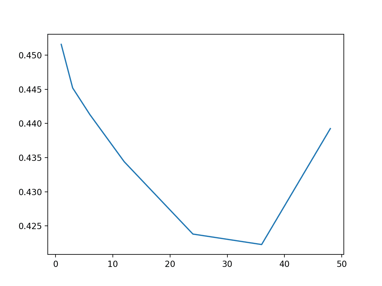
I experimented with the following number of lag observations:
1
[1, 3, 6, 12, 24, 36, 48]
The results were as follows:
1
2
3
4
5
6
7
1: 0.451
3: 0.445
6: 0.441
12: 0.434
24: 0.423
36: 0.422
48: 0.439
A plot of these results is provided below.
Line Plot of Number of Lag Observations vs MAE for Huber Regression
We can see a general trend of decreasing overall MAE with the increase in the number of lag observations, at least to a point after which error begins to rise again.
The results suggest, at least for the HuberRegressor algorithm, that 36 lag observations may be a good configuration achieving a MAE of 0.422.
Extensions
This section lists some ideas for extending the tutorial that you may wish to explore.
Data Preparation. Explore whether simple data preparation such as standardization or statistical outlier removal can improve model performance.
Engineered Features. Explore whether engineered features such as median value for forecasted hour of day can improve model performance
Meteorological Variables. Explore whether adding lag meteorological variables to the models can improve performance.
Cross-Site Models. Explore whether combining target variables of the same type and re-using the models across sites results in a performance improvement.
Algorithm Tuning. Explore whether tuning the hyperparameters of some of the better performing algorithms can result in performance improvements.
If you explore any of these extensions, I’d love to know.
Further Reading
This section provides more resources on the topic if you are looking to go deeper.
Will this example be also suitable for time dependent multivariate manufacturing data? In order to do prediction as well as root cause analysis for quality drop?
Great tutorial, Jason! I’ve learned some useful tricks, again. I’d be interested to know how long it takes for you to design, develop and test the code like this. This may useful for calculating some comparison metric for predicting the future level of data scientist in the specific lead times – another interesting time series forecasting problem 😉
It really depends on the experience of the developer. I wrote the code and words for this tutorial in less than one day, but I do have decades of experience.
if I want to predict after 1-hour air pollution but my dataset would not have chunkID, could I delete to_chucks and get_lead_times function but I don’t know the purpose of get_lead_time function .thx
Hi Jason,
IF i would like to predict aqhi after1 to 8 hours, what should i do?get_lead_times() is meaning for prediction hours but my dataset have not to chuck. What should i do on evaluate_forecasts()? I need to split row number of dataset for chunk id?? thx.
I’m having the same problem that Gary pointed out.
Though I have signed in to my Kaggle account, when I click the button to accept the rules, I remain stuck on the same page and no dataset is made available. Could this dataset no longer be downloadable? Could you please provide another link to it, if it exists?
Hello, doctor Jason! Your tutorial is so wonderful that I got a lot from it.
But, I have the same trouble that I cannot download the data. I am now in China, I can’t get the phone verification code. Can you show me another link about this?
To proceed, you must verify your
Kaggle account via your mobile phone.
After submitting your phone number, you’ll receive an SMS text message or a voice call for a code that you will enter on the next screen. You will only need to do this once. Do not use a public number or share your number with others.
Message and data rates may apply.
Terms and Conditions
Privacy Policy
Phone number (inc. country code)
+1-555-555-5555
Verifying with SMS
Switch to Voice
Thank you for your tutorials. I bought some of your books and what I’ve read so far they are all very useful for my current projects.
One of the one I’m working on right now is a multivariate multi-step time series classification forecasting problem.
i wonder what list of forcasting methods you would recommend for this kind of problems as you have mentioned for regression problems in this article.
Obviously we have to solve a non-linear problem.
but This is interesting as Huber regression, or robust regression with Huber loss, is a method that is designed to be robust to outliers in the training dataset.
The ML(EG .DL) is suit for handling the complex and nonlinear problems,but poor performance in this problem,
I noticed that the result was irrational.
How to discuss these results more deeply
I’ m a student and I just started learning ML.
I’ m following this tutorial to do practice and want to use LSTM model.
However, I have no idea about transfering the data shape of “supervised_train.npy” into three dimensional shape of LSTM.
Do I still need to fit a LSTM model for each variable and lead time combination?
Hi, Jason,
I had an interesting problem with my data to forecast using svr (using R) for stock market prediction. I found interesting things in that when i use svr or knn it works but output (test and correct) is delayed in graph. What will be the problem?? It means it is not predicting in advance. Any help!!!
Hi Jason and thanks again for your awesome ‘How to’s’!
I wonder if you have something on Multi-step forecasting on time series data with SVR, or if it even can be done?
Hi Jason, nice tutorial, thanks a lot! I have a question: when we want to do time series forecasting with mult-variate-timeseries, do the several input metrics have to be previously checked separately positively for correlating to the target feature (e.g. Pearson correlation factor >0.5)? Thanks in advance!
I am concerned right now about implementing a predictive model for multiple Ys and multiple Xs.
The dataset corresponds to these variables across several countries of the world and 17 years of data (1 year per row)
So far, I have imputated missing data, ran correlation analysis across the variables and designed a random forest regressor in Python.
I am struggling on the interpretation part of the random forest. I assigned all the Xs and all the Ys to the regressor and I am not sure about how to go on to interpret the results.
Upon running the linear algorithm for the dataset i have, i encountered an error but im unsure on how to fix it. The error:
Traceback (most recent call last):
File “compare.py”, line 183, in
evaluate_models(models, train, test, actual)
File “compare.py”, line 164, in evaluate_models
fits = fit_models(model, train)
File “compare.py”, line 59, in fit_models
X, y = data[:, :-1], data[:,-1]
IndexError: too many indices for array
the results of print train and test shape is:
((96, 3), (160, 96, 3))
I’m interested in exploring the Cross-Site Modeling of the problem as I’m working on a similar problem.
Let’s assume we have 10 target variables, and each variable per site. Do you think it’s possible to combine the target variables to form one dataset across all sites upon which we can fit a single model for all the sites? Thus, we can use the said model to forecast each lead time based on direct strategy – depending on the forecast horizons, we can have multiple models based on that single model.
If the said approach is possible, should we just overlook any duplicate on the date-time index as a result of combining the variables from different sites?
The changes in the imdb.py did not work for me (likely multiple environment issues) – but the code update below did:
current:
train = load(‘AirQualityPrediction/supervised_train.npy’)
test = load(‘AirQualityPrediction/supervised_test.npy’)
update to:
train = load(‘AirQualityPrediction/supervised_train.npy’, allow_pickle=True)
test = load(‘AirQualityPrediction/supervised_test.npy’, allow_pickle=True)
-GM
thank you for all the great product and tutorials here.
Hi Jason,
This is great. I did some work on bayesian localized conditional autoregressive (LCAR) forecasting model on R. Still struggling to conclude. I would love your help on an R tutorial on Bayesian LCAR and similarly on python.
Hello, Dr.Jason.
Could you make a recursive LSTM example?
I mean, If we want to predict t+2 or t+3, we could use t+1 model output.
I want to know how can we use output as input.
One question, i need to ask. How do you evaluate that your model is overfitted. I see that you calculate MAE over test data. How do you know if a MAE of almost zero is a signal of overfitting or you are doing a very good job.
Thank you. I’d like to ask you how to consider the order of multiple variables in the multi-step and multi variable situation. For example, a production process in a factory has three machines, each with the characteristics of temperature (T) and speed (s), T1, S1 – > T2, S2->T3, S3. How to consider the order?
“A single model is developed to make one-step forecasts, and the model is used recursively where prior forecasts are used as input to forecast the subsequent lead time.”
Thank you very much. Could we also use recursive method to predict when Multivariate-data are not Univariate-data?
Thank you very much. I tried to explain my question. As you mentioned in this article(https://machinelearningmastery.com/multivariate-time-series-forecasting-lstms-keras/), we can see the 8 input variables (input series) and the 1 output variable. If we use the recursive multi step forecast method to predict the next two days temperature, as below
But we don’t have Var2 (t), Var3 (t), Var4 (t), Var5 (t), Var6 (t), Var7 (t), Var8 (t) these input parameters at present. Do we need to predict them separately?
You could try predicting them.
You could try padding with zeros.
You could try persisting the last values.
You could try using a direct method instead.
Hi Jason, its possible to do forecasting of time series with multiple time series? For example if you have many flights with diferent time series? And if you have some example of somthing similar!
HI json i have data set like staion 1 station 2 station 3 temperature so i need to forecast all the three station respectively , but these are not correlated , all three are separate stations so my question is can we forecast all the three station in one single model ? or we need to build separate model ?
Apologies for dumb question. Not sure if i’m doing something wrong but i’m having a hard time finding the input data to follow along. The site says: An error occurred: Data not found
I reported it but no reply from Kaggle Support :(. Would it be possible for you to upload it to kaggle datasets or google drive and share the link with us?
I am using RandomForestRegressor from sklearn. I used it for univariate time series and it was good. Now, I am struggling with multivariate. Could you help me if there is a tutorial about it, please?
my train_x.shape: (205, 7, 18) train_y.shape: (205, 1)
I am struggling with the data shape as I got :
ValueError: Found array with dim 3. Estimator expected <= 2.
That was a very detailed tutorial and helps a lot.
I have a confusion, and will appreciated if it’s answered
suppose that we’ve been given historical data to forecast.
we’ve two options:
1- an automated open-source time-series forecasting tool (free of cost)
we feed-in the data and get the forecast
2- develop our own machine learning model to do the same.
I am confused, that if option#1 is available, then what edge should option#2 has over option#1 that we go for it.
Or may be the automated tools lack some capabilities, like feature-engineering differ case by case, and it is not generic, and if we need to take maximum advantage from these tools we anyway have to do our own feature engineering before we feed in the data into them.
I’m having difficulty accessing the dataset from kaggle. As some else suggested, I verified my account on my phone but not luck. I even installed the kaggle-api, created a token and but I get a 403 when trying to access it from the command line. Any one else having this issue?
Thank you for this tutorial. I am a beginner in ML and don’t understand a statement made in this tutorial. You stated:
“When working with the naive models, we are only interested in the target variables, and none of the input meteorological variables. Therefore, we can remove the input data and have the train and test data only comprised of the 39 target variables for each chunk, as well as the position within chunk and hour of observation.”
I don’t understand this, as surely when trying to predict the pollution at any point, some meteorological data like Wind Direction or such would be relevant here. If you could direct me to a link where this is explained in more detail it would be much appreciated.
Hi Jason, your books and blog has been a real help so far. A big thanks. Regarding this tutorial, the dataset is not available in kaggle. Anywhere else it might be available, you might be aware of ?
your books and blogs are awesome! They have been a great help so far.
I try to find a tutorial or tips for developing a multivariate time series classification model.
My data look similar to the one processed here (medical data), but I want to predict a binary outcome.
E.g. having different patients with 50 variables, each measured at a different time -> 50 time series per patient. And I want to predict if the patient has/develops) a specific disease.
I am struggling with the correct data preparation. How should the input look like and would be a LSTM a good choice?
Thank you very much
Develop Multivariate Multi-Step Time Series Forecasting Models
Thanks a lot for sharing these and other LSTM-time series articles. My question is pertaining to the data normalization. I have seen you taking two approaches, first is dividing the data into train and test and then fitting the train dataset to the scaler and transforming the test. The other is first normalizing the entire dataset and then dividing into train and test. My question is which is a better approach. For some context, I will be creating a transform this using the create_dataset() function and a lookback of 30.
i have a dataset where the target variable have data something like as below:
E_Codes
0
0
0
40
0
0
0
90
0
0
0
10
0
0
these are actually the error codes generated by a machine at the production line, the goal is to predict that when would in the next ‘n’ cycles we will have a specific error code. I have seen many examples of forecasting using LSTM but all are predicting the continuous values such as Price, weather or stocks etch.
this problem is a kind of classification but needs forecasting instead of simple classification
would you please let me know which tutorial should I follow? how should I phrase my question to google problems related to this kind of data?
Hi Jason, great tutorial. Maybe a stupid question, but why was the Kaggle winner’s MAE so much lower than the random forest regressor that you evaluated?
Thank you for this tutorial, I have a question about the chunks. Do they improve the precision of the result or something … can we do the same approach on a dataset that isn’t grouped by chunks
Thank you for your detail tutorial. How will the tutorial change if my data have different chunks but only one target variable?
I think some people above have 3D array instead of 2D array. I have the same problem. My train and test shape are:
train_data shape is (1, 10) in which 1 is number of target variable, 10 is leads_time
test_data shape is (288, 1, 12) in which 288 is number of chunks, 1 is number of target variable, 12 is n_lag?
My test_data shape is 3D array while train_data shape seems too be correct.
This is great article. But I didn’t see any article/paper talking about the traditional time series test such as stationarity in the context of machine learning methods. When I ensemble different time series and assign a weightage to get the final prediction, do I have to check on the stationarity of the time series model such as SARIMA, ARIMA etc? Or as the machine learning can be self adaptive and does that mean it will evolve to even predict with non-stationary data like optimize the P, D, Q so that I don’t have to worry about its stationarity?
It is really a fantastic tutorial. Many things to understand. while I am in middle of developing the similar model, I just wanted to know why have you here used forward-fill and backward-fill both for interpolating the NaN hours? Wouldn’t the forward-fill will suffice for our task?
Assume for series x[0], x[1], …, x[n] and you get only odd-numbered data. Then forward fill help use set x[2]=x[1], x[4]=x[3], etc. But then x[0] is still NaN unless you backfill it with x[1]
Thank you for the very helpful tutorial! Quick question: supervised machine learning can use whatever time points set to learn, eg day 1,2,5 to predict day 6. Can a classical model such as ARIMA etc. do the same, taking non-contiguous time series as input, or must it take contiguous series day 1,2,3,4,5 to forecast day 6?
This means that the interval between the observations is not consistent, but may vary.
You can learn more about contiguous vs discontiguous time series datasets in this post:
Taxonomy of Time Series Forecasting Problems
There are many ways to handle data in this form and you must discover the approach that works well or best for your specific dataset and chosen model.
The most common approach is to frame the discontiguous time series as contiguous and the observations for the newly observation times as missing (e.g. a contiguous time series with missing values).
Some ideas you may want to explore include:
Ignore the discontiguous nature of the problem and model the data as-is.
Resample the data (e.g. upsample) to have a consistent interval between observations.
Impute the observations to form a consistent interval.
Pad the observations for form a consistent interval and use a Masking layer to ignore the padded values.
Hi, Jason. I may have some doubts about using linear regression methods applied to this dataset. I am new to machine learning and could you take some time to help me? Thank you very much!
First of all, applying what I have learned in class, on this dataset, I think it is important to create a model like “variable1~variable2+variable3+… +variable11+Time”. But I have read your explanation of the code, are you using only univariate lags as predictions? Something like “variable1(t)~variable1(t-1)+variable1(t-2)”. I’m not sure if I understand this correctly, but here I’m a bit confused as to why linear regression doesn’t take into account the linear relationship between the 12 variables. I look forward to your reply, thank you very much!
Sorry, I’m not modeling this data set, I’m just learning your code. But I wonder why the linear relationship between the 12 variables is not taken into account when establishing the linear model. The model only considers the hysteresis of each single variable.
Thank you for the effort you put in writing this beneficial post.
Is it possible to make some manipulation to one of the series in the multivariate time series before making forecast with the aim of expecting the modification to be propagated in the result of the forecast?
Once again, thank you!
Thank you for the great content, i really learned a lot.
i have a question please. is it possible to do time series forecasting for air pollution on multiple sites if the locations in the dataset are all in 1 column?
Also in the dataset provided, where are the locations? is each feature repeated on multiple columns meaning one for each location? but i don’t see the locations given in the dataset.
Hi Nourhan…Each location would have its own dataset. The columns of each would represent each feature and the rows would represent time. This means that each column would represent a separate time-series.
When i run the first part of the code, the data_prep function produces the following error:
return array(train_data), array(test_data)
ValueError: setting an array element with a sequence. The requested array has an inhomogeneous shape after 2 dimensions. The detected shape was (39, 10) + inhomogeneous part.
It seems like the train_data and test_data lists don´t have a consistent shape.
ValueError: setting an array element with a sequence. The requested array has an inhomogeneous shape after 1 dimensions. The detected shape was (207,) + inhomogeneous part.
I am getting errors with code that I copied and pasted:
“—————————————————————————
ValueError Traceback (most recent call last)
Cell In[113], line 163
161 # convert training data into supervised learning data
162 n_lag = 12
–> 163 train_data, test_data = data_prep(train_chunks, n_lag)
164 print(train_data.shape, test_data.shape)
165 # save train and test sets to file
Cell In[113], line 153, in data_prep(chunks, n_lag, n_vars)
151 for lead_time in range(len(lead_times)):
152 train_data[var][lead_time] = array(train_data[var][lead_time])
–> 153 return array(train_data), array(test_data)
ValueError: setting an array element with a sequence. The requested array has an inhomogeneous shape after 2 dimensions. The detected shape was (39, 10) + inhomogeneous part.”


Wow, that’s a complete tutorial! Tnks
Thanks!
Will this example be also suitable for time dependent multivariate manufacturing data? In order to do prediction as well as root cause analysis for quality drop?
Perhaps try it and compare the results to other methods?
i d like to apply something similar to the lottery viewed as time series with multiple time steps
You cannot predict the lottery:
https://machinelearningmastery.com/faq/single-faq/can-i-use-machine-learning-to-predict-the-lottery
Great tutorial, Jason! I’ve learned some useful tricks, again. I’d be interested to know how long it takes for you to design, develop and test the code like this. This may useful for calculating some comparison metric for predicting the future level of data scientist in the specific lead times – another interesting time series forecasting problem 😉
It really depends on the experience of the developer. I wrote the code and words for this tutorial in less than one day, but I do have decades of experience.
That’s impressive! This is clearly the “ML guru” level.
Thanks.
Exactly i_i
Guru level.
Thanks for publishing a such complete tutorial.
Very useful. Couldn’t swallow all code at once, will have to work on that.
Will definitely be useful.
Really fantastic work Jason… Please Provide your valuable suggestion and guide me how to implement in JAVA…
Sorry, Id on’t have examples in Java.
if I want to predict after 1-hour air pollution but my dataset would not have chunkID, could I delete to_chucks and get_lead_times function but I don’t know the purpose of get_lead_time function .thx
This is a complex example, perhaps start with something simpler like the electricity usage forecasting:
https://machinelearningmastery.com/start-here/#deep_learning_time_series
Hi Jason,
IF i would like to predict aqhi after1 to 8 hours, what should i do?get_lead_times() is meaning for prediction hours but my dataset have not to chuck. What should i do on evaluate_forecasts()? I need to split row number of dataset for chunk id?? thx.
I would recommend following this tutorial instead:
https://machinelearningmastery.com/multi-step-time-series-forecasting-with-machine-learning-models-for-household-electricity-consumption/
can’t get the air quality dataset. when i clicked the accept rules button, the page refreshed…
You must sign-in to Kaggle and then click the “download all” button.
I’m having the same problem that Gary pointed out.
Though I have signed in to my Kaggle account, when I click the button to accept the rules, I remain stuck on the same page and no dataset is made available. Could this dataset no longer be downloadable? Could you please provide another link to it, if it exists?
Try refreshing this URL after logging in:
https://www.kaggle.com/c/dsg-hackathon/data
Note the “Download All” button.
even after signing in Kaggle account unable to download data. could you please provide another link
I’m sorry to heat that, what is the problem exactly?
Hello, doctor Jason! Your tutorial is so wonderful that I got a lot from it.
But, I have the same trouble that I cannot download the data. I am now in China, I can’t get the phone verification code. Can you show me another link about this?
Sorry to hear that. I don’t think a phone code is required, I’m suprised.
To proceed, you must verify your
Kaggle account via your mobile phone.
After submitting your phone number, you’ll receive an SMS text message or a voice call for a code that you will enter on the next screen. You will only need to do this once. Do not use a public number or share your number with others.
Message and data rates may apply.
Terms and Conditions
Privacy Policy
Phone number (inc. country code)
+1-555-555-5555
Verifying with SMS
Switch to Voice
Wow, I have never seen this. It must be new! Sorry to hear that.
Hello. Yes you do require a phone number to download kaggle data with a new account 🙂
If it doesn’t work, just contact kaggle.
Wow, that is crazy!
That never used to be the case, perhaps it is a new thing since google acquired the company.
Hi Jason,
Thank you for your tutorials. I bought some of your books and what I’ve read so far they are all very useful for my current projects.
One of the one I’m working on right now is a multivariate multi-step time series classification forecasting problem.
i wonder what list of forcasting methods you would recommend for this kind of problems as you have mentioned for regression problems in this article.
Thank you in advance.
Perhaps try modeling each output with a direct model as a baseline for comparison.
So nice to find an other tutorial for that dataset! Thank you Jason!
Would an LSTM model be proper for forecasting for that dataset?
There is no idea of “proper”, only some models that perform well and some that do not.
Obviously we have to solve a non-linear problem.
but This is interesting as Huber regression, or robust regression with Huber loss, is a method that is designed to be robust to outliers in the training dataset.
The ML(EG .DL) is suit for handling the complex and nonlinear problems,but poor performance in this problem,
I noticed that the result was irrational.
How to discuss these results more deeply
Sorry, Id on’t follow your question, what do you mean discuss more deeply?
Do you mean how to analyze results? If so, in what way?
I learned alot from this post!
Thanks for sharing
Thanks, I’m glad it was helpful.
Hi Jason,
Good Morning,
Can you please let us know when to use which time series algorithm? Like when to use ARIMA? When to use LSTM ?
Could you please let us know the implementation for multivariate time series implementation using ARIMA in Python.
Thanks
Yes, I recommend this process:
https://machinelearningmastery.com/how-to-develop-a-skilful-time-series-forecasting-model/
Thanks Jason,
Is it possible to implement multivariate time series using ARIMA in Python. Could you please share if you have such tutorials.
Thanks
Yes, it would be VAR or VARIMA. This might help as a start:
https://machinelearningmastery.com/time-series-forecasting-methods-in-python-cheat-sheet/
Thank You so much!!!
I’m glad it helped.
Is there a tutorial on Stochastic Forest processing time series?
I’ve not heard of that method, sorry.
Hi,Jason. Thank you for your tutorial!
I’ m a student and I just started learning ML.
I’ m following this tutorial to do practice and want to use LSTM model.
However, I have no idea about transfering the data shape of “supervised_train.npy” into three dimensional shape of LSTM.
Do I still need to fit a LSTM model for each variable and lead time combination?
Thanks!! QAQ
Great question, I believe this will help:
https://machinelearningmastery.com/faq/single-faq/how-do-i-prepare-my-data-for-an-lstm
Hi, Jason,
I had an interesting problem with my data to forecast using svr (using R) for stock market prediction. I found interesting things in that when i use svr or knn it works but output (test and correct) is delayed in graph. What will be the problem?? It means it is not predicting in advance. Any help!!!
The stock market is not predictable, that will be the main problem:
https://machinelearningmastery.com/faq/single-faq/can-you-help-me-with-machine-learning-for-finance-or-the-stock-market
Hi Jason and thanks again for your awesome ‘How to’s’!
I wonder if you have something on Multi-step forecasting on time series data with SVR, or if it even can be done?
Thank you!
Yes, you could use a direct strategy:
https://machinelearningmastery.com/multi-step-time-series-forecasting/
There is an example here I believe:
https://machinelearningmastery.com/multi-step-time-series-forecasting-with-machine-learning-models-for-household-electricity-consumption/
Awesome tutorial.. Thank you
Thanks, I’m glad it helped!
Hi Jason, nice tutorial, thanks a lot! I have a question: when we want to do time series forecasting with mult-variate-timeseries, do the several input metrics have to be previously checked separately positively for correlating to the target feature (e.g. Pearson correlation factor >0.5)? Thanks in advance!
Perhaps. It could be misleading if the outcome is a nonlinear combination of inputs.
I generally recommend fitting models with all/most data and lear the ensemble/model discover what features work best.
Jason, fantastic tutorial.
I am concerned right now about implementing a predictive model for multiple Ys and multiple Xs.
The dataset corresponds to these variables across several countries of the world and 17 years of data (1 year per row)
So far, I have imputated missing data, ran correlation analysis across the variables and designed a random forest regressor in Python.
I am struggling on the interpretation part of the random forest. I assigned all the Xs and all the Ys to the regressor and I am not sure about how to go on to interpret the results.
Perhaps you can use the error of the model on predictions to interpret the skill of the model?
Is that what you mean?
Hi Jason,
Upon running the linear algorithm for the dataset i have, i encountered an error but im unsure on how to fix it. The error:
Traceback (most recent call last):
File “compare.py”, line 183, in
evaluate_models(models, train, test, actual)
File “compare.py”, line 164, in evaluate_models
fits = fit_models(model, train)
File “compare.py”, line 59, in fit_models
X, y = data[:, :-1], data[:,-1]
IndexError: too many indices for array
the results of print train and test shape is:
((96, 3), (160, 96, 3))
Perhaps confirm that the loaded data meets the expectation of the code, work with a single sample first and step through each line.
I get the same issue:
the results of print train and test shape is:
((6, 3), (20, 6, 3))
I’ve tried many different things.
I looked at your dataset and adjusted everything, I still get 2D,3D instead of 2D,2D like you do.
Sorry to hear that. I have some suggestions here that may help:
https://machinelearningmastery.com/faq/single-faq/can-you-read-review-or-debug-my-code
Hi Dr. Jason,
I’m interested in exploring the Cross-Site Modeling of the problem as I’m working on a similar problem.
Let’s assume we have 10 target variables, and each variable per site. Do you think it’s possible to combine the target variables to form one dataset across all sites upon which we can fit a single model for all the sites? Thus, we can use the said model to forecast each lead time based on direct strategy – depending on the forecast horizons, we can have multiple models based on that single model.
If the said approach is possible, should we just overlook any duplicate on the date-time index as a result of combining the variables from different sites?
Thanks in advance
Yes, I have some suggestions here:
https://machinelearningmastery.com/faq/single-faq/how-to-develop-forecast-models-for-multiple-sites
Those approaches you listed very relevant. I think a transfer learning strategy will play a vital role in exploring the said problem, isn’t it?
Perhaps try it and see?
Thanks
With the most recent version of numpy:1.16.3 the following lines are generating a documented error:
value error:’Object arrays cannot be loaded when allow_pickle=False’
documentation: https://stackoverflow.com/questions/55890813/how-to-fix-object-arrays-cannot-be-loaded-when-allow-pickle-false-for-imdb-loa
and
https://github.com/tensorflow/tensorflow/commit/79a8d5cdad942b9853aa70b59441983b42a8aeb3#diff-b0a029ad68170f59173eb2f6660cd8e0
The changes in the imdb.py did not work for me (likely multiple environment issues) – but the code update below did:
current:
train = load(‘AirQualityPrediction/supervised_train.npy’)
test = load(‘AirQualityPrediction/supervised_test.npy’)
update to:
train = load(‘AirQualityPrediction/supervised_train.npy’, allow_pickle=True)
test = load(‘AirQualityPrediction/supervised_test.npy’, allow_pickle=True)
-GM
thank you for all the great product and tutorials here.
Thanks, I have updated the example to fix the bug with the new version of NumPy.
can you please write the same tutorial for electricity dataset, the multi step tutorial from https://machinelearningmastery.com/multi-step-time-series-forecasting-with-machine-learning-models-for-household-electricity-consumption/ for electricity data is essentially a univariate forecasting. Can you improve this using all the variables of the electricity data and have machine learning models.
Thanks for the suggestion.
Hi Jason,
This is great. I did some work on bayesian localized conditional autoregressive (LCAR) forecasting model on R. Still struggling to conclude. I would love your help on an R tutorial on Bayesian LCAR and similarly on python.
Many thanks in advance.
Thanks for the suggestion!
Hello, Dr.Jason.
Could you make a recursive LSTM example?
I mean, If we want to predict t+2 or t+3, we could use t+1 model output.
I want to know how can we use output as input.
Thanks.
Thanks for the suggestion.
Hi Jason, great article.
One question, i need to ask. How do you evaluate that your model is overfitted. I see that you calculate MAE over test data. How do you know if a MAE of almost zero is a signal of overfitting or you are doing a very good job.
Thanks in advance.
Good question, see this tutorial:
https://machinelearningmastery.com/learning-curves-for-diagnosing-machine-learning-model-performance/
See solutions here:
https://machinelearningmastery.com/introduction-to-regularization-to-reduce-overfitting-and-improve-generalization-error/
Dear Sir
very much thankful to you, let me know RNN-LSTM code to predict air pollution(forecasting)
You’re welcome.
Thank you. I’d like to ask you how to consider the order of multiple variables in the multi-step and multi variable situation. For example, a production process in a factory has three machines, each with the characteristics of temperature (T) and speed (s), T1, S1 – > T2, S2->T3, S3. How to consider the order?
Order of features to the LSTM does not seem to matter.
“A single model is developed to make one-step forecasts, and the model is used recursively where prior forecasts are used as input to forecast the subsequent lead time.”
Thank you very much. Could we also use recursive method to predict when Multivariate-data are not Univariate-data?
Yes, see this:
https://machinelearningmastery.com/multi-step-time-series-forecasting/
Thank you. but I mean if I use multiple variables (multiple features) to predict, how do I use recursive method?
In the same way as one feature.
Perhaps I don’t understand the problem you’re having?
Thank you very much. I tried to explain my question. As you mentioned in this article(https://machinelearningmastery.com/multivariate-time-series-forecasting-lstms-keras/), we can see the 8 input variables (input series) and the 1 output variable. If we use the recursive multi step forecast method to predict the next two days temperature, as below
Var1(t)= model(Var1(t-1),Var2(t-1),Var3(t-1),Var4(t-1),Var5(t-1),Var6(t-1),Var7 (t-1),Var8(t-1))
Var1(t+1)= model(Var1(t),Var2(t),Var3(t),Var4(t),Var5(t),Var6(t),Var7(t),Var8(t))
But we don’t have Var2 (t), Var3 (t), Var4 (t), Var5 (t), Var6 (t), Var7 (t), Var8 (t) these input parameters at present. Do we need to predict them separately?
Ah I see, good question.
You could try predicting them.
You could try padding with zeros.
You could try persisting the last values.
You could try using a direct method instead.
I’ll try. Thank you very much
Hi Jason, its possible to do forecasting of time series with multiple time series? For example if you have many flights with diferent time series? And if you have some example of somthing similar!
Thank you!
Yes, see a good introductory example in this tutorial:
https://machinelearningmastery.com/how-to-develop-lstm-models-for-time-series-forecasting/
HI json i have data set like staion 1 station 2 station 3 temperature so i need to forecast all the three station respectively , but these are not correlated , all three are separate stations so my question is can we forecast all the three station in one single model ? or we need to build separate model ?
Great question, this will give you ideas:
https://machinelearningmastery.com/faq/single-faq/how-to-develop-forecast-models-for-multiple-sites
Apologies for dumb question. Not sure if i’m doing something wrong but i’m having a hard time finding the input data to follow along. The site says: An error occurred: Data not found
https://www.kaggle.com/c/dsg-hackathon/data
Agreed, looks like kaggle is currently broken.
Hi Jason, do you have a copy of the dataset? I’m getting a “data not available” error on Kaggle
I do, but it is very large.
Perhaps report the fault to kaggle.
I reported it but no reply from Kaggle Support :(. Would it be possible for you to upload it to kaggle datasets or google drive and share the link with us?
Not sure I can do that, sorry.
This was the response from the kaggle team:
At the request of that competition’s host, we no longer offer data for that competition. Consider trying another competition instead: https://www.kaggle.com/competitions or an open dataset: https://www.kaggle.com/datasets. Or, post a request on our dataset forum: https://www.kaggle.com/data.
Oh dear.
created this thread in kaggle about the missing dataset: https://www.kaggle.com/data/154202
Nice!
you might want to change your download link to :
https://archive.ics.uci.edu/ml/datasets/Air+Quality
sorry Jason, that dataset isn’t what we’re looking for, nevermind 🙁
No problem.
Is that the same dataset?
Hello, Dr.Jason!
Except LSTM and CNN, what about reinforcement learning for time series forecasting?
I don’t have experience with RL for time series forecasting, sorry. Does not sound like a good fit for the techniques.
Hello Doctor,
We are not getting the dataset for this model. Please try to arrange it.
Perhaps move on to another tutorial:
https://machinelearningmastery.com/start-here/#deep_learning_time_series
Hi Jason,
I am using RandomForestRegressor from sklearn. I used it for univariate time series and it was good. Now, I am struggling with multivariate. Could you help me if there is a tutorial about it, please?
my train_x.shape: (205, 7, 18) train_y.shape: (205, 1)
I am struggling with the data shape as I got :
ValueError: Found array with dim 3. Estimator expected <= 2.
Any help please?
Thanks in Advance,
Perhaps this will help:
https://machinelearningmastery.com/multi-output-regression-models-with-python/
That was a very detailed tutorial and helps a lot.
I have a confusion, and will appreciated if it’s answered
suppose that we’ve been given historical data to forecast.
we’ve two options:
1- an automated open-source time-series forecasting tool (free of cost)
we feed-in the data and get the forecast
2- develop our own machine learning model to do the same.
I am confused, that if option#1 is available, then what edge should option#2 has over option#1 that we go for it.
Or may be the automated tools lack some capabilities, like feature-engineering differ case by case, and it is not generic, and if we need to take maximum advantage from these tools we anyway have to do our own feature engineering before we feed in the data into them.
your response is much appreciated
I’m not aware of automated tools, sorry.
I’m having difficulty accessing the dataset from kaggle. As some else suggested, I verified my account on my phone but not luck. I even installed the kaggle-api, created a token and but I get a 403 when trying to access it from the command line. Any one else having this issue?
It appears that may have taken the dataset down. Which is a real shame.
Try contacting their support.
Thank you for this tutorial. I am a beginner in ML and don’t understand a statement made in this tutorial. You stated:
“When working with the naive models, we are only interested in the target variables, and none of the input meteorological variables. Therefore, we can remove the input data and have the train and test data only comprised of the 39 target variables for each chunk, as well as the position within chunk and hour of observation.”
I don’t understand this, as surely when trying to predict the pollution at any point, some meteorological data like Wind Direction or such would be relevant here. If you could direct me to a link where this is explained in more detail it would be much appreciated.
You’re welcome.
It is a simplification of the problem for the tutorial. You can frame the problem anyway you like, I encourage it!
Hi Jason, your books and blog has been a real help so far. A big thanks. Regarding this tutorial, the dataset is not available in kaggle. Anywhere else it might be available, you might be aware of ?
Thanks!
Perhaps contact kaggle to see if they will release it again?
Perhaps try an alternate dataset?
Perhaps try an alternate tutorial?
Hi Jason, Can I get an idea about which NN model should be use to multivariate weather prediction using Temperature, humidity, pressure etc.
Good question, see this:
https://machinelearningmastery.com/faq/single-faq/what-algorithm-config-should-i-use
And this:
https://machinelearningmastery.com/how-to-develop-a-skilful-time-series-forecasting-model/
Thank you very much for the quick reply
You’re welcome.
Hello Jason,
your books and blogs are awesome! They have been a great help so far.
I try to find a tutorial or tips for developing a multivariate time series classification model.
My data look similar to the one processed here (medical data), but I want to predict a binary outcome.
E.g. having different patients with 50 variables, each measured at a different time -> 50 time series per patient. And I want to predict if the patient has/develops) a specific disease.
I am struggling with the correct data preparation. How should the input look like and would be a LSTM a good choice?
Thank you very much
Develop Multivariate Multi-Step Time Series Forecasting Models
Thanks!
Sounds like time series classification. I recommend comparing MLP, CNN, LSTM, ML and linear models and discover what works best for your dataset.
Thank you very much for your advice.
Would these models also work well with only small time series, with 2-3 time stamps?
Probably not.
Hi Jason,
Thanks a lot for sharing these and other LSTM-time series articles. My question is pertaining to the data normalization. I have seen you taking two approaches, first is dividing the data into train and test and then fitting the train dataset to the scaler and transforming the test. The other is first normalizing the entire dataset and then dividing into train and test. My question is which is a better approach. For some context, I will be creating a transform this using the create_dataset() function and a lookback of 30.
The former approach is generally appropriate. The latter is lazy and only used in tutorials.
Hello Jason,
i have a dataset where the target variable have data something like as below:
E_Codes
0
0
0
40
0
0
0
90
0
0
0
10
0
0
these are actually the error codes generated by a machine at the production line, the goal is to predict that when would in the next ‘n’ cycles we will have a specific error code. I have seen many examples of forecasting using LSTM but all are predicting the continuous values such as Price, weather or stocks etch.
this problem is a kind of classification but needs forecasting instead of simple classification
would you please let me know which tutorial should I follow? how should I phrase my question to google problems related to this kind of data?
You can see examples of time series forecasting with deep learning models here:
https://machinelearningmastery.com/start-here/#deep_learning_time_series
Hi Jason, great tutorial. Maybe a stupid question, but why was the Kaggle winner’s MAE so much lower than the random forest regressor that you evaluated?
Thanks.
I did not optimize the model, just demonstrated how to develop a model for the dataset and framing of the problem.
Thank you for this tutorial, I have a question about the chunks. Do they improve the precision of the result or something … can we do the same approach on a dataset that isn’t grouped by chunks
You’re welcome.
Yes, it is just an artefact of how this specific dataset was prepared and made available. You can prepare data any way you like, perhaps start here:
https://machinelearningmastery.com/start-here/#deep_learning_time_series
Hi Dr.Brownlee,
Thank you for your detail tutorial. How will the tutorial change if my data have different chunks but only one target variable?
I think some people above have 3D array instead of 2D array. I have the same problem. My train and test shape are:
train_data shape is (1, 10) in which 1 is number of target variable, 10 is leads_time
test_data shape is (288, 1, 12) in which 288 is number of chunks, 1 is number of target variable, 12 is n_lag?
My test_data shape is 3D array while train_data shape seems too be correct.
Perhaps this will help:
https://machinelearningmastery.com/faq/single-faq/what-is-the-difference-between-samples-timesteps-and-features-for-lstm-input
Hi Jason,
This is great article. But I didn’t see any article/paper talking about the traditional time series test such as stationarity in the context of machine learning methods. When I ensemble different time series and assign a weightage to get the final prediction, do I have to check on the stationarity of the time series model such as SARIMA, ARIMA etc? Or as the machine learning can be self adaptive and does that mean it will evolve to even predict with non-stationary data like optimize the P, D, Q so that I don’t have to worry about its stationarity?
Appreciate your thoughts on this.
Thank you.
It depends on the data and the model. Most models will work better if you make the series stationary first.
Hi Jason,
It is really a fantastic tutorial. Many things to understand. while I am in middle of developing the similar model, I just wanted to know why have you here used forward-fill and backward-fill both for interpolating the NaN hours? Wouldn’t the forward-fill will suffice for our task?
Thanks in advance!
Assume for series x[0], x[1], …, x[n] and you get only odd-numbered data. Then forward fill help use set x[2]=x[1], x[4]=x[3], etc. But then x[0] is still NaN unless you backfill it with x[1]
yes, I discovered it. Thanks for clarification !!
chunk_ids = unique(values[:, 1])
Your tutorial doesn’t work even from first command. what is values dataframe we didn’t define anything like that
Hi Enes,
Did you use the complete code listings in the tutorial?
Regards,
Thank you for the very helpful tutorial! Quick question: supervised machine learning can use whatever time points set to learn, eg day 1,2,5 to predict day 6. Can a classical model such as ARIMA etc. do the same, taking non-contiguous time series as input, or must it take contiguous series day 1,2,3,4,5 to forecast day 6?
Hi Le…Some time series data is discontiguous.
This means that the interval between the observations is not consistent, but may vary.
You can learn more about contiguous vs discontiguous time series datasets in this post:
Taxonomy of Time Series Forecasting Problems
There are many ways to handle data in this form and you must discover the approach that works well or best for your specific dataset and chosen model.
The most common approach is to frame the discontiguous time series as contiguous and the observations for the newly observation times as missing (e.g. a contiguous time series with missing values).
Some ideas you may want to explore include:
Ignore the discontiguous nature of the problem and model the data as-is.
Resample the data (e.g. upsample) to have a consistent interval between observations.
Impute the observations to form a consistent interval.
Pad the observations for form a consistent interval and use a Masking layer to ignore the padded values.
Hi, Jason. I may have some doubts about using linear regression methods applied to this dataset. I am new to machine learning and could you take some time to help me? Thank you very much!
First of all, applying what I have learned in class, on this dataset, I think it is important to create a model like “variable1~variable2+variable3+… +variable11+Time”. But I have read your explanation of the code, are you using only univariate lags as predictions? Something like “variable1(t)~variable1(t-1)+variable1(t-2)”. I’m not sure if I understand this correctly, but here I’m a bit confused as to why linear regression doesn’t take into account the linear relationship between the 12 variables. I look forward to your reply, thank you very much!
Hi YIZE…Have you built a model for this dataset? If so, please let us know your findings.
Sorry, I’m not modeling this data set, I’m just learning your code. But I wonder why the linear relationship between the 12 variables is not taken into account when establishing the linear model. The model only considers the hysteresis of each single variable.
Hi Jason,
Thank you for the effort you put in writing this beneficial post.
Is it possible to make some manipulation to one of the series in the multivariate time series before making forecast with the aim of expecting the modification to be propagated in the result of the forecast?
Once again, thank you!
Hi Dr Jason,
Thank you for the great content, i really learned a lot.
i have a question please. is it possible to do time series forecasting for air pollution on multiple sites if the locations in the dataset are all in 1 column?
Also in the dataset provided, where are the locations? is each feature repeated on multiple columns meaning one for each location? but i don’t see the locations given in the dataset.
Thank you a lot for your help.
Hi Nourhan…Each location would have its own dataset. The columns of each would represent each feature and the rows would represent time. This means that each column would represent a separate time-series.
Hi Jason,
When i run the first part of the code, the data_prep function produces the following error:
return array(train_data), array(test_data)
ValueError: setting an array element with a sequence. The requested array has an inhomogeneous shape after 2 dimensions. The detected shape was (39, 10) + inhomogeneous part.
It seems like the train_data and test_data lists don´t have a consistent shape.
Thanks
Hi Felix…Did you copy and paste code or type it in? Also, the following discussions may be of interest to you:
https://stackoverflow.com/questions/4674473/valueerror-setting-an-array-element-with-a-sequence
https://www.geeksforgeeks.org/how-to-fix-valueerror-setting-an-array-element-with-a-sequence/
I copied the code exactly as it is.
The problem is the variable train_chunks:
print(array(train_chunks).shape)
ValueError: setting an array element with a sequence. The requested array has an inhomogeneous shape after 1 dimensions. The detected shape was (207,) + inhomogeneous part.
I am getting errors with code that I copied and pasted:
“—————————————————————————
ValueError Traceback (most recent call last)
Cell In[113], line 163
161 # convert training data into supervised learning data
162 n_lag = 12
–> 163 train_data, test_data = data_prep(train_chunks, n_lag)
164 print(train_data.shape, test_data.shape)
165 # save train and test sets to file
Cell In[113], line 153, in data_prep(chunks, n_lag, n_vars)
151 for lead_time in range(len(lead_times)):
152 train_data[var][lead_time] = array(train_data[var][lead_time])
–> 153 return array(train_data), array(test_data)
ValueError: setting an array element with a sequence. The requested array has an inhomogeneous shape after 2 dimensions. The detected shape was (39, 10) + inhomogeneous part.”