Probabilistic Forecasting Model to Predict Air Pollution Days

Air pollution is characterized by the concentration of ground ozone.

From meteorological measurements, such as wind speed and temperature, it is possible to forecast whether the ground ozone will be at a sufficiently high level tomorrow to issue a public air pollution warning.

This is the basis behind a standard machine learning dataset used for time series classification dataset, called simply the “ozone prediction problem“. This dataset describes meteorological observations over seven years in the Houston area and whether or not ozone levels were above a critical air pollution level, or not.

In this tutorial, you will discover how to explore this data and to develop a probabilistic forecast model in order to predict air pollution in Houston, Texas.

After completing this tutorial, you will know:

• How to load and prepare the ozone day standard machine learning predictive modeling problem.
• How to develop a naive forecast model and evaluate the forecast using the Brier skill score.
• How to develop skilful models using ensembles of decision trees and further improve skill through hyperparameter tuning of a successful model.

Kick-start your project with my new book Deep Learning for Time Series Forecasting, including step-by-step tutorials and the Python source code files for all examples.

Let’s get started.

How to Develop a Probabilistic Forecasting Model to Predict Air Pollution Days
Photo by paramita, some rights reserved.

Tutorial Overview

This tutorial is divided into five parts; they are:

1. Ozone Prediction Problem
2. Load and Inspect Data
3. Naive Prediction Model
4. Ensemble Tree Prediction Models
5. Tune Gradient Boosting

Ozone Prediction Problem

Air pollution can be characterized as a high measure of ozone at the ground level, often characterized as “bad ozone” to differentiate it from the ozone in the higher atmosphere.

The ozone prediction problem is a time series classification prediction problem that involves predicting whether the next day will be a high air pollution day (ozone day) or not. The prediction of an ozone day can be used by meteorological organizations to warn the public such that they could take precautionary measures.

The dataset was originally studied by Kun Zhang, et al. in their 2006 paper “Forecasting Skewed Biased Stochastic Ozone Days: Analyses and Solutions,” then again in their follow-up paper “Forecasting Skewed Biased Stochastic Ozone Days: analyses, solutions and beyond.”

It is a challenging problem because the physical mechanisms that underlie high ozone levels are (or were not) completely understood, meaning that forecasts cannot be based on physical simulations as with other meteorological forecasts like temperature and rainfall.

The dataset was used as the basis for developing predictive models that use a broad suite of variables that may or may not be relevant to predicting an ozone level, in addition to the few known to be relevant to the actual chemical processes involved.

However, it is a common belief among environmental scientists that a significant large number of other features currently never explored yet are very likely useful in building highly accurate ozone prediction model. Yet, little is known on exactly what these features are and how they actually interact in the formation of ozone. […] none of today’s environmental science knows as of yet how to use them. This provides a wonderful opportunities for data mining

— Forecasting Skewed Biased Stochastic Ozone Days: Analyses and Solutions, 2006.

Forecasting a high level of ground ozone on a subsequent day is a challenging problem that is known to be stochastic in nature. This means that it is expected that there will be forecast errors. Therefore, it is desirable to model the prediction problem probabilistically and forecasting the probability of an ozone day or not given observations on the prior day or days.

The dataset contains seven years of daily observations of meteorological variables (1998-2004 or 2,536 days) and whether there was an ozone day or not, taken in the Houston, Galveston, and Brazoria areas, Texas, USA.

A total of 72 variables were observed each day, many of which are believed to be relevant to the prediction problem, and 10 of which have been confirmed to be relevant based on the physics.

[…] only about 10 features among these 72 features have been verified by environmental scientists to be useful and relevant, and there is neither empirical nor theoretical information as of yet on the relevance of the other 60 features. However, air quality control scientists have been speculating for a long time that some of these features might be useful, but just haven’t been able to either develop the theory or use simulations to justify their relevance

— Forecasting Skewed Biased Stochastic Ozone Days: Analyses and Solutions, 2006.

There are 24 variables that track the hourly wind speed and another 24 variables that track the temperature throughout each hour of the day. Two versions of the dataset are made available with different averaging periods for the measures, specifically 1-hourly and 8-hourly.

What does appear to be missing and might be useful is the observed ozone for each day rather than the dichotomous ozone day/non-ozone day. Other measures used in the parametric model are also not available.

Interestingly, a parametric ozone forecast model is used as a baseline, based on a description in “Guideline For Developing An Ozone Forecasting Program,” 1999 EPA guideline. This document also describes standard methodological to verify ozone forecasting systems.

In summary, it is a challenging prediction problem because:

• There are a large number of variables, the importance of which is generally not known.
• The input variables and their interrelationships may change over time.
• There are missing observations for many of the variables that need to be handled.
• There are far more non-ozone days (non-events) than ozone days (events), making the classes highly imbalanced.

Load and Inspect Data

The dataset is available from the UCI Machine Learning repository.

• Ozone Level Detection Data Set

We will only look at the 8-hour data in this tutorial. Download “eighthr.data” and place it in your current working directory.

Inspecting the data file, we can see observations with different scales.

Skimming through the file, such as to the start of 2003, we can see that missing observations are marked with a “?” value.

First, we can load the data as a Pandas DataFrame using the read_csv() function. There is no data header and we can parse the dates in the first column and use them as an index; the complete example is listed below.

Running the example confirms there are 2,534 days of data and 73 variables.

We can also see the nature of the class imbalance where a little more than 93% of the days are non-ozone days and about 6% are ozone days.

We can also create a line plot of the output variable over the seven years to get an idea if the ozone days occur at any particular time of year.

Running the example creates a line plot of the output variable over seven years.

We can see that there are clusters of ozone days in the middle of each year: the summer or warmer months in the northern hemisphere.

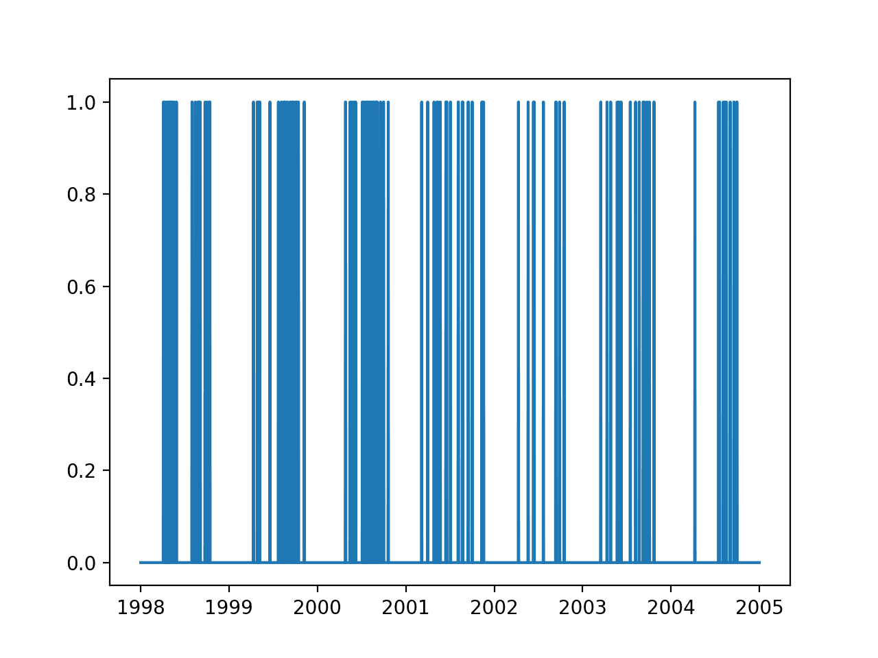
Line plot of output variable over 7 years

From briefly reviewing the observations, we can get some ideas of how we might prepare the data:

• Missing data requires handling.
• The simplest framing is to predict ozone day tomorrow based on observations today.
• Temperature is likely correlated with season or time of year and may be a useful predictor.
• Data variables may require scaling (normalization) and perhaps even standardization depending on the algorithm chosen.
• Predicting probabilities will provide more nuance than predicting class values.
• Perhaps we can use five years (about 72%) to train a model and test it on the remaining two years (about 28%)

We can perform some minimal data preparation.

The example below loads the dataset, replaces the missing observations with 0.0, frames the data as a supervised learning problem (predict ozone tomorrow based on observations today), and splits the data into train and test sets, based on a rough number of days in two years.

You could explore alternate approaches to replacing the missing values, such as imputing a mean value. Also, 2004 is a leap year, so the split of data into train and test sets is not a clean 5-2 year split, but is close enough for this tutorial.

Running the example saves the train and test sets to CSV files and summarizes the shape of the two datasets.

Naive Prediction Model

A naive model would predict the probability of an ozone day each day.

This is a naive approach because it does not use any information other than the base rate of the event. In the verification of meteorological forecasts, this is called the climatological forecast.

We can estimate the probability of an ozone day from the training dataset, as follows.

We can then predict the naive probability of an ozone day for each day on the test dataset.

Once we have a forecast, we can evaluate it.

A useful measure for evaluating probabilistic forecast is the Brier score. This score can be thought of as the mean squared error of the predicted probabilities (e.g. 5%) from the expected probabilities (0% or 1%). It is the average of the errors made across each day in the test dataset.

We are interested in minimizing the Brier score, smaller values are better, e.g. smaller error.

We can evaluate the Brier score for a forecast using the brier_score_loss() function from the scikit-learn library.

For a model to be skilful, it must have a score better than the score of the naive forecast.

We can make this obvious by calculating a Brier Skill Score (BSS) that normalizes the Brier Score (BS) based on the naive forecast.

We expect that the calculated BSS for the naive forecast would be 0.0. Going forward, we are interested in maximizing this score, e.g. larger BSS scores are better.

The complete example for the naive forecast is listed below.

Note: Your results may vary given the stochastic nature of the algorithm or evaluation procedure, or differences in numerical precision. Consider running the example a few times and compare the average outcome.

Running the example, we can see the naive probability of an ozone day even is about 7.2%.

Using the base rate as a forecast results in a Brier skill of 0.039 and the expected Brier Skill Score of 0.0 (ignore the sign).

We are now ready to explore some machine learning methods to see if we can add skill to this forecast.

Note that the original papers evaluated the skill of the approaches using precision and recall directly, a surprising approach for direct comparison between methods.

Perhaps an alternative measure you could explore is the area under ROC curve (ROC AUC). Plotting ROC curves for final models would allow the operator of the model to choose a threshold that provides the desired level of balance between the true positive (hit) and false positive (false alarm) rates.

Ensemble Tree Prediction Models

The original paper reports some success with bagged decision trees.

Though our choice of inductive learners are nonexhaustive, this paper has shown that inductive learning can be a method of choice for ozone level forecast, and ensemble-based probability trees provide better forecasts (higher recall and precision) than existing approaches.

— Forecasting Skewed Biased Stochastic Ozone Days: Analyses and Solutions, 2006.

This is not surprising for a few reasons:

• Bagged decision trees do not require any data scaling.
• Bagged decision trees automatically perform a type of feature section, ignoring irrelevant features.
• Bagged decision trees predict reasonably calibrated probabilities (e.g. unlike SVM).

This suggests a good place to start when testing machine learning algorithms on the problem.

We can get started quickly by spot-checking the performance of a sample of standard ensemble tree methods from the scikit-learn library with their default configurations and the number of trees set to 100.

Specifically, the methods:

• Bagged Decision Trees (BaggingClassifier)
• Extra Trees (ExtraTreesClassifier)
• Stochastic Gradient Boosting (GradientBoostingClassifier)
• Random Forest (RandomForestClassifier)

First, we must split the train and test datasets into input (X) and output (y) components so that we can fit sklearn models.

We also require the Brier Score for the naive forecast so that we can correctly calculate the Brier Skill Scores for the new models.

We can evaluate the skill of a single scikit-learn model generically.

Below defines the function named evaluate_once() that fits and evaluates a given defined and configured scikit-learn model and returns the Brier Skill Score (BSS).

Ensemble trees are a stochastic machine learning method.

This means that they will make different predictions when the same configuration of the same model is trained on the same data. To correct for this, we can evaluate a given model multiple times, such as 10 times, and calculate the average skill across each of these runs.

The function below will evaluate a given model 10 times, print the average BSS score, and return the population of scores for analysis.

We are now ready to evaluate a suite of ensemble decision tree algorithms.

The complete example is listed below.

Running the example summarizes the average BSS for each model averaged across 10 runs.

Note: Your results may vary given the stochastic nature of the algorithm or evaluation procedure, or differences in numerical precision. Consider running the example a few times and compare the average outcome.

From the mean BSS scores, it suggests that extra trees, stochastic gradient boosting, and random forest models are the most skillful.

A box and whisker plot of the scores for each model is plotted.

All of the models on all of their runs showed skill over the naive forecast (positive scores), which is very encouraging.

The distribution of the BSS scores for Extra Trees, Stochastic Gradient Boosting, and Random Forest all look encouraging.

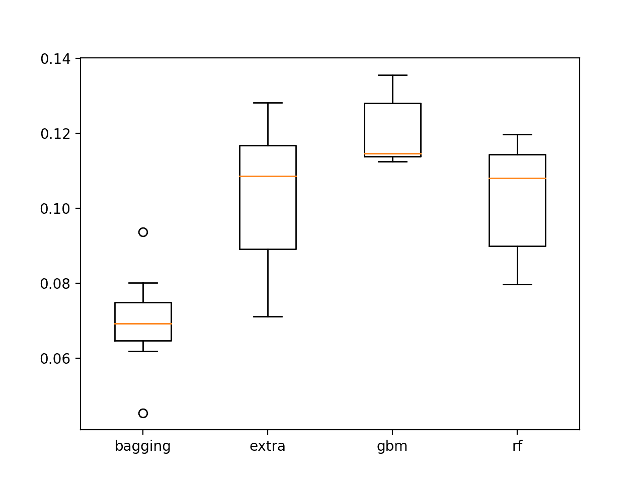
Box and whisker plot of ensemble decision tree BSS scores on the test set

Tune Gradient Boosting

Given that stochastic gradient boosting looks promising, it is worth exploring whether the performance of the model can be further lifted through some parameter tuning.

There are many parameters to tune with the model, but some good heuristics for tuning the model include:

• Decreasing the learning rate (learning_rate) while increasing the number of decision trees (n_estimators).
• Increasing the maximum depth of decision trees (max_depth) while also decreasing the number of samples that can be used to fit trees (samples).

Rather than grid searching values, we can spot check some arguments based on these principles. You can explore grid searching of these parameters yourself if you have the time and computational resources.

We will compare four configurations of the GBM model:

• baseline: as tested in the previous section (learning_rate=0.1, n_estimators=100, subsample=1.0, max_depth=3)
• lr, with lower learning rate and more trees (learning_rate=0.01, n_estimators=500, subsample=1.0, max_depth=3)
• depth, with increased maximum tree depth and smaller sampling of the dataset (learning_rate=0.1, n_estimators=100, subsample=0.7, max_depth=)
• all, with all of the modifications.

The complete example is listed below.

Running the example prints the BSS for each model averaged across 10 runs for each configuration.

Note: Your results may vary given the stochastic nature of the algorithm or evaluation procedure, or differences in numerical precision. Consider running the example a few times and compare the average outcome.

The results suggest that the change to the learning rate and number of trees alone introduced some lift over the default configuration.

The results also show that the ‘all’ configuration that included each change resulted in the best mean BSS.

Box and whisker plots of the BSS scores from each configuration are created. We can see that the configuration that included all the changes was dramatically better than the baseline model and the other configuration combinations.

Perhaps even further gains are possible with fine tuned arguments to the model.

Box and whisker plot of tuned GBM models showing BSS scores on the test set

It would be interesting to get a hold of the parametric model described in the paper and the data required to use it in order to compare its skill to the skill of this final model.

Extensions

This section lists some ideas for extending the tutorial that you may wish to explore.

• Explore a framing of the model that uses observations from multiple prior days.
• Explore model evaluations that use ROC curve plots and ROC AUC measures.
• Grid search the gradient boosting model arguments and perhaps explore other implementations such as XGBoost.

If you explore any of these extensions, I’d love to know.

Further Reading

This section provides more resources on the topic if you are looking to go deeper.

• Ozone Level Detection Data Set, UCI Machine Learning Repository.
• Forecasting Skewed Biased Stochastic Ozone Days: Analyses and Solutions, 2006.
• Forecasting skewed biased stochastic ozone days: analyses, solutions and beyond, 2008.
• CAWCR Verification Page
• Receiver operating characteristic on Wikipedia

Summary

In this tutorial, you discovered how to develop a probabilistic forecast model to predict air pollution in Houston, Texas.

Specifically, you learned:

• How to load and prepare the ozone day standard machine learning predictive modeling problem.
• How to develop a naive forecast model and evaluate the forecast using the Brier skill score.
• How to develop skilful models using ensembles of decision trees and further improve skill through hyperparameter tuning of a successful model.

Do you have any questions?
Ask your questions in the comments below and I will do my best to answer.

Develop Deep Learning models for Time Series Today!

Develop Your Own Forecasting models in Minutes

...with just a few lines of python code

Discover how in my new Ebook:
Deep Learning for Time Series Forecasting

It provides self-study tutorials on topics like:
CNNs, LSTMs, Multivariate Forecasting, Multi-Step Forecasting and much more...

Finally Bring Deep Learning to your Time Series Forecasting Projects

Skip the Academics. Just Results.

See What's Inside