Real-world time series forecasting is challenging for a whole host of reasons not limited to problem features such as having multiple input variables, the requirement to predict multiple time steps, and the need to perform the same type of prediction for multiple physical sites.
The EMC Data Science Global Hackathon dataset, or the ‘Air Quality Prediction‘ dataset for short, describes weather conditions at multiple sites and requires a prediction of air quality measurements over the subsequent three days.
An important first step when working with a new time series forecasting dataset is to develop a baseline in model performance by which the skill of all other more sophisticated strategies can be compared. Baseline forecasting strategies are simple and fast. They are referred to as ‘naive’ strategies because they assume very little or nothing about the specific forecasting problem.
In this tutorial, you will discover how to develop naive forecasting methods for the multistep multivariate air pollution time series forecasting problem.
After completing this tutorial, you will know:
How to develop a test harness for evaluating forecasting strategies for the air pollution dataset.
How to develop global naive forecast strategies that use data from the entire training dataset.
How to develop local naive forecast strategies that use data from the specific interval that is being forecasted.
Kick-start your project with my new book Deep Learning for Time Series Forecasting, including step-by-step tutorials and the Python source code files for all examples.
Let’s get started.
How to Develop Baseline Forecasts for Multi-Site Multivariate Air Pollution Time Series Forecasting Photo by DAVID HOLT, some rights reserved.
Tutorial Overview
This tutorial is divided into six parts; they are:
Problem Description
Naive Methods
Model Evaluation
Global Naive Methods
Chunk Naive Methods
Summary of Results
Problem Description
The Air Quality Prediction dataset describes weather conditions at multiple sites and requires a prediction of air quality measurements over the subsequent three days.
Specifically, weather observations such as temperature, pressure, wind speed, and wind direction are provided hourly for eight days for multiple sites. The objective is to predict air quality measurements for the next 3 days at multiple sites. The forecast lead times are not contiguous; instead, specific lead times must be forecast over the 72 hour forecast period. They are:
1
+1, +2, +3, +4, +5, +10, +17, +24, +48, +72
Further, the dataset is divided into disjoint but contiguous chunks of data, with eight days of data followed by three days that require a forecast.
Not all observations are available at all sites or chunks and not all output variables are available at all sites and chunks. There are large portions of missing data that must be addressed.
Submissions for the competition were evaluated against the true observations that were withheld from participants and scored using Mean Absolute Error (MAE). Submissions required the value of -1,000,000 to be specified in those cases where a forecast was not possible due to missing data. In fact, a template of where to insert missing values was provided and required to be adopted for all submissions (what a pain).
A winning entrant achieved a MAE of 0.21058 on the withheld test set (private leaderboard) using random forest on lagged observations. A writeup of this solution is available in the post:
In this tutorial, we will explore how to develop naive forecasts for the problem that can be used as a baseline to determine whether a model has skill on the problem or not.
Need help with Deep Learning for Time Series?
Take my free 7-day email crash course now (with sample code).
Click to sign-up and also get a free PDF Ebook version of the course.
Naive Forecast Methods
A baseline in forecast performance provides a point of comparison.
It is a point of reference for all other modeling techniques on your problem. If a model achieves performance at or below the baseline, the technique should be fixed or abandoned.
The technique used to generate a forecast to calculate the baseline performance must be easy to implement and naive of problem-specific details. The principle is that if a sophisticated forecast method cannot outperform a model that uses little or no problem-specific information, then it does not have skill.
There are problem-agnostic forecast methods that can and should be used first, followed by naive methods that use a modicum of problem-specific information.
Two examples of problem agnostic naive forecast methods that could be used include:
Persist the last observed value for each series.
Forecast the average of observed values for each series.
The data is divided into chunks, or intervals, of time. Each chunk of time has multiple variables at multiple sites to forecast. The persistence forecast method makes sense at this chunk-level of organization of the data.
Other persistence methods could be explored; for example:
Forecast observations from the previous day for the next three days for each series.
Forecast observations from the previous three days for the next three days for each series.
These are desirable baseline methods to explore, but the large amount of missing data and discontiguous structure of most of the data chunks make them challenging to implement without non-trivial data preparation.
Forecasting the average observations for each series can be elaborated further; for example:
Forecast the global (across-chunk) average value for each series.
Forecast the local (within-chunk) average value for each series.
A three-day forecast is required for each series with different start-times, e.g. times of day. As such, the forecast lead times for each chunk will fall on different hours of the day.
A further elaboration of forecasting the average value is to incorporate the hour of day that is being forecasted; for example:
Forecast the global (across-chunk) average value for the hour of day for each forecast lead time.
Forecast the local (within-chunk) average value for the hour of day for each forecast lead time.
Many variables are measured at multiple sites; as such, it may be possible to use information across series, such as in the calculation of averages or averages per hour of day for forecast lead times. These are interesting, but may exceed the mandate of naive.
This is a good starting point, although there may be further elaborations of the naive methods that you may want to consider and explore as an exercise. Remember, the goal is to use very little problem specific information in order to develop a forecast baseline.
In summary, we will investigate five different naive forecasting methods for this problem, the best of which will provide a lower-bound on performance by which other models can be compared. They are:
Global Average Value per Series
Global Average Value for Forecast Lead Time per Series
Local Persisted Value per Series
Local Average Value per Series
Local Average Value for Forecast Lead Time per Series
Model Evaluation
Before we can evaluate naive forecasting methods, we must develop a test harness.
This includes at least how the data will be prepared and how forecasts will be evaluated.
Load Dataset
The first step is to download the dataset and load it into memory.
The dataset can be downloaded for free from the Kaggle website. You may have to create an account and log in, in order to be able to download the dataset.
Download the entire dataset, e.g. “Download All” to your workstation and unzip the archive in your current working directory with the folder named ‘AirQualityPrediction‘.
Our focus will be the ‘TrainingData.csv‘ file that contains the training dataset, specifically data in chunks where each chunk is eight contiguous days of observations and target variables.
We can load the data file into memory using the Pandas read_csv() function and specify the header row on line 0.
Running the example prints the number of chunks in the dataset.
1
Total Chunks: 208
Data Preparation
Now that we know how to load the data and split it into chunks, we can separate into train and test datasets.
Each chunk covers an interval of eight days of hourly observations, although the number of actual observations within each chunk may vary widely.
We can split each chunk into the first five days of observations for training and the last three for test.
Each observation has a row called ‘position_within_chunk‘ that varies from 1 to 192 (8 days * 24 hours). We can therefore take all rows with a value in this column that is less than or equal to 120 (5 * 24) as training data and any values more than 120 as test data.
Further, any chunks that don’t have any observations in the train or test split can be dropped as not viable.
When working with the naive models, we are only interested in the target variables, and none of the input meteorological variables. Therefore, we can remove the input data and have the train and test data only comprised of the 39 target variables for each chunk, as well as the position within chunk and hour of observation.
The split_train_test() function below implements this behavior; given a dictionary of chunks, it will split each into a list of train and test chunk data.
We do not require the entire test dataset; instead, we only require the observations at specific lead times over the three day period, specifically the lead times:
1
+1, +2, +3, +4, +5, +10, +17, +24, +48, +72
Where, each lead time is relative to the end of the training period.
First, we can put these lead times into a function for easy reference:
1
2
3
# return a list of relative forecast lead times
def get_lead_times():
return[1,2,3,4,5,10,17,24,48,72]
Next, we can reduce the test dataset down to just the data at the preferred lead times.
We can do that by looking at the ‘position_within_chunk‘ column and using the lead time as an offset from the end of the training dataset, e.g. 120 + 1, 120 +2, etc.
If we find a matching row in the test set, it is saved, otherwise a row of NaN observations is generated.
The function to_forecasts() below implements this and returns a NumPy array with one row for each forecast lead time for each chunk.
1
2
3
4
5
6
7
8
9
10
11
12
13
14
15
16
17
18
19
20
21
22
23
24
25
# convert the rows in a test chunk to forecasts
def to_forecasts(test_chunks,row_in_chunk_ix=1):
# get lead times
lead_times=get_lead_times()
# first 5 days of hourly observations for train
cut_point=5*24
forecasts=list()
# enumerate each chunk
forrows intest_chunks:
chunk_id=rows[0,0]
# enumerate each lead time
fortau inlead_times:
# determine the row in chunk we want for the lead time
offset=cut_point+tau
# retrieve data for the lead time using row number in chunk
Running the example first comments that chunk 69 is removed from the dataset for having insufficient data.
We can then see that we have 42 columns in each of the train and test sets, one for the chunk id, position within chunk, hour of day, and the 39 training variables.
We can also see the dramatically smaller version of the test dataset with rows only at the forecast lead times.
The new train and test datasets are saved in the ‘naive_train.csv‘ and ‘naive_test.csv‘ files respectively.
1
2
3
>dropping chunk=69: train=(0, 95), test=(28, 95)
Train Rows: (23514, 42)
Test Rows: (2070, 42)
Forecast Evaluation
Once forecasts have been made, they need to be evaluated.
It is helpful to have a simpler format when evaluating forecasts. For example, we will use the three-dimensional structure of [chunks][variables][time], where variable is the target variable number from 0 to 38 and time is the lead time index from 0 to 9.
Models are expected to make predictions in this format.
We can also restructure the test dataset to have this dataset for comparison. The prepare_test_forecasts() function below implements this.
1
2
3
4
5
6
7
8
9
10
11
12
13
# convert the test dataset in chunks to [chunk][variable][time] format
def prepare_test_forecasts(test_chunks):
predictions=list()
# enumerate chunks to forecast
forrows intest_chunks:
# enumerate targets for chunk
chunk_predictions=list()
forjinrange(3,rows.shape[1]):
yhat=rows[:,j]
chunk_predictions.append(yhat)
chunk_predictions=array(chunk_predictions)
predictions.append(chunk_predictions)
returnarray(predictions)
We will evaluate a model using the mean absolute error, or MAE. This is the metric that was used in the competition and is a sensible choice given the non-Gaussian distribution of the target variables.
If a lead time contains no data in the test set (e.g. NaN), then no error will be calculated for that forecast. If the lead time does have data in the test set but no data in the forecast, then the full magnitude of the observation will be taken as error. Finally, if the test set has an observation and a forecast was made, then the absolute difference will be recorded as the error.
The calculate_error() function implements these rules and returns the error for a given forecast.
1
2
3
4
5
6
7
# calculate the error between an actual and predicted value
def calculate_error(actual,predicted):
# give the full actual value if predicted is nan
ifisnan(predicted):
returnabs(actual)
# calculate abs difference
returnabs(actual-predicted)
Errors are summed across all chunks and all lead times, then averaged.
The overall MAE will be calculated, but we will also calculate a MAE for each forecast lead time. This can help with model selection generally as some models may perform differently at different lead times.
The evaluate_forecasts() function below implements this, calculating the MAE and per-lead time MAE for the provided predictions and expected values in [chunk][variable][time] format.
1
2
3
4
5
6
7
8
9
10
11
12
13
14
15
16
17
18
19
20
21
22
23
24
25
26
27
28
# evaluate a forecast in the format [chunk][variable][time]
We are now ready to start exploring the performance of naive forecasting methods.
Global Naive Methods
In this section, we will explore naive forecast methods that use all data in the training dataset, not constrained to the chunk for which we are making a prediction.
We will look at two approaches:
Forecast Average Value per Series
Forecast Average Value for Hour-of-Day per Series
Forecast Average Value per Series
The first step is to implement a general function for making a forecast for each chunk.
The function takes the training dataset and the input columns (chunk id, position in chunk, and hour) for the test set and returns forecasts for all chunks with the expected 3D format of [chunk][variable][time].
The function enumerates the chunks in the forecast, then enumerates the 39 target columns, calling another new function named forecast_variable() in order to make a prediction for each lead time for a given target variable.
The complete function is listed below.
1
2
3
4
5
6
7
8
9
10
11
12
13
14
# forecast for each chunk, returns [chunk][variable][time]
We can now implement a version of the forecast_variable() that calculates the mean for a given series and forecasts that mean for each lead time.
First, we must collect all observations in the target column across all chunks, then calculate the average of the observations while also ignoring the NaN values. The nanmean() NumPy function will calculate the mean of an array and ignore NaN values.
The forecast_variable() function below implements this behavior.
Note: Your results may vary given the stochastic nature of the algorithm or evaluation procedure, or differences in numerical precision. Consider running the example a few times and compare the average outcome.
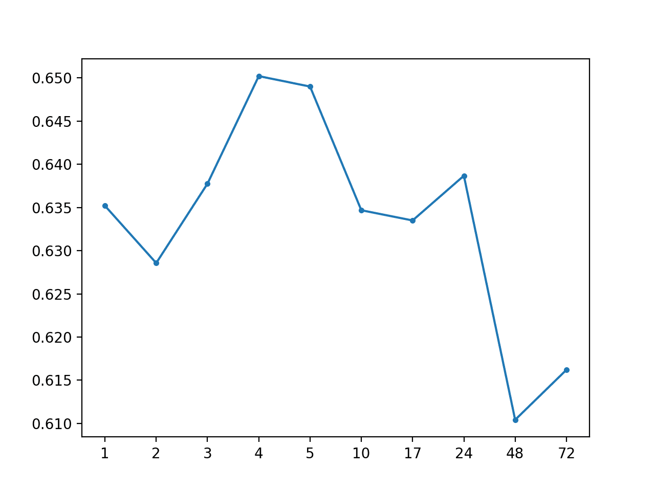
Running the example first prints the overall MAE of 0.634, followed by the MAE scores for each forecast lead time.
A line plot is created showing the MAE scores for each forecast lead time from +1 hour to +72 hours.
We cannot see any obvious relationship in forecast lead time to forecast error as we might expect with a more skillful model.
MAE by Forecast Lead Time With Global Mean
We can update the example to forecast the global median instead of the mean.
The median may make more sense to use as a central tendency than the mean for this data given the non-Gaussian like distribution the data seems to show.
NumPy provides the nanmedian() function that we can use in place of nanmean() in the forecast_variable() function.
The complete updated example is listed below.
1
2
3
4
5
6
7
8
9
10
11
12
13
14
15
16
17
18
19
20
21
22
23
24
25
26
27
28
29
30
31
32
33
34
35
36
37
38
39
40
41
42
43
44
45
46
47
48
49
50
51
52
53
54
55
56
57
58
59
60
61
62
63
64
65
66
67
68
69
70
71
72
73
74
75
76
77
78
79
80
81
82
83
84
85
86
87
88
89
90
91
92
93
94
95
96
97
98
99
100
101
102
103
104
105
106
107
108
109
110
111
112
113
114
115
116
117
118
119
120
121
122
123
124
125
126
127
128
# forecast global median
from numpy import loadtxt
from numpy import nan
from numpy import isnan
from numpy import count_nonzero
from numpy import unique
from numpy import array
from numpy import nanmedian
from matplotlib import pyplot
# split the dataset by 'chunkID', return a list of chunks
Note: Your results may vary given the stochastic nature of the algorithm or evaluation procedure, or differences in numerical precision. Consider running the example a few times and compare the average outcome.
Running the example shows a drop in MAE to about 0.59, suggesting that indeed using the median as the central tendency may be a better baseline strategy.
We can update the naive model for calculating a central tendency by series to only include rows that have the same hour of day as the forecast lead time.
For example, if the +1 lead time has the hour 6 (e.g. 0600 or 6AM), then we can find all other rows in the training dataset across all chunks for that hour and calculate the median value for a given target variable from those rows.
We record the hour of day on the test dataset and make it available to the model when making forecasts. One wrinkle is that in some cases the test dataset did not have a record for a given lead time and one had to be invented with NaN values, including a NaN value for the hour. In these cases, no forecast is required so we will skip them and forecast a NaN value.
The forecast_variable() function below implements this behavior, returning forecasts for each lead time for a given variable.
It is not very efficient, and it might be a lot more efficient to pre-calculate the median values for each hour for each variable first and then forecast using a lookup table. Efficiency is not a concern at this point as we are looking for a baseline of model performance.
summarize_error('Global Median by Hour',total_mae,times_mae)
Note: Your results may vary given the stochastic nature of the algorithm or evaluation procedure, or differences in numerical precision. Consider running the example a few times and compare the average outcome.
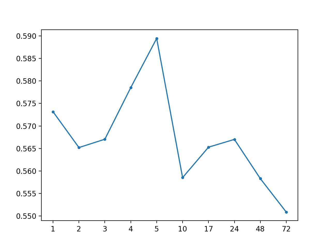
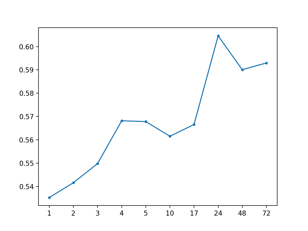
Running the example summarizes the performance of the model with a MAE of 0.567, which is an improvement over the global median for each series.
1
Global Median by Hour: [0.567 MAE] +1 0.573, +2 0.565, +3 0.567, +4 0.579, +5 0.589, +10 0.559, +17 0.565, +24 0.567, +48 0.558, +72 0.551
A line plot of the MAE by forecast lead time is also created showing that +72 had the lowest overall forecast error. This is interesting, and may suggest that hour-based information may be useful in more sophisticated models.
MAE by Forecast Lead Time With Global Median By Hour of Day
Chunk Naive Methods
It is possible that using information specific to the chunk may have more predictive power than using global information from the entire training dataset.
We can explore this with three local or chunk-specific naive forecasting methods; they are:
Forecast Last Observation per Series
Forecast Average Value per Series
Forecast Average Value for Hour-of-Day per Series
The last two of which are the chunk-specific version of the global strategies that were evaluated in the previous section.
Forecast Last Observation per Series
Forecasting the last non-NaN observation for a chunk is perhaps the simplest model, classically called the persistence model or the naive model.
The forecast_variable() function below implements this forecast strategy.
Running the example prints the overall MAE and the MAE per forecast lead time.
Note: Your results may vary given the stochastic nature of the algorithm or evaluation procedure, or differences in numerical precision. Consider running the example a few times and compare the average outcome.
We can see that the persistence forecast appears to out-perform all of the global strategies evaluated in the previous section.
This adds some support that the reasonable assumption that chunk-specific information is important in modeling this problem.
A line plot of MAE per forecast lead time is created.
Importantly, this plot shows the expected behavior of increasing error with the increase in forecast lead time. Namely, the further one predicts into the future, the more challenging it is, and in turn, the more error one would be expected to make.
MAE by Forecast Lead Time via Persistence
Forecast Average Value per Series
Instead of persisting the last observation for the series, we can persist the average value for the series using only the data in the chunk.
Specifically, we can calculate the median of the series, which as we found in the previous section seems to lead to better performance.
The forecast_variable() implements this local strategy.
Note: Your results may vary given the stochastic nature of the algorithm or evaluation procedure, or differences in numerical precision. Consider running the example a few times and compare the average outcome.
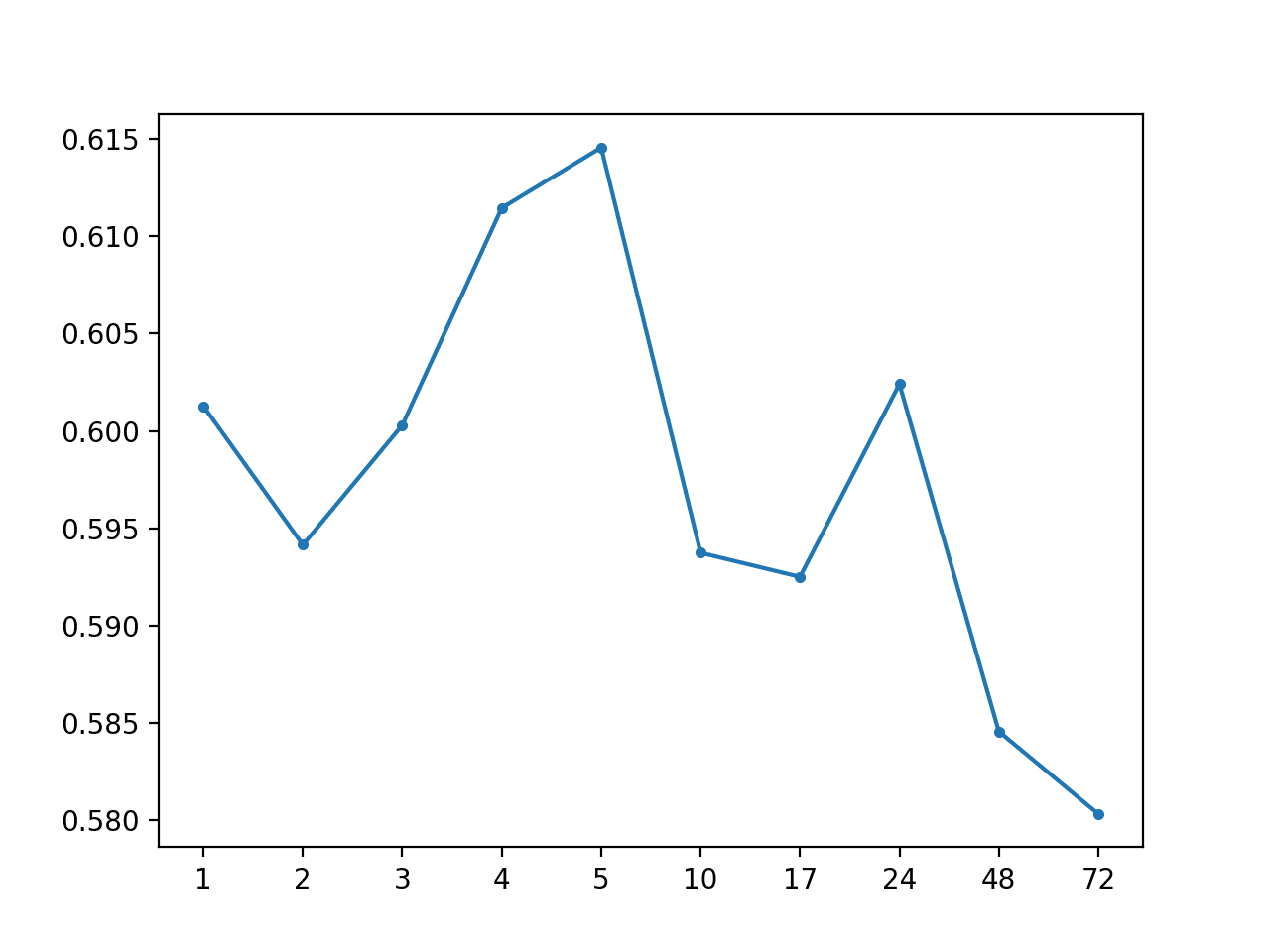
Running the example summarizes the performance of this naive strategy, showing a MAE of about 0.568, which is worse than the above persistence strategy.
A line plot of MAE per forecast lead time is also created showing the familiar increasing curve of error per lead time.
MAE by Forecast Lead Time via Local Median
Forecast Average Value for Hour-of-Day per Series
Finally, we can dial in the persistence strategy by using the average value per series for the specific hour of day at each forecast lead time.
This approach was found to be effective at the global strategy. It may be effective using only the data from the chunk, although at the risk of using a much smaller data sample.
The forecast_variable() function below implements this strategy, first finding all rows with the hour of the forecast lead time, then calculating the median of those rows for the given target variable.
summarize_error('Local Median by Hour',total_mae,times_mae)
Note: Your results may vary given the stochastic nature of the algorithm or evaluation procedure, or differences in numerical precision. Consider running the example a few times and compare the average outcome.
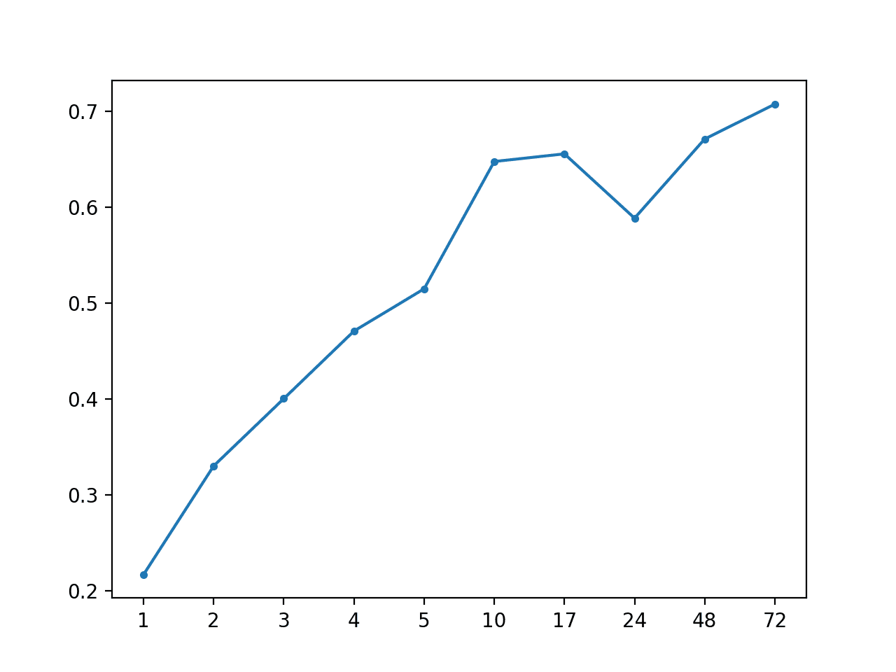
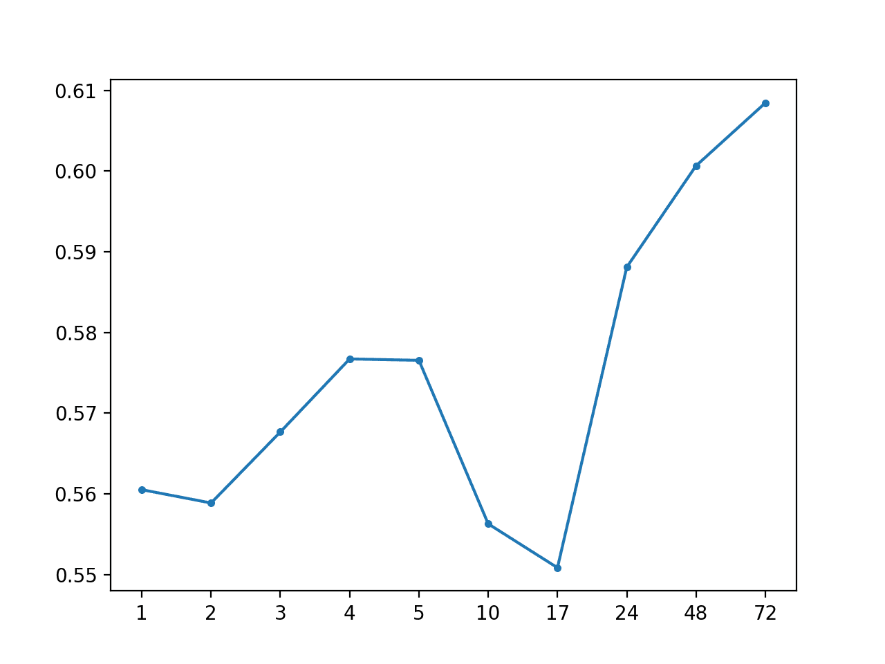
Running the example prints the overall MAE of about 0.574, which is worse than the global variation of the same strategy.
As suspected, this is likely due to the small sample size, that is at most five rows of training data contributing to each forecast.
1
Local Median by Hour: [0.574 MAE] +1 0.561, +2 0.559, +3 0.568, +4 0.577, +5 0.577, +10 0.556, +17 0.551, +24 0.588, +48 0.601, +72 0.608
A line plot of MAE per forecast lead time is also created showing the familiar increasing curve of error per lead time.
MAE by Forecast Lead Time via Local Median By Hour of Day
Summary of Results
We can summarize the performance of all of the naive forecast methods reviewed in this tutorial.
The example below lists each method using a shorthand of ‘g‘ and ‘l‘ for global and local and ‘h‘ for the hour-of-day variations. The example creates a bar chart so that we can compare the naive strategies based on their relative performance.
1
2
3
4
5
6
7
8
9
10
11
12
13
14
15
# summary of results
from matplotlib import pyplot
# results
results={
'g-mean':0.634,
'g-med':0.598,
'g-med-h':0.567,
'l-per':0.520,
'l-med':0.568,
'l-med-h':0.574}
# plot
pyplot.bar(results.keys(),results.values())
locs,labels=pyplot.xticks()
pyplot.setp(labels,rotation=30)
pyplot.show()
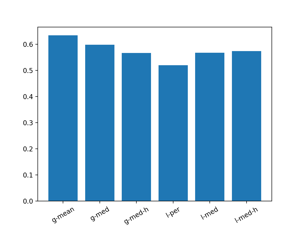
Running the example creates a bar chart comparing the MAE for each of the six strategies.
We can see that the persistence strategy was better than all of the other methods and that the second best strategy was the global median for each series that used the hour of day.
Models evaluated on this train/test separation of the dataset must achieve an overall MAE lower than 0.520 in order to be considered skillful.
Bar Chart with Summary of Naive Forecast Methods
Extensions
This section lists some ideas for extending the tutorial that you may wish to explore.
Cross-Site Naive Forecast. Develop a naive forecast strategy that uses information about each variable across sites, e.g. different target variables for the same variable at different sites.
Hybrid Approach. Develop a hybrid forecast strategy that combines elements of two or more of the naive forecast strategies at different lead times described in this tutorial.
Ensemble of Naive Methods. Develop an ensemble forecast strategy that creates a linear combination of two or more forecast strategies described in this tutorial.
If you explore any of these extensions, I’d love to know.
Further Reading
This section provides more resources on the topic if you are looking to go deeper.
In this tutorial, you discovered how to develop naive forecasting methods for the multistep multivariate air pollution time series forecasting problem.
Specifically, you learned:
How to develop a test harness for evaluating forecasting strategies for the air pollution dataset.
How to develop global naive forecast strategies that use data from the entire training dataset.
How to develop local naive forecast strategies that use data from the specific interval that is being forecasted.
Do you have any questions?
Ask your questions in the comments below and I will do my best to answer.
Develop Deep Learning models for Time Series Today!
Hi,
Thanks for a great tutorial. Just a small remark – to me, it would be much easier/quicker to understand steps if use pandas dataframes.
All the best!
A time to predict in the future relative to the current time.
It’s an abstraction, a symbolic time.
E.g. a lead time of +10 means predicting 10 time units into the future, regardless of what data we want to use to make the prediction or when we make the prediction.
A lead time of +25 hours means we are intersted in a model that can make a prediction one day or 24 hours out regardless of when we want to make a prediction.
Do you have any LSTM examples where you solve a multi-site multivariate multistep prediction problem? Or is it even a good idea to solve these types of problems using LSTMs?
I have a multivariate dataset from multiple sites. I currently make multistep predictions from 1 site using LSTMs, but I would like to incoorporate the data from all sites into a single model, so I can generalise my model to work at all sites.


Exactly how does this:
chunk_ids = unique(values[:, 1])
develop a list of unique identifiers?
When I see ‘unique’ I think set(). I am not following the above line of code.
Yes, a set, in this case a list of unique values in column 1.
Hi,
Thanks for a great tutorial. Just a small remark – to me, it would be much easier/quicker to understand steps if use pandas dataframes.
All the best!
Thanks.
what’s lead time?
A time to predict in the future relative to the current time.
It’s an abstraction, a symbolic time.
E.g. a lead time of +10 means predicting 10 time units into the future, regardless of what data we want to use to make the prediction or when we make the prediction.
A lead time of +25 hours means we are intersted in a model that can make a prediction one day or 24 hours out regardless of when we want to make a prediction.
Hi Jason,
I don’t understand why the lead time must be ‘+1, +2, +3, +4, +5, +10, +17, +24, +48, +72’ ?
Thank you.
They are a positive time relative to the current time.
You could choose other times, in this problem these lead times were chosen.
Does that help?
It helps. Thanks!
Hi Jason,
Thank you for your great posts.
Do you have any LSTM examples where you solve a multi-site multivariate multistep prediction problem? Or is it even a good idea to solve these types of problems using LSTMs?
I have a multivariate dataset from multiple sites. I currently make multistep predictions from 1 site using LSTMs, but I would like to incoorporate the data from all sites into a single model, so I can generalise my model to work at all sites.
I don’t know where to start.
Thanks
I have some advice on the topic here:
https://machinelearningmastery.com/faq/single-faq/how-to-develop-forecast-models-for-multiple-sites