How to Model Residual Errors to Correct Time Series Forecasts with Python

By Jason Brownlee on January 11, 2017 in Time Series

Last Updated on April 24, 2020

The residual errors from forecasts on a time series provide another source of information that we can model.

Residual errors themselves form a time series that can have temporal structure. A simple autoregression model of this structure can be used to predict the forecast error, which in turn can be used to correct forecasts. This type of model is called a moving average model, the same name but very different from moving average smoothing.

In this tutorial, you will discover how to model a residual error time series and use it to correct predictions with Python.

After completing this tutorial, you will know:

About how to model residual error time series using an autoregressive model.
How to develop and evaluate a model of residual error time series.
How to use a model of residual error to correct predictions and improve forecast skill.

Kick-start your project with my new book Time Series Forecasting With Python, including step-by-step tutorials and the Python source code files for all examples.

Let’s get started.

Updated Jan/2017: Improved some of the code examples to be more complete.
Updated Apr/2019: Updated the link to dataset.
Updated Aug/2019: Updated data loading to use new API.
Updated Apr/2020: Changed AR to AutoReg due to API change.

Model of Residual Errors

The difference between what was expected and what was predicted is called the residual error.

It is calculated as:

residual error = expected - predicted

1	residual error = expected - predicted

Just like the input observations themselves, the residual errors from a time series can have temporal structure like trends, bias, and seasonality.

Any temporal structure in the time series of residual forecast errors is useful as a diagnostic as it suggests information that could be incorporated into the predictive model. An ideal model would leave no structure in the residual error, just random fluctuations that cannot be modeled.

Structure in the residual error can also be modeled directly. There may be complex signals in the residual error that are difficult to directly incorporate into the model. Instead, you can create a model of the residual error time series and predict the expected error for your model.

The predicted error can then be subtracted from the model prediction and in turn provide an additional lift in performance.

A simple and effective model of residual error is an autoregression. This is where some number of lagged error values are used to predict the error at the next time step. These lag errors are combined in a linear regression model, much like an autoregression model of the direct time series observations.

An autoregression of the residual error time series is called a Moving Average (MA) model. This is confusing because it has nothing to do with the moving average smoothing process. Think of it as the sibling to the autoregressive (AR) process, except on lagged residual error rather than lagged raw observations.

In this tutorial, we will develop an autoregression model of the residual error time series.

Before we dive in, let’s look at a univariate dataset for which we will develop a model.

Stop learning Time Series Forecasting the slow way!

Take my free 7-day email course and discover how to get started (with sample code).

Click to sign-up and also get a free PDF Ebook version of the course.

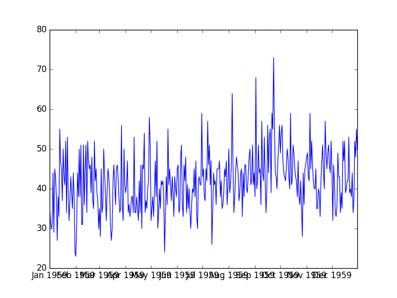
Daily Female Births Dataset

This dataset describes the number of daily female births in California in 1959.

The units are a count and there are 365 observations. The source of the dataset is credited to Newton (1988).

Download the dataset.

Download the dataset and place it in your current working directory with the filename “daily-total-female-births.csv“.

Below is an example of loading the Daily Female Births dataset from CSV.

from pandas import read_csv
from matplotlib import pyplot
series = read_csv('daily-total-female-births.csv', header=0, index_col=0)
print(series.head())
series.plot()
pyplot.show()

from pandas import read_csv

from matplotlib import pyplot

series = read_csv('daily-total-female-births.csv', header=0, index_col=0)

print(series.head())

series.plot()

pyplot.show()

Running the example prints the first 5 rows of the loaded file.

Date
1959-01-01 35
1959-01-02 32
1959-01-03 30
1959-01-04 31
1959-01-05 44
Name: Births, dtype: int64

Date

1959-01-01 35

1959-01-02 32

1959-01-03 30

1959-01-04 31

1959-01-05 44

Name: Births, dtype: int64

The dataset is also shown in a line plot of observations over time.

Daily Total Female Births Plot

We can see that there is no obvious trend or seasonality. The dataset looks stationary, which is an expectation of using an autoregression model.

Persistence Forecast Model

The simplest forecast that we can make is to forecast that what happened in the previous time step will be the same as what will happen in the next time step.

This is called the “naive forecast” or the persistence forecast model. This model will provide the predictions from which we can calculate the residual error time series. Alternately, we could develop an autoregression model of the time series and use that as our model. We will not develop an autoregression model in this case for brevity and to focus on the model of residual error.

We can implement the persistence model in Python.

After the dataset is loaded, it is phrased as a supervised learning problem. A lagged version of the dataset is created where the prior time step (t-1) is used as the input variable and the next time step (t+1) is taken as the output variable.

# create lagged dataset
values = DataFrame(series.values)
dataframe = concat([values.shift(1), values], axis=1)
dataframe.columns = ['t-1', 't+1']

# create lagged dataset

values = DataFrame(series.values)

dataframe = concat([values.shift(1), values], axis=1)

dataframe.columns = ['t-1', 't+1']

Next, the dataset is split into training and test sets. A total of 66% of the data is kept for training and the remaining 34% is held for the test set. No training is required for the persistence model; this is just a standard test harness approach.

Once split, the train and test sets are separated into their input and output components.

# split into train and test sets
X = dataframe.values
train_size = int(len(X) * 0.66)
train, test = X[1:train_size], X[train_size:]
train_X, train_y = train[:,0], train[:,1]
test_X, test_y = test[:,0], test[:,1]

# split into train and test sets

X = dataframe.values

train_size = int(len(X) * 0.66)

train, test = X[1:train_size], X[train_size:]

train_X, train_y = train[:,0], train[:,1]

test_X, test_y = test[:,0], test[:,1]

The persistence model is applied by predicting the output value (y) as a copy of the input value (x).

# persistence model
predictions = [x for x in test_X]

1 2	# persistence model predictions = [x for x in test_X]

The residual errors are then calculated as the difference between the expected outcome (test_y) and the prediction (predictions).

# calculate residuals
residuals = [test_y[i]-predictions[i] for i in range(len(predictions))]

1 2	# calculate residuals residuals = [test_y[i]-predictions[i] for i in range(len(predictions))]

The example puts this all together and gives us a set of residual forecast errors that we can explore this tutorial.

# calculate residual errors for a persistence forecast model
from pandas import read_csv
from pandas import DataFrame
from pandas import concat
from sklearn.metrics import mean_squared_error
from math import sqrt
# load data
series = read_csv('daily-total-female-births.csv', header=0, index_col=0, parse_dates=True, squeeze=True)
# create lagged dataset
values = DataFrame(series.values)
dataframe = concat([values.shift(1), values], axis=1)
dataframe.columns = ['t', 't+1']
# split into train and test sets
X = dataframe.values
train_size = int(len(X) * 0.66)
train, test = X[1:train_size], X[train_size:]
train_X, train_y = train[:,0], train[:,1]
test_X, test_y = test[:,0], test[:,1]
# persistence model
predictions = [x for x in test_X]
# skill of persistence model
rmse = sqrt(mean_squared_error(test_y, predictions))
print('Test RMSE: %.3f' % rmse)
# calculate residuals
residuals = [test_y[i]-predictions[i] for i in range(len(predictions))]
residuals = DataFrame(residuals)
print(residuals.head())

# calculate residual errors for a persistence forecast model

from pandas import read_csv

from pandas import DataFrame

from pandas import concat

from sklearn.metrics import mean_squared_error

from math import sqrt

# load data

series = read_csv('daily-total-female-births.csv', header=0, index_col=0, parse_dates=True, squeeze=True)

# create lagged dataset

values = DataFrame(series.values)

dataframe = concat([values.shift(1), values], axis=1)

dataframe.columns = ['t', 't+1']

# split into train and test sets

X = dataframe.values

train_size = int(len(X) * 0.66)

train, test = X[1:train_size], X[train_size:]

train_X, train_y = train[:,0], train[:,1]

test_X, test_y = test[:,0], test[:,1]

# persistence model

predictions = [x for x in test_X]

# skill of persistence model

rmse = sqrt(mean_squared_error(test_y, predictions))

print('Test RMSE: %.3f' % rmse)

# calculate residuals

residuals = [test_y[i]-predictions[i] for i in range(len(predictions))]

residuals = DataFrame(residuals)

print(residuals.head())

The example then prints the RMSE and the first 5 rows of the forecast residual errors.

Test RMSE: 9.151
      0
0   9.0
1 -10.0
2   3.0
3  -6.0
4  30.0

Test RMSE: 9.151

0 9.0

1 -10.0

2 3.0

3 -6.0

4 30.0

We now have a residual error time series that we can model.

Autoregression of Residual Error

We can model the residual error time series using an autoregression model.

This is a linear regression model that creates a weighted linear sum of lagged residual error terms. For example:

error(t+1) = b0 + b1*error(t-1) + b2*error(t-2) ...+ bn*error(t-n)

1	error(t+1) = b0 + b1error(t-1) + b2error(t-2) ...+ bn*error(t-n)

We can use the autoregression model (AR) provided by the statsmodels library.

Building on the persistence model in the previous section, we can first train the model on the residual errors calculated on the training dataset. This requires that we make persistence predictions for each observation in the training dataset, then create the AR model, as follows.

# autoregressive model of residual errors
from pandas import read_csv
from pandas import DataFrame
from pandas import concat
from statsmodels.tsa.ar_model import AutoReg
series = read_csv('daily-total-female-births.csv', header=0, index_col=0, parse_dates=True, squeeze=True)
# create lagged dataset
values = DataFrame(series.values)
dataframe = concat([values.shift(1), values], axis=1)
dataframe.columns = ['t', 't+1']
# split into train and test sets
X = dataframe.values
train_size = int(len(X) * 0.66)
train, test = X[1:train_size], X[train_size:]
train_X, train_y = train[:,0], train[:,1]
test_X, test_y = test[:,0], test[:,1]
# persistence model on training set
train_pred = [x for x in train_X]
# calculate residuals
train_resid = [train_y[i]-train_pred[i] for i in range(len(train_pred))]
# model the training set residuals
model = AutoReg(train_resid, lags=15)
model_fit = model.fit()
print('Coef=%s' % (model_fit.params))

# autoregressive model of residual errors

from pandas import read_csv

from pandas import DataFrame

from pandas import concat

from statsmodels.tsa.ar_model import AutoReg

series = read_csv('daily-total-female-births.csv', header=0, index_col=0, parse_dates=True, squeeze=True)

# create lagged dataset

values = DataFrame(series.values)

dataframe = concat([values.shift(1), values], axis=1)

dataframe.columns = ['t', 't+1']

# split into train and test sets

X = dataframe.values

train_size = int(len(X) * 0.66)

train, test = X[1:train_size], X[train_size:]

train_X, train_y = train[:,0], train[:,1]

test_X, test_y = test[:,0], test[:,1]

# persistence model on training set

train_pred = [x for x in train_X]

# calculate residuals

train_resid = [train_y[i]-train_pred[i] for i in range(len(train_pred))]

# model the training set residuals

model = AutoReg(train_resid, lags=15)

model_fit = model.fit()

print('Coef=%s' % (model_fit.params))

Running this piece prints the chosen lag of the 16 coefficients (intercept and one for each lag) of the trained linear regression model.

Coef=[ 0.10120699 -0.84940615 -0.77783609 -0.73345006 -0.68902061 -0.59270551
 -0.5376728  -0.42553356 -0.24861246 -0.19972102 -0.15954013 -0.11045476
 -0.14045572 -0.13299964 -0.12515801 -0.03615774]

Coef=[ 0.10120699 -0.84940615 -0.77783609 -0.73345006 -0.68902061 -0.59270551

-0.5376728 -0.42553356 -0.24861246 -0.19972102 -0.15954013 -0.11045476

-0.14045572 -0.13299964 -0.12515801 -0.03615774]

Next, we can step through the test dataset and for each time step we must:

Calculate the persistence prediction (t+1 = t-1).
Predict the residual error using the autoregression model.

The autoregression model requires the residual error of the 15 previous time steps. Therefore, we must keep these values handy.

As we step through the test dataset timestep by timestep making predictions and estimating error, we can then calculate the actual residual error and update the residual error time series lag values (history) so that we can calculate the error at the next time step.

This is a walk forward forecast, or a rolling forecast, model.

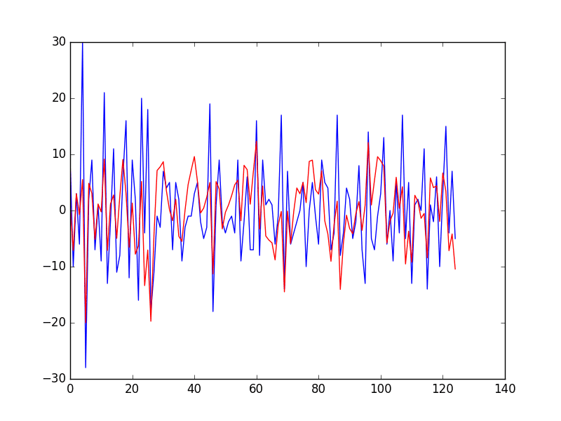
We end up with a time series of the residual forecast error from the train dataset and a predicted residual error on the test dataset.

We can plot these and get a quick idea of how skillful the model is at predicting residual error. The complete example is listed below.

# forecast residual forecast error
from pandas import read_csv
from pandas import DataFrame
from pandas import concat
from statsmodels.tsa.ar_model import AutoReg
from matplotlib import pyplot
series = read_csv('daily-total-female-births.csv', header=0, index_col=0, parse_dates=True, squeeze=True)
# create lagged dataset
values = DataFrame(series.values)
dataframe = concat([values.shift(1), values], axis=1)
dataframe.columns = ['t', 't+1']
# split into train and test sets
X = dataframe.values
train_size = int(len(X) * 0.66)
train, test = X[1:train_size], X[train_size:]
train_X, train_y = train[:,0], train[:,1]
test_X, test_y = test[:,0], test[:,1]
# persistence model on training set
train_pred = [x for x in train_X]
# calculate residuals
train_resid = [train_y[i]-train_pred[i] for i in range(len(train_pred))]
# model the training set residuals
window = 15
model = AutoReg(train_resid, lags=window)
model_fit = model.fit()
coef = model_fit.params
# walk forward over time steps in test
history = train_resid[len(train_resid)-window:]
history = [history[i] for i in range(len(history))]
predictions = list()
expected_error = list()
for t in range(len(test_y)):
	# persistence
	yhat = test_X[t]
	error = test_y[t] - yhat
	expected_error.append(error)
	# predict error
	length = len(history)
	lag = [history[i] for i in range(length-window,length)]
	pred_error = coef[0]
	for d in range(window):
		pred_error += coef[d+1] * lag[window-d-1]
	predictions.append(pred_error)
	history.append(error)
	print('predicted error=%f, expected error=%f' % (pred_error, error))
# plot predicted error
pyplot.plot(expected_error)
pyplot.plot(predictions, color='red')
pyplot.show()

# forecast residual forecast error

from pandas import read_csv

from pandas import DataFrame

from pandas import concat

from statsmodels.tsa.ar_model import AutoReg

from matplotlib import pyplot

series = read_csv('daily-total-female-births.csv', header=0, index_col=0, parse_dates=True, squeeze=True)

# create lagged dataset

values = DataFrame(series.values)

dataframe = concat([values.shift(1), values], axis=1)

dataframe.columns = ['t', 't+1']

# split into train and test sets

X = dataframe.values

train_size = int(len(X) * 0.66)

train, test = X[1:train_size], X[train_size:]

train_X, train_y = train[:,0], train[:,1]

test_X, test_y = test[:,0], test[:,1]

# persistence model on training set

train_pred = [x for x in train_X]

# calculate residuals

train_resid = [train_y[i]-train_pred[i] for i in range(len(train_pred))]

# model the training set residuals

window = 15

model = AutoReg(train_resid, lags=window)

model_fit = model.fit()

coef = model_fit.params

# walk forward over time steps in test

history = train_resid[len(train_resid)-window:]

history = [history[i] for i in range(len(history))]

predictions = list()

expected_error = list()

for t in range(len(test_y)):

# persistence

yhat = test_X[t]

error = test_y[t] - yhat

expected_error.append(error)

# predict error

length = len(history)

lag = [history[i] for i in range(length-window,length)]

pred_error = coef[0]

for d in range(window):

pred_error += coef[d+1] * lag[window-d-1]

predictions.append(pred_error)

history.append(error)

print('predicted error=%f, expected error=%f' % (pred_error, error))

# plot predicted error

pyplot.plot(expected_error)

pyplot.plot(predictions, color='red')

pyplot.show()

Running the example first prints the predicted and expected residual error for each time step in the test dataset.

...
predicted error=-1.951332, expected error=-10.000000
predicted error=6.675538, expected error=3.000000
predicted error=3.419129, expected error=15.000000
predicted error=-7.160046, expected error=-4.000000
predicted error=-4.179003, expected error=7.000000
predicted error=-10.425124, expected error=-5.000000

...

predicted error=-1.951332, expected error=-10.000000

predicted error=6.675538, expected error=3.000000

predicted error=3.419129, expected error=15.000000

predicted error=-7.160046, expected error=-4.000000

predicted error=-4.179003, expected error=7.000000

predicted error=-10.425124, expected error=-5.000000

Next, the actual residual error for the time series is plotted (blue) compared to the predicted residual error (red).

Prediction of Residual Error Time Series

Now that we know how to model residual error, next we will look at how we can go about correcting forecasts and improving model skill.

Correct Predictions with a Model of Residual Errors

A model of forecast residual error is interesting, but it can also be useful to make better predictions.

With a good estimate of forecast error at a time step, we can make better predictions.

For example, we can add the expected forecast error to a prediction to correct it and in turn improve the skill of the model.

improved forecast = forecast + estimated error

1	improved forecast = forecast + estimated error

Let’s make this concrete with an example.

Let’s say that the expected value for a time step is 10. The model predicts 8 and estimates the error to be 3. The improved forecast would be:

improved forecast = forecast + estimated error
improved forecast = 8 + 3
improved forecast = 11

improved forecast = forecast + estimated error

improved forecast = 8 + 3

improved forecast = 11

This takes the actual forecast error from 2 units to 1 unit.

We can update the example from the previous section to add the estimated forecast error to the persistence forecast as follows:

# correct the prediction
yhat = yhat + pred_error

1 2	# correct the prediction yhat = yhat + pred_error

The complete example is listed below.

# correct forecasts with a model of forecast residual errors
from pandas import read_csv
from pandas import DataFrame
from pandas import concat
from statsmodels.tsa.ar_model import AutoReg
from matplotlib import pyplot
from sklearn.metrics import mean_squared_error
from math import sqrt
# load data
series = read_csv('daily-total-female-births.csv', header=0, index_col=0, parse_dates=True, squeeze=True)
# create lagged dataset
values = DataFrame(series.values)
dataframe = concat([values.shift(1), values], axis=1)
dataframe.columns = ['t', 't+1']
# split into train and test sets
X = dataframe.values
train_size = int(len(X) * 0.66)
train, test = X[1:train_size], X[train_size:]
train_X, train_y = train[:,0], train[:,1]
test_X, test_y = test[:,0], test[:,1]
# persistence model on training set
train_pred = [x for x in train_X]
# calculate residuals
train_resid = [train_y[i]-train_pred[i] for i in range(len(train_pred))]
# model the training set residuals
window = 15
model = AutoReg(train_resid, lags=15)
model_fit = model.fit()
coef = model_fit.params
# walk forward over time steps in test
history = train_resid[len(train_resid)-window:]
history = [history[i] for i in range(len(history))]
predictions = list()
for t in range(len(test_y)):
	# persistence
	yhat = test_X[t]
	error = test_y[t] - yhat
	# predict error
	length = len(history)
	lag = [history[i] for i in range(length-window,length)]
	pred_error = coef[0]
	for d in range(window):
		pred_error += coef[d+1] * lag[window-d-1]
	# correct the prediction
	yhat = yhat + pred_error
	predictions.append(yhat)
	history.append(error)
	print('predicted=%f, expected=%f' % (yhat, test_y[t]))
# error
rmse = sqrt(mean_squared_error(test_y, predictions))
print('Test RMSE: %.3f' % rmse)
# plot predicted error
pyplot.plot(test_y)
pyplot.plot(predictions, color='red')
pyplot.show()

# correct forecasts with a model of forecast residual errors

from pandas import read_csv

from pandas import DataFrame

from pandas import concat

from statsmodels.tsa.ar_model import AutoReg

from matplotlib import pyplot

from sklearn.metrics import mean_squared_error

from math import sqrt

# load data

series = read_csv('daily-total-female-births.csv', header=0, index_col=0, parse_dates=True, squeeze=True)

# create lagged dataset

values = DataFrame(series.values)

dataframe = concat([values.shift(1), values], axis=1)

dataframe.columns = ['t', 't+1']

# split into train and test sets

X = dataframe.values

train_size = int(len(X) * 0.66)

train, test = X[1:train_size], X[train_size:]

train_X, train_y = train[:,0], train[:,1]

test_X, test_y = test[:,0], test[:,1]

# persistence model on training set

train_pred = [x for x in train_X]

# calculate residuals

train_resid = [train_y[i]-train_pred[i] for i in range(len(train_pred))]

# model the training set residuals

window = 15

model = AutoReg(train_resid, lags=15)

model_fit = model.fit()

coef = model_fit.params

# walk forward over time steps in test

history = train_resid[len(train_resid)-window:]

history = [history[i] for i in range(len(history))]

predictions = list()

for t in range(len(test_y)):

# persistence

yhat = test_X[t]

error = test_y[t] - yhat

# predict error

length = len(history)

lag = [history[i] for i in range(length-window,length)]

pred_error = coef[0]

for d in range(window):

pred_error += coef[d+1] * lag[window-d-1]

# correct the prediction

yhat = yhat + pred_error

predictions.append(yhat)

history.append(error)

print('predicted=%f, expected=%f' % (yhat, test_y[t]))

# error

rmse = sqrt(mean_squared_error(test_y, predictions))

print('Test RMSE: %.3f' % rmse)

# plot predicted error

pyplot.plot(test_y)

pyplot.plot(predictions, color='red')

pyplot.show()

Running the example prints the predictions and the expected outcome for each time step in the test dataset.

The RMSE of the corrected forecasts is calculated to be 7.499, which is much better than the score of 9.151 for the persistence model alone.

...
predicted=40.675538, expected=37.000000
predicted=40.419129, expected=52.000000
predicted=44.839954, expected=48.000000
predicted=43.820997, expected=55.000000
predicted=44.574876, expected=50.000000
Test RMSE: 7.499

...

predicted=40.675538, expected=37.000000

predicted=40.419129, expected=52.000000

predicted=44.839954, expected=48.000000

predicted=43.820997, expected=55.000000

predicted=44.574876, expected=50.000000

Test RMSE: 7.499

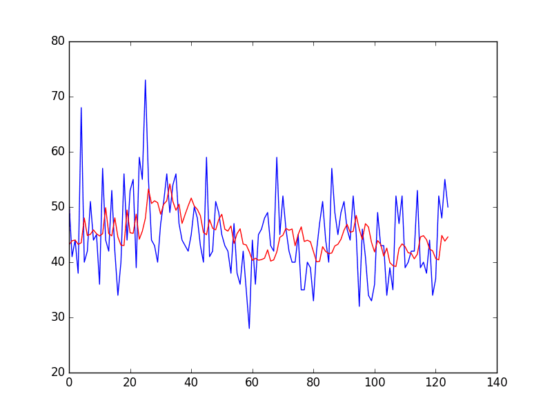
Finally, the expected values for the test dataset are plotted (blue) compared to the corrected forecast (red).

We can see that the persistence model has been aggressively corrected back to a time series that looks something like a moving average.

Corrected Persistence Forecast for Daily Female Births

Summary

In this tutorial, you discovered how to model residual error time series and use it to correct predictions with Python.

Specifically, you learned:

About the Moving Average (MA) approach to developing an autoregressive model to residual error.
How to develop and evaluate a model of residual error to predict forecast error.
How to use the predictions of forecast error to correct predictions and improve model skill.

Do you have any questions about Moving Average models, or about this tutorial?
Ask your questions in the comments below and I will do my best to answer.

61 Responses to How to Model Residual Errors to Correct Time Series Forecasts with Python

dj January 17, 2017 at 2:34 pm #

Is anyone else finding that these tutorials just don’t work?

Reply
- Jason Brownlee January 17, 2017 at 2:38 pm #
  
  Sorry to hear that, what problem are you getting exactly?
  
  Update: I updated the first two code examples to be more complete/easier to run directly.
  
  Reply
  - nanda December 19, 2019 at 6:35 pm #
    
    Hai jason, Is there any way to forecast auto correlated residual without having test data residuals
    
    Reply
    - Jason Brownlee December 20, 2019 at 6:41 am #
      
      Perhaps. You have complete freedom over how the problem is framed, e.g. the inputs and outputs.
      
      Be sure to choose inputs that you have available at prediction time.
      
      Reply
- lucy August 24, 2019 at 12:14 pm #
  
  hi,how to know lag numer?
  
  Reply
r4ever January 15, 2018 at 3:40 pm #

can I conclude above process as how arima(p,d,q) process works in background?

Reply
- Jason Brownlee January 16, 2018 at 7:30 am #
  
  Sorry, I don’t follow. Perhaps you can restate your question with more context?
  
  Reply
darkphoenix February 19, 2018 at 9:27 am #

i’m trying to model residual from arima using ann,it’s called hybrid arima. do you have any clue?

Reply
- Jason Brownlee February 19, 2018 at 10:39 am #
  
  What is the problem you are having exactly?
  
  Reply
  - Gurudev April 21, 2018 at 1:36 am #
    
    Sir Actually he is taking about Hybride ARIMA-ANN model G. Peter Zhang model in which residuals are modeled by ANN ..
    Problem is that how such small set of residuals are modeled by ANN…
    Thanks in advance
    
    Reply
Kue Bum Kim December 30, 2018 at 11:28 pm #

Thank you for the tutorial. Would you please explain this tutorial with matlab?

Reply
- Jason Brownlee December 31, 2018 at 6:10 am #
  
  Sorry, I don’t have matlab tutorials, it is a platform that is only used in school – not on business projects.
  
  Reply
Rima January 7, 2019 at 8:04 pm #

Hello Jason,
I used an SARIMAX model for my time series data and when calculating residual error for the test and train set, I observed a seasonality in the residual error. Do you think should I re-correct the SARIMAX model somehow or I can implement the above method you explained to the residual error?

Thank you Jason!
Have a good day.

PS: It will be useful to receive email from you whenever you reply to our messages.

Reply
- Jason Brownlee January 8, 2019 at 6:47 am #
  
  Yes, if there is a signal in the residual errors then the model should be updated to also cover that signal if possible.
  
  Reply
Fatima August 31, 2019 at 5:38 am #

Hello Jason,

“We can model the residual error time series using an autoregression model”

Would it be perhaps possible ( and more accurate) to model the residual error using a machine learning model?

Reply
- Jason Brownlee August 31, 2019 at 6:13 am #
  
  Why?
  
  Reply
  - Hiyam September 10, 2019 at 9:19 pm #
    
    Hello Jason, I wanted to ask the same question as Fatima.
    
    In my case, the dataset is actually multivariate, and I want to model the residual error on this multivariate dataset, and I assume the AR model won’t work in my case. Can I use the classical ML models for the same purpose ?
    
    Reply
    - Hiyam September 10, 2019 at 9:20 pm #
      
      Know that, I do have the lags included in my dataset
      
      Reply
    - Jason Brownlee September 11, 2019 at 5:34 am #
      
      Perhaps try a range of models including linear and machine learning and discover what works best for your specific dataset.
      
      Reply
Winnie September 12, 2019 at 1:28 am #

Hi Jason,
I do not quite understand how you got
‘next time step (t+1) is taken as the output variable’

It seems you used the values at time t as the values at time t+1.
Should it be ” values.shift(-1) ” ?

Thank you very much!

Reply
- Jason Brownlee September 12, 2019 at 5:20 am #
  
  Yes, I use t+1 for t. It was not a good choice of terminology.
  
  Reply
Row November 7, 2019 at 12:44 pm #

Hello Jason,
Thanks again for all your helpful tutorials!
I was reading about regression with ARMA errors on Rob Hyndman’s blog (https://robjhyndman.com/hyndsight/arimax/). Is it similar to what you have here except yours used a persistance model instead of ARMA / ARIMA?
Row

Reply
- Jason Brownlee November 7, 2019 at 2:06 pm #
  
  Yes, ARIMA is ARMA wit the added differencing step.
  
  Reply
Row November 7, 2019 at 2:47 pm #

Thank you, Jason.

Reply
- Jason Brownlee November 8, 2019 at 6:37 am #
  
  You’re welcome.
  
  Reply
Howbow December 4, 2019 at 10:36 pm #

Hi Jason,

thank you for posting this example.
In your example you are forecasting 1 step into the future, but what if you had to forecast lets say 10 steps ahead using this a persistence model combined with this error correction model?
Would you simply forecast the errors by changing the code to:

model_fit.forecast()[10] ?

In general, I think it would be useful if you would show an example of multiple steps ahead out of sample forecasts.

Cheers!

Reply
- Jason Brownlee December 5, 2019 at 6:41 am #
  
  Call model.forecsat(10)
  
  Reply
Shashank December 19, 2019 at 4:41 am #

history = train_resid[len(train_resid)-window:]
history = [history[i] for i in range(len(history))]

The first line outputs the same result as the second one. Could you explain why you have included them both? Thank you.

Reply
- Jason Brownlee December 19, 2019 at 6:34 am #
  
  Typo, I expect.
  
  Reply
  - Shashank December 19, 2019 at 9:08 am #
    
    Thanks for your reply. I made an ARIMA forecast for my dataset, for which I would like to forecast the errors too. Should I make a training set, fit the ARIMA model, forecast for the length of the test set and then get the errors from the test set? Or does it differ when using the ARIMA approach?
    
    Reply
    - Jason Brownlee December 19, 2019 at 12:48 pm #
      
      Yes, that sounds reasonable. Be sure to collect errors in the same way as obs, e.g. step-by-step or sequence by sequence.
      
      Reply
      - Shashank December 20, 2019 at 5:06 am #
        
        So I collected the errors step by step, and then checked for stationarity using the ADF and KPSS tests, which tell me that the errors are stationary. Then I fit an ARIMA(0, 0, 0) model on the errors after taking a look at the autocorrelation and partial autocorrelation plots. This model kind of averages out and is not very flexible, in the sense that it doesn’t capture spikes in the data, i.e., where the errors deviate a lot from the mean. Is there a way to fit a more flexible model or use a different one perhaps? Please let me know. Thanks!
      - Jason Brownlee December 20, 2019 at 6:53 am #
        
        Well done!
        
        Perhaps try a suite of models and model configurations and discover what works best for your dataset.
Adonis El Hajj March 18, 2020 at 5:53 pm #

Hi Jason,
is it possible to mix LSTM with a residual architecture?
thank you in advance.

Reply
- Jason Brownlee March 19, 2020 at 6:21 am #
  
  Yes, residual errors can be provided as input to the model.
  
  Reply
Saurabh April 7, 2020 at 8:50 am #

Hi Jason,

Thanks a lot for your work! Is it safe to assume that the process that you laid out in this blog is exactly what happens behind-the-scenes if I include an MA term in the ARIMA model?

Reply
- Jason Brownlee April 7, 2020 at 1:28 pm #
  
  Very close.
  
  Reply
Danilel May 1, 2020 at 3:13 am #

Hi Jason,

Contrasting the described 2-step approach of separately estimating models (first for response then for residuals) and subsequently combining them in the forecast step with estimation in the likes of GLMM or Transfer Functions Models where we (can) impose some correlation structure on the errors directly: are there any pitfalls if the practical objective is only a “good” forecast as measured here by RMSE (instead of say hypothesis testing on parameters)?

Thanks for your great work, I really appreciate it.

Reply
- Jason Brownlee May 1, 2020 at 6:45 am #
  
  Sorry, not sure I follow your question. Perhaps you can restate it?
  
  Reply
  - Danilel May 1, 2020 at 7:20 pm #
    
    In the article you say:
    “Structure in the residual error can also be modeled directly. There may be complex signals in the residual error that are difficult to directly incorporate into the model. Instead, you can create a model of the residual error time series and predict the expected error for your model.”
    
    Now the question is: in which cases is direct modelling of error structure preferred over the proposed 2-step method?
    
    I guess standard errors of parameters are affected, but is there any practical difference regarding forecast performance alone?
    
    Thanks
    
    Reply
    - Jason Brownlee May 2, 2020 at 5:42 am #
      
      No, use results/data to guide model selection.
      
      Perhaps try both approaches and use the model that has better skill/less error.
      
      Reply
TalaOwis May 9, 2020 at 2:04 am #

I was wondering if ARMARESULT.resid gives the actual residuals .I want to use those residuals in a different model .but the size of the array it return is 55 and the dataset I am fitting is 57 .

Reply
- Jason Brownlee May 9, 2020 at 6:19 am #
  
  Perhaps the model had a difference of 2 to account for the number of residuals?
  
  Reply
TalaOwis May 9, 2020 at 7:49 am #

you mean the q value is 2 ?

Reply
- TalaOwis May 9, 2020 at 7:59 am #
  
  If q is the reason why I am getting those results ,how would I align the residuals along with the time series data to feed them into another model like LSTM?
  If you can answer me and give me an example or any referrence I will be grateful .
  
  Reply
  - Jason Brownlee May 9, 2020 at 1:48 pm #
    
    I don’t have an example, you will have to experiment.
    
    Reply
- Jason Brownlee May 9, 2020 at 1:48 pm #
  
  Yes.
  
  Reply
Parth May 28, 2020 at 11:21 pm #

Good post. Have a question on 1 point.
Initially blog mentions this point

“There may be complex signals in the residual error that are difficult to directly incorporate into the model. ”

Regarding this, question is, can you share some ideas or techniques through which we can detect such structure in residual series. This will help to determine, if we need to do residual modelling or not, in first place.

Reply
- Jason Brownlee May 29, 2020 at 6:32 am #
  
  Sometimes, simply fitting a model on the residuals can lift performance.
  
  Reply
Vignesh Aravind June 28, 2020 at 8:48 am #

Hi Jason.. on the explanation about White noise… You mentioned that the only error after we extracted the signal from any time series should be White Noise. But that is the ideal model which we try to achieve…But there is always some Residual errors which we calculate from the Error measures like RSME… So basically any model would have both Residual errors which are reducible and White noise that are irreducible?
As George Box said “All models are wrong but some are useful”.

Reply
- Jason Brownlee June 29, 2020 at 6:24 am #
  
  Ideally we would get to the point where the residual error is comprise of white noise only.
  
  This is an ideal, not possible or very hard to achieve in practice.
  
  Reply
Pierre December 21, 2020 at 10:12 pm #

Hi Jason, thank you for your great explanation ! Some questions i got:

– Are these kind of methods working better for ‘dynamic environment’ (ie when possible cause of observed time serie change can change (new causes, …)) ? I mean if the environment is ‘stable’, should we not expect some white noise in the model ?

– Does this make sense to apply this method many times ? I mean checking to forecast the error of ‘second degree’ : ie error after adding the error forecast, and so on… I guess yes in theory if the second error is still not white noise, but does this really happen in practice ?

Reply
- Jason Brownlee December 22, 2020 at 6:45 am #
  
  It really depends on the specific of the dataset.
  
  Perhaps. Some experiemtantion may be required.
  
  Reply
  - Archana January 4, 2021 at 10:29 pm #
    
    Hi Jason,
    I am getting negative values for my sales prediction,can you plz suggest something to fix that especially in terms of tuning the hyperparameters.Just FYI, I am using azure automl to generate the model.
    
    Reply
    - Jason Brownlee January 5, 2021 at 6:22 am #
      
      Perhaps try an alternate model?
      Perhaps try an alternate configuration of your model?
      Perhaps try data preparation prior to modeling?
      Perhaps try post-processing of the predictions?
      
      Reply
XeXeeD February 17, 2021 at 6:47 pm #

Can you please add an option to sort the comments based on date pls. It really saves time.

Reply
- Jason Brownlee February 18, 2021 at 5:13 am #
  
  Comment threads are listed in date-time order ascending (oldest to newest).
  
  Reply
HooHuuKaa February 22, 2021 at 3:35 am #

I think this method doesn’t work. Main reason being using the expected error(ground truth) in the “history” list to predict the same thing. Multiplying the AutoReg coefs with pred_error, which remains prediction error only in the first loop. From next loop on-wards you’re using cheating.

Reply
- Ravi November 22, 2021 at 3:33 am #
  
  yes That’s true. after reading the comments I got to know that we can add prediction errors into history by actually predicting from AR model which trained on residual errors.
  
  Reply
shubham Gadhari November 24, 2021 at 7:31 pm #

Is this how we get residual terms in arima equation . Suppose ARIMA(2,0,4) model we can get the coefficients but model_fit.summary() I have the coefficient of 4 q terms but how are e(t-1) ,e(t-2) ,e(t-3) and e(t-4) is calculated . Will be very grateful if you can give relevant link

Reply
- Adrian Tam November 25, 2021 at 3:58 am #
  
  Error/residual terms are assumed to be random but following normal distribution. If you know the true value of x(t-1), x(t-2), etc. and compare too the prediction, then the difference is the error term. Otherwise, the error terms are unknown.
  
  Reply

Navigation

How to Model Residual Errors to Correct Time Series Forecasts with Python

Model of Residual Errors

Stop learning Time Series Forecasting the slow way!

Daily Female Births Dataset

Persistence Forecast Model

Autoregression of Residual Error

Correct Predictions with a Model of Residual Errors

Summary

Want to Develop Time Series Forecasts with Python?

Develop Your Own Forecasts in Minutes

Finally Bring Time Series Forecasting to
Your Own Projects

More On This Topic

61 Responses to How to Model Residual Errors to Correct Time Series Forecasts with Python

Leave a Reply Click here to cancel reply.

Navigation

Model of Residual Errors

Stop learning Time Series Forecasting the slow way!

Daily Female Births Dataset

Persistence Forecast Model

Autoregression of Residual Error

Correct Predictions with a Model of Residual Errors

Summary

Want to Develop Time Series Forecasts with Python?

Develop Your Own Forecasts in Minutes

Finally Bring Time Series Forecasting to Your Own Projects

More On This Topic

61 Responses to How to Model Residual Errors to Correct Time Series Forecasts with Python

Leave a Reply Click here to cancel reply.

Finally Bring Time Series Forecasting to
Your Own Projects