Making out-of-sample forecasts can be confusing when getting started with time series data.
The statsmodels Python API provides functions for performing one-step and multi-step out-of-sample forecasts.
In this tutorial, you will clear up any confusion you have about making out-of-sample forecasts with time series data in Python.
After completing this tutorial, you will know:
How to make a one-step out-of-sample forecast.
How to make a multi-step out-of-sample forecast.
The difference between the forecast() and predict() functions.
Kick-start your project with my new book Time Series Forecasting With Python, including step-by-step tutorials and the Python source code files for all examples.
Let’s get started.
Updated Apr/2019: Updated the link to dataset.
Updated Aug/2019: Updated data loading to use new API.
Updated Oct/2020: Updated file loading for changes to the API.
Updated Dec/2020: Updated ARIMA API to the latest version of statsmodels.
Updated Dec/2020: Fixed out of sample examples due to API changes.
How to Make Out-of-Sample Forecasts with ARIMA in Python Photo by dziambel, some rights reserved.
Tutorial Overview
This tutorial is broken down into the following 5 steps:
Dataset Description
Split Dataset
Develop Model
One-Step Out-of-Sample Forecast
Multi-Step Out-of-Sample Forecast
Stop learning Time Series Forecasting the slow way!
Take my free 7-day email course and discover how to get started (with sample code).
Click to sign-up and also get a free PDF Ebook version of the course.
1. Minimum Daily Temperatures Dataset
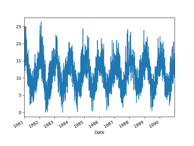
This dataset describes the minimum daily temperatures over 10 years (1981-1990) in the city of Melbourne, Australia.
The units are in degrees Celsius and there are 3,650 observations. The source of the data is credited as the Australian Bureau of Meteorology.
Running the example prints the first 20 rows of the loaded dataset.
1
2
3
4
5
6
7
8
9
10
11
12
13
14
15
16
17
18
19
20
21
Date
1981-01-01 20.7
1981-01-02 17.9
1981-01-03 18.8
1981-01-04 14.6
1981-01-05 15.8
1981-01-06 15.8
1981-01-07 15.8
1981-01-08 17.4
1981-01-09 21.8
1981-01-10 20.0
1981-01-11 16.2
1981-01-12 13.3
1981-01-13 16.7
1981-01-14 21.5
1981-01-15 25.0
1981-01-16 20.7
1981-01-17 20.6
1981-01-18 24.8
1981-01-19 17.7
1981-01-20 15.5
A line plot of the time series is also created.
Minimum Daily Temperatures Dataset Line Plot
2. Split Dataset
We can split the dataset into two parts.
The first part is the training dataset that we will use to prepare an ARIMA model. The second part is the test dataset that we will pretend is not available. It is these time steps that we will treat as out of sample.
The dataset contains data from January 1st 1981 to December 31st 1990.
We will hold back the last 7 days of the dataset from December 1990 as the test dataset and treat those time steps as out of sample.
Specifically 1990-12-25 to 1990-12-31:
1
2
3
4
5
6
7
1990-12-25,12.9
1990-12-26,14.6
1990-12-27,14.0
1990-12-28,13.6
1990-12-29,13.5
1990-12-30,15.7
1990-12-31,13.0
The code below will load the dataset, split it into the training and validation datasets, and save them to files dataset.csv and validation.csv respectively.
Run the example and you should now have two files to work with.
The last observation in the dataset.csv is Christmas Eve 1990:
1
1990-12-24,10.0
That means Christmas Day 1990 and onwards are out-of-sample time steps for a model trained on dataset.csv.
3. Develop Model
In this section, we are going to make the data stationary and develop a simple ARIMA model.
The data has a strong seasonal component. We can neutralize this and make the data stationary by taking the seasonal difference. That is, we can take the observation for a day and subtract the observation from the same day one year ago.
This will result in a stationary dataset from which we can fit a model.
1
2
3
4
5
6
7
# create a differenced series
def difference(dataset,interval=1):
diff=list()
foriinrange(interval,len(dataset)):
value=dataset[i]-dataset[i-interval]
diff.append(value)
returnnumpy.array(diff)
We can invert this operation by adding the value of the observation one year ago. We will need to do this to any forecasts made by a model trained on the seasonally adjusted data.
1
2
3
# invert differenced value
def inverse_difference(history,yhat,interval=1):
returnyhat+history[-interval]
We can fit an ARIMA model.
Fitting a strong ARIMA model to the data is not the focus of this post, so rather than going through the analysis of the problem or grid searching parameters, I will choose a simple ARIMA(7,0,7) configuration.
We can put all of this together as follows:
1
2
3
4
5
6
7
8
9
10
11
12
13
14
15
16
17
18
19
20
21
22
23
from pandas import read_csv
from statsmodels.tsa.arima.model import ARIMA
import numpy
# create a differenced series
def difference(dataset,interval=1):
diff=list()
foriinrange(interval,len(dataset)):
value=dataset[i]-dataset[i-interval]
diff.append(value)
returnnumpy.array(diff)
# load dataset
series=read_csv('dataset.csv',header=0)
# seasonal difference
X=series.values
days_in_year=365
differenced=difference(X,days_in_year)
# fit model
model=ARIMA(differenced,order=(7,0,1))
model_fit=model.fit()
# print summary of fit model
print(model_fit.summary())
Running the example loads the dataset, takes the seasonal difference, then fits an ARIMA(7,0,7) model and prints the summary of the fit model.
We are now ready to explore making out-of-sample forecasts with the model.
4. One-Step Out-of-Sample Forecast
ARIMA models are great for one-step forecasts.
A one-step forecast is a forecast of the very next time step in the sequence from the available data used to fit the model.
In this case, we are interested in a one-step forecast of Christmas Day 1990:
1
1990-12-25
Forecast Function
The statsmodel ARIMAResults object provides a forecast() function for making predictions.
By default, this function makes a single step out-of-sample forecast. As such, we can call it directly and make our forecast. The result of the forecast() function is an array containing the forecast value, the standard error of the forecast, and the confidence interval information. Now, we are only interested in the first element of this forecast, as follows.
1
2
# one-step out-of sample forecast
forecast=model_fit.forecast()[0]
Once made, we can invert the seasonal difference and convert the value back into the original scale.
1
2
# invert the differenced forecast to something usable
Running the example prints 14.8 degrees, which is close to the expected 12.9 degrees in the validation.csv file.
1
Forecast: 14.861669
Predict Function
The statsmodel ARIMAResults object also provides a predict() function for making forecasts.
The predict function can be used to predict arbitrary in-sample and out-of-sample time steps, including the next out-of-sample forecast time step.
The predict function requires a start and an end to be specified, these can be the indexes of the time steps relative to the beginning of the training data used to fit the model, for example:
Running the example prints the same forecast as above when using the forecast() function.
1
Forecast: 14.861669
You can see that the predict function is more flexible. You can specify any point or contiguous forecast interval in or out of sample.
Now that we know how to make a one-step forecast, we can now make some multi-step forecasts.
5. Multi-Step Out-of-Sample Forecast
We can also make multi-step forecasts using the forecast() and predict() functions.
It is common with weather data to make one week (7-day) forecasts, so in this section we will look at predicting the minimum daily temperature for the next 7 out-of-sample time steps.
Forecast Function
The forecast() function has an argument called steps that allows you to specify the number of time steps to forecast.
By default, this argument is set to 1 for a one-step out-of-sample forecast. We can set it to 7 to get a forecast for the next 7 days.
1
2
# multi-step out-of-sample forecast
forecast=model_fit.forecast(steps=7)[0]
We can then invert each forecasted time step, one at a time and print the values. Note that to invert the forecast value for t+2, we need the inverted forecast value for t+1. Here, we add them to the end of a list called history for use when calling inverse_difference().
1
2
3
4
5
6
7
8
# invert the differenced forecast to something usable
Your tutorials are the most helpful machine learning resources I have found on the Internet and have been hugely helpful in work and personal side projects. I don’t know if you take requests but I’d love to see a series of posts on recommender systems one of these days!
This is a really nice example. Do you know if the ARIMA class allows to define the specification of the model without going through the fitting procedure. Let’s say I have parameters that were estimated using a dataset that I no longer have but I still want to produce a forecast.
hi sir, have you solved this problem? i want to make multi step out of sample prediction in manual ARIMA prediction model too . Please answer my question
I tried to run the above example without any seasonal difference with given below code.
from pandas import Series
from matplotlib import pyplot
from pandas import Series
from statsmodels.tsa.arima_model import ARIMA
# load dataset
series = Series.from_csv(‘daily-minimum-temperatures.csv’, header=0)
print(series.head(20))
series.plot()
pyplot.show()
Hi Jason really it was great article
I have one doubt say when future data coming from weather station due to some fault values are missing if we randomly miss some data from sensor then I need to fill it using ARIMA by using prediction method
But here start and end date parameter is required so can I pass only start date and end date can I left it blank is it works ?
I actually meant obtain a train RMSE from the model in the example.
As I understand the model was trained before making an out of sample prediction.
If we place a
print(model_fit.summary())
right after fitting/training it prints some information’s, but no train RMSE.
A)
Is there a way to use the summery-information to obtain a train RMSE?
B)
Is there a way in Python to obtain all properties and methods from the model_fit object- like in other languages?
thanks a lot for the nice detailed article, i followed all steps and they all seem working properly, i seek your support Dr. to help me organize my project.
i have a raw data for temperature readings for some nodes (hourly readings), i selected the training set and divided them to test and training sets.
i used ARINA model to train and test and i got Test MSE: 3.716.
now i need to expose the mass raw data to the trained model, then get the forecased values vs. the actual values in the same csv file.
Thank you Jason for this wonderful post… It is very detailed and easy to understand..
Do you also have something similar for LSTM Neural Network algorithm as well? something like – How to Make Out-of-Sample Forecasts with LSTM in Python.
If not, will you write one blog like this with detail explanation? I am sure there are lot of people have the same question.
Thanks a lot for this lesson. It was pretty straightforward and easy to follow. It would have been a nice bonus to show how to evaluate the forecasts though with standard metrics. We separated the validation set out and forecasted values for that week, but didn’t compare to see how accurate the forecast was.
On that note, I want to ask, does it make sense to use R^2 to score a time series forecast against test data? I’m trying to create absolute benchmarks for a time series that I’m analyzing and want to report unit-independent metrics, i.e. not standard RMSE that is necessarily expressed in the problem’s unit scale. What about standardizing the data using zero mean and unit variance, fitting ARIMA, forecasting, and reporting that RMSE? I’ve been doing this and taking the R^2 and the results are pretty interpretable. RMSE: 0.149 / R^2: 0.8732, but I’m just wondering if doing things this way doesn’t invalidate something along the way. Just want to be correct in my process.
We do that in other posts. Tens of other posts in fact.
This post was laser focused on “how do I make a prediction when I don’t know the real answer”.
Yes, if R^2 is meaningful to you, that you can interpret it in your domain.
Generally, I recommend inverting all transforms on the prediction and then evaluating model skill at least for RMSE or MAE where you want apples-to-apples. This may be less of a concern for an R^2.
Perhaps check that you have loaded your data correct (as real values) and that you have copied all of the code from the post without extra white space.
I had the same issue, and I see that many have here. The issue is that the parameter index_col=0 is present in the beginning but missing in the final code chunk that many have probably copied.
So, make sure you have this line:
series = read_csv(url, header=0, index_col=0)
Hi Jason,
Thanks for this detailled explanation. Very clear.
Do you know if it is possible to use the fitted parameters of an ARMA model (ARMAResults.params) and apply it on an other data set ?
I have an online process that compute a forecasting and I would like to have only one learning process (one usage of the fit() function). The rest of the time, I would like to applied the previously found parameters to the data.
Ciao Jason,
Thanks for this tutorial and all the time series related ones. There is always a sense of order in how you write both posts and code.
I’m by the way still confused about something which is probably more conceptual about ARIMA.
The ARIMA parameters specify the lag which it uses to forecast.
In your case you used p=7 for example so that you would take into consideration the previous week.
A first silly question is why do I need to fit an entire year of data if Im only looking at my window/lags ?
The second question is that fitting my model I get an error which is really minimal even if I use a short training (2 days vs 1 year) which would reinforce my first point.
What am I missing?
Thanks
Hi Jason. Thanks for this awesome post.
But I have a question that is it possible to fit a multivariable time series using ARIMA model? Let’s say we have a 312-dimension at each time step in the dataset.
Thanks!
I’ve searched but didn’t find anyhting – perhaps my fault…
But do you have any tutorials or suggestions about forecasting with limited historical observations? Specifically, I’m in a position where some sensors may have a very limited set of historical observations (complete, but short, say it’s only been online for a month), but I have many sensors which could possibly be used as historical analogies (multiple years of data).
I’ve considered constructing a process that uses each large-history sensor as the “Training” set, and iterating over each sensor and finding which sensor best predicts the observed readings for the newer sensors.
However I’m struggling to find any established best practices for this type of thing. Do you have any suggestions for me?
If not I understand, but I really appreciate all the insight you’ve given over these tutorials and in your book!
Is it possible to apply seasonal_decompose on the dataset used in this tutorial since it’s a daily forecast. Most applications of seasonal_decompose i have seen are usually on monthly and quarterly data
Thank you for an amazing tutorial. I wanted to ask if I can store the multiple step values that are predicted in the end of your tutorial into a variable for comparison with actual/real values?
Thank you for your response Jason, I am getting different values with forecast() function and with predict() function, Predict function values are more accurate so I want them to assigned to variable, Can that be done? If yes what changes can I make.
@Jason, Thanks for this, but my dataset is in a different format, it’s in YYYY-MM-DD HH:MI:SS, and the data is hourly data, let say if we have data till 11/25/2017 23:00 5.486691952
And we need to predict the next day’s data, so we need to predict our next 24 steps, what needs to be done?
One more question on top of my previous question,
let say my data is hourly data, and i have one week’s data as of now, as per your code do i have to take the days_in_year parameter as 7 for my case?
And as per my data’s ACF & PACF, my model should be ARIMA(xyz, order=(4,1,2))
and taking the days_in_year parameter as 7, is giving my results, but not sure how correct is that.. please elaborate a bit @Jason
I am bugging you, but here’s my last question, my model is ready and i have predicted the p,d,q values as per the ACF, PACF plots.
Now my code looks like this:
1
2
3
4
5
6
7
8
9
10
history=[xforxintrain]
predictions=list()
fortinrange(len(test)):
model=ARIMA(history,order=(6,1,2))
model_fit=model.fit(disp=0)
output=model_fit.forecast()
yhat=output[0]
predictions.append(yhat)
obs=test[t]
history.append(obs)
Here, as i am appending obs to the history data, what if i add my prediction to history and then pass it to the model, do i have to run this in a loop to predict pdq values again in a loop?
My question is, if we are doing Recursive multi step forecast do we have to run the history data to multiple ARIMA models, or can we just use history.append(yhat) in the above code and get my results?
Reply to my previous response, so predictions to be added as history, that’s fine, we will be doing history.append(yhat) instead of history.append(obs), but do we have to run the above code using the same ARIMA model i.e. 6,1,2 or for each history we will determine the pdq values and run on multiple ARIMA models to get the next predictions?
Hello,
I am actually working on a project for implicit volatility forecasting. My forecast is multi-output Your tutorial has been a lot of help but i just want to clarify something please.
1. Is it okay to train on the all dataset and not divide it in train/test?
2. What is the sample of data selected for the forecast function? I mean is it the 7 last values of the original dataset?
How do we add more input parameters? Like for example, i would like to predict the weather forecast based on historic forecast but i would also like to consider, say the total number of rainy days last 10 years and have both influence my prediction?
Thanks so much Jason! But just a quick check with you, why are you splitting the dataset into two different csv: dataset.csv and validation.csv? What is the purpose each of the csv?
Thank you for sharing a such wonderful article with us which I am looking for a while.
However, I got an error of “ValueError: The computed initial AR coefficients are not stationary.” when run your code block 5 beneath “We can put all of this together as follows:”
If I run it under Sypder, I got “cannot import name ‘recarray_select'”.
It would be appreciated if you could give me some clue how to fix it.
One thing which I can’t understand is that we are forecasting for the next 7 days in the same dataset (dataset.csv) that we have trained the model on.
In other words, in the initial steps we had split the data into ‘dataset.csv’ and ‘validation.csv’ and then we fit the ARIMA on ‘dataset.csv’ but we never called ‘validation.csv’ before making a forecast. How does it wok?
No, we are forecasting beyond the end of dataset.csv as though validation.csv does not exist. We can then look in validation.csv and see how our forecasts compare.
Hi Jason, Thanks for the post..very intuitive. I am at Step3: Developing Model. I ran through the other doc on: how to choose your grid params for ARIMA configuration and came up with (10,0,0) with the lowest MSerror. I do the following:
# fit model
model = ARIMA(differenced, order=(10,0,0))
and get error: Insufficient degrees of freedom to estimate.
My data is on monthly level (e.g. 1/31/2014, 2/28/2014, 3/31/2014)..I have 12 readings from each year of 2014-2017+3 readings from 2018 making it 52 readings. Do I have to change the #seasonal difference based on this?
Thank you for your article, this is helpful.
I used Shampo sales dataset and used ARIMA Forecast & Predict function for next 12 months but i get different results.
Hi, @Jason
I am trying to use predict(start, end), and I found only integer parameter will work. I want to specify the start and end by a date, but it gives me an error:
‘only integers, slices (:), ellipsis (...), numpy.newaxis (None) and integer or boolean arrays are valid indices’
I have searched a lot online, but none of them work. Thank you so much!
If my dataset is less than 365 days it is showng an error in the below code:If my dataset is of just 50rows how that can be perfomed?
from pandas import Series
from statsmodels.tsa.arima_model import ARIMA
import numpy
# create a differenced series
def difference(dataset, interval=1):
diff = list()
for i in range(interval, len(dataset)):
value = dataset[i] – dataset[i – interval]
diff.append(value)
return numpy.array(diff)
# load dataset
series = Series.from_csv(‘dataset.csv’, header=None)
# seasonal difference
X = series.values
days_in_year = 365
differenced = difference(X, days_in_year)
# fit model
model = ARIMA(differenced, order=(7,0,1))
model_fit = model.fit(disp=0)
# multi-step out-of-sample forecast
forecast = model_fit.forecast(steps=7)[0]
# invert the differenced forecast to something usable
history = [x for x in X]
day = 1
for yhat in forecast:
inverted = inverse_difference(history, yhat, days_in_year)
print(‘Day %d: %f’ % (day, inverted))
history.append(inverted)
day += 1
~\Anaconda3\lib\site-packages\statsmodels\base\model.py in fit(self, start_params, method, maxiter, full_output, disp, fargs, callback, retall, skip_hessian, **kwargs)
464 callback=callback,
465 retall=retall,
–> 466 full_output=full_output)
467
468 # NOTE: this is for fit_regularized and should be generalized
~\Anaconda3\lib\site-packages\scipy\optimize\lbfgsb.py in fmin_l_bfgs_b(func, x0, fprime, args, approx_grad, bounds, m, factr, pgtol, epsilon, iprint, maxfun, maxiter, disp, callback, maxls)
197
198 res = _minimize_lbfgsb(fun, x0, args=args, jac=jac, bounds=bounds,
–> 199 **opts)
200 d = {‘grad’: res[‘jac’],
201 ‘task’: res[‘message’],
~\Anaconda3\lib\site-packages\scipy\optimize\lbfgsb.py in _minimize_lbfgsb(fun, x0, args, jac, bounds, disp, maxcor, ftol, gtol, eps, maxfun, maxiter, iprint, callback, maxls, **unknown_options)
333 # until the completion of the current minimization iteration.
334 # Overwrite f and g:
–> 335 f, g = func_and_grad(x)
336 elif task_str.startswith(b’NEW_X’):
337 # new iteration
~\Anaconda3\lib\site-packages\scipy\optimize\lbfgsb.py in func_and_grad(x)
278 if jac is None:
279 def func_and_grad(x):
–> 280 f = fun(x, *args)
281 g = _approx_fprime_helper(x, fun, epsilon, args=args, f0=f)
282 return f, g
Truly an outstanding work. I had been searching all over the net for the forecast and predict functions and this made my day. Thank you for this wonderful knowledge.
Do share your YouTube channel link if you have a channel, I would love to subscribe.
Thanks ever so much for this post! Your posts are all very clear and easy to follow. I cannot steady the heavily mathematical stuff, it just confuses me.
I have a question. If my daily data is for Mondays-Fridays, should I adjust the number of days in a year to 194 instead of 365? That is the total number of days in this year excluding holidays and weekends in Germany.
Dear Jason, thank you very much for the tutorial. Is it normal that if I do a long-term prediction (for instance, 200 steps) the performance of the predictor degradates? In particular, I observe that the prediction converges to a certain value. What can I do to perform a long term out-of-sample prediction?
Hi Jason, Thank you very much for the post.
I checked stationarity test for the provided data-set with Augmented Dickey-Fuller method and below is the result
Test Statistic -4.445747
p-value 0.000246
#Lags Used 20.000000
Number of Observation Used 3629.000000
Critical Value (1%) -3.432153
Critical Value (5%) -2.862337
Critical Value (10%) -2.567194
The result shows that data looks stationary. So my question is
1. Even though data is stationary why did you apply Seasonality dereference ?
2. You have taken seasonality dereference of data and the parameter d of ARIMA model is still 0(ARIMA model 7 0 1). isn’t required to mention d > 0(No of dereference taken) when dereference has applied on actual data?
Hi, this is wonderful.
I have a small question about the out of sample one step forecast for several days. For example, I need to predict data from 1990-12-25 to 1990-12-31, and I want to use one step forecast for every. How can I make it using api predict or forecast? Thanks.
Well, thanks for the reply.
Let’s talk about the 7 data from 1990-12-25 to 1990-12-31 that needs to be forecasted. In your tutorial, you use the function forecast(period=7) getting the forecasting in one time. But I want to only use the function forecast(period=1) in 7 times to make the forecasting. For forecast(period=7), the new predicted data would affect the next data to be predicted(for example, the predicted data 1990-12-25 would affect the data 1990-12-26 to be predicted). For forecast(period=1), every predicted data is affected by the real data. That is to say, when predicting 1990-12-26, the real data 1990-12-25 would add into the model, not the predicted data 1990-12-25 like in forecast(period=7). My question is how to program the dynamic data update using statsmodels.
Forgive my unskilled expression.
I assume that real observations are made available after each prediction, so that they can be used as input.
The simplest answer is to re-fit the model with the new obs and make a 1-step prediction.
The complex answer is to study the API/code and figure out how to provide the dynamic input, I’m not sure off the cuff if the statsmodel API supports this usage.
Thanks for your reply again.
I have been working with the first method you mentioned. It is the correct method that can meet my demand. But it has a very high time spending. Well I test on the stock index data such as DJI.NYSE including 3000+ data. It is very hard for arima method to make a good regression. Maybe stocks data can not be predicted.
Hey , I am getting error here doing import series but getting error from csv file side
Note that some of the default arguments are different, so please refer to the documentation for from_csv when changing your function calls
infer_datetime_format=infer_datetime_format)
Traceback (most recent call last):
File “sarima.py”, line 10, in
series = Series.from_csv(‘/home/techkopra/Documents/Sarima_machine-learnig/daily-minimum-temperatures1.csv’, header=None)
File “/home/techkopra/Documents/Sarima_machine-learnig/env/lib/python3.6/site-packages/pandas/core/series.py”, line 3728, in from_csv
result = df.iloc[:, 0]
File “/home/techkopra/Documents/Sarima_machine-learnig/env/lib/python3.6/site-packages/pandas/core/indexing.py”, line 1472, in __getitem__
return self._getitem_tuple(key)
File “/home/techkopra/Documents/Sarima_machine-learnig/env/lib/python3.6/site-packages/pandas/core/indexing.py”, line 2013, in _getitem_tuple
self._has_valid_tuple(tup)
File “/home/techkopra/Documents/Sarima_machine-learnig/env/lib/python3.6/site-packages/pandas/core/indexing.py”, line 222, in _has_valid_tuple
self._validate_key(k, i)
File “/home/techkopra/Documents/Sarima_machine-learnig/env/lib/python3.6/site-packages/pandas/core/indexing.py”, line 1957, in _validate_key
self._validate_integer(key, axis)
File “/home/techkopra/Documents/Sarima_machine-learnig/env/lib/python3.6/site-packages/pandas/core/indexing.py”, line 2009, in _validate_integer
raise IndexError(“single positional indexer is out-of-bounds”)
IndexError: single positional indexer is out-of-bounds
I am getting issue this
Traceback (most recent call last):
File “hello.py”, line 23, in
differenced = difference(X, days_in_year)
File “hello.py”, line 10, in difference
value = dataset[i] – dataset[i – interval]
TypeError: unsupported operand type(s) for -: ‘str’ and ‘str’
Why is it required to make the data stationary ? when you the observation for each day from the same day one year before, doesn’t this affect the data and hence the results ?
I used your code to forecast next 365 days. But forecast values before inverse converge to 0.0131662 from 96th step on. That means forecast values after inverse are just last year’s values + 0.0131662. This is almost equivalent to no forecasting at all. In real practice, how do people do forecasting for a longer future time period?
From what I have seen, forecasting more than a dozen time steps into the future results in too much error to be useful on most problems – it depends on the dataset of course.
So normally how do people use an ARIMA model in the production environment? They only use it to predict next couple data points in the future? Whenever new data points come in, they will use them to update the future prediction? For example, suppose today is 2/1. I use historical data up to 2/1 to predict 2/2 to 2/10. Once 2/2 data comes in, I include 2/2 data into historical data to predict/update the prediction for 2/3 to 2/10 plus 2/11. Is this the correct process to use an ARIMA in deployment?
It can be, it really depends on your production environment.
For example, in some cases, perhaps the coefficients are used directly to make a prediction, e.g. using another language. In other environments, perhaps the model can be used directly.
Also, when it comes to updating the model, I recommend testing different schedules to see what is effective for your specific data.
Hi jason, This tutorial is really awesome…
can you please help me on plotting the graph to compare the predicted and actual value and to find the RMSE score?
Sir,
Your blogs were really helpful. I felt depth understanding in your blogs only when compared to other. Thank you soo much.
And I have a doubt. Can we detect Anomaly using ARIMA moel ?
Hi,
how can i make future prediction if i have used the following function to make prediction :
for timepoint in range(len(TestData)):
ActualValue = TestData[timepoint]
#forcast value
Prediction = StartARIMAForecasting(Actual, 1,1,1)
print(‘Actual=%f, Predicted=%f’ % (ActualValue, Prediction))
#add it in the list
Predictions.append(Prediction)
Actual.append(ActualValue)
and thanks
hi,
please tell why it is not working correctly:
a=[1,2,3,4,1,2,3,4]
da = difference(a)
X=a
forecast=da
forecast
[1, 1, 1, -3, 1, 1, 1]
days_in_year=4
history = [x for x in X]
day = 1
for yhat in forecast:
inverted = inverse_difference(history, yhat, days_in_year)
print(‘Day %d: %f’ % (day, inverted))
history.append(inverted)
day += 1
history
Day 1: 2.000000
Day 2: 3.000000
Day 3: 4.000000
Day 4: 1.000000
Day 5: 3.000000
Day 6: 4.000000
Day 7: 5.000000
why day5 is incorrect?
Hi Jason,
Your blog are very helpful. I applied ARIMA by setting the train and test data by ratios (like, 90:10, 80:20, 70:30..) for prediction. i thought RMSE value reduces as the train data increases. but i got the below answer when i predicted for 5 years of data.
Ratio MSE RMSE
90-10 116.18 10.779
80-20 124.336 11.151
70-30 124.004 11.136
60-40 126.268 11.237
50-50 127.793 11.305
40-60 137.029 11.706
30-70 133.29 11.545
So, now i got confused. The RMSE has to reduce as training set increases or RMSE varies? if varies, can you tell me what are the possible reasons for variation?
hi,thanks for your blog but i need support. when i run code :
def difference(dataset, interval=1):
diff =list()
for i in range(interval, len(dataset)):
value = dataset[i]-dataset[i-interval]
diff.append(value)
return numpy.array(diff)
model =ARIMA(differenced,order=(7,0,1))
model_fit=model.fit(disp=0)
print(model_fit.summary())
and
TypeError Traceback (most recent call last)
in
9 X = df.values
10 day_in_year = 365
—> 11 differenced = difference(X,day_in_year)
12
13 model =ARIMA(differenced,order=(7,0,1))
in difference(dataset, interval)
2 diff =list()
3 for i in range(interval, len(dataset)):
—-> 4 value = dataset[i]-dataset[i-interval]
5 diff.append(value)
6 return numpy.array(diff)
TypeError: unsupported operand type(s) for -: ‘str’ and ‘str’
i don’t know what it’s mean. i run it in python3, can u help me? tks
please i want to apply this code to time series data , but i want to make sliding window that take the first five values and predict the six and make sliding to the next ,what should i change to build this model
I would like to make a out of sample prediction of the data. However, from what I have seen from your tutorial as well as other posts online, most of the prediction seemed more like a validation of the data that they are already have.
E.g. I have the annual population data from 1950-2019
I split the data into the train data(1950 -1998) and the test data (1998 onwards to 2019).
Of course I start off with creating my model using the sample data, then doing a validation using the test data. But how do I predict the annual population beyond 2019?
Fit your model on all available data to create a final model. Then use the final model by calling forecast() or predict() for the interval you wish to forecast.
Another question. I am actually using auto_arima in python. However, I am a little confused as to how the predict function in auto_arima work. Unlike the predict in ARIMA, there are no start or end parameters. The parameters are (from what I found so far) n_periods. If that is the case, how is the algorithm supposed to know if you are doing a in-sample prediction or a out-sample prediction?
This was how I used it in my code.
test is the test data whereas train is the training data
newforecast is basically the predicted value for the test data. However, I would like to do a out-sample prediction instead.
import pmdarima as pm
for ctry in seadict.keys():
dataa = seadict[ctry]
slicing = int(len(dataa)*0.7)
train = dataa[0:slicing]
test=dataa[slicing:len(dataa)]
mod = pm.auto_arima(train, error_action=’ignore’, suppress_warnings = True)
mod.fit(train)
forecast = mod.predict(n_periods=len(test))
newforecast = pd.Series(forecast, index=test.index)
I have a time series that’s on a monthly cadence but with some months missing. I’d like to fill in the values using an ARIMA model, but I keep getting errors from the “predict” method when I try to specify one of the missing dates using “start=missing_date end=missing_date”. When I try “predict” using “exog = [ missing_date ]” there is no error but what I get back is just the original time series (with gaps) that was used to fit the ARIMA model. I’m starting to wonder whether there is no way to “interpolate” using ARIMA; is that correct?
difference function is doing the difference between current and previous day value not the previous year value. You are describing it as year in the post. Hope i’m correct
I had to make the following changes to make the code work. Notice that had to use index [1] in line 5 and the last line. Ami I doing some thing wrong?
Appreciate if you can point out my error. I am using Anaconda 3.5
# create a differenced series
def difference(dataset, interval=1):
diff = list()
for i in range(interval, len(dataset)):
value = dataset[i][1] – dataset[i – interval][1]
diff.append(value)
return numpy.array(diff)
I have a basic question I still couldn’t get the answer to: What are the components of the output of arima.model.ARIMAResults.forecast()?
The output according to its docs is “Array of out of sample forecasts. A (steps x k_endog) array.” I’m sure endog means the input array used as history for training, and steps is the specified integer parameter. I’m not sure what k_endog means.
You have used predict function to make out of sample forecasts.
However when i tried it ;-
1) I was only able to run the predict function on start and end indexes as numbers and not dates
2) If i give a number below len(series) (in our case differenced), will i get a forecast of a subset of the training data itself? Meaning, i can easily compare actual/predicted like we do in linear regression?
Because everywhere, you have discussed about out of sample forecasts and not in sample ones.
Thanks,
Abhay
i only have daily data for four months in one year and i want to forecast to sales for the coming years. how can i do it. because i see from the difference that you comparing with data of the same period from the previous year which i dont have. How can i forecast with my limited data.
Hello Jason I’m using python 3.7.4
but still there is problem with
TypeError Traceback (most recent call last)
in
16 X = series.values
17 days_in_year = 365
—> 18 differenced = difference(X, days_in_year)
19 # fit model
20 model = ARIMA(differenced, order=(7,0,1))
in difference(dataset, interval)
7 diff = list()
8 for i in range(interval, len(dataset)):
—-> 9 value = dataset[i] – dataset[i – interval]
10 diff.append(value)
11 return numpy.array(diff)
TypeError: unsupported operand type(s) for -: ‘str’ and ‘str’
Your tutorials help me alot and I started my machine learning journey by following youre website and email newsletter.
please help me with this issue I tried all the ways
hello~ This post helps me a lot.
But I have a question about the arma model.
I know that the arma model is a linear model, when I use the fit() function to train the model,I have get the parameters,how can I use the learned parameters to predict future values using another time series?
hi,
i understand that you defined your differencing and inverse differencing function because you may need those to verify stationarity of the series but why didn’t you use the models differencing feature. i mean wouldnt that be easier? rather than inverting the forecast back manually.
On the other hand you manually generate a stationary time series by your difference-function. This again makes the total example ARIMA again, if I understand correctly.
What is the reason you do not use the build-in functionality of ARIMA of building discrete differences?
If I understand correctly this is done by the following line in the statmodel arima-class: self.endog = np.diff(self.endog, n=d) . What is the advantage of your “difference” function (which imho does the same)?
Did you find that your differential prediction value(model_fit.forcast()) is almost 0, so your final prediction result is only the value of 360 days(or one year) ago?
Krishnan Jothi RamalingamApril 26, 2020 at 2:57 am#
Hi Jason. I am working on a time series problem. My model predicts a straight line, which is very unusual from the test_data.
So, Initially, I decomposed the series using “additive”(visually I can find that there is no seasonality) method and as expected, seasonality is zero and at the same time the value of “residuals” is also zero.
I modeled the series using ARIMA. “model_fit.resid” is “white noise”, which I further verified from ACF plot, mean and variance values.
But still my model predicts a straight line, which is very unusual from the test_data. Could you please help me out.
Perhaps try an alternate model or model configuration?
Perhaps test different data preparation methods prior to model?
Perhaps your problem is not predictable?
This part of the code is throwing error but it has create dataset.csv and validation.csv while i use my dataset
# load dataset
series = read_csv(‘dataset.csv’, header=None)
# seasonal difference
X = series.values
days_in_year = 365
differenced = difference(X, days_in_year)
# fit model
model = ARIMA(differenced, order=(7,0,1))
error as
18 differenced = difference(X, days_in_year)
19 # fit model
—> 20 model = ARIMA(differenced, order=(7,0,1))
21 model_fit = model.fit(disp=0)
22 # print summary of fit model
ValueError: Insufficient degrees of freedom to estimate
in this example u did the forecast of data that is already present in the data set i.e from 25th dec it is theire in dataset ….how to forecast fro upcoming days???
I have found great comfort in knowing that there are people like you helping everyone around. You truly are an inspiration Sir.
I need your help now, im doing a multistep ARIMA forecast, but its also a rolling forecast. Meaning i want to forecast 7 days ahead but not only once, rather to my 30 validation set. Do you any tutorial that can help
I have a question re: inverse_difference(). This code: yhat + history[-interval] would add yhat for 1990.12.25 to the true value on 1989.12.24 for the first forecast because the last entry in history series is for 1990.12.24. Shouldn’t we add back the yhat difference to the true value one year prior instead, i.e. 1989.12.25?
Thank you, Jason. Before my question, I’ve noticed in the comments that some have run into this error: “TypeError: unsupported operand type(s) for -: ‘str’ and ‘str’”. A quick fix (there are probably others), is from any code that refers to a header for the dataset.csv (for example, series = read_csv(‘dataset.csv’, header=None)), just remove “, header = None” and it will work for them. Not sure of the difference now as opposed to when you first wrote this?
As to my question, if I wish to forecast to a future year, say 1,1,2030, either with a single or multi-step forecasts or predictions? With Dataset.csv having dates removed. I’m not sure how that would work? Cheers Alex
If you know the date of the last known observation, and fit the model on all data, then you can calculate the number of steps to reach the desired day and use either the predict() or forecast() function.
i want to make multi step out of sample prediction in manual ARIMA prediction model too . Can you show me how because I have no idea . Please answer my question
Hey Jason , thanks for this article.
1. How do we interpret ARIMA summary ? Other than p value and regression coefficients?
2. Also , for the above code, I have created multiple back-dated-7-day-window as validation data sets. Have observed varying RMSE . How do I conclude on the model goodness of fit ?
3. Also , if we need to know the parameters of ARIMA , we need to look at ‘acf’ and ‘pacf’ plots for the original series and not the differenced series , right ?
Sorry, I don’t have tutorials on interpreting the summary, perhaps check the documentation.
You can evaluate the skill of the model by calculating an error metric on hold out data. Goodness of fit has a technical meaning and can be calculated via the R^2 metric between predictions and expected values.
You can use ACF/PACF plots or grid search to estimate the config of the ARIMA model. The latter is often more effective.
Thanks for the comprehensive tutorial, I wonder if you have some ideas on how to add new actual values as the time window rolling forward without refitting the ARIMA model:
Assuming I fitted an ARIMA model (Model_100) week 1 to week 100, and I think this is a good model that I do not want to refit. How can I feed the actual value from week 101-109 to do predictions at week 110 without refitting?
Perhaps check the API?
Perhaps dig into the code and see if there is a straight-forward approach?
Perhaps write an alternate library with this support?
Perhaps use an alternate model type with this support?
Perhaps write a custom implementation?
Hi,
When i run the code line “from statsmodels.tsa.arima_model import ARIMA”
I get the error: ModuleNotFoundError: No module named ‘statsmodels.tools.sm_exceptions’
Hello Jason,
Thanks for your content. Very useful. Currently i am trying to model univariate forecasting using ARIMA model. Mainly 5 days in a week data (Mon to Fri). Some time if there is any public holidays in that week, shop is closed and public holidays sales will be Zero. How to represent this public holidays in the ARIMA model. In test data if there is a public holidays how model will consider in the time of prediction? let me know your comments.
Hi Jason, thanks for your tutorial, very usefull. I’ve some questions.
First of all, once I fit the model and tested it, what I have to do if I want to forecast some days (like 01/01/1991) after the data that I used for the model (so after the test data) ?
Furthermore, I sow the in other tutorial you used the ARIMA(5,1,0). In this case, you used the ARIMA(7,0,1), but you included the days difference, instead of the first case where you put the integrated therm to 1. What’s the meaning of this choice?
I’m wondering, why you did this for the forecast:
forecast = model_fit.forecast(steps=7)[0]
Why did you add [0]? Wouldn’t that just give you the first number of the list of predicted values? Wouldn’t you want the whole list, if you’re going to plot it?
forecast() used to return the predicted values and confidence intervals and the [0] was needed to access only the forecasted values. The API has changed recently.
I may need to update the examples.
Update: okay, I have fixed the out of sample code examples.
Hi Jason. Thank you for your excellent tutorials. I wonder if differencing parameter can be used instead of defining differencing and its inverse as a function? Is it possible to only provide d parameter to model instead of defining functions for differencing?
Thank you for your great detailed tutorial
We know how to validation our prediction using test data. First, we did train then validated our prediction.
i have a bit of a question about can we predict the temperature on the next day out of the test data/validation data?
Can we train – test – then predict?
im so grateful for the answer you’ll give and it may help me to finish my homework
I want to train ARIMA with train dataset, and predict the test data. however, there were some errors that ‘The start argument could not be matched to a location related to the index of the data.’ indeed, the time index 2021-02-15 is the first data in test dataset. why do I cannot predict the out-of-train-sample data?
I don’t know whether the function ‘predict’ changed recently? thanks !
Hi, Professor. I made an experiment on the forecast and predict these two functions. however, I confused some interesting results. As follows:
Precisely, I firstly used prediction function to do in-sample test for last 5 data with here setting parameter dynamic == true, because I know that for the forecast function, forecasted values will be added into next prediction, right ?
Then I removed last 5 data in the train dataset, and now used forecast function to do out-sample test to predict them.
But the result is not same for two tries. I don’t know why ? could you help me ? thanks very much!
thanks ! I tried to use your data and code to retry this experiment. i found the results i got with your data, its not same to your result put in website, i use the package 0.12 version. i guess there is some update recently. anyway, thanks your tutorial and help me a lot ! i will keep on focusing your blog 🙂
if we use exogenous variable in ARIMAX,SARIMAX and VARMAX models how to forecast future values and how we know future exogenous variables? i dont know how to forecast future period if my model is trained with both endogenous and exogenous.
from statsmodels.tsa.statespace.varmax import VARMAX
from random import random
# contrived dataset with dependency
data = list()
for i in range(100):
v1 = random()
v2 = v1 + random()
row = [v1, v2]
data.append(row)
data_exog = [x + random() for x in range(100)]
# fit model
model = VARMAX(data, exog=data_exog, order=(1, 1))
model_fit = model.fit(disp=False)
# make prediction
data_exog2 = [[100]]
yhat = model_fit.forecast(exog=data_exog2)
print(yhat)
here you are forecasting and you have exog data but In future period, for example, if i want to forecast next 12 months for that period how i know future exog variables. without exog variable the forecast function won’t work. for that scenario how to handle.
The example assumes you know the values for the exog variables for the forecast interval.
I guess if the data is not available then perhaps the model is not appropriate for your problem? E.g. the predictions are conditioned on data not available at prediction time.
HI, I see that from the summary of the model fit, several of the lagged terms such as ar.L4, ar.L5 etc have higher p-values than 0.05, does this mean that those are statistically insignificant or is it okay to proceed and count it as a good model even though some of them are above 0.05?
I have a dataset from 1/1/2016 to 31/12/ 2018. I used MLP and I trained the model. So, Can I use ” model_fit.forecast (steps=7) ” to forecast the next 7 days (7/1/2019)?
Thank you so much for your blogs but more importantly for answering all replies, I find the replies as informative as the blog itself sometimes.
I just had 2 small questions which are kind of correlated.
First, when using model_fit.forecast(steps=7), does the model use the predicted values at steps 1 to 6 in order to predict step 7? or does it only use the real data available to predict all 7 steps?
The second question is related to the first. I have a daily sales data for the past 3 years and my goal is to predict next month’s sales. I know there is not a definite answer for this, but do you think turning my daily data into monthly data, fitting the model on this monthly data and then forecasting 1 future step would yield better results than using the daily data and forecasting 30 future steps?
The reason I’m asking is that I feel like I will lose some information when converting daily to monthly, especially that the data has weekly seasonality (Don’t know if that will have an effect since I need next month’s data)
The 2 questions are kind of correlated as I feel like predicting the next 30 days’ sales will have poor results towards the final days especially if the model is using 20 “predicted” values to predict the 21st day.
You need to refer to the ARIMA equation. You should see that ARIMA is deterministic but depends on previous steps. In this case, it forecast for step 1 and reuse it for steps 2, and so on. It does depends on the real data for all steps to certain extent but the forecasted value are also involved.
For your second question: Yes. Because by rolling up daily data into monthly, you reduced the noise by averaging it out.
Thank you so much for your blogs, appreciate them all. Also thank you for responding to all replies.
I just had 2 correlated questions.
First, when model_fit.forecast(steps=7) is called, does the model use the data available to predict the next 7 steps directly? Or does it use the predicted values at steps 1 to 6 also in the prediction fo step 7?
The thing is is that I have daily data for sales for past 3 years and my goal is to predict next month’s sales. I am not sure if the best way to handle this would be turning the daily sales data to monthly and predict 1 step ahead, or keep it as daily data and predict 30 steps ahead. The reason I am asking is that I feel like I would lose some information while turning the dataset to monthly (especially that there is a weekly seasonality in the data). What do you think?
It predicts steps 1 to 7, and it will reuse the predicted value for subsequent steps due to the nature of the ARIMA model
Collapsing daily data into monthly may lose some information. But you may also reduce the effect of noise in the signal. That’s why you should experiment with different set up to see which one works best.
Fantastic Example of using ARIMA. Thank you very much Jason. May I know the rationale of using p = 7 and q = 1. d = 0 is pretty clear as the date set is differenced already. Thank you very much.
Thanks a lot for this! It makes it fairly easy to get an idea of how the functions take inputs. Are you aware of any “guide”/”comparison” to the Matlab regARIMA function? I’m working on transferring Matlab code for an ARIMA model to python, some of it is more or less shooting in the blind 🙂
# seasonal difference
X = df.values
months_in_year = 12
differenced = difference(X, months_in_year)
# fit model
model_diff = ARIMA(differenced, order=(1,0,0))
model_fit_diff = model_diff.fit()
i change the days in year to months in year because i use monthly data, and my best model is actually ARIMA(1,1,0), so my order should be ARIMA(1,0,0) right? because we already differenced the data (correct me if I’m wrong). the problem is i got an error “all the input arrays must have same number of dimensions, but the array at index 0 has 1 dimension(s) and the array at index 1 has 2 dimension(s)” and when i checked the data differenced is only contained a single array. what am i missing here?
TIA!
Kudos for bringing out one of the best online educational series one may come across.
A little niggle but…
There are a profusion of advertisements (mostly of ZERO value) taking up a large chunk of the page’s real estate. So much so I have to place open files strategically so that I may avoid them.
And more than that – the ads keep the page sections re-loading (which feels as if leading to delayed scrolling).
Thanks
PS. On your FAQs page I think there is a section where it says there are no ads support. Did I read that correctly?


Your tutorials are the most helpful machine learning resources I have found on the Internet and have been hugely helpful in work and personal side projects. I don’t know if you take requests but I’d love to see a series of posts on recommender systems one of these days!
Thanks Steve, and great suggestion! Thanks.
Hi,
This is a really nice example. Do you know if the ARIMA class allows to define the specification of the model without going through the fitting procedure. Let’s say I have parameters that were estimated using a dataset that I no longer have but I still want to produce a forecast.
Thanks
I expect you can set the coefficients explicitly within the ARIMA model.
Sorry I do not have an example, this post may be relevant:
https://machinelearningmastery.com/make-manual-predictions-arima-models-python/
hi sir, have you solved this problem? i want to make multi step out of sample prediction in manual ARIMA prediction model too . Please answer my question
Hello Tim
Please how Can we set a for loop for rolling forecast origin to forecast New values out of the data set
sir,
would it be possible to do the same using LSTM RNN ?
if it is would you please come up with a blog?
Thanking you
Yes.
Any of my LSTM tutorials show how to make out of sample forecasts. For example:
https://machinelearningmastery.com/multi-step-time-series-forecasting-long-short-term-memory-networks-python/
I tried to run the above example without any seasonal difference with given below code.
from pandas import Series
from matplotlib import pyplot
from pandas import Series
from statsmodels.tsa.arima_model import ARIMA
# load dataset
series = Series.from_csv(‘daily-minimum-temperatures.csv’, header=0)
print(series.head(20))
series.plot()
pyplot.show()
split_point = len(series) – 7
dataset, validation = series[0:split_point], series[split_point:]
print(‘Dataset %d, Validation %d’ % (len(dataset), len(validation)))
dataset.to_csv(‘dataset.csv’)
validation.to_csv(‘validation.csv’)
series = Series.from_csv(‘dataset.csv’, header=None)
model = ARIMA(series, order=(7,0,1))
model_fit = model.fit(disp=0)
forecast = model_fit.forecast(steps=7)[0]
print(‘Forecast: %f’ % forecast)
for the code i am getting an error:
TypeError: only length-1 arrays can be converted to Python scalars
how can i solve this? it does well for single step forecast
I would recommend double checking your data, make sure any footer information was deleted.
What does ‘seasonal difference’ mean?
And what are the details of:
‘Once made, we can invert the seasonal difference and convert the value back into the original scale.’
Is it worth to test this code with non-seasonal data or is there another ARIMA-tutorial for non-seasonal approaches on this site?
See this post:
https://machinelearningmastery.com/seasonal-persistence-forecasting-python/
And this post:
https://machinelearningmastery.com/time-series-seasonality-with-python/
Please use the search feature of the blog.
If I pretend data in test-partition is not given, does this tutorial do the same except of the seasonal cleaning?
https://machinelearningmastery.com/tune-arima-parameters-python/
Hi Jason really it was great article
I have one doubt say when future data coming from weather station due to some fault values are missing if we randomly miss some data from sensor then I need to fill it using ARIMA by using prediction method
But here start and end date parameter is required so can I pass only start date and end date can I left it blank is it works ?
Perhaps experiment and see what works best for your use case.
Can I obtain a train RMSE from this example. Is training involved?
The model is trained, then the trained model is used to make a forecast.
Consider reading and working through the tutorial.
I did so several times.
How can I obtain a train RMSE from the model?
See this post on how to estimate the skill of a model prior to using it to make out of sample predictions:
https://machinelearningmastery.com/backtest-machine-learning-models-time-series-forecasting/
See this post to understand the difference between evaluating a model and using a final model to make predictions:
https://machinelearningmastery.com/train-final-machine-learning-model/
I actually meant obtain a train RMSE from the model in the example.
As I understand the model was trained before making an out of sample prediction.
If we place a
print(model_fit.summary())
right after fitting/training it prints some information’s, but no train RMSE.
A)
Is there a way to use the summery-information to obtain a train RMSE?
B)
Is there a way in Python to obtain all properties and methods from the model_fit object- like in other languages?
Yes, this tutorial assumes you have already estimated the skill of your model and are now ready to use it to make forecasts.
Estimating the skill of the model is a different task. You can do this using walk forward validation or a train/test split evaluation.
Is this the line where the training happens?
model = ARIMA(differenced, order=(7,0,1))
No here:
Yes I know. I actually thought there could be a direct answer to A) and B).
I would use it for archiving.
If I write: ‘split_point = len(series) – 0’ while my last datapoint in dataset is from today.
Would I have a valid forecast for tomorrow?
thanks a lot for the nice detailed article, i followed all steps and they all seem working properly, i seek your support Dr. to help me organize my project.
i have a raw data for temperature readings for some nodes (hourly readings), i selected the training set and divided them to test and training sets.
i used ARINA model to train and test and i got Test MSE: 3.716.
now i need to expose the mass raw data to the trained model, then get the forecased values vs. the actual values in the same csv file.
what should i do
*ARIMA
I’m not sure I follow. Consider this post on how to evaluate a time series model:
https://machinelearningmastery.com/backtest-machine-learning-models-time-series-forecasting/
Thank you Jason for this wonderful post… It is very detailed and easy to understand..
Do you also have something similar for LSTM Neural Network algorithm as well? something like – How to Make Out-of-Sample Forecasts with LSTM in Python.
If not, will you write one blog like this with detail explanation? I am sure there are lot of people have the same question.
Almost every post I have on LSTMs shows how to make out of sample forecasts. The code is wrapped up in the walk-forward validation.
Hi Jason,
Thanks a lot for this lesson. It was pretty straightforward and easy to follow. It would have been a nice bonus to show how to evaluate the forecasts though with standard metrics. We separated the validation set out and forecasted values for that week, but didn’t compare to see how accurate the forecast was.
On that note, I want to ask, does it make sense to use R^2 to score a time series forecast against test data? I’m trying to create absolute benchmarks for a time series that I’m analyzing and want to report unit-independent metrics, i.e. not standard RMSE that is necessarily expressed in the problem’s unit scale. What about standardizing the data using zero mean and unit variance, fitting ARIMA, forecasting, and reporting that RMSE? I’ve been doing this and taking the R^2 and the results are pretty interpretable. RMSE: 0.149 / R^2: 0.8732, but I’m just wondering if doing things this way doesn’t invalidate something along the way. Just want to be correct in my process.
Thanks!
We do that in other posts. Tens of other posts in fact.
This post was laser focused on “how do I make a prediction when I don’t know the real answer”.
Yes, if R^2 is meaningful to you, that you can interpret it in your domain.
Generally, I recommend inverting all transforms on the prediction and then evaluating model skill at least for RMSE or MAE where you want apples-to-apples. This may be less of a concern for an R^2.
Seriously amazing. Thanks a lot professor
Thanks. Also, I’m not a professor.
I get this error from your code
Traceback (most recent call last):
File “..”, line 22, in
differenced = difference(X, days_in_year)
File “..”, line 9, in difference
value = dataset[i] – dataset[i – interval]
TypeError: unsupported operand type(s) for -: ‘str’ and ‘str’
Cant tell where the problem is.
Perhaps check that you have loaded your data correct (as real values) and that you have copied all of the code from the post without extra white space.
I had the same issue, and I see that many have here. The issue is that the parameter index_col=0 is present in the beginning but missing in the final code chunk that many have probably copied.
So, make sure you have this line:
series = read_csv(url, header=0, index_col=0)
Thank you for your feedback and suggestion Yogesh!
Hi Jason,
Thanks for this detailled explanation. Very clear.
Do you know if it is possible to use the fitted parameters of an ARMA model (ARMAResults.params) and apply it on an other data set ?
I have an online process that compute a forecasting and I would like to have only one learning process (one usage of the fit() function). The rest of the time, I would like to applied the previously found parameters to the data.
Thanks in advance !
Yes, you can use a grid search:
https://machinelearningmastery.com/grid-search-arima-hyperparameters-with-python/
Have you solved the problems?
look forward to your reply.
Ciao Jason,
Thanks for this tutorial and all the time series related ones. There is always a sense of order in how you write both posts and code.
I’m by the way still confused about something which is probably more conceptual about ARIMA.
The ARIMA parameters specify the lag which it uses to forecast.
In your case you used p=7 for example so that you would take into consideration the previous week.
A first silly question is why do I need to fit an entire year of data if Im only looking at my window/lags ?
The second question is that fitting my model I get an error which is really minimal even if I use a short training (2 days vs 1 year) which would reinforce my first point.
What am I missing?
Thanks
The model needs lots of examples in order to generalize to new cases.
More data is often better, to a point of diminishing returns in terms of model skill.
Hi Jason. Thanks for this awesome post.
But I have a question that is it possible to fit a multivariable time series using ARIMA model? Let’s say we have a 312-dimension at each time step in the dataset.
Thanks!
Yes, but you will need to use an extension of ARIMA called ARIMAX. I do not have an example, sorry.
Hi Dr Brownlee, thanks so much for the tutorials!
I’ve searched but didn’t find anyhting – perhaps my fault…
But do you have any tutorials or suggestions about forecasting with limited historical observations? Specifically, I’m in a position where some sensors may have a very limited set of historical observations (complete, but short, say it’s only been online for a month), but I have many sensors which could possibly be used as historical analogies (multiple years of data).
I’ve considered constructing a process that uses each large-history sensor as the “Training” set, and iterating over each sensor and finding which sensor best predicts the observed readings for the newer sensors.
However I’m struggling to find any established best practices for this type of thing. Do you have any suggestions for me?
If not I understand, but I really appreciate all the insight you’ve given over these tutorials and in your book!
Great question.
You might be able to use the historical data or models for different but similar sensors (one some dimension). Get creative!
I would likely just be looking at the RMSE and MAE to gauge accuracy, correct? Is there another measure of fitness I would be wise to consider?
No MSE and RMSE are error scores for regression problems. Accuracy is for classification problems (predicting a label).
Hi, Geat tutorial. A question about the difference function. How is it accounting for leap years?
It doesn’t, that would be a good extension to this tutorial.
Is it possible to apply seasonal_decompose on the dataset used in this tutorial since it’s a daily forecast. Most applications of seasonal_decompose i have seen are usually on monthly and quarterly data
Yes, you could use it on this data.
Thank you for an amazing tutorial. I wanted to ask if I can store the multiple step values that are predicted in the end of your tutorial into a variable for comparison with actual/real values?
Sure, you can assign them to a variable or save them to file.
Thank you for the amazing blog!, I am finding it difficult to assign multi-step values to variable, Could you please help me with the same.
Thanks in Advance!
What is the problem exactly?
Hi Jason, Thank you for the amazing blog, could you please help me with assigning multi-step predict values to variable.
You can use the forecast() function and specify the number of steps.
Thank you for your response Jason, I am getting different values with forecast() function and with predict() function, Predict function values are more accurate so I want them to assigned to variable, Can that be done? If yes what changes can I make.
Thanks in Advance!
That is surprising, if not impossible.
Perhaps confirm that you are providing the same arguments/data/model in both cases?
No Worries, I got it – Thank you
@Jason, Thanks for this, but my dataset is in a different format, it’s in YYYY-MM-DD HH:MI:SS, and the data is hourly data, let say if we have data till 11/25/2017 23:00 5.486691952
And we need to predict the next day’s data, so we need to predict our next 24 steps, what needs to be done?
Need a help on this.
Sure, you can specify the date-time format when loading the Pandas Series.
You can predict multiple steps using the predict() function.
One more question on top of my previous question,
let say my data is hourly data, and i have one week’s data as of now, as per your code do i have to take the days_in_year parameter as 7 for my case?
And as per my data’s ACF & PACF, my model should be ARIMA(xyz, order=(4,1,2))
and taking the days_in_year parameter as 7, is giving my results, but not sure how correct is that.. please elaborate a bit @Jason
I would recommend tuning the model to your specific data.
Hi Jason,
I am bugging you, but here’s my last question, my model is ready and i have predicted the p,d,q values as per the ACF, PACF plots.
Now my code looks like this:
Here, as i am appending obs to the history data, what if i add my prediction to history and then pass it to the model, do i have to run this in a loop to predict pdq values again in a loop?
My question is, if we are doing Recursive multi step forecast do we have to run the history data to multiple ARIMA models, or can we just use history.append(yhat) in the above code and get my results?
Recursive multi-step means you will use predictions as history when you re-fit the model.
Reply to my previous response, so predictions to be added as history, that’s fine, we will be doing history.append(yhat) instead of history.append(obs), but do we have to run the above code using the same ARIMA model i.e. 6,1,2 or for each history we will determine the pdq values and run on multiple ARIMA models to get the next predictions?
I hope, you are getting my point.
It is up to you.
Hello,
I am actually working on a project for implicit volatility forecasting. My forecast is multi-output Your tutorial has been a lot of help but i just want to clarify something please.
1. Is it okay to train on the all dataset and not divide it in train/test?
2. What is the sample of data selected for the forecast function? I mean is it the 7 last values of the original dataset?
Thank you
You must evaluate the skill of your model on data not seen during training. Here’s how to do that with time series:
https://machinelearningmastery.com/backtest-machine-learning-models-time-series-forecasting/
How do we add more input parameters? Like for example, i would like to predict the weather forecast based on historic forecast but i would also like to consider, say the total number of rainy days last 10 years and have both influence my prediction?
You may have to use a different linear model such as ARIMAX.
Thank you.
Do you have any samples that I could learn from or use as a base to build my own forecast? Similar to the article that you shared above?
Perhaps try searching the blog and see if there is a tutorial that is a good fit?
Will do that. Thanks!
Hey Jason, let’s say if I wanted to forecast the value in the next 365 days, so I just simply change the line below to:
forecast = model_fit.forecast(steps=365)[0]
Will it works? Thanks!
Yes, but expect skill to be very poor.
Thanks so much Jason! But just a quick check with you, why are you splitting the dataset into two different csv: dataset.csv and validation.csv? What is the purpose each of the csv?
This post might clear things up:
https://machinelearningmastery.com/difference-test-validation-datasets/
Hi Jason,
Thank you for sharing a such wonderful article with us which I am looking for a while.
However, I got an error of “ValueError: The computed initial AR coefficients are not stationary.” when run your code block 5 beneath “We can put all of this together as follows:”
If I run it under Sypder, I got “cannot import name ‘recarray_select'”.
It would be appreciated if you could give me some clue how to fix it.
Thank you!
Chuck
Was this with the data provided in the post or your own data?
You can learn more about stationarity here:
https://machinelearningmastery.com/time-series-data-stationary-python/
how can we calculate the total RMSE?
The square root of the mean squared differences between predicted and expected values.
Hi Jason,
Thanks for the wonderful post.
One thing which I can’t understand is that we are forecasting for the next 7 days in the same dataset (dataset.csv) that we have trained the model on.
In other words, in the initial steps we had split the data into ‘dataset.csv’ and ‘validation.csv’ and then we fit the ARIMA on ‘dataset.csv’ but we never called ‘validation.csv’ before making a forecast. How does it wok?
No, we are forecasting beyond the end of dataset.csv as though validation.csv does not exist. We can then look in validation.csv and see how our forecasts compare.
Perhaps re-read the tutorial?
yep! got it. Actually I have exogenous inputs as well. So, I had to use ‘validation’ dataset as well.
Great.
Hi jason
Can you tell why did we leave the test data as it is?
and what if so in the above method we dont separate the training and testing data?
In the above tutorial we are pretending we are making an out of sample forecast, e.g. that we do not know the true outcome values.
Could you please tell about what should be changed in the code if multivariate analysis is done, i.e, if we have extra 3 features in dataset.
Different methods will need to be used. I hope to have examples soon.
Hi Jason, Thanks for the post..very intuitive. I am at Step3: Developing Model. I ran through the other doc on: how to choose your grid params for ARIMA configuration and came up with (10,0,0) with the lowest MSerror. I do the following:
# seasonal difference
X = series.values
days_in_year = 365
differenced = difference(X, days_in_year)
# fit model
model = ARIMA(differenced, order=(10,0,0))
and get error: Insufficient degrees of freedom to estimate.
My data is on monthly level (e.g. 1/31/2014, 2/28/2014, 3/31/2014)..I have 12 readings from each year of 2014-2017+3 readings from 2018 making it 52 readings. Do I have to change the #seasonal difference based on this?
Thanks
It is a good idea to seasonally adjust if you have a seasonal component or model it directly via SARIMA.
i am getting same problem what should i do to rectify it
@ Jason
Thank you for your article, this is helpful.
I used Shampo sales dataset and used ARIMA Forecast & Predict function for next 12 months but i get different results.
Perhaps you have done something different to the tutorial?
Hello sir,
Can you please tell me how i can take the predicted output to a CSV ?
Thank you!
You can save an array as a CSV File via numpy.
https://docs.scipy.org/doc/numpy-1.14.0/reference/generated/numpy.savetxt.html
Hi, @Jason
I am trying to use predict(start, end), and I found only integer parameter will work. I want to specify the start and end by a date, but it gives me an error:
‘only integers, slices (
:), ellipsis (...), numpy.newaxis (None) and integer or boolean arrays are valid indices’I have searched a lot online, but none of them work. Thank you so much!
The API says it does support dates, and I assume your data must be a pandas Series. I have not tried it though, sorry.
If my dataset is less than 365 days it is showng an error in the below code:If my dataset is of just 50rows how that can be perfomed?
from pandas import Series
from statsmodels.tsa.arima_model import ARIMA
import numpy
# create a differenced series
def difference(dataset, interval=1):
diff = list()
for i in range(interval, len(dataset)):
value = dataset[i] – dataset[i – interval]
diff.append(value)
return numpy.array(diff)
# invert differenced value
def inverse_difference(history, yhat, interval=1):
return yhat + history[-interval]
# load dataset
series = Series.from_csv(‘dataset.csv’, header=None)
# seasonal difference
X = series.values
days_in_year = 365
differenced = difference(X, days_in_year)
# fit model
model = ARIMA(differenced, order=(7,0,1))
model_fit = model.fit(disp=0)
# multi-step out-of-sample forecast
forecast = model_fit.forecast(steps=7)[0]
# invert the differenced forecast to something usable
history = [x for x in X]
day = 1
for yhat in forecast:
inverted = inverse_difference(history, yhat, days_in_year)
print(‘Day %d: %f’ % (day, inverted))
history.append(inverted)
day += 1
Sorry, I cannot debug your example.
I am trying to apply this code to other dataset, but I get this error. Please, any help?
C:\Users\Fel\Anaconda3\lib\site-packages\statsmodels\tsa\tsatools.py:676: RuntimeWarning: divide by zero encountered in true_divide
invmacoefs = -np.log((1-macoefs)/(1+macoefs))
C:\Users\Fel\Anaconda3\lib\site-packages\statsmodels\tsa\tsatools.py:650: RuntimeWarning: invalid value encountered in true_divide
newparams = ((1-np.exp(-params))/(1+np.exp(-params))).copy()
C:\Users\Fel\Anaconda3\lib\site-packages\statsmodels\tsa\tsatools.py:651: RuntimeWarning: invalid value encountered in true_divide
tmp = ((1-np.exp(-params))/(1+np.exp(-params))).copy()
—————————————————————————
LinAlgError Traceback (most recent call last)
in ()
24 # fit model
25 model = ARIMA(differenced, order=(7,0,1))
—> 26 model_fit = model.fit(disp=0)
27 # multi-step out-of-sample forecast
28 forecast = model_fit.forecast(steps=period_forecast)[0]
~\Anaconda3\lib\site-packages\statsmodels\tsa\arima_model.py in fit(self, start_params, trend, method, transparams, solver, maxiter, full_output, disp, callback, start_ar_lags, **kwargs)
957 maxiter=maxiter,
958 full_output=full_output, disp=disp,
–> 959 callback=callback, **kwargs)
960 params = mlefit.params
961
~\Anaconda3\lib\site-packages\statsmodels\base\model.py in fit(self, start_params, method, maxiter, full_output, disp, fargs, callback, retall, skip_hessian, **kwargs)
464 callback=callback,
465 retall=retall,
–> 466 full_output=full_output)
467
468 # NOTE: this is for fit_regularized and should be generalized
~\Anaconda3\lib\site-packages\statsmodels\base\optimizer.py in _fit(self, objective, gradient, start_params, fargs, kwargs, hessian, method, maxiter, full_output, disp, callback, retall)
189 disp=disp, maxiter=maxiter, callback=callback,
190 retall=retall, full_output=full_output,
–> 191 hess=hessian)
192
193 optim_settings = {‘optimizer’: method, ‘start_params’: start_params,
~\Anaconda3\lib\site-packages\statsmodels\base\optimizer.py in _fit_lbfgs(f, score, start_params, fargs, kwargs, disp, maxiter, callback, retall, full_output, hess)
408 callback=callback, args=fargs,
409 bounds=bounds, disp=disp,
–> 410 **extra_kwargs)
411
412 if full_output:
~\Anaconda3\lib\site-packages\scipy\optimize\lbfgsb.py in fmin_l_bfgs_b(func, x0, fprime, args, approx_grad, bounds, m, factr, pgtol, epsilon, iprint, maxfun, maxiter, disp, callback, maxls)
197
198 res = _minimize_lbfgsb(fun, x0, args=args, jac=jac, bounds=bounds,
–> 199 **opts)
200 d = {‘grad’: res[‘jac’],
201 ‘task’: res[‘message’],
~\Anaconda3\lib\site-packages\scipy\optimize\lbfgsb.py in _minimize_lbfgsb(fun, x0, args, jac, bounds, disp, maxcor, ftol, gtol, eps, maxfun, maxiter, iprint, callback, maxls, **unknown_options)
333 # until the completion of the current minimization iteration.
334 # Overwrite f and g:
–> 335 f, g = func_and_grad(x)
336 elif task_str.startswith(b’NEW_X’):
337 # new iteration
~\Anaconda3\lib\site-packages\scipy\optimize\lbfgsb.py in func_and_grad(x)
278 if jac is None:
279 def func_and_grad(x):
–> 280 f = fun(x, *args)
281 g = _approx_fprime_helper(x, fun, epsilon, args=args, f0=f)
282 return f, g
~\Anaconda3\lib\site-packages\scipy\optimize\optimize.py in function_wrapper(*wrapper_args)
291 def function_wrapper(*wrapper_args):
292 ncalls[0] += 1
–> 293 return function(*(wrapper_args + args))
294
295 return ncalls, function_wrapper
~\Anaconda3\lib\site-packages\statsmodels\base\model.py in f(params, *args)
438
439 def f(params, *args):
–> 440 return -self.loglike(params, *args) / nobs
441
442 if method == ‘newton’:
~\Anaconda3\lib\site-packages\statsmodels\tsa\arima_model.py in loglike(self, params, set_sigma2)
778 method = self.method
779 if method in [‘mle’, ‘css-mle’]:
–> 780 return self.loglike_kalman(params, set_sigma2)
781 elif method == ‘css’:
782 return self.loglike_css(params, set_sigma2)
~\Anaconda3\lib\site-packages\statsmodels\tsa\arima_model.py in loglike_kalman(self, params, set_sigma2)
788 Compute exact loglikelihood for ARMA(p,q) model by the Kalman Filter.
789 “””
–> 790 return KalmanFilter.loglike(params, self, set_sigma2)
791
792 def loglike_css(self, params, set_sigma2=True):
~\Anaconda3\lib\site-packages\statsmodels\tsa\kalmanf\kalmanfilter.py in loglike(cls, params, arma_model, set_sigma2)
647 loglike, sigma2 = kalman_loglike.kalman_loglike_double(y, k,
648 k_ar, k_ma, k_lags, int(nobs), Z_mat,
–> 649 R_mat, T_mat)
650 elif issubdtype(paramsdtype, np.complex128):
651 loglike, sigma2 = kalman_loglike.kalman_loglike_complex(y, k,
kalman_loglike.pyx in statsmodels.tsa.kalmanf.kalman_loglike.kalman_loglike_double()
kalman_loglike.pyx in statsmodels.tsa.kalmanf.kalman_loglike.kalman_filter_double()
~\Anaconda3\lib\site-packages\numpy\linalg\linalg.py in pinv(a, rcond)
1722 return wrap(res)
1723 a = a.conjugate()
-> 1724 u, s, vt = svd(a, full_matrices=False)
1725
1726 # discard small singular values
~\Anaconda3\lib\site-packages\numpy\linalg\linalg.py in svd(a, full_matrices, compute_uv)
1442
1443 signature = ‘D->DdD’ if isComplexType(t) else ‘d->ddd’
-> 1444 u, s, vh = gufunc(a, signature=signature, extobj=extobj)
1445 u = u.astype(result_t, copy=False)
1446 s = s.astype(_realType(result_t), copy=False)
~\Anaconda3\lib\site-packages\numpy\linalg\linalg.py in _raise_linalgerror_svd_nonconvergence(err, flag)
96
97 def _raise_linalgerror_svd_nonconvergence(err, flag):
—> 98 raise LinAlgError(“SVD did not converge”)
99
100 def get_linalg_error_extobj(callback):
LinAlgError: SVD did not converge
Perhaps try some other configurations of the model?
Perhaps try to scale or difference your data first?
Perhaps try more or less data?
Truly an outstanding work. I had been searching all over the net for the forecast and predict functions and this made my day. Thank you for this wonderful knowledge.
Do share your YouTube channel link if you have a channel, I would love to subscribe.
Thanks.
I don’t make videos. Developers learn by doing, not watching.
I get this error from your code
Traceback (most recent call last):
File “..”, line 22, in
differenced = difference(X, days_in_year)
File “..”, line 9, in difference
value = dataset[i] – dataset[i – interval]
TypeError: unsupported operand type(s) for -: ‘str’ and ‘str’
Cant tell where the problem is.
Ensure that you copy the complete example and preserve indenting.
Thanks Jason. this is very helpful.
When I run the original dataset, train it and test it, I get a MSE of .09 which is very good where I use (p,d,q) as 2,1,0.
My dataset contains 60 observations out of I push 12 to validation set.
When I forecasted using step=12 and did a MSE with validation set, I get a MSE of .42.
Is this expected and is it a good measure?
regards
Bhadri.
The idea of “good” is really problem specific, I explain more here:
https://machinelearningmastery.com/faq/single-faq/how-to-know-if-a-model-has-good-performance
Hi Jason,
Thanks ever so much for this post! Your posts are all very clear and easy to follow. I cannot steady the heavily mathematical stuff, it just confuses me.
I have a question. If my daily data is for Mondays-Fridays, should I adjust the number of days in a year to 194 instead of 365? That is the total number of days in this year excluding holidays and weekends in Germany.
Regards,
S:N
It really depends if you need to seasonally adjust the data or not.
Learn more here:
https://machinelearningmastery.com/remove-trends-seasonality-difference-transform-python/
Dear Jason, thank you very much for the tutorial. Is it normal that if I do a long-term prediction (for instance, 200 steps) the performance of the predictor degradates? In particular, I observe that the prediction converges to a certain value. What can I do to perform a long term out-of-sample prediction?
Yes, the further into the future you predict, the worse the performance. Predicting the future is very hard.
Hi Jason, Thank you very much for the post.
I checked stationarity test for the provided data-set with Augmented Dickey-Fuller method and below is the result
Test Statistic -4.445747
p-value 0.000246
#Lags Used 20.000000
Number of Observation Used 3629.000000
Critical Value (1%) -3.432153
Critical Value (5%) -2.862337
Critical Value (10%) -2.567194
The result shows that data looks stationary. So my question is
1. Even though data is stationary why did you apply Seasonality dereference ?
2. You have taken seasonality dereference of data and the parameter d of ARIMA model is still 0(ARIMA model 7 0 1). isn’t required to mention d > 0(No of dereference taken) when dereference has applied on actual data?
The problem is easier to model with the seasonality removed.
The d parameter is intended to counter any trend, there is no trend, therefore d can remain zero.
Hi, this is wonderful.
I have a small question about the out of sample one step forecast for several days. For example, I need to predict data from 1990-12-25 to 1990-12-31, and I want to use one step forecast for every. How can I make it using api predict or forecast? Thanks.
I believe the example in the tutorial above does this. Perhaps I don’t understand your question?
Well, thanks for the reply.
Let’s talk about the 7 data from 1990-12-25 to 1990-12-31 that needs to be forecasted. In your tutorial, you use the function forecast(period=7) getting the forecasting in one time. But I want to only use the function forecast(period=1) in 7 times to make the forecasting. For forecast(period=7), the new predicted data would affect the next data to be predicted(for example, the predicted data 1990-12-25 would affect the data 1990-12-26 to be predicted). For forecast(period=1), every predicted data is affected by the real data. That is to say, when predicting 1990-12-26, the real data 1990-12-25 would add into the model, not the predicted data 1990-12-25 like in forecast(period=7). My question is how to program the dynamic data update using statsmodels.
Forgive my unskilled expression.
Ahh, I see, thanks.
I assume that real observations are made available after each prediction, so that they can be used as input.
The simplest answer is to re-fit the model with the new obs and make a 1-step prediction.
The complex answer is to study the API/code and figure out how to provide the dynamic input, I’m not sure off the cuff if the statsmodel API supports this usage.
Also, this may help for the latter:
https://machinelearningmastery.com/make-manual-predictions-arima-models-python/
Thanks for your reply again.
I have been working with the first method you mentioned. It is the correct method that can meet my demand. But it has a very high time spending. Well I test on the stock index data such as DJI.NYSE including 3000+ data. It is very hard for arima method to make a good regression. Maybe stocks data can not be predicted.
The stock market is not predictable:
https://machinelearningmastery.com/faq/single-faq/can-you-help-me-with-machine-learning-for-finance-or-the-stock-market
Hey , I am getting error here doing import series but getting error from csv file side
Note that some of the default arguments are different, so please refer to the documentation for from_csv when changing your function calls
infer_datetime_format=infer_datetime_format)
Traceback (most recent call last):
File “sarima.py”, line 10, in
series = Series.from_csv(‘/home/techkopra/Documents/Sarima_machine-learnig/daily-minimum-temperatures1.csv’, header=None)
File “/home/techkopra/Documents/Sarima_machine-learnig/env/lib/python3.6/site-packages/pandas/core/series.py”, line 3728, in from_csv
result = df.iloc[:, 0]
File “/home/techkopra/Documents/Sarima_machine-learnig/env/lib/python3.6/site-packages/pandas/core/indexing.py”, line 1472, in __getitem__
return self._getitem_tuple(key)
File “/home/techkopra/Documents/Sarima_machine-learnig/env/lib/python3.6/site-packages/pandas/core/indexing.py”, line 2013, in _getitem_tuple
self._has_valid_tuple(tup)
File “/home/techkopra/Documents/Sarima_machine-learnig/env/lib/python3.6/site-packages/pandas/core/indexing.py”, line 222, in _has_valid_tuple
self._validate_key(k, i)
File “/home/techkopra/Documents/Sarima_machine-learnig/env/lib/python3.6/site-packages/pandas/core/indexing.py”, line 1957, in _validate_key
self._validate_integer(key, axis)
File “/home/techkopra/Documents/Sarima_machine-learnig/env/lib/python3.6/site-packages/pandas/core/indexing.py”, line 2009, in _validate_integer
raise IndexError(“single positional indexer is out-of-bounds”)
IndexError: single positional indexer is out-of-bounds
could you support me this error ?
Thanks
I have some suggestions here:
https://machinelearningmastery.com/faq/single-faq/why-does-the-code-in-the-tutorial-not-work-for-me
Hey buddy,
I am getting issue this
Traceback (most recent call last):
File “hello.py”, line 23, in
differenced = difference(X, days_in_year)
File “hello.py”, line 10, in difference
value = dataset[i] – dataset[i – interval]
TypeError: unsupported operand type(s) for -: ‘str’ and ‘str’
Thanks
Are you using Python 3?
yes
it’s this project run under python 2 env ?
I use Python 3.6.
I expect it will work for Python 2.7.
Why is it required to make the data stationary ? when you the observation for each day from the same day one year before, doesn’t this affect the data and hence the results ?
It greatly simplifies the prediction problem and meets the expectations of the linear model.
Try with/without and compare results!
I used your code to forecast next 365 days. But forecast values before inverse converge to 0.0131662 from 96th step on. That means forecast values after inverse are just last year’s values + 0.0131662. This is almost equivalent to no forecasting at all. In real practice, how do people do forecasting for a longer future time period?
That is a lot of days to forecast!
From what I have seen, forecasting more than a dozen time steps into the future results in too much error to be useful on most problems – it depends on the dataset of course.
So normally how do people use an ARIMA model in the production environment? They only use it to predict next couple data points in the future? Whenever new data points come in, they will use them to update the future prediction? For example, suppose today is 2/1. I use historical data up to 2/1 to predict 2/2 to 2/10. Once 2/2 data comes in, I include 2/2 data into historical data to predict/update the prediction for 2/3 to 2/10 plus 2/11. Is this the correct process to use an ARIMA in deployment?
It can be, it really depends on your production environment.
For example, in some cases, perhaps the coefficients are used directly to make a prediction, e.g. using another language. In other environments, perhaps the model can be used directly.
Also, when it comes to updating the model, I recommend testing different schedules to see what is effective for your specific data.
Hi. How do you do this for multiple time series at the same time? for example df with 50 columns or so
Perhaps one model per time series.
Or use a method like a neural net that can support multiple input variables:
https://machinelearningmastery.com/start-here/#deep_learning_time_series
Hi jason, This tutorial is really awesome…
can you please help me on plotting the graph to compare the predicted and actual value and to find the RMSE score?
You can get started with plots here:
https://machinelearningmastery.com/load-explore-time-series-data-python/
Sir,
Your blogs were really helpful. I felt depth understanding in your blogs only when compared to other. Thank you soo much.
And I have a doubt. Can we detect Anomaly using ARIMA moel ?
Thanks.
No, ARIMA is not really suited to anomaly detection.
“No, ARIMA is not really suited to anomaly detection.” Can you suggest some methods which are suitable for anomaly detection in time series?
I hope to cover this topic in great detail in the future.
Perhaps investigate the problem as an imbalanced classification task?
I have monthly data but some months information is missing ,can i use arima on this type of data.
You can fill in the missing values with a mean/median value.
But what if my data has strong seasonality?
Then the value at the same point in the previous cycle would be better.
Hi,
how can i make future prediction if i have used the following function to make prediction :
for timepoint in range(len(TestData)):
ActualValue = TestData[timepoint]
#forcast value
Prediction = StartARIMAForecasting(Actual, 1,1,1)
print(‘Actual=%f, Predicted=%f’ % (ActualValue, Prediction))
#add it in the list
Predictions.append(Prediction)
Actual.append(ActualValue)
and thanks
You can use model.predict() or model.forecast() as specified in the post.
hi,
please tell why it is not working correctly:
a=[1,2,3,4,1,2,3,4]
da = difference(a)
X=a
forecast=da
forecast
[1, 1, 1, -3, 1, 1, 1]
days_in_year=4
history = [x for x in X]
day = 1
for yhat in forecast:
inverted = inverse_difference(history, yhat, days_in_year)
print(‘Day %d: %f’ % (day, inverted))
history.append(inverted)
day += 1
history
Day 1: 2.000000
Day 2: 3.000000
Day 3: 4.000000
Day 4: 1.000000
Day 5: 3.000000
Day 6: 4.000000
Day 7: 5.000000
why day5 is incorrect?
I have some suggestions here:
https://machinelearningmastery.com/faq/single-faq/can-you-read-review-or-debug-my-code
Hi,
how can i calculate RMSE and other indictors of performance ?
thank you
You can use the sklearn metrics to calculate the error between an array of predictions and an array of expected values:
https://scikit-learn.org/stable/modules/classes.html#sklearn-metrics-metrics
Hi Jason,
Your blog are very helpful. I applied ARIMA by setting the train and test data by ratios (like, 90:10, 80:20, 70:30..) for prediction. i thought RMSE value reduces as the train data increases. but i got the below answer when i predicted for 5 years of data.
Ratio MSE RMSE
90-10 116.18 10.779
80-20 124.336 11.151
70-30 124.004 11.136
60-40 126.268 11.237
50-50 127.793 11.305
40-60 137.029 11.706
30-70 133.29 11.545
So, now i got confused. The RMSE has to reduce as training set increases or RMSE varies? if varies, can you tell me what are the possible reasons for variation?
thank you
Variation in reported error scores is based on the data used to train the model and the interval being predicted.
It is a good idea to summarise the performance of the model using walk-forward validation over a large interval.
hi,thanks for your blog but i need support. when i run code :
def difference(dataset, interval=1):
diff =list()
for i in range(interval, len(dataset)):
value = dataset[i]-dataset[i-interval]
diff.append(value)
return numpy.array(diff)
df = pd.read_csv(‘dataset.csv’,header=None)
X = df.values
day_in_year = 365
differenced = difference(X,day_in_year)
model =ARIMA(differenced,order=(7,0,1))
model_fit=model.fit(disp=0)
print(model_fit.summary())
and
TypeError Traceback (most recent call last)
in
9 X = df.values
10 day_in_year = 365
—> 11 differenced = difference(X,day_in_year)
12
13 model =ARIMA(differenced,order=(7,0,1))
in difference(dataset, interval)
2 diff =list()
3 for i in range(interval, len(dataset)):
—-> 4 value = dataset[i]-dataset[i-interval]
5 diff.append(value)
6 return numpy.array(diff)
TypeError: unsupported operand type(s) for -: ‘str’ and ‘str’
i don’t know what it’s mean. i run it in python3, can u help me? tks
Sorry to hear that, I have some suggestions here:
https://machinelearningmastery.com/faq/single-faq/why-does-the-code-in-the-tutorial-not-work-for-me
please i want to apply this code to time series data , but i want to make sliding window that take the first five values and predict the six and make sliding to the next ,what should i change to build this model
You can change the order to be something like (5,1,0) and use the forecast() function with the number of steps set to 6.
Hi Jason!
I would like to make a out of sample prediction of the data. However, from what I have seen from your tutorial as well as other posts online, most of the prediction seemed more like a validation of the data that they are already have.
E.g. I have the annual population data from 1950-2019
I split the data into the train data(1950 -1998) and the test data (1998 onwards to 2019).
Of course I start off with creating my model using the sample data, then doing a validation using the test data. But how do I predict the annual population beyond 2019?
Thank you so much!
Good question.
Fit your model on all available data to create a final model. Then use the final model by calling forecast() or predict() for the interval you wish to forecast.
Thank you so much for your prompt response!
Another question. I am actually using auto_arima in python. However, I am a little confused as to how the predict function in auto_arima work. Unlike the predict in ARIMA, there are no start or end parameters. The parameters are (from what I found so far) n_periods. If that is the case, how is the algorithm supposed to know if you are doing a in-sample prediction or a out-sample prediction?
This was how I used it in my code.
test is the test data whereas train is the training data
newforecast is basically the predicted value for the test data. However, I would like to do a out-sample prediction instead.
import pmdarima as pm
for ctry in seadict.keys():
dataa = seadict[ctry]
slicing = int(len(dataa)*0.7)
train = dataa[0:slicing]
test=dataa[slicing:len(dataa)]
mod = pm.auto_arima(train, error_action=’ignore’, suppress_warnings = True)
mod.fit(train)
forecast = mod.predict(n_periods=len(test))
newforecast = pd.Series(forecast, index=test.index)
I am not familiar with that library, sorry.
I have my own implementation here that might help:
https://machinelearningmastery.com/how-to-grid-search-sarima-model-hyperparameters-for-time-series-forecasting-in-python/
Hi how can i install the dataset?
the link just shows the data on webpage
Download the dataset as a .csv file in the same directory as your .py python file.
I have a time series that’s on a monthly cadence but with some months missing. I’d like to fill in the values using an ARIMA model, but I keep getting errors from the “predict” method when I try to specify one of the missing dates using “start=missing_date end=missing_date”. When I try “predict” using “exog = [ missing_date ]” there is no error but what I get back is just the original time series (with gaps) that was used to fit the ARIMA model. I’m starting to wonder whether there is no way to “interpolate” using ARIMA; is that correct?
Filling in missing values with ARIMA is hard, you may have to fit a model that ends prior to each gap and then predict the gap.
Also try the forecast() function, it is much easier.
difference function is doing the difference between current and previous day value not the previous year value. You are describing it as year in the post. Hope i’m correct
Look at how we call the function and pass in 365.
Hi,
Thanks for your tutorials. They are amazing.
I had to make the following changes to make the code work. Notice that had to use index [1] in line 5 and the last line. Ami I doing some thing wrong?
Appreciate if you can point out my error. I am using Anaconda 3.5
# create a differenced series
def difference(dataset, interval=1):
diff = list()
for i in range(interval, len(dataset)):
value = dataset[i][1] – dataset[i – interval][1]
diff.append(value)
return numpy.array(diff)
# invert differenced value
def inverse_difference(history, yhat, interval=1):
return yhat + history[-interval][1]
You’re welcome, thanks for your kind words!
Sorry to hear that, perhaps confirm that you are using Python 3.6+ and that you copied all of the code and data exactly.
Also this might help:
https://machinelearningmastery.com/faq/single-faq/why-does-the-code-in-the-tutorial-not-work-for-me
I think I know where the problem is. It is in the read statement. I am trying figure out a way to read correctly
Great!
A nice yet concise tutorial, Dr. Jason Brownlee!
I have a basic question I still couldn’t get the answer to: What are the components of the output of arima.model.ARIMAResults.forecast()?
The output according to its docs is “Array of out of sample forecasts. A (steps x k_endog) array.” I’m sure endog means the input array used as history for training, and steps is the specified integer parameter. I’m not sure what k_endog means.
Could you please let us know?
Thanks
Thanks!
I believe the forecasted interval and the prediction interval for each point forecast.
When the code is compiled, this error shows.
File “C:/Users/D.T/.spyder-py3/untitled1.py”, line 9, in difference
value = dataset[i] – dataset[i – interval]
TypeError: unsupported operand type(s) for -: ‘str’ and ‘str’
Please Help !!
Sorry to hear that, this might help:
https://machinelearningmastery.com/faq/single-faq/why-does-the-code-in-the-tutorial-not-work-for-me
The
endargument could not be matched to a location related to the index of the data.’This is what I am getting when I use :
pred = res.predict(start = ‘2014-11-05’, end = ‘2019-02-01’)
How to do out of forecast predictions when we have date as our index
I don’t have an example off the cuff, sorry.
Hi Jason,
Firstly thanks a ton for useful blogs!
I had a doubt in this one:- https://machinelearningmastery.com/make-sample-forecasts-arima-python/
You have used predict function to make out of sample forecasts.
However when i tried it ;-
1) I was only able to run the predict function on start and end indexes as numbers and not dates
2) If i give a number below len(series) (in our case differenced), will i get a forecast of a subset of the training data itself? Meaning, i can easily compare actual/predicted like we do in linear regression?
Because everywhere, you have discussed about out of sample forecasts and not in sample ones.
Thanks,
Abhay
I don’t have examples of forecasting with dates, sorry.
You can predict the train set, but it is better to use walk-forward validation to evaluate a model:
https://machinelearningmastery.com/backtest-machine-learning-models-time-series-forecasting/
i only have daily data for four months in one year and i want to forecast to sales for the coming years. how can i do it. because i see from the difference that you comparing with data of the same period from the previous year which i dont have. How can i forecast with my limited data.
Fit the model on available data and call model.predict().
Perhaps I don’t understand the problem you’re having exactly?
Hello Jason I’m using python 3.7.4
but still there is problem with
TypeError Traceback (most recent call last)
in
16 X = series.values
17 days_in_year = 365
—> 18 differenced = difference(X, days_in_year)
19 # fit model
20 model = ARIMA(differenced, order=(7,0,1))
in difference(dataset, interval)
7 diff = list()
8 for i in range(interval, len(dataset)):
—-> 9 value = dataset[i] – dataset[i – interval]
10 diff.append(value)
11 return numpy.array(diff)
TypeError: unsupported operand type(s) for -: ‘str’ and ‘str’
Your tutorials help me alot and I started my machine learning journey by following youre website and email newsletter.
please help me with this issue I tried all the ways
Sorry to hear that, this will help:
https://machinelearningmastery.com/faq/single-faq/why-does-the-code-in-the-tutorial-not-work-for-me
can we have same functions in RNN ?
Please share if you have post
Yes, you can start here:
https://machinelearningmastery.com/start-here/#deep_learning_time_series
hello~ This post helps me a lot.
But I have a question about the arma model.
I know that the arma model is a linear model, when I use the fit() function to train the model,I have get the parameters,how can I use the learned parameters to predict future values using another time series?
You can fit a separate model for each time series.
hi,
i understand that you defined your differencing and inverse differencing function because you may need those to verify stationarity of the series but why didn’t you use the models differencing feature. i mean wouldnt that be easier? rather than inverting the forecast back manually.
It would be easier. I don’t recall why.
Dear Mr Bronwlee,
thanks a lot for your example and the explanation! It is extremely helpful!
You apply the statsmodel function ARIMA with parameters (p=7,d=0,q=1). Setting the lag-parameter to d=0 makes the ARIMA model effectively become a ARMA model: see https://www.statsmodels.org/dev/_modules/statsmodels/tsa/arima_model.html#ARIMA.
On the other hand you manually generate a stationary time series by your difference-function. This again makes the total example ARIMA again, if I understand correctly.
What is the reason you do not use the build-in functionality of ARIMA of building discrete differences?
If I understand correctly this is done by the following line in the statmodel arima-class: self.endog = np.diff(self.endog, n=d) . What is the advantage of your “difference” function (which imho does the same)?
Kind regards,
Wolfgang
Yes, using the ARIMA directly is better.
I am trying to drill data prep into peoples heads.
Thanks, that clarifies it. Apologies for my misspelling, Mr. Brownlee.
Kind regards,
Wolfgang
You’re welcome.
Did you find that your differential prediction value(model_fit.forcast()) is almost 0, so your final prediction result is only the value of 360 days(or one year) ago?
I don’t recall, sorry. Perhaps explore yourself?
Hi Jason. I am working on a time series problem. My model predicts a straight line, which is very unusual from the test_data.
So, Initially, I decomposed the series using “additive”(visually I can find that there is no seasonality) method and as expected, seasonality is zero and at the same time the value of “residuals” is also zero.
I modeled the series using ARIMA. “model_fit.resid” is “white noise”, which I further verified from ACF plot, mean and variance values.
But still my model predicts a straight line, which is very unusual from the test_data. Could you please help me out.
Perhaps try an alternate model or model configuration?
Perhaps test different data preparation methods prior to model?
Perhaps your problem is not predictable?
This part of the code is throwing error but it has create dataset.csv and validation.csv while i use my dataset
# load dataset
series = read_csv(‘dataset.csv’, header=None)
# seasonal difference
X = series.values
days_in_year = 365
differenced = difference(X, days_in_year)
# fit model
model = ARIMA(differenced, order=(7,0,1))
error as
18 differenced = difference(X, days_in_year)
19 # fit model
—> 20 model = ARIMA(differenced, order=(7,0,1))
21 model_fit = model.fit(disp=0)
22 # print summary of fit model
ValueError: Insufficient degrees of freedom to estimate
You might need to change the configuration of your model to better match your data.
in this example u did the forecast of data that is already present in the data set i.e from 25th dec it is theire in dataset ….how to forecast fro upcoming days???
You can call model.predict() or model.forecast() to predict anything you want with your model.
I have found great comfort in knowing that there are people like you helping everyone around. You truly are an inspiration Sir.
I need your help now, im doing a multistep ARIMA forecast, but its also a rolling forecast. Meaning i want to forecast 7 days ahead but not only once, rather to my 30 validation set. Do you any tutorial that can help
Yes, I have many tutorials on this using walk-forward validation, perhaps start here:
https://machinelearningmastery.com/arima-for-time-series-forecasting-with-python/
I want to write an app to forecast. But I still don’t know what is the ouput of the model
Does the above tutorial not help?
The output is start_index and end index. I think that is correct. Thank you very much
I have a question re: inverse_difference(). This code: yhat + history[-interval] would add yhat for 1990.12.25 to the true value on 1989.12.24 for the first forecast because the last entry in history series is for 1990.12.24. Shouldn’t we add back the yhat difference to the true value one year prior instead, i.e. 1989.12.25?
Differencing can be confusing, perhaps this will help:
https://machinelearningmastery.com/difference-time-series-dataset-python/
Thank you, Jason. Before my question, I’ve noticed in the comments that some have run into this error: “TypeError: unsupported operand type(s) for -: ‘str’ and ‘str’”. A quick fix (there are probably others), is from any code that refers to a header for the dataset.csv (for example, series = read_csv(‘dataset.csv’, header=None)), just remove “, header = None” and it will work for them. Not sure of the difference now as opposed to when you first wrote this?
As to my question, if I wish to forecast to a future year, say 1,1,2030, either with a single or multi-step forecasts or predictions? With Dataset.csv having dates removed. I’m not sure how that would work? Cheers Alex
Thanks for the tip.
If you know the date of the last known observation, and fit the model on all data, then you can calculate the number of steps to reach the desired day and use either the predict() or forecast() function.
Hello Jason,
Thank you for the above tutorial!
I am also receiving the same error. I checked my data and there is no issue with the data.
First I was receiving TypeError: unsupported operand type(s) for -: ‘str’ and ‘str’
When I changed the code from
value =dataset[i] -dataset[i – interval]
to
value =int(dataset[i]) -int(dataset[i – interval])
I was able to resolve the above error.
After that, I got below error
TypeError: only size-1 arrays can be converted to Python scalars
Not sure how to resolve the above error. Please help me with this.
Python Version 3.7.6
Sorry to hear that, the cause of your fault is not obvious to me off the cuff. This may help:
https://machinelearningmastery.com/faq/single-faq/why-does-the-code-in-the-tutorial-not-work-for-me
i want to make multi step out of sample prediction in manual ARIMA prediction model too . Can you show me how because I have no idea . Please answer my question
Call forecast() and specify the number of steps to predict.
Hey Jason , thanks for this article.
1. How do we interpret ARIMA summary ? Other than p value and regression coefficients?
2. Also , for the above code, I have created multiple back-dated-7-day-window as validation data sets. Have observed varying RMSE . How do I conclude on the model goodness of fit ?
3. Also , if we need to know the parameters of ARIMA , we need to look at ‘acf’ and ‘pacf’ plots for the original series and not the differenced series , right ?
Thanks!!
Sorry, I don’t have tutorials on interpreting the summary, perhaps check the documentation.
You can evaluate the skill of the model by calculating an error metric on hold out data. Goodness of fit has a technical meaning and can be calculated via the R^2 metric between predictions and expected values.
You can use ACF/PACF plots or grid search to estimate the config of the ARIMA model. The latter is often more effective.
Hi Jason,
Thanks for the comprehensive tutorial, I wonder if you have some ideas on how to add new actual values as the time window rolling forward without refitting the ARIMA model:
Assuming I fitted an ARIMA model (Model_100) week 1 to week 100, and I think this is a good model that I do not want to refit. How can I feed the actual value from week 101-109 to do predictions at week 110 without refitting?
https://stackoverflow.com/questions/56335992/how-to-perform-multi-step-out-of-time-forecast-which-does-not-involve-refitting
Not sure off the cuff.
Perhaps check the API?
Perhaps dig into the code and see if there is a straight-forward approach?
Perhaps write an alternate library with this support?
Perhaps use an alternate model type with this support?
Perhaps write a custom implementation?
Hi,
When i run the code line “from statsmodels.tsa.arima_model import ARIMA”
I get the error: ModuleNotFoundError: No module named ‘statsmodels.tools.sm_exceptions’
Can you please advise?
Thanks
Sorry to hear that.
What version of statsmodels do you have installed?
version 0.12.0 and it looks like it’s the latest version
Thanks, I found the issue and updated the code.
Hello Jason,
Thanks for your content. Very useful. Currently i am trying to model univariate forecasting using ARIMA model. Mainly 5 days in a week data (Mon to Fri). Some time if there is any public holidays in that week, shop is closed and public holidays sales will be Zero. How to represent this public holidays in the ARIMA model. In test data if there is a public holidays how model will consider in the time of prediction? let me know your comments.
regards
Solomon
Perhaps as an exogenous binary variable fr holiday or not.
Hi Jason, thanks for your tutorial, very usefull. I’ve some questions.
First of all, once I fit the model and tested it, what I have to do if I want to forecast some days (like 01/01/1991) after the data that I used for the model (so after the test data) ?
Furthermore, I sow the in other tutorial you used the ARIMA(5,1,0). In this case, you used the ARIMA(7,0,1), but you included the days difference, instead of the first case where you put the integrated therm to 1. What’s the meaning of this choice?
Thanks!
The above example shows exactly how to predict data beyond the training set. Call predict() or forecast() and specify the indexes or dates.
The model configuration/performance in this tutorial is arbitrary, the focus is on how to make out of sample predictions.
I recommend configuring your model in such a way that you get best performance.
Hey Jason.
I’m wondering, why you did this for the forecast:
forecast = model_fit.forecast(steps=7)[0]
Why did you add [0]? Wouldn’t that just give you the first number of the list of predicted values? Wouldn’t you want the whole list, if you’re going to plot it?
forecast() used to return the predicted values and confidence intervals and the [0] was needed to access only the forecasted values. The API has changed recently.
I may need to update the examples.
Update: okay, I have fixed the out of sample code examples.
Hi Jason. Thank you for your excellent tutorials. I wonder if differencing parameter can be used instead of defining differencing and its inverse as a function? Is it possible to only provide d parameter to model instead of defining functions for differencing?
You’re welcome.
Yes, you can difference using d parameter of the ARIMA instead of manually.
Thank you for your great detailed tutorial
We know how to validation our prediction using test data. First, we did train then validated our prediction.
i have a bit of a question about can we predict the temperature on the next day out of the test data/validation data?
Can we train – test – then predict?
im so grateful for the answer you’ll give and it may help me to finish my homework
You’re welcome!
You can, but this is odd. Typically you would evaluate your model/config, choose a final model and config and then use it to start making predictions.
Thanks for your tutorial. But I encountered a problem when I used the MRIAR model. I used the function predict(). like below:
split_point = len(df_diff)-7
df_train = df_diff[:split_point]
df_test = df_diff[split_point:]
model = ARIMA(df_train, order=(1,0,1))
arima_result = model.fit()
pred_vals = arima_result.predict(start=’2021-02-15′)
I want to train ARIMA with train dataset, and predict the test data. however, there were some errors that ‘The
startargument could not be matched to a location related to the index of the data.’ indeed, the time index 2021-02-15 is the first data in test dataset. why do I cannot predict the out-of-train-sample data?I don’t know whether the function ‘predict’ changed recently? thanks !
Perhaps try using array indexes instead of dates?
Thanks ! I try to use index, that works !
Well done!
Hi, Professor. I made an experiment on the forecast and predict these two functions. however, I confused some interesting results. As follows:
Precisely, I firstly used prediction function to do in-sample test for last 5 data with here setting parameter dynamic == true, because I know that for the forecast function, forecasted values will be added into next prediction, right ?
Then I removed last 5 data in the train dataset, and now used forecast function to do out-sample test to predict them.
But the result is not same for two tries. I don’t know why ? could you help me ? thanks very much!
I’m not sure off the cuff, perhaps double check the code? double check the API documentation? experiment with a simple contrived dataset?
thanks ! I tried to use your data and code to retry this experiment. i found the results i got with your data, its not same to your result put in website, i use the package 0.12 version. i guess there is some update recently. anyway, thanks your tutorial and help me a lot ! i will keep on focusing your blog 🙂
Yes, we can expect small differences, see this:
https://machinelearningmastery.com/faq/single-faq/why-do-i-get-different-results-each-time-i-run-the-code
if we use exogenous variable in ARIMAX,SARIMAX and VARMAX models how to forecast future values and how we know future exogenous variables? i dont know how to forecast future period if my model is trained with both endogenous and exogenous.
The examples here may help:
https://machinelearningmastery.com/time-series-forecasting-methods-in-python-cheat-sheet/
from statsmodels.tsa.statespace.varmax import VARMAX
from random import random
# contrived dataset with dependency
data = list()
for i in range(100):
v1 = random()
v2 = v1 + random()
row = [v1, v2]
data.append(row)
data_exog = [x + random() for x in range(100)]
# fit model
model = VARMAX(data, exog=data_exog, order=(1, 1))
model_fit = model.fit(disp=False)
# make prediction
data_exog2 = [[100]]
yhat = model_fit.forecast(exog=data_exog2)
print(yhat)
here you are forecasting and you have exog data but In future period, for example, if i want to forecast next 12 months for that period how i know future exog variables. without exog variable the forecast function won’t work. for that scenario how to handle.
The example assumes you know the values for the exog variables for the forecast interval.
I guess if the data is not available then perhaps the model is not appropriate for your problem? E.g. the predictions are conditioned on data not available at prediction time.
solution for TypeError: unsupported operand type(s) for -: ‘str’ and ‘str’
use >>> differenced = difference(X[:,1], days_in_year)
or direct difference(series.Temp, days_in_year)
by the way if let ARIMA differencing then
>>> model = ARIMA(series.Temp, order=(7,1,1))
Sorry to hear that, perhaps some of these tips will help:
https://machinelearningmastery.com/faq/single-faq/why-does-the-code-in-the-tutorial-not-work-for-me
How to forecast next 12 months data when using exogenous variable.
Perhaps this will help:
https://machinelearningmastery.com/time-series-forecasting-methods-in-python-cheat-sheet/
HI, I see that from the summary of the model fit, several of the lagged terms such as ar.L4, ar.L5 etc have higher p-values than 0.05, does this mean that those are statistically insignificant or is it okay to proceed and count it as a good model even though some of them are above 0.05?
And does the same apply for a VAR model?
Good question, to be honest, I don’t look at an analysis of the model, just the model performance.
Hi Jason,
I have a dataset from 1/1/2016 to 31/12/ 2018. I used MLP and I trained the model. So, Can I use ” model_fit.forecast (steps=7) ” to forecast the next 7 days (7/1/2019)?
Thank you.
I don’t think so. The model_fit.forecast(steps=7) syntax is from statsmodels, your MLP model probably would not accept that.
Hi Jason,
Thank you so much for your blogs but more importantly for answering all replies, I find the replies as informative as the blog itself sometimes.
I just had 2 small questions which are kind of correlated.
First, when using model_fit.forecast(steps=7), does the model use the predicted values at steps 1 to 6 in order to predict step 7? or does it only use the real data available to predict all 7 steps?
The second question is related to the first. I have a daily sales data for the past 3 years and my goal is to predict next month’s sales. I know there is not a definite answer for this, but do you think turning my daily data into monthly data, fitting the model on this monthly data and then forecasting 1 future step would yield better results than using the daily data and forecasting 30 future steps?
The reason I’m asking is that I feel like I will lose some information when converting daily to monthly, especially that the data has weekly seasonality (Don’t know if that will have an effect since I need next month’s data)
The 2 questions are kind of correlated as I feel like predicting the next 30 days’ sales will have poor results towards the final days especially if the model is using 20 “predicted” values to predict the 21st day.
Thank you so much for your help.
You need to refer to the ARIMA equation. You should see that ARIMA is deterministic but depends on previous steps. In this case, it forecast for step 1 and reuse it for steps 2, and so on. It does depends on the real data for all steps to certain extent but the forecasted value are also involved.
For your second question: Yes. Because by rolling up daily data into monthly, you reduced the noise by averaging it out.
Thanks but you’re not Jason?
I am Adrian. Helping Jason out to manage this blog.
Thanks!
Hi Jason,
Thank you so much for your blogs, appreciate them all. Also thank you for responding to all replies.
I just had 2 correlated questions.
First, when model_fit.forecast(steps=7) is called, does the model use the data available to predict the next 7 steps directly? Or does it use the predicted values at steps 1 to 6 also in the prediction fo step 7?
The thing is is that I have daily data for sales for past 3 years and my goal is to predict next month’s sales. I am not sure if the best way to handle this would be turning the daily sales data to monthly and predict 1 step ahead, or keep it as daily data and predict 30 steps ahead. The reason I am asking is that I feel like I would lose some information while turning the dataset to monthly (especially that there is a weekly seasonality in the data). What do you think?
Thank you again!
It predicts steps 1 to 7, and it will reuse the predicted value for subsequent steps due to the nature of the ARIMA model
Collapsing daily data into monthly may lose some information. But you may also reduce the effect of noise in the signal. That’s why you should experiment with different set up to see which one works best.
To the people receiving the following error:
TypeError: unsupported operand type(s) for -: ‘str’ and ‘str’
Make sure you’re running the section of code that splits the daily-minimum-temperatures.csv file into dataset.csv and validation.csv.
Fantastic Example of using ARIMA. Thank you very much Jason. May I know the rationale of using p = 7 and q = 1. d = 0 is pretty clear as the date set is differenced already. Thank you very much.
You are very welcome Shuqing! The following resources may be of interest:
https://stats.stackexchange.com/questions/187735/how-can-i-determine-the-arima-orders-p-d-q-from-this-correlogram
https://pypi.org/project/pmdarima/
that is because of the dataset is array of array. you need to use the following instead, which pick the temperature to do the calculation.
def difference(dataset, interval=1):
diff = list()
for i in range(interval, len(dataset)):
value = dataset[i][1] – dataset[i – interval][1]
diff.append(value)
return numpy.array(diff)
Thanks a lot for this! It makes it fairly easy to get an idea of how the functions take inputs. Are you aware of any “guide”/”comparison” to the Matlab regARIMA function? I’m working on transferring Matlab code for an ARIMA model to python, some of it is more or less shooting in the blind 🙂
Best,
Thomas Hemming
Hi Thomas…You are very welcome! The following resource is a great starting point:
https://machinelearningmastery.com/arima-for-time-series-forecasting-with-python/
hi! i wanna ask the error i got, here is my code:
# seasonal difference
X = df.values
months_in_year = 12
differenced = difference(X, months_in_year)
# fit model
model_diff = ARIMA(differenced, order=(1,0,0))
model_fit_diff = model_diff.fit()
i change the days in year to months in year because i use monthly data, and my best model is actually ARIMA(1,1,0), so my order should be ARIMA(1,0,0) right? because we already differenced the data (correct me if I’m wrong). the problem is i got an error “all the input arrays must have same number of dimensions, but the array at index 0 has 1 dimension(s) and the array at index 1 has 2 dimension(s)” and when i checked the data differenced is only contained a single array. what am i missing here?
TIA!
Hi Mr. Jason,
Kudos for bringing out one of the best online educational series one may come across.
A little niggle but…
There are a profusion of advertisements (mostly of ZERO value) taking up a large chunk of the page’s real estate. So much so I have to place open files strategically so that I may avoid them.
And more than that – the ads keep the page sections re-loading (which feels as if leading to delayed scrolling).
Thanks
PS. On your FAQs page I think there is a section where it says there are no ads support. Did I read that correctly?