Time series datasets can contain a seasonal component.
This is a cycle that repeats over time, such as monthly or yearly. This repeating cycle may obscure the signal that we wish to model when forecasting, and in turn may provide a strong signal to our predictive models.
In this tutorial, you will discover how to identify and correct for seasonality in time series data with Python.
After completing this tutorial, you will know:
- The definition of seasonality in time series and the opportunity it provides for forecasting with machine learning methods.
- How to use the difference method to create a seasonally adjusted time series of daily temperature data.
- How to model the seasonal component directly and explicitly subtract it from observations.
Kick-start your project with my new book Time Series Forecasting With Python, including step-by-step tutorials and the Python source code files for all examples.
Let’s get started.
- Updated Apr/2019: Updated the link to dataset.
- Updated Aug/2019: Updated data loading to use new API.

How to Identify and Remove Seasonality from Time Series Data with Python
Photo by naturalflow, some rights reserved.
Seasonality in Time Series
Time series data may contain seasonal variation.
Seasonal variation, or seasonality, are cycles that repeat regularly over time.
A repeating pattern within each year is known as seasonal variation, although the term is applied more generally to repeating patterns within any fixed period.
— Page 6, Introductory Time Series with R
A cycle structure in a time series may or may not be seasonal. If it consistently repeats at the same frequency, it is seasonal, otherwise it is not seasonal and is called a cycle.
Benefits to Machine Learning
Understanding the seasonal component in time series can improve the performance of modeling with machine learning.
This can happen in two main ways:
- Clearer Signal: Identifying and removing the seasonal component from the time series can result in a clearer relationship between input and output variables.
- More Information: Additional information about the seasonal component of the time series can provide new information to improve model performance.
Both approaches may be useful on a project. Modeling seasonality and removing it from the time series may occur during data cleaning and preparation.
Extracting seasonal information and providing it as input features, either directly or in summary form, may occur during feature extraction and feature engineering activities.
Types of Seasonality
There are many types of seasonality; for example:
- Time of Day.
- Daily.
- Weekly.
- Monthly.
- Yearly.
As such, identifying whether there is a seasonality component in your time series problem is subjective.
The simplest approach to determining if there is an aspect of seasonality is to plot and review your data, perhaps at different scales and with the addition of trend lines.
Removing Seasonality
Once seasonality is identified, it can be modeled.
The model of seasonality can be removed from the time series. This process is called Seasonal Adjustment, or Deseasonalizing.
A time series where the seasonal component has been removed is called seasonal stationary. A time series with a clear seasonal component is referred to as non-stationary.
There are sophisticated methods to study and extract seasonality from time series in the field of Time Series Analysis. As we are primarily interested in predictive modeling and time series forecasting, we are limited to methods that can be developed on historical data and available when making predictions on new data.
In this tutorial, we will look at two methods for making seasonal adjustments on a classical meteorological-type problem of daily temperatures with a strong additive seasonal component. Next, let’s take a look at the dataset we will use in this tutorial.
Stop learning Time Series Forecasting the slow way!
Take my free 7-day email course and discover how to get started (with sample code).
Click to sign-up and also get a free PDF Ebook version of the course.
Minimum Daily Temperatures Dataset
This dataset describes the minimum daily temperatures over 10 years (1981-1990) in the city Melbourne, Australia.
The units are in degrees Celsius and there are 3,650 observations. The source of the data is credited as the Australian Bureau of Meteorology.
Below is a sample of the first 5 rows of data, including the header row.
|
1 2 3 4 5 6 |
"Date","Temperature" "1981-01-01",20.7 "1981-01-02",17.9 "1981-01-03",18.8 "1981-01-04",14.6 "1981-01-05",15.8 |
Below is a plot of the entire dataset where you can download the dataset and learn more about it.
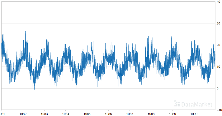
Minimum Daily Temperatures
The dataset shows a strong seasonality component and has a nice, fine-grained detail to work with.
Load the Minimum Daily Temperatures Dataset
Download the Minimum Daily Temperatures dataset and place it in the current working directory with the filename “daily-minimum-temperatures.csv“.
The code below will load and plot the dataset.
|
1 2 3 4 5 |
from pandas import read_csv from matplotlib import pyplot series = read_csv('daily-minimum-temperatures.csv', header=0, index_col=0) series.plot() pyplot.show() |
Running the example creates the following plot of the dataset.
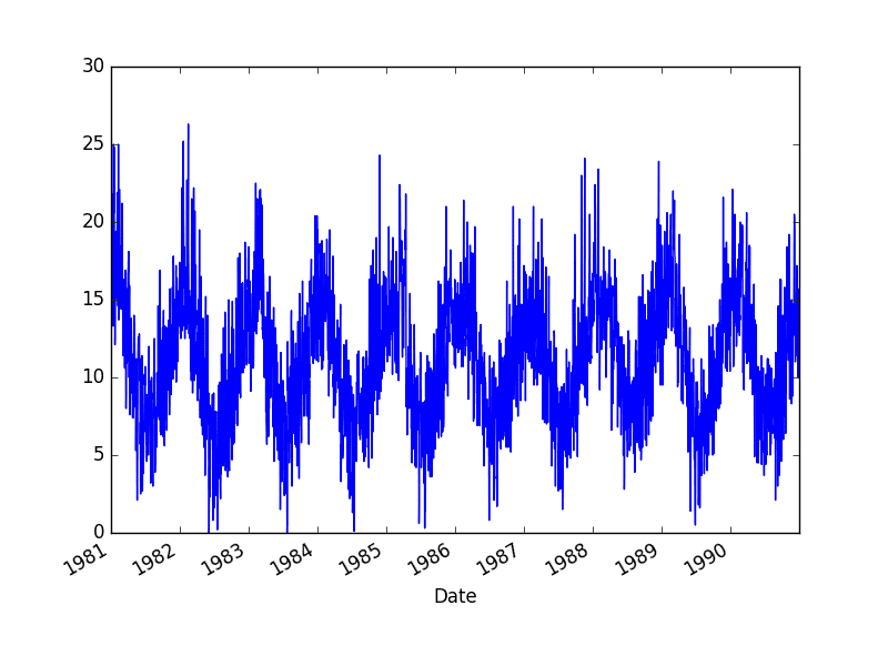
Minimum Daily Temperature Dataset
Seasonal Adjustment with Differencing
A simple way to correct for a seasonal component is to use differencing.
If there is a seasonal component at the level of one week, then we can remove it on an observation today by subtracting the value from last week.
In the case of the Minimum Daily Temperatures dataset, it looks like we have a seasonal component each year showing swing from summer to winter.
We can subtract the daily minimum temperature from the same day last year to correct for seasonality. This would require special handling of February 29th in leap years and would mean that the first year of data would not be available for modeling.
Below is an example of using the difference method on the daily data in Python.
|
1 2 3 4 5 6 7 8 9 10 11 |
from pandas import read_csv from matplotlib import pyplot series = read_csv('daily-minimum-temperatures.csv', header=0, index_col=0) X = series.values diff = list() days_in_year = 365 for i in range(days_in_year, len(X)): value = X[i] - X[i - days_in_year] diff.append(value) pyplot.plot(diff) pyplot.show() |
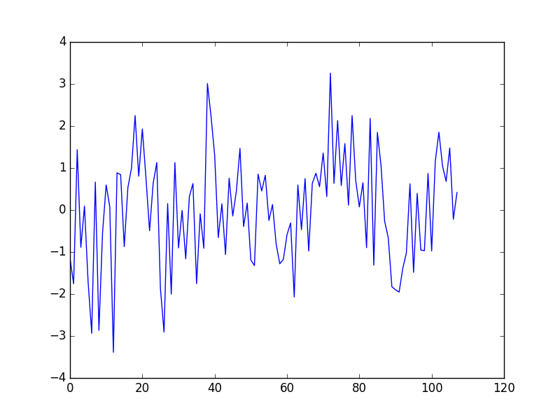
Running this example creates a new seasonally adjusted dataset and plots the result.
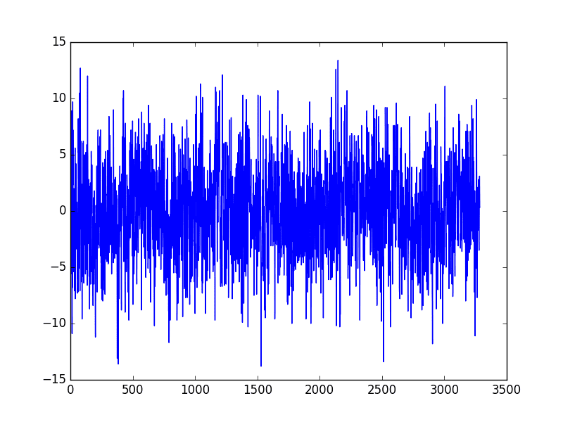
Differencing Sesaonal Adjusted Minimum Daily Temperature
There are two leap years in our dataset (1984 and 1988). They are not explicitly handled; this means that observations in March 1984 onwards the offset are wrong by one day, and after March 1988, the offsets are wrong by two days.
One option is to update the code example to be leap-day aware.
Another option is to consider that the temperature within any given period of the year is probably stable. Perhaps over a few weeks. We can shortcut this idea and consider all temperatures within a calendar month to be stable.
An improved model may be to subtract the average temperature from the same calendar month in the previous year, rather than the same day.
We can start off by resampling the dataset to a monthly average minimum temperature.
|
1 2 3 4 5 6 7 8 |
from pandas import read_csv from matplotlib import pyplot series = read_csv('daily-minimum-temperatures.csv', header=0, index_col=0) resample = series.resample('M') monthly_mean = resample.mean() print(monthly_mean.head(13)) monthly_mean.plot() pyplot.show() |
Running this example prints the first 13 months of average monthly minimum temperatures.
|
1 2 3 4 5 6 7 8 9 10 11 12 13 14 |
Date 1981-01-31 17.712903 1981-02-28 17.678571 1981-03-31 13.500000 1981-04-30 12.356667 1981-05-31 9.490323 1981-06-30 7.306667 1981-07-31 7.577419 1981-08-31 7.238710 1981-09-30 10.143333 1981-10-31 10.087097 1981-11-30 11.890000 1981-12-31 13.680645 1982-01-31 16.567742 |
It also plots the monthly data, clearly showing the seasonality of the dataset.
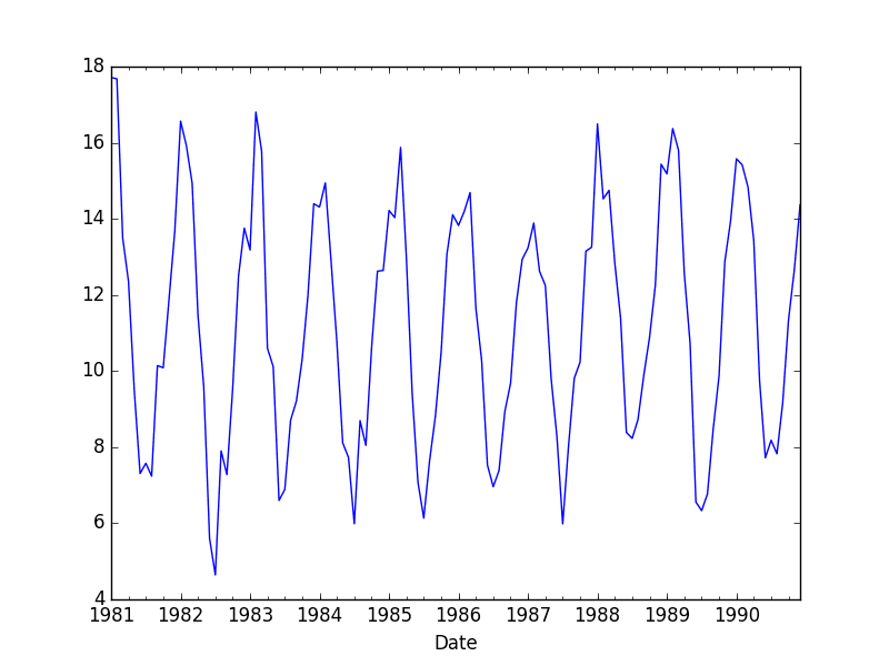
Minimum Monthly Temperature Dataset
We can test the same differencing method on the monthly data and confirm that the seasonally adjusted dataset does indeed remove the yearly cycles.
|
1 2 3 4 5 6 7 8 9 10 11 12 13 |
from pandas import read_csv from matplotlib import pyplot series = read_csv('daily-minimum-temperatures.csv', header=0, index_col=0) resample = series.resample('M') monthly_mean = resample.mean() X = series.values diff = list() months_in_year = 12 for i in range(months_in_year, len(monthly_mean)): value = monthly_mean[i] - monthly_mean[i - months_in_year] diff.append(value) pyplot.plot(diff) pyplot.show() |
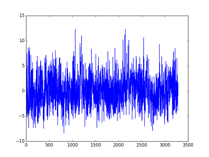
Running the example creates a new seasonally adjusted monthly minimum temperature dataset, skipping the first year of data in order to create the adjustment. The adjusted dataset is then plotted.
Seasonally Adjusted Minimum Monthly Temperature Dataset
Next, we can use the monthly average minimum temperatures from the same month in the previous year to adjust the daily minimum temperature dataset.
Again, we just skip the first year of data, but the correction using the monthly rather than the daily data may be a more stable approach.
|
1 2 3 4 5 6 7 8 9 10 11 12 13 |
from pandas import read_csv from matplotlib import pyplot series = read_csv('daily-minimum-temperatures.csv', header=0, index_col=0) X = series.values diff = list() days_in_year = 365 for i in range(days_in_year, len(X)): month_str = str(series.index[i].year-1)+'-'+str(series.index[i].month) month_mean_last_year = series[month_str].mean() value = X[i] - month_mean_last_year diff.append(value) pyplot.plot(diff) pyplot.show() |
Running the example again creates the seasonally adjusted dataset and plots the results.
This example is robust to daily fluctuations in the previous year and to offset errors creeping in due to February 29 days in leap years.
More Stable Seasonally Adjusted Minimum Monthly Temperature Dataset
The edge of calendar months provides a hard boundary that may not make sense for temperature data.
More flexible approaches that take the average from one week either side of the same date in the previous year may again be a better approach.
Additionally, there is likely to be seasonality in temperature data at multiple scales that may be corrected for directly or indirectly, such as:
- Day level.
- Multiple day level, such as a week or weeks.
- Multiple week level, such as a month.
- Multiple month level, such as a quarter or season.
Seasonal Adjustment with Modeling
We can model the seasonal component directly, then subtract it from the observations.
The seasonal component in a given time series is likely a sine wave over a generally fixed period and amplitude. This can be approximated easily using a curve-fitting method.
A dataset can be constructed with the time index of the sine wave as an input, or x-axis, and the observation as the output, or y-axis.
For example:
|
1 2 3 4 5 6 |
Time Index, Observation 1, obs1 2, obs2 3, obs3 4, obs4 5, obs5 |
Once fit, the model can then be used to calculate a seasonal component for any time index.
In the case of the temperature data, the time index would be the day of the year. We can then estimate the seasonal component for the day of the year for any historical observations or any new observations in the future.
The curve can then be used as a new input for modeling with supervised learning algorithms, or subtracted from observations to create a seasonally adjusted series.
Let’s start off by fitting a curve to the Minimum Daily Temperatures dataset. The NumPy library provides the polyfit() function that can be used to fit a polynomial of a chosen order to a dataset.
First, we can create a dataset of time index (day in this case) to observation. We could take a single year of data or all the years. Ideally, we would try both and see which model resulted in a better fit. We could also smooth the observations using a moving average centered on each value. This too may result in a model with a better fit.
Once the dataset is prepared, we can create the fit by calling the polyfit() function passing the x-axis values (integer day of year), y-axis values (temperature observations), and the order of the polynomial. The order controls the number of terms, and in turn the complexity of the curve used to fit the data.
Ideally, we want the simplest curve that describes the seasonality of the dataset. For consistent sine wave-like seasonality, a 4th order or 5th order polynomial will be sufficient.
In this case, I chose an order of 4 by trial and error. The resulting model takes the form:
|
1 |
y = x^4*b1 + x^3*b2 + x^2*b3 + x^1*b4 + b5 |
Where y is the fit value, x is the time index (day of the year), and b1 to b5 are the coefficients found by the curve-fitting optimization algorithm.
Once fit, we will have a set of coefficients that represent our model. We can then use this model to calculate the curve for one observation, one year of observations, or the entire dataset.
The complete example is listed below.
|
1 2 3 4 5 6 7 8 9 10 11 12 13 14 15 16 17 18 19 20 21 |
from pandas import read_csv from matplotlib import pyplot from numpy import polyfit series = read_csv('daily-minimum-temperatures.csv', header=0, index_col=0) # fit polynomial: x^2*b1 + x*b2 + ... + bn X = [i%365 for i in range(0, len(series))] y = series.values degree = 4 coef = polyfit(X, y, degree) print('Coefficients: %s' % coef) # create curve curve = list() for i in range(len(X)): value = coef[-1] for d in range(degree): value += X[i]**(degree-d) * coef[d] curve.append(value) # plot curve over original data pyplot.plot(series.values) pyplot.plot(curve, color='red', linewidth=3) pyplot.show() |
Running the example creates the dataset, fits the curve, predicts the value for each day in the dataset, and then plots the resulting seasonal model (red) over the top of the original dataset (blue).
One limitation of this model is that it does not take into account of leap days, adding small offset noise that could easily be corrected with an update to the approach.
For example, we could just remove the two February 29 observations from the dataset when creating the seasonal model.
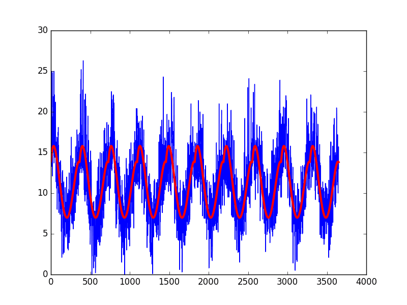
Curve Fit Seasonal Model of Daily Minimum Temperature
The curve appears to be a good fit for the seasonal structure in the dataset.
We can now use this model to create a seasonally adjusted version of the dataset.
The complete example is listed below.
|
1 2 3 4 5 6 7 8 9 10 11 12 13 14 15 16 17 18 19 20 21 22 23 24 25 |
from pandas import read_csv from matplotlib import pyplot from numpy import polyfit series = read_csv('daily-minimum-temperatures.csv', header=0, index_col=0) # fit polynomial: x^2*b1 + x*b2 + ... + bn X = [i%365 for i in range(0, len(series))] y = series.values degree = 4 coef = polyfit(X, y, degree) print('Coefficients: %s' % coef) # create curve curve = list() for i in range(len(X)): value = coef[-1] for d in range(degree): value += X[i]**(degree-d) * coef[d] curve.append(value) # create seasonally adjusted values = series.values diff = list() for i in range(len(values)): value = values[i] - curve[i] diff.append(value) pyplot.plot(diff) pyplot.show() |
Running the example subtracts the values predicted by the seasonal model from the original observations. The
The seasonally adjusted dataset is then plotted.
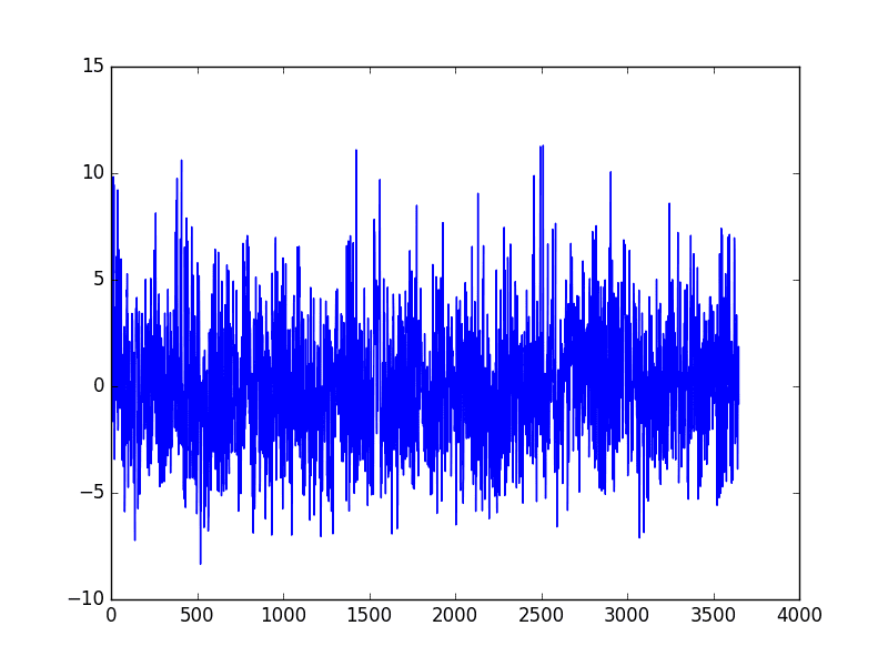
Curve Fit Seasonally Adjusted Daily Minimum Temperature
Summary
In this tutorial, you discovered how to create seasonally adjusted time series datasets in Python.
Specifically, you learned:
- The importance of seasonality in time series and the opportunities for data preparation and feature engineering it provides.
- How to use the difference method to create a seasonally adjusted time series.
- How to model the seasonal component directly and subtract it from observations.
Do you have any questions about deseasonalizing time series, or about this post?
Ask your questions in the comments below and I will do my best to answer.
Want to Develop Time Series Forecasts with Python?

Develop Your Own Forecasts in Minutes
...with just a few lines of python codeDiscover how in my new Ebook:
Introduction to Time Series Forecasting With Python
It covers self-study tutorials and end-to-end projects on topics like: Loading data, visualization, modeling, algorithm tuning, and much more...
Finally Bring Time Series Forecasting to
Your Own Projects
Skip the Academics. Just Results.


Is it right that after substracting sine which represents year cycle impact we’ve got values of deviation of daily temperature from its average? I just trying to understand what this result values mean. like your posts!
That is correct.
These first order difference values can then be used to fit a model. The model can then be used to make predictions, and the seasonal component added back to the prediction for a final usable value.
Does that help?
Definitely! Thanks. I think another possible method for feature engineering would be using empirical mode decomposition algorythm to extract different signal components to be used in fitting model, will test it.
Can you be more specific how to add the seasonal component back..? I couldn’t see how to preserve this seasonal component during deseasonalizing… Or I missed something… if so, please indicate where it is. Thank you…!
If you seasonally adjust by subtracting data from 1 year ago, you can reverse it by adding the subtracted value back again.
By the way there is a usefull library for EMD on github: https://github.com/jaidevd/pyhht
Thanks for the link augmentale.
I have seen where people use decomposition and take error/residual part to remove trend and seasonality. How to choose which method/technique to use to remove seasonality/trend?
Hi Amit,
Decomposition is good for time series analysis, but generally unusable for time series forecasting. At least as I understand it.
I would suggest trying a suite of methods and see what works best – results in models with the most accurate forecasts.
how to deseasonalize time series when some of the data have seasonal effect and others does nit
Prepare each series separatly.
Hi Jason,
I have to predict 3 day household electricity demand @ 12 hour interval for next 3 days (6 data points). I have ~ 3 years of data at 12 hours interval. On face of it, it looks as if there could be multiple seasonal patterns.How can I identify complex seasonal periods?What could be the best approach in that case?
Sounds fun.
Try fitting some polynomials perhaps?
Hi,
I have a data which has multiple seasonalities .is there any way to identify all the seasonalities.I have tried sesonal decompose but we need to pass the parameter for Monthly, weekly or yearly My case we I need to identify all the seasonalities occurs in my data .
Thanks in advance.
Regards,
BMK
Perhaps look at a graph and use seasonal differencing to remove each in turn.
Hey, you may use a fourier transform to find the season frequencies. Good Luck!
Great suggestion.
I cannot see the benefits from deseasonalization if i want to predict certain value. Im missing this information if i do it.
The model for the seasonality is easy, so we model it and remove it. Then, we want to add more value on top of that.
if i have a seasonal time series and its general trend. Can it be AR,MA,ARMA or ARIMA and if I can show you th data plz. Thanks
Sorry, I don’t understand your question. Perhaps you can restate it?
How to check seasonality semi annual variation in data???
Kindly describe briefly.
Thanks
What do you mean exactly?
Hi Jason. Great post! So easy to follow 🙂
I’m pretty new to python so excuse the basic-ness of this question. How do you ‘keep’ the seasonally adjusted values. Such as write to ascii or some other technique, so that I am able to use this data in other scripts. Many thanks
Good question, you can save the data to a CSV file.
This post has a few options you can try:
https://stackoverflow.com/questions/6081008/dump-a-numpy-array-into-a-csv-file
can we use this technique to compare signals with different lengths? For eg. Signal A is recorded for 5 sec, signal B is recorded for 1 min. If we want to compare these 2 signals, can I use your idea to remove the seasonal components of the longest signal?
Sorry, I’m not sure I follow. Perhaps try it and see.
Great post. Thank you very much Jason. I also followed your ARIMA post and wondering if ARIMA can handle it all (including seasonality) so we don’t necessarily have to isolate out and handle seasonality and do ARIMA on the seasonality-adjusted data. Because technically seasonality is a special form of auto-correlation and can be handled by differencing. am I thinking correctly?
Your models will perform better if you remove systematic patterns from the data such as trends and seasonality.
Thanks very much for this post Jason! I need to analyze extreme values in a climate dataset that has very strong seasonality – this recipe is EXACTLY what I need achieve that task 🙂
People like you who take the time to post methods & examples like this make life a heck of a lot easier (and less frustrating!) for people like me who need to extract valuable information from datasets using techniques that we aren’t necessarily trained in. And consequently, you make the world a better place for us!
Thanks again
I’m glad I could help Ian!
how can I use this for weekly and annually seasonality?
You will need to modify it accordingly.
Why cycle is usually ignored in time series modelling?
Seasonality is a cycle, and it is not ignored. We can remove it or model it with an SARIMA model:
https://machinelearningmastery.com/how-to-grid-search-sarima-model-hyperparameters-for-time-series-forecasting-in-python/
multiple seasonality in same data series?
This is a great example – thank you.
The examples are quite mechanical – thus good for general audience.
Just wondering if/why_not considered using pandas.groupby and .transform methods?
Thanks Edward.
How do you think I should use those methods in the above tutorial?
Hello Jason,
This is a great post thanks.
I have some queries.
1) Is it already neccessary to remove the trend and/or seasonality from the timeseries data before applying the SARIMAX (seasonal arima) model?
2) How can I statistically know whether the timeseries data is stationary or not? That is using adf.test and if the p-value>0.05 can I assume the data is not stationary?
3) Last one; is it neccessary to make the data stationary if any other models are used like HoltsWinter or Exponential Smoothing etc?
Please advise.
It can help to remove structure like trends and seasonality. The problem will be simpler and model skill higher. But it is not required to perform these operations.
This post has info on testing the stationarity:
https://machinelearningmastery.com/time-series-data-stationary-python/
Again, the series does not have to be stationary, but most methods assume it and in turn model skill will often be higher if you meet the assumption.
Hi,
Do we need remove seasonality before performing deep learning methods, like MLP or LSTM?
Thanks in advance.
Anything we can do to make the problem simpler for the model is a good idea.
Hi,
I coppied the code from the first window straight into jupyter notebook running on Ubuntu and I get 2 errors.
1. relating to the use of from_csv being depreciated
2. I also get an indexing error.
—————————————————————————
IndexError Traceback (most recent call last)
in ()
1 from pandas import Series
2 from matplotlib import pyplot
—-> 3 series = Series.from_csv(‘daily-minimum-temperatures.csv’, header=0)
4 series.plot()
5 pyplot.show()
~/anaconda3/lib/python3.6/site-packages/pandas/core/series.py in from_csv(cls, path, sep, parse_dates, header, index_col, encoding, infer_datetime_format)
2888 sep=sep, parse_dates=parse_dates,
2889 encoding=encoding,
-> 2890 infer_datetime_format=infer_datetime_format)
2891 result = df.iloc[:, 0]
2892 if header is None:
.
.
.
.
IndexError: list index out of range
I’m sorry to hear that, try these steps:
https://machinelearningmastery.com/faq/single-faq/why-does-the-code-in-the-tutorial-not-work-for-me
Hi, I was wondering if you can suggest any method to predict the start date of the seasonality. For example, the start date of summer or winter.
Thank you
It really depends what ‘start’ means for your problem. You must define start, then you can predict it.
Hi,
How would I define the weekly seasonality in my model using Minitab? Is it define as S=4?
Thanks in advance.
What is “minitab”?
Hi Jason,
Thanks a lot for the post!
“For time series with a seasonal component, the lag may be expected to be the period (width) of the seasonality.”
I have a seasonality from Aug to Feb each year. Eg.
2016-08 12.84M
2016-09 21.43M
2016-10 24.74M
2016-11 21.46M
2016-12 20.21M
2017-01 16.75M
2017-02 13.46M
M = in Millions
Do I need to consider the lag as 6 or 7 ? Please suggest.
Also, on top of the differentiated data set we need to perorfm trend removal, then Feed it to the ARIMA model?
Kindly confirm. Thanks a lot. 🙂
Sorry, I cannot analyse the seasonality of your data for you.
Hi Jason,
What if the “seasonal” component is not fixed, that is, the length of each cycle changes? An example of this is the sunspot number, which is not exactly 11 years, but changes from cycle to cycle. How to remove the cyclic component then?
Great question, time series gets tricky.
I believe the seasonal component can be modelled with the expectation of change, perhaps check out exponential smoothing:
https://machinelearningmastery.com/how-to-grid-search-triple-exponential-smoothing-for-time-series-forecasting-in-python/
Hi,
Is there a way to model Free disk_space,Cpu usage,network&infrastructure monitoring please let me know the resources
Sure, perhaps start here:
https://machinelearningmastery.com/start-here/#process
Thanks for your post !
It is awesome post I’ve ever seen 🙂
May I ask you quick question?
I am confused with deterministic trend/seasonality and stochastic trend/seasonality.
Here is my question:
It is ok to get rid of deterministic trend/seasonality first and then proceed multiplicative SARIMAX modeling process?
I am not sure data can have both of deterministic & stochastic trend/seasonality at the same time.
Thanks.
Thanks.
You’re approach sounds sensible.
Hello Jason, thank you very much for your post.
I am trying to use you approach on a different type of problem, however I have some doubts I’ve not been able to solve yet.
Would this approach be convenient for a “consumer consuption” seasonality type of analysis. That is, to understand how consumers behave along the year (on a monthly basis). And if so, how can the model make up for changes along the years, for example new stores being opened along the years being analyzed (creating a spike in sales on the analyzed data). Would it be more convenient to take away the entry of these new stores being opened?
Thanks in advance!
Perhaps try it and see if it is appropriate.
It might be easier to use a model that can better capture the seasonality, e.g. SARIMA or ETS.
Great article!
Two questions-
Why do we need to remove seasonality before applying ARIMA if we are anyway going to provide the value of ‘d’ in ARIMA (p,d,q)?
Why do we need SARIMA if we are already having ARIMA, where we can give a value of, ‘d’ to handle seasonality?
Thanks.
Good questions.
Differencing will make it stationary, removing the seasonality explicitly will also make it stationary. It’s a choice and more control might be preferred.
Modeling the seasonality can improve model performance.
Thanks for the response, Jason.
I came across some an example on Otexts chapter 12.8. (Hopefully, you are aware of otexts)
The statement goes like this –
cafe<-Arima(training, order=c(2,1,1), seasonal=c(0,1,2), lambda=0)
Now, this is confusing me a lot. Here the value of d =1 is provided which means seasonality has been removed and the series is stationary now but then again the seasonal component is provided with D = 1.
Could you please explain to me what is happening here?
I have an interview for a job and I am stuck with this topic related to seasonality in Arima.
Thank you again for your time.
Here the first d is removing the trend (trend adjustment), the second is D removing the seasonality (seasonal adjustment).
Does that help?
Yes, it does. Thanks a lot, Jason.
Hi Jason,
do I need deseasonalization for LSTMs? It seems like there is no consensus about that in the literature.
It can be very helpful! E.g. it makes the problem simpler to model.
There is an error in the code where you decomposed the time series in based on monthly mean. “x = series.values” should be “monthly_mean = monthly_mean.values”. Please correct me if I m wrong.
I don’t believe so.
Take a look at the fourth code snipet. Whats the point below for the line: X = series.values? you are not using X in the code. Morever, monthly mean can not be accessed via monthly_mean[i] when monthly_mean = resample.mean();
from pandas import read_csv
from matplotlib import pyplot
series = read_csv(‘daily-minimum-temperatures.csv’, header=0, index_col=0)
resample = series.resample(‘M’)
monthly_mean = resample.mean()
X = series.values
diff = list()
months_in_year = 12
for i in range(months_in_year, len(monthly_mean)):
value = monthly_mean[i] – monthly_mean[i – months_in_year]
diff.append(value)
pyplot.plot(diff)
pyplot.show()
Yes, you can ignore it.
You can access monthly_mean by this way
value = monthly_mean.iloc[i][‘Temp’] – monthly_mean.iloc[i – months_in_year][‘Temp’]
I need to infer the seasonality from the given timeseries. My intention is to find out at which time frame the given series is meeting the given threshold.
For example, out of the given CPU percentage series for 1 month with 1 hour granularity. I need to get statements like
Every day at 3rd hour and 7th hour it is meeting threshold.
Every week on Sunday 5 and 8th hour threshold met.
Alternative day, 16th hour threshold is met.
Perhaps try it and see?
I am trying to Trend analysis of daily and monthly rainfall data using Kendall package in R software. But I am getting this error everytime I try to the MannKendall analysis.
> MannKendall(data)
Error in Kendall(1:length(x), x) : length(x)<3
Can you please help me in solving this error if possible??
Sorry, I am not familiar with that package, perhaps try posting to cross validated?
Hi,
I am working on methane emission data from the past 30 years. I want to know if climate change has had an effect on the variance/width/amplitude of the seasonality in my methane data. How could I quantify this?
Perhaps look into causal models?
Perhaps look into statistical correlation for time series data?
Pretty sure there is a bug in the loop of Curve Fit Seasonal Model of Daily Minimum Temperature.
Plots come out all wrong for me.
Replacing the loop with polyval(coef, X) solves the problem (note polyval needs to be imported from numpy)
Are you sure, did you copy all code as-is? Run from the command line?
More here:
https://machinelearningmastery.com/faq/single-faq/why-does-the-code-in-the-tutorial-not-work-for-me
A whole day fighting with a lot of numpy and strange array & list conversions, only to find this solution! Jason, Brett solution made my day!
This tutorial is very helpful !
Can you please guide me about, what are the benefits of Seasonal Adjustment / Deseasonalizing the time series data?
It removes a simple structure from the series so the model can focus on learning the more complex structures.
Is there any way to detect stationarity , seasonality and noise in data without plotting graph. Please let me know
Probably, I have not seen reliable methods.
Hey Jason, I am trying to make a forecast by using 4 years of daily data which is about grocery sales. When I look the decomposition graphs I observe negligible trend and in order to look for seasonality I transformed my data to weekly and observed seasonal patterns.
1) I used my daily data for forecasting, firstly I checked out adf test and results seems okey, so in order to catch the seasonality I used SARIMA model for forecasting is it an acceptable approach ?
2)I will going to make forecasting using Random Forest and other tree methods and also LSTM, should I remove my seasonality before fitting models and revert back to it to my prediction ? or using simply adding another feature which is rolling mean with window 7 days ?
3) Lastly, before making any differencing/deseasonaling I should divide my sample to train and test right ? Could I make such kind of operations to the all sample ?
Nice work.
Yes, SARIMA is a good start. Also perhaps test ETS.
Yes, try ML models on the raw data then try removing seasonality and compare the results.
You can divide into train/test after differencing, it rarely results in data leakage.
Hi Jason,
Really great presentation especially the modeling approach.
Have you tried before the FFT approach for seasonality removing too? If so, please include the link.
Examples on the internet are not so clear and strong as your works!
I don’t have tutorial on that topic at this stage.
Hi, Jason!
I just copied the code from the “modeling” chapter and the results are completely different from the results in the article. what could cause it?
The book may be more up to date than the blog.
Also, see this:
https://machinelearningmastery.com/ufaqs/why-do-i-get-different-results-each-time-i-run-the-code/
I learned a lot from this post, thanks Jason
But I have a question If our seasonal data adjusted by differencing we just need to reverse it by adding the subtracted value back again to get the original value.
What we should do to get the original predicted value again if we adjusted the seasonal data with modeling? Because we don’t have the curve value in t+1, only the predicted value (yhat).
You add the value from one cycle ago in the input data or training data.
Hi Jason,
Thank you for your post.
I read it, also read a post titled (How to Check if Time Series Data is Stationary with Python). Then I applied the same dataset to check the stationary using the ‘Augmented Dickey-Fuller test’. The result shows the time series is stationary. Why did that happen? Because I have a similar dataset, also my result shows the time series is stationary but I know it’s seasonality from the line plot.
Thank you.
Stationary time series can also be seasonal. A sine wave, for example, is stationary.
Nice post, really good. I’m applying thar seasonal difference after a simple difference, do you have any clue how I can reverse it ? My data is a monthly data. Thanks a lot.
You mean how to reverse a difference? That operation is called a cumulative sum (cumsum() function).
I can reverse the seasonal difference with cumsum() ?
cumsum() is adding adjacent numbers in a sequence. If you can somehow present seasonal data in a sequence (e.g., resample the data), then it should work.
hi Adrian Tam
I have a weather time-series dataset of two years, I want to use the same method to remove seasonality, but the first year will be assigned as Null values, and I need these values because one year is not enough for my model to make a prediction, so is there another method that keeps the values of the first year?
See if this helps: https://machinelearningmastery.com/sarima-for-time-series-forecasting-in-python/
How do I de-seasonalize a new test data point? Like I were to deploy time series model trained on de-seasonlized data how can I use to forecast on new future test data point?
Hi Soumitra…For time-series forecasting applications you will always have the data up to the point at which you will start making predictions. Thus, you will be able to remove seasonality as discussed in the tutorial.
Hello, Jason
I’m using a LSTM model for series prediction. Some of my input series have both linear trend and seasonality.
I was thinking about removing the linear trend first and then the seasonality.
My question is the following, should I do that before splitting in training and test sets? If the answer if yes, how should I treat the new data on which I want to make predictions? I mean, what trend and seasonality should I remove from this new data?
Thank you so much in advance!
Hello Jason,
I am an Astronomer, I am on a project. In that project, I have a time series data. To check the stationarity of time series, I have done some test like “Augmented Dickey Fuller” and ” KPSS” test and I found that my time series is stationary. Now I want to check seasonality component in time series, which I can not do by visual inspection. for that I need rely on some other method. So to do that, I have generated all possible combination of order parameters of models (p,d,q)*(P,D,Q,S), where (p,q,d stand for order parameter of non-seasonal AR, MA model and non-seasonal differencing respectively and P,Q,D,S are representing the seasonal AR, MA models, seasonal differencing and seasonality component), have fitted with “SARIMAX” model, have tried to determine the lowest AIC value. As we know lowest AIC value represent best optimal model for our time series. When I did that, I found at lowest AIC value, I got order parameters for example (1,1,1)*(2,0,0,58). there should not differencing parameter=1 in non-seasonal component. Why I am getting this type result, Could you please explain?
Hi Ajay…You may wish to investigate LSTM models for your application:
https://machinelearningmastery.com/multivariate-time-series-forecasting-lstms-keras/