Data cleaning is a critically important step in any machine learning project.
In tabular data, there are many different statistical analysis and data visualization techniques you can use to explore your data in order to identify data cleaning operations you may want to perform.
Before jumping to the sophisticated methods, there are some very basic data cleaning operations that you probably should perform on every single machine learning project. These are so basic that they are often overlooked by seasoned machine learning practitioners, yet are so critical that if skipped, models may break or report overly optimistic performance results.
In this tutorial, you will discover basic data cleaning you should always perform on your dataset.
After completing this tutorial, you will know:
- How to identify and remove column variables that only have a single value.
- How to identify and consider column variables with very few unique values.
- How to identify and remove rows that contain duplicate observations.
Kick-start your project with my new book Data Preparation for Machine Learning, including step-by-step tutorials and the Python source code files for all examples.
Let’s get started.
- Updated Apr/2020: Added a section on Datasets and the VarianceThreshold.
- Updated May/2020: Added quotes and book references.

Basic Data Cleaning You Must Perform in Machine Learning
Photo by Allen McGregor, some rights reserved.
Tutorial Overview
This tutorial is divided into seven parts; they are:
- Messy Datasets
- Identify Columns That Contain a Single Value
- Delete Columns That Contain a Single Value
- Consider Columns That Have Very Few Values
- Remove Columns That Have A Low Variance
- Identify Rows that Contain Duplicate Data
- Delete Rows that Contain Duplicate Data
Messy Datasets
Data cleaning refers to identifying and correcting errors in the dataset that may negatively impact a predictive model.
Data cleaning is used to refer to all kinds of tasks and activities to detect and repair errors in the data.
— Page xiii, Data Cleaning, 2019.
Although critically important, data cleaning is not exciting, not does it involve fancy techniques. Just a good knowledge of the dataset.
Cleaning up your data is not the most glamourous of tasks, but it’s an essential part of data wrangling. […] Knowing how to properly clean and assemble your data will set you miles apart from others in your field.
— Page 149, Data Wrangling with Python, 2016.
There are many types of errors that exist in a dataset, although some of the simplest errors include columns that don’t contain much information and duplicated rows.
Before we dive into identifying and correcting messy data, let’s define some messy datasets.
We will use two datasets as the basis for this tutorial, the oil spill dataset and the iris flowers dataset.
Want to Get Started With Data Preparation?
Take my free 7-day email crash course now (with sample code).
Click to sign-up and also get a free PDF Ebook version of the course.
Oil Spill Dataset
The so-called “oil spill” dataset is a standard machine learning dataset.
The task involves predicting whether the patch contains an oil spill or not, e.g. from the illegal or accidental dumping of oil in the ocean, given a vector that describes the contents of a patch of a satellite image.
There are 937 cases. Each case is comprised of 48 numerical computer vision derived features, a patch number, and a class label.
The normal case is no oil spill assigned the class label of 0, whereas an oil spill is indicated by a class label of 1. There are 896 cases for no oil spill and 41 cases of an oil spill.
You can access the entire dataset here:
Review the contents of the file.
The first few lines of the file should look as follows:
|
1 2 3 4 5 6 |
1,2558,1506.09,456.63,90,6395000,40.88,7.89,29780,0.19,214.7,0.21,0.26,0.49,0.1,0.4,99.59,32.19,1.84,0.16,0.2,87.65,0,0.47,132.78,-0.01,3.78,0.22,3.2,-3.71,-0.18,2.19,0,2.19,310,16110,0,138.68,89,69,2850,1000,763.16,135.46,3.73,0,33243.19,65.74,7.95,1 2,22325,79.11,841.03,180,55812500,51.11,1.21,61900,0.02,901.7,0.02,0.03,0.11,0.01,0.11,6058.23,4061.15,2.3,0.02,0.02,87.65,0,0.58,132.78,-0.01,3.78,0.84,7.09,-2.21,0,0,0,0,704,40140,0,68.65,89,69,5750,11500,9593.48,1648.8,0.6,0,51572.04,65.73,6.26,0 3,115,1449.85,608.43,88,287500,40.42,7.34,3340,0.18,86.1,0.21,0.32,0.5,0.17,0.34,71.2,16.73,1.82,0.19,0.29,87.65,0,0.46,132.78,-0.01,3.78,0.7,4.79,-3.36,-0.23,1.95,0,1.95,29,1530,0.01,38.8,89,69,1400,250,150,45.13,9.33,1,31692.84,65.81,7.84,1 4,1201,1562.53,295.65,66,3002500,42.4,7.97,18030,0.19,166.5,0.21,0.26,0.48,0.1,0.38,120.22,33.47,1.91,0.16,0.21,87.65,0,0.48,132.78,-0.01,3.78,0.84,6.78,-3.54,-0.33,2.2,0,2.2,183,10080,0,108.27,89,69,6041.52,761.58,453.21,144.97,13.33,1,37696.21,65.67,8.07,1 5,312,950.27,440.86,37,780000,41.43,7.03,3350,0.17,232.8,0.15,0.19,0.35,0.09,0.26,289.19,48.68,1.86,0.13,0.16,87.65,0,0.47,132.78,-0.01,3.78,0.02,2.28,-3.44,-0.44,2.19,0,2.19,45,2340,0,14.39,89,69,1320.04,710.63,512.54,109.16,2.58,0,29038.17,65.66,7.35,0 ... |
We can see that the first column contains integers for the patch number. We can also see that the computer vision derived features are real-valued with differing scales such as thousands in the second column and fractions in other columns.
This dataset contains columns with very few unique values that provides a good basis for data cleaning.
Iris Flowers Dataset
The so-called “iris flowers” dataset is another standard machine learning dataset.
The dataset involves predicting the flower species given measurements of iris flowers in centimeters.
It is a multi-class classification problem. The number of observations for each class is balanced. There are 150 observations with 4 input variables and 1 output variable.
You can access the entire dataset here:
Review the contents of the file.
The first few lines of the file should look as follows:
|
1 2 3 4 5 6 |
5.1,3.5,1.4,0.2,Iris-setosa 4.9,3.0,1.4,0.2,Iris-setosa 4.7,3.2,1.3,0.2,Iris-setosa 4.6,3.1,1.5,0.2,Iris-setosa 5.0,3.6,1.4,0.2,Iris-setosa ... |
We can see that all four input variables are numeric and that the target class variable is a string representing the iris flower species.
This dataset contains duplicate rows that provides a good basis for data cleaning.
Identify Columns That Contain a Single Value
Columns that have a single observation or value are probably useless for modeling.
These columns or predictors are referred to zero-variance predictors as if we measured the variance (average value from the mean), it would be zero.
When a predictor contains a single value, we call this a zero-variance predictor because there truly is no variation displayed by the predictor.
— Page 96, Feature Engineering and Selection, 2019.
Here, a single value means that each row for that column has the same value. For example, the column X1 has the value 1.0 for all rows in the dataset:
|
1 2 3 4 5 6 7 |
X1 1.0 1.0 1.0 1.0 1.0 ... |
Columns that have a single value for all rows do not contain any information for modeling.
Depending on the choice of data preparation and modeling algorithms, variables with a single value can also cause errors or unexpected results.
You can detect rows that have this property using the unique() NumPy function that will report the number of unique values in each column.
The example below loads the oil-spill classification dataset that contains 50 variables and summarizes the number of unique values for each column.
|
1 2 3 4 5 6 7 8 9 10 11 |
# summarize the number of unique values for each column using numpy from urllib.request import urlopen from numpy import loadtxt from numpy import unique # define the location of the dataset path = 'https://raw.githubusercontent.com/jbrownlee/Datasets/master/oil-spill.csv' # load the dataset data = loadtxt(urlopen(path), delimiter=',') # summarize the number of unique values in each column for i in range(data.shape[1]): print(i, len(unique(data[:, i]))) |
Running the example loads the dataset directly from the URL and prints the number of unique values for each column.
We can see that column index 22 only has a single value and should be removed.
|
1 2 3 4 5 6 7 8 9 10 11 12 13 14 15 16 17 18 19 20 21 22 23 24 25 26 27 28 29 30 31 32 33 34 35 36 37 38 39 40 41 42 43 44 45 46 47 48 49 50 |
0 238 1 297 2 927 3 933 4 179 5 375 6 820 7 618 8 561 9 57 10 577 11 59 12 73 13 107 14 53 15 91 16 893 17 810 18 170 19 53 20 68 21 9 22 1 23 92 24 9 25 8 26 9 27 308 28 447 29 392 30 107 31 42 32 4 33 45 34 141 35 110 36 3 37 758 38 9 39 9 40 388 41 220 42 644 43 649 44 499 45 2 46 937 47 169 48 286 49 2 |
A simpler approach is to use the nunique() Pandas function that does the hard work for you.
Below is the same example using the Pandas function.
|
1 2 3 4 5 6 7 8 |
# summarize the number of unique values for each column using numpy from pandas import read_csv # define the location of the dataset path = 'https://raw.githubusercontent.com/jbrownlee/Datasets/master/oil-spill.csv' # load the dataset df = read_csv(path, header=None) # summarize the number of unique values in each column print(df.nunique()) |
Running the example, we get the same result, the column index, and the number of unique values for each column.
|
1 2 3 4 5 6 7 8 9 10 11 12 13 14 15 16 17 18 19 20 21 22 23 24 25 26 27 28 29 30 31 32 33 34 35 36 37 38 39 40 41 42 43 44 45 46 47 48 49 50 51 |
0 238 1 297 2 927 3 933 4 179 5 375 6 820 7 618 8 561 9 57 10 577 11 59 12 73 13 107 14 53 15 91 16 893 17 810 18 170 19 53 20 68 21 9 22 1 23 92 24 9 25 8 26 9 27 308 28 447 29 392 30 107 31 42 32 4 33 45 34 141 35 110 36 3 37 758 38 9 39 9 40 388 41 220 42 644 43 649 44 499 45 2 46 937 47 169 48 286 49 2 dtype: int64 |
Delete Columns That Contain a Single Value
Variables or columns that have a single value should probably be removed from your dataset.
… simply remove the zero-variance predictors.
— Page 96, Feature Engineering and Selection, 2019.
Columns are relatively easy to remove from a NumPy array or Pandas DataFrame.
One approach is to record all columns that have a single unique value, then delete them from the Pandas DataFrame by calling the drop() function.
The complete example is listed below.
|
1 2 3 4 5 6 7 8 9 10 11 12 13 14 15 |
# delete columns with a single unique value from pandas import read_csv # define the location of the dataset path = 'https://raw.githubusercontent.com/jbrownlee/Datasets/master/oil-spill.csv' # load the dataset df = read_csv(path, header=None) print(df.shape) # get number of unique values for each column counts = df.nunique() # record columns to delete to_del = [i for i,v in enumerate(counts) if v == 1] print(to_del) # drop useless columns df.drop(to_del, axis=1, inplace=True) print(df.shape) |
Running the example first loads the dataset and reports the number of rows and columns.
The number of unique values for each column is calculated, and those columns that have a single unique value are identified. In this case, column index 22.
The identified columns are then removed from the DataFrame, and the number of rows and columns in the DataFrame are reported to confirm the change.
|
1 2 3 |
(937, 50) [22] (937, 49) |
Consider Columns That Have Very Few Values
In the previous section, we saw that some columns in the example dataset had very few unique values.
For example, there were columns that only had 2, 4, and 9 unique values. This might make sense for ordinal or categorical variables. In this case, the dataset only contains numerical variables. As such, only having 2, 4, or 9 unique numerical values in a column might be surprising.
We can refer to these columns or predictors as near-zero variance predictors, as their variance is not zero, but a very small number close to zero.
… near-zero variance predictors or have the potential to have near zero variance during the resampling process. These are predictors that have few unique values (such as two values for binary dummy variables) and occur infrequently in the data.
— Pages 96-97, Feature Engineering and Selection, 2019.
These columns may or may not contribute to the skill of a model. We can’t assume that they are useless to modeling.
Although near-zero variance predictors likely contain little valuable predictive information, we may not desire to filter these out.
— Page 97, Feature Engineering and Selection, 2019.
Depending on the choice of data preparation and modeling algorithms, variables with very few numerical values can also cause errors or unexpected results. For example, I have seen them cause errors when using power transforms for data preparation and when fitting linear models that assume a “sensible” data probability distribution.
To help highlight columns of this type, you can calculate the number of unique values for each variable as a percentage of the total number of rows in the dataset.
Let’s do this manually using NumPy. The complete example is listed below.
|
1 2 3 4 5 6 7 8 9 10 11 12 13 |
# summarize the percentage of unique values for each column using numpy from urllib.request import urlopen from numpy import loadtxt from numpy import unique # define the location of the dataset path = 'https://raw.githubusercontent.com/jbrownlee/Datasets/master/oil-spill.csv' # load the dataset data = loadtxt(urlopen(path), delimiter=',') # summarize the number of unique values in each column for i in range(data.shape[1]): num = len(unique(data[:, i])) percentage = float(num) / data.shape[0] * 100 print('%d, %d, %.1f%%' % (i, num, percentage)) |
Running the example reports the column index and the number of unique values for each column, followed by the percentage of unique values out of all rows in the dataset.
Here, we can see that some columns have a very low percentage of unique values, such as below 1 percent.
|
1 2 3 4 5 6 7 8 9 10 11 12 13 14 15 16 17 18 19 20 21 22 23 24 25 26 27 28 29 30 31 32 33 34 35 36 37 38 39 40 41 42 43 44 45 46 47 48 49 50 |
0, 238, 25.4% 1, 297, 31.7% 2, 927, 98.9% 3, 933, 99.6% 4, 179, 19.1% 5, 375, 40.0% 6, 820, 87.5% 7, 618, 66.0% 8, 561, 59.9% 9, 57, 6.1% 10, 577, 61.6% 11, 59, 6.3% 12, 73, 7.8% 13, 107, 11.4% 14, 53, 5.7% 15, 91, 9.7% 16, 893, 95.3% 17, 810, 86.4% 18, 170, 18.1% 19, 53, 5.7% 20, 68, 7.3% 21, 9, 1.0% 22, 1, 0.1% 23, 92, 9.8% 24, 9, 1.0% 25, 8, 0.9% 26, 9, 1.0% 27, 308, 32.9% 28, 447, 47.7% 29, 392, 41.8% 30, 107, 11.4% 31, 42, 4.5% 32, 4, 0.4% 33, 45, 4.8% 34, 141, 15.0% 35, 110, 11.7% 36, 3, 0.3% 37, 758, 80.9% 38, 9, 1.0% 39, 9, 1.0% 40, 388, 41.4% 41, 220, 23.5% 42, 644, 68.7% 43, 649, 69.3% 44, 499, 53.3% 45, 2, 0.2% 46, 937, 100.0% 47, 169, 18.0% 48, 286, 30.5% 49, 2, 0.2% |
We can update the example to only summarize those variables that have unique values that are less than 1 percent of the number of rows.
|
1 2 3 4 5 6 7 8 9 10 11 12 13 14 |
# summarize the percentage of unique values for each column using numpy from urllib.request import urlopen from numpy import loadtxt from numpy import unique # define the location of the dataset path = 'https://raw.githubusercontent.com/jbrownlee/Datasets/master/oil-spill.csv' # load the dataset data = loadtxt(urlopen(path), delimiter=',') # summarize the number of unique values in each column for i in range(data.shape[1]): num = len(unique(data[:, i])) percentage = float(num) / data.shape[0] * 100 if percentage < 1: print('%d, %d, %.1f%%' % (i, num, percentage)) |
Running the example, we can see that 11 of the 50 variables have numerical variables that have unique values that are less than 1 percent of the number of rows.
This does not mean that these rows and columns should be deleted, but they require further attention.
For example:
- Perhaps the unique values can be encoded as ordinal values?
- Perhaps the unique values can be encoded as categorical values?
- Perhaps compare model skill with each variable removed from the dataset?
|
1 2 3 4 5 6 7 8 9 10 11 |
21, 9, 1.0% 22, 1, 0.1% 24, 9, 1.0% 25, 8, 0.9% 26, 9, 1.0% 32, 4, 0.4% 36, 3, 0.3% 38, 9, 1.0% 39, 9, 1.0% 45, 2, 0.2% 49, 2, 0.2% |
For example, if we wanted to delete all 11 columns with unique values less than 1 percent of rows; the example below demonstrates this.
|
1 2 3 4 5 6 7 8 9 10 11 12 13 14 15 |
# delete columns where number of unique values is less than 1% of the rows from pandas import read_csv # define the location of the dataset path = 'https://raw.githubusercontent.com/jbrownlee/Datasets/master/oil-spill.csv' # load the dataset df = read_csv(path, header=None) print(df.shape) # get number of unique values for each column counts = df.nunique() # record columns to delete to_del = [i for i,v in enumerate(counts) if (float(v)/df.shape[0]*100) < 1] print(to_del) # drop useless columns df.drop(to_del, axis=1, inplace=True) print(df.shape) |
Running the example first loads the dataset and reports the number of rows and columns.
The number of unique values for each column is calculated, and those columns that have a number of unique values less than 1 percent of the rows are identified. In this case, 11 columns.
The identified columns are then removed from the DataFrame, and the number of rows and columns in the DataFrame are reported to confirm the change.
|
1 2 3 |
(937, 50) [21, 22, 24, 25, 26, 32, 36, 38, 39, 45, 49] (937, 39) |
Remove Columns That Have A Low Variance
Another approach to the problem of removing columns with few unique values is to consider the variance of the column.
Recall that the variance is a statistic calculated on a variable as the average squared difference of values on the sample from the mean.
The variance can be used as a filter for identifying columns to removed from the dataset. A column that has a single value has a variance of 0.0, and a column that has very few unique values will have a small variance value.
The VarianceThreshold class from the scikit-learn library supports this as a type of feature selection. An instance of the class can be created specify the “threshold” argument, which defaults to 0.0 to remove columns with a single value.
It can then be fit and applied to a dataset by calling the fit_transform() function to create a transformed version of the dataset where the columns that have a variance lower than the threshold have been removed automatically.
|
1 2 3 4 5 |
... # define the transform transform = VarianceThreshold() # transform the input data X_sel = transform.fit_transform(X) |
We can demonstrate this on the oil spill dataset as follows:
|
1 2 3 4 5 6 7 8 9 10 11 12 13 14 15 16 17 |
# example of apply the variance threshold from pandas import read_csv from sklearn.feature_selection import VarianceThreshold # define the location of the dataset path = 'https://raw.githubusercontent.com/jbrownlee/Datasets/master/oil-spill.csv' # load the dataset df = read_csv(path, header=None) # split data into inputs and outputs data = df.values X = data[:, :-1] y = data[:, -1] print(X.shape, y.shape) # define the transform transform = VarianceThreshold() # transform the input data X_sel = transform.fit_transform(X) print(X_sel.shape) |
Running the example first loads the dataset, then applies the transform to remove all columns with a variance of 0.0.
The shape of the dataset is reported before and after the transform, and we can see that the single column where all values are the same has been removed.
|
1 2 |
(937, 49) (937,) (937, 48) |
We can expand this example and see what happens when we use different thresholds.
We can define a sequence of thresholds from 0.0 to 0.5 with a step size of 0.05, e.g. 0.0, 0.05, 0.1, etc.
|
1 2 3 |
... # define thresholds to check thresholds = arange(0.0, 0.55, 0.05) |
We can then report the number of features in the transformed dataset for each given threshold.
|
1 2 3 4 5 6 7 8 9 10 11 12 13 |
... # apply transform with each threshold results = list() for t in thresholds: # define the transform transform = VarianceThreshold(threshold=t) # transform the input data X_sel = transform.fit_transform(X) # determine the number of input features n_features = X_sel.shape[1] print('>Threshold=%.2f, Features=%d' % (t, n_features)) # store the result results.append(n_features) |
Finally, we can plot the results.
Tying this together, the complete example of comparing variance threshold to the number of selected features is listed below.
|
1 2 3 4 5 6 7 8 9 10 11 12 13 14 15 16 17 18 19 20 21 22 23 24 25 26 27 28 29 30 31 |
# explore the effect of the variance thresholds on the number of selected features from numpy import arange from pandas import read_csv from sklearn.feature_selection import VarianceThreshold from matplotlib import pyplot # define the location of the dataset path = 'https://raw.githubusercontent.com/jbrownlee/Datasets/master/oil-spill.csv' # load the dataset df = read_csv(path, header=None) # split data into inputs and outputs data = df.values X = data[:, :-1] y = data[:, -1] print(X.shape, y.shape) # define thresholds to check thresholds = arange(0.0, 0.55, 0.05) # apply transform with each threshold results = list() for t in thresholds: # define the transform transform = VarianceThreshold(threshold=t) # transform the input data X_sel = transform.fit_transform(X) # determine the number of input features n_features = X_sel.shape[1] print('>Threshold=%.2f, Features=%d' % (t, n_features)) # store the result results.append(n_features) # plot the threshold vs the number of selected features pyplot.plot(thresholds, results) pyplot.show() |
Running the example first loads the data and confirms that the raw dataset has 49 columns.
Next, the VarianceThreshold is applied to the raw dataset with values from 0.0 to 0.5 and the number of remaining features after the transform is applied are reported.
We can see that the number of features in the dataset quickly drops from 49 in the unchanged data down to 35 with a threshold of 0.15. It later drops to 31 (18 columns deleted) with a threshold of 0.5.
|
1 2 3 4 5 6 7 8 9 10 11 12 |
(937, 49) (937,) >Threshold=0.00, Features=48 >Threshold=0.05, Features=37 >Threshold=0.10, Features=36 >Threshold=0.15, Features=35 >Threshold=0.20, Features=35 >Threshold=0.25, Features=35 >Threshold=0.30, Features=35 >Threshold=0.35, Features=35 >Threshold=0.40, Features=35 >Threshold=0.45, Features=33 >Threshold=0.50, Features=31 |
A line plot is then created showing the relationship between the threshold and the number of features in the transformed dataset.
We can see that even with a small threshold between 0.15 and 0.4, that a large number of features (14) are removed immediately.
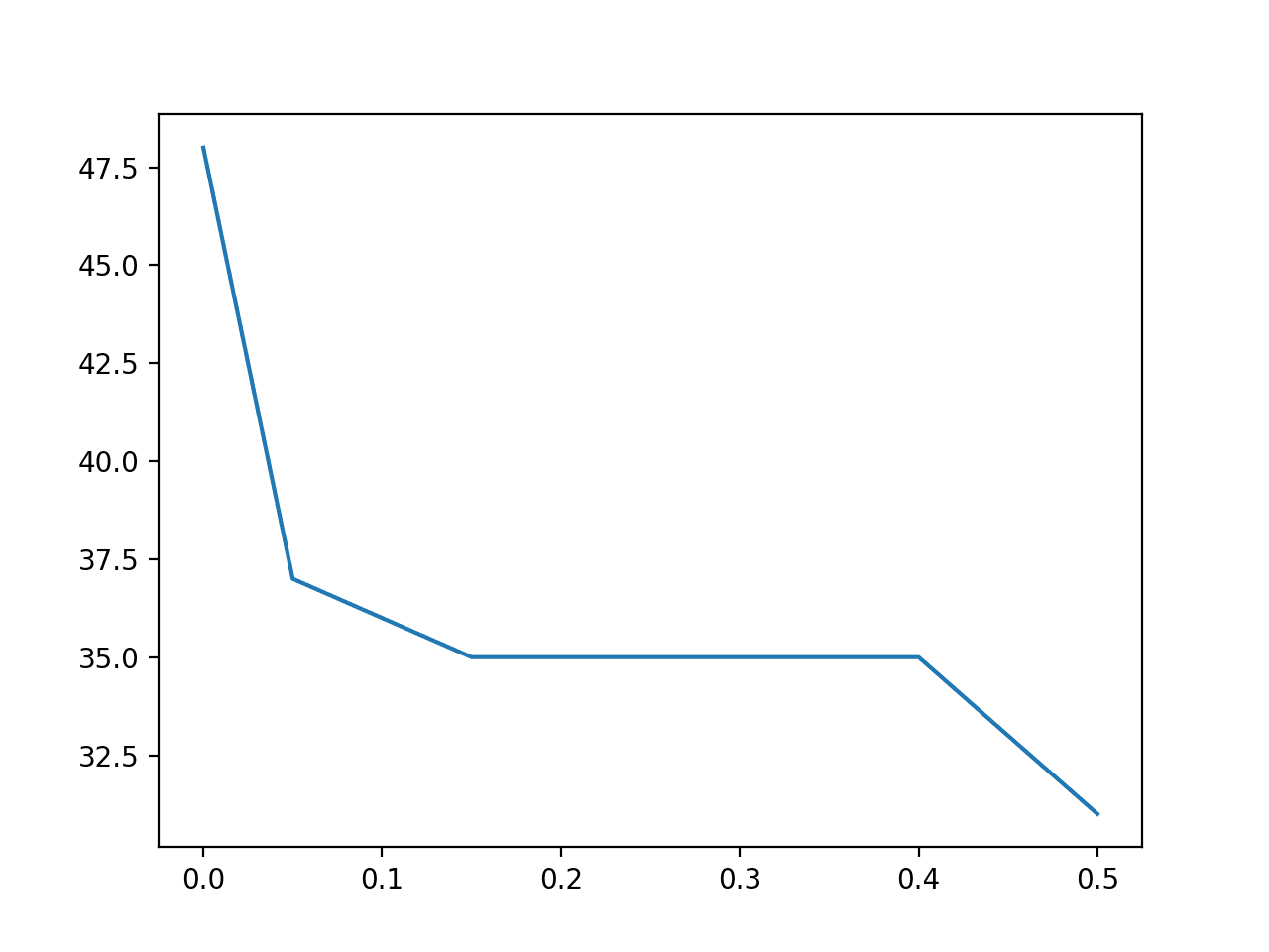
Line Plot of Variance Threshold (X) Versus Number of Selected Features (Y)
Identify Rows That Contain Duplicate Data
Rows that have identical data are probably useless, if not dangerously misleading during model evaluation.
Here, a duplicate row is a row where each value in each column for that row appears in identically the same order (same column values) in another row.
… if you have used raw data that may have duplicate entries, removing duplicate data will be an important step in ensuring your data can be accurately used.
— Page 173, Data Wrangling with Python, 2016.
From a probabilistic perspective, you can think of duplicate data as adjusting the priors for a class label or data distribution. This may help an algorithm like Naive Bayes if you wish to purposefully bias the priors. Typically, this is not the case and machine learning algorithms will perform better by identifying and removing rows with duplicate data.
From an algorithm evaluation perspective, duplicate rows will result in misleading performance. For example, if you are using a train/test split or k-fold cross-validation, then it is possible for a duplicate row or rows to appear in both train and test datasets and any evaluation of the model on these rows will be (or should be) correct. This will result in an optimistically biased estimate of performance on unseen data.
Data deduplication, also known as duplicate detection, record linkage, record matching, or entity resolution, refers to the process of identifying tuples in one or more relations that refer to the same real-world entity.
— Page 47, Data Cleaning, 2019.
If you think this is not the case for your dataset or chosen model, design a controlled experiment to test it. This could be achieved by evaluating model skill with the raw dataset and the dataset with duplicates removed and comparing performance. Another experiment might involve augmenting the dataset with different numbers of randomly selected duplicate examples.
The pandas function duplicated() will report whether a given row is duplicated or not. All rows are marked as either False to indicate that it is not a duplicate or True to indicate that it is a duplicate. If there are duplicates, the first occurrence of the row is marked False (by default), as we might expect.
The example below checks for duplicates.
|
1 2 3 4 5 6 7 8 9 10 11 12 |
# locate rows of duplicate data from pandas import read_csv # define the location of the dataset path = 'https://raw.githubusercontent.com/jbrownlee/Datasets/master/iris.csv' # load the dataset df = read_csv(path, header=None) # calculate duplicates dups = df.duplicated() # report if there are any duplicates print(dups.any()) # list all duplicate rows print(df[dups]) |
Running the example first loads the dataset, then calculates row duplicates.
First, the presence of any duplicate rows is reported, and in this case, we can see that there are duplicates (True).
Then all duplicate rows are reported. In this case, we can see that three duplicate rows that were identified are printed.
|
1 2 3 4 5 |
True 0 1 2 3 4 34 4.9 3.1 1.5 0.1 Iris-setosa 37 4.9 3.1 1.5 0.1 Iris-setosa 142 5.8 2.7 5.1 1.9 Iris-virginica |
Delete Rows That Contain Duplicate Data
Rows of duplicate data should probably be deleted from your dataset prior to modeling.
If your dataset simply has duplicate rows, there is no need to worry about preserving the data; it is already a part of the finished dataset and you can merely remove or drop these rows from your cleaned data.
— Page 186, Data Wrangling with Python, 2016.
There are many ways to achieve this, although Pandas provides the drop_duplicates() function that achieves exactly this.
The example below demonstrates deleting duplicate rows from a dataset.
|
1 2 3 4 5 6 7 8 9 10 |
# delete rows of duplicate data from the dataset from pandas import read_csv # define the location of the dataset path = 'https://raw.githubusercontent.com/jbrownlee/Datasets/master/iris.csv' # load the dataset df = read_csv(path, header=None) print(df.shape) # delete duplicate rows df.drop_duplicates(inplace=True) print(df.shape) |
Running the example first loads the dataset and reports the number of rows and columns.
Next, the rows of duplicated data are identified and removed from the DataFrame. Then the shape of the DataFrame is reported to confirm the change.
|
1 2 |
(150, 5) (147, 5) |
Further Reading
This section provides more resources on the topic if you are looking to go deeper.
Tutorials
Books
- Data Cleaning, 2019.
- Data Wrangling with Python, 2016.
- Feature Engineering and Selection, 2019.
APIs
- numpy.unique API.
- pandas.DataFrame.nunique API.
- sklearn.feature_selection.VarianceThreshold API.
- pandas.DataFrame.drop API.
- pandas.DataFrame.duplicated API.
- pandas.DataFrame.drop_duplicates API.
Summary
In this tutorial, you discovered basic data cleaning you should always perform on your dataset.
Specifically, you learned:
- How to identify and remove column variables that only have a single value.
- How to identify and consider column variables with very few unique values.
- How to identify and remove rows that contain duplicate observations.
Do you have any questions?
Ask your questions in the comments below and I will do my best to answer.
Get a Handle on Modern Data Preparation!

Prepare Your Machine Learning Data in Minutes
...with just a few lines of python code
Discover how in my new Ebook:
Data Preparation for Machine Learning
It provides self-study tutorials with full working code on:
Feature Selection, RFE, Data Cleaning, Data Transforms, Scaling, Dimensionality Reduction,
and much more...


nice work
Thanks.
Hi Jason,
May I know the reasons why delete columns that have unique values?
Please enlighten me. Thanks.
We delete columns that do not have many unique values because they do not or are likely to not contribute to the target variable.
Thanks. I am using R and I am considering to learn Python. Do you know if there is a tutorial about this same topic (how to clean datasets) for R?
Is it worth to combine Python and R?
I don’t know off hand, sorry.
I recommend sticking to one platform.
I really enjoyed the Tutorial.
Thanks!
Great article sometimes we forget the basics when building ML. Thanks Jason
Thanks!
Yes, we sure do.
Thanks for the tutorial. It’s giving us more options for cleaning.
Thanks.
Good thinking in the tutorial. I like the approach of identification of non – unique data. I work in industrial computing and we tend to have a lot of constant “1 / 0 ” entries for when valves are open and shut, but for a time period, removing a constant value would help identify errors.
Thanks for the thoughts!
Thanks.
Nice tutorial, thanks. You have a few articles about clean, evaluate features,.. Do you have a book with everything?
Not at this stage, hopefully in the future.
Does a process of removing/filling Nan instances belong to data cleaning as well? I guess it shall be performed even before the steps covered by your article.
Regards!
Yes!
Nice tutorial thank you. I am new here and want to ask that do you have any tutorial for the training of ML model by aggregating the data for more than one location?
You’re welcome.
Perhaps this will give you ideas:
https://machinelearningmastery.com/faq/single-faq/how-to-develop-forecast-models-for-multiple-sites
Hi,
I’m working with an image Dataset (my model takes as input two images (an image and its ground truth)). I want to do a data Cleaning for my database. There is no tutorial about how to proceed (all tutorials work with a CSV dataset). Can you please guide me on how to do so. Think you very much for your time.
Yes, you can see tutorials on working with images here:
https://machinelearningmastery.com/start-here/#dlfcv
Dear Dr Jason,
Thank you for the article.
I need clarification on the how unique and nunique operate. Do these functions operate row-wise or column-wise.
Steps needed to replicate.
I need clarification on the counts. Given that there are 50 features and 937 rows, from the above code, for example what does, 238, 297, 927, 933, 179 mean.
Does that mean there are 238 counts, or 238 is the unique number?
Or does that mean the unique number in each of the 50 columns are 238, 297, 927,933, 179.
Or does that mean for example that in the first column there are 238 unique values?
Reference
Example 1, at https://numpy.org/doc/stable/reference/generated/numpy.unique.html
Thank you,
Anthony of Sydney
Dear Dr Jason,
I used a smaller dataset and understood it now. Summary appears after background program.
I understand this. I will ask you after the summary of the count/tally of each unique number.
Summary:
unique and DataFrame’s nunique work in the same way.
Each column produces a count of the unique occurrence of a number by invocation of unique() and df.nunique().
If unique and df.unique were invoked without the () then we print out the whole matrix.
Question:
How do we tally and/or have a frequency of each number in the column.
Thank you,
Anthony of Sydney
Dear Dr Jason,
A slight correction.
unique(stuff) – produces a list of the numbers. It does not produce a count.
To find out a unique number of numbers from using the unique operator.
Excuse my pun, but it is not the unique way of determining the number of unique numbers in each column.
My question remains:
How do we tally and/or have a frequency of each number in the column?
Thank you,
Anthony of Sydney
You must specify the axis along which to count unique values, perhaps check the documentation for the function.
Unique values are column wise.
Dear Dr Jason,
I wasn’t clear again.
Before I proceed with what I intended is that:
* numpy’s unique and DataFrame’s nunique operate column-wise as I have discovered above.
My original question was about counting tallies for each feature=column.
What I want to share is the tally/frequency of unique numbers in a matrix.
It uses the numpy’s unique function BUT with the parameter numpy.unique(stuff,return_counts = True)
Here is the code to find a tally of frequency/count of unique numbers in the overall matrix
Now let’s get a frequency/tally of unique numbers for each feature = column
Maybe the presentation of the counts/frequencies tally for each feature=column could be tidied up.
The method above for the whole of matrix or for each column=feature is not unique. The implementation was inspired by code at https://kite.com/python/answers/how-to-count-frequency-of-unique-values-in-a-numpy-array-in-python
You can get a similar result with counts/frequencies tally for each feature=column
Source for inspiration: section titled Class collections.Counter at https://docs.python.org/2/library/collections.html
Conclusions:
This is NOT about the unique/nunique techniques for determining the counts of features.
Rather I have presented two techniques for finding the counts/tallies of each column using the unique with parameter return_counts=True while the other uses the collections’ Counter.
Thank you,
Anthony of Sydney
Thanks for sharing.
Thanks for the article, Jason! I really enjoyed the Tutorial.
You’re welcome, I’m happy to hear that.
Dear Dr. Brownlee,
Thank you for nice article. I have a doubt that can we use VarianceThreshold() to remove object data types as well? If not, are there alternative methods of doing it?
Or do you recommend this step to do after data transform?
Thanks,
Swati
You’re welcome.
What do you mean object types? E.g. strings? categories?
Yes, I believe it will work for those data types – at least in principle. Try it and see.
Hi Jason, Great article!
I just have one doubt regarding the threshold. If we are taking threshold as 0.5, does that mean we are saying if the variable is having 95% same values or higher remove that variable?
Similarly, for 0.8 threshold, if the variable is having 92% or higher same values remove te variable?
If removing a variable results in better model performance, then I recommend that you remove it.
I think you misunderstood my question.
I was talking about the threshold. What does threshold 0.5 means
You can learn about thresholds for predicted probabilities here:
https://machinelearningmastery.com/threshold-moving-for-imbalanced-classification/
# example of apply the variance threshold
from pandas import read_csv
from sklearn.feature_selection import VarianceThreshold
# define the location of the dataset
path = ‘https://raw.githubusercontent.com/jbrownlee/Datasets/master/oil-spill.csv’
# load the dataset
df = read_csv(path, header=None)
# split data into inputs and outputs
data = df.values
X = data[:, :-1]
y = data[:, -1]
print(X.shape, y.shape)
# define the transform
transform = VarianceThreshold()
# transform the input data
X_sel = transform.fit_transform(X)
print(X_sel.shape)
In this example you are using X = data[:, :-1] which do not include the last column. why we are not including last column.
X is the input data, we do not include the output variable as part of the input.
Hi Jason,
As always, thank you for your amazing tutorials.
I have a question. My dataset is highly imbalanced and there lies some ambiguity (same input but different class label). Do you think its better to “re-assign” ambiguous data points from the majority class label to the minority class label? (since I care more about the minority class) Or its just better to filter those data points out?
P.S: I am considering class weights while training.
You’re welcome.
Excellent question! Try a few strategies for dealing with the ambiguous data and see what works best, e.g. try removing, try re-labelling, etc.
Hi Jason,
Thank you for the tutorial. Very informative!
I have a question regarding features with a constant value. For a classification problem, I have a feature vector of length 80 where 4 of the features are always zero. I get almost the same result using different classifiers (SVM, random forest, logistic regression and two different deep learning models) with and without removing the zero features. Is it because the percentage of the zero feature to the total number of features is small (4/80)?
Following this question, apart from computation efficiency, if the portion of features with constant value or very small variance is quite small compared to the total number of features, do we end up with almost the same classification scores whether we keep or remove these features with a constant value or a very small variance? In such cases, are there classifiers for which removing or keeping such features could make a difference in classification scores?
Thank you for your help!
You’re welcome.
If a variable always has the same value, it must be removed from the dataset.
Perhaps you can try alternate data preparation, alternate models, alternate model configurations, alternate metrics, etc.
Thank you for your response.
In general, if you remove variable(s) with constant zero value for all the observations, do you expect to see any degradation in the classification scores (like accuracy and F-score)?
Removing low variance data will improve the efficiency of the method and sometimes the performance.
Is there any chance of degradation in the performance of the model? And if, like in my case, there is almost no change or quite minimal change (like in the order of 10th of a percent) in the classification scores, is there any reason behind that?
I was thinking for a neural network, the weights of those features with zero value won’t play a role as their multiplication with the feature is always zero (I understand when the number of features with zero value or constant variance increases it can create numerical issues). So, does it actually make any difference for a neural network when the number of features with zero value is small?
Perhaps. Evaluate with and without and discover the answer for your data and model.
Sorry for asking you so many questions.
Can you think of any reason why performance of a model might degrade despite removing features that do not convey any information (like features that are always zero or have a constant variance in general)?
Yes, the assumption that the features are not relevant could be false.
I just wanted to make a clarification about my question. Where I said: “I get almost the same result using different classifiers (SVM, random forest, logistic regression and two different deep learning models) with and without removing the zero features.”, I meant getting almost the same result for each classifier whether I keep those zero features or not. I didn’t mean I got the same result for all the classifiers.
Hi Jason,
very nice tutorial!. Thank you.
I see pandas dataframe as a very powerful tools to clean, replace and filter tabular dataset on .csv and excel files, e.g.. There are many pandas methods I did not know !.
Anyway, I was a little confused about the fact that you can get, for example, all the columns that have a zero value, or any other weird values such as strings etc. constructing a command like the following:
n_0 = (dataframe == 0).sum()
But, if you apply the same “structure” to get all the columns ‘NaN’ values, such as :
n_nan= (datataframe ==np.nan).sum()
It does not work!!
instead, you have to go through this one:
n_nan = dataframe.isnull.sum()
certain logic pandas path fail! 🙁
regards,
You’re welcome.
Yes, nan is special. Equality does not work I believe.
Hi sir, great explanation. How to decide and find the best threshold used in variance threshold for filtering possible useless features for modelling if my data has been normalized with z-score normalization? I’m trying to do feature reduction to find best subset of features to build my calibrated sigmoid SVC model on cross-validated training data. I’ve been using threshold 0, 0.01, 0.003, and (.8 * (1 – .8)) but no feautures are filtered.
This tutorial may help:
https://machinelearningmastery.com/threshold-moving-for-imbalanced-classification/
I cam see how removal of columns of a single variable apply to traditional ML. Does it apply neural network type ML as well?
Yes, feature selection can help neural nets.
Hi sir, great article. I have tried the methods you proposed and could see them work well already but I’m just curious if performing PCA on my dataset before feeding it to a neural net would do any better? Or would the hidden layers figure the principal components automatically while learning weights?
Perhaps try it and see.
Receiving error messages: not found in axis.
# record columns to delete
to_del = [i for i,v in enumerate(counts) if (float(v)/df.shape[0]*100) < 1]
print(to_del)
????
Worked out well by printing out the value
# drop useless columns
df.drop(to_del, axis=1, inplace=True)
????
But this one is generating error message: not found in axis.
Please how can I resolved this?
Sorry to hear that you’re having trouble, these tips may help:
https://machinelearningmastery.com/faq/single-faq/why-does-the-code-in-the-tutorial-not-work-for-me
Hi, I have 1472 news headlines dataset comprising 1172 with label ‘positive’ and ‘302’ negative. Is this dataset could be called as unbalanced?
and these 1472 news headlines have 170 duplicate records. With 29 negative and 141 positive. when i remove duplicates and implement my approach 1 with bert model and svm i got more accuracy .but when i remove duplicates and implement my approach 2 with corenlp dependencies uni gram ,bigram and tfidf with svm i got less accuracy . my question is Why there is a difference of removing duplicates on two approaches .
I am not exactly sure. This is possibly one of the reason: https://machinelearningmastery.com/different-results-each-time-in-machine-learning/
Hi Adrian, your tutorials are awesome. I learned a lot from your most of the blogs.
I have one question regarding the data cleaning method. I am looking for creating an algorithm that can detect errors in the data (duplicate, missing, incorrect, inconsistency, outlier, noisy data, etc…) and replace them with suitable values while reducing the errors in the dataset.
Do you have any source or paper that can help me to develop the algorithm that can perform this task?
Your help will be appreciated.
Hi Anonymous…you are describing a concept called “data imputation”. The following may help clarify.
https://machinelearningmastery.com/handle-missing-data-python/
Hi Jason,
For column with multiple unique values,
For eg: Email Column,
I am extracting the domain names and bucketizing to different categories,
Is this the good way of handling string column with too many values.
and
To do bucketing, we need to see the different values in first place, am I right?
for in case if there is typos in domain names, we have to sanitize that. eg: yahoo, yahooo, yhaoo -> bucket as “yahoo”
Hi Justin…Bucketing may be a reasonable approach. Have you implemented this preprocessing step yet?
Thanks for the reply, I am cleaning the data, the data is 15 million, I should extract the unique values, clean them, then only I should start the bucketing, Am I Correct?
Hi Jason,
In the post there is a part to remove columns that have low variance. Then it shows 14 features can be removed. How can we know which columns that can be removed?
Thanks