Supervised learning in machine learning can be described in terms of function approximation.
Given a dataset comprised of inputs and outputs, we assume that there is an unknown underlying function that is consistent in mapping inputs to outputs in the target domain and resulted in the dataset. We then use supervised learning algorithms to approximate this function.
Neural networks are an example of a supervised machine learning algorithm that is perhaps best understood in the context of function approximation. This can be demonstrated with examples of neural networks approximating simple one-dimensional functions that aid in developing the intuition for what is being learned by the model.
In this tutorial, you will discover the intuition behind neural networks as function approximation algorithms.
After completing this tutorial, you will know:
- Training a neural network on data approximates the unknown underlying mapping function from inputs to outputs.
- One dimensional input and output datasets provide a useful basis for developing the intuitions for function approximation.
- How to develop and evaluate a small neural network for function approximation.
Kick-start your project with my new book Deep Learning With Python, including step-by-step tutorials and the Python source code files for all examples.
Let’s get started.
Neural Networks are Function Approximation Algorithms
Photo by daveynin, some rights reserved.
Tutorial Overview
This tutorial is divided into three parts; they are:
- What Is Function Approximation
- Definition of a Simple Function
- Approximating a Simple Function
What Is Function Approximation
Function approximation is a technique for estimating an unknown underlying function using historical or available observations from the domain.
Artificial neural networks learn to approximate a function.
In supervised learning, a dataset is comprised of inputs and outputs, and the supervised learning algorithm learns how to best map examples of inputs to examples of outputs.
We can think of this mapping as being governed by a mathematical function, called the mapping function, and it is this function that a supervised learning algorithm seeks to best approximate.
Neural networks are an example of a supervised learning algorithm and seek to approximate the function represented by your data. This is achieved by calculating the error between the predicted outputs and the expected outputs and minimizing this error during the training process.
It is best to think of feedforward networks as function approximation machines that are designed to achieve statistical generalization, occasionally drawing some insights from what we know about the brain, rather than as models of brain function.
— Page 169, Deep Learning, 2016.
We say “approximate” because although we suspect such a mapping function exists, we don’t know anything about it.
The true function that maps inputs to outputs is unknown and is often referred to as the target function. It is the target of the learning process, the function we are trying to approximate using only the data that is available. If we knew the target function, we would not need to approximate it, i.e. we would not need a supervised machine learning algorithm. Therefore, function approximation is only a useful tool when the underlying target mapping function is unknown.
All we have are observations from the domain that contain examples of inputs and outputs. This implies things about the size and quality of the data; for example:
- The more examples we have, the more we might be able to figure out about the mapping function.
- The less noise we have in observations, the more crisp approximation we can make of the mapping function.
So why do we like using neural networks for function approximation?
The reason is that they are a universal approximator. In theory, they can be used to approximate any function.
… the universal approximation theorem states that a feedforward network with a linear output layer and at least one hidden layer with any “squashing” activation function (such as the logistic sigmoid activation function) can approximate any […] function from one finite-dimensional space to another with any desired non-zero amount of error, provided that the network is given enough hidden units
— Page 198, Deep Learning, 2016.
Regression predictive modeling involves predicting a numerical quantity given inputs. Classification predictive modeling involves predicting a class label given inputs.
Both of these predictive modeling problems can be seen as examples of function approximation.
To make this concrete, we can review a worked example.
In the next section, let’s define a simple function that we can later approximate.
Definition of a Simple Function
We can define a simple function with one numerical input variable and one numerical output variable and use this as the basis for understanding neural networks for function approximation.
We can define a domain of numbers as our input, such as floating-point values from -50 to 50.
We can then select a mathematical operation to apply to the inputs to get the output values. The selected mathematical operation will be the mapping function, and because we are choosing it, we will know what it is. In practice, this is not the case and is the reason why we would use a supervised learning algorithm like a neural network to learn or discover the mapping function.
In this case, we will use the square of the input as the mapping function, defined as:
- y = x^2
Where y is the output variable and x is the input variable.
We can develop an intuition for this mapping function by enumerating the values in the range of our input variable and calculating the output value for each input and plotting the result.
The example below implements this in Python.
|
1 2 3 4 5 6 7 8 9 10 11 12 |
# example of creating a univariate dataset with a given mapping function from matplotlib import pyplot # define the input data x = [i for i in range(-50,51)] # define the output data y = [i**2.0 for i in x] # plot the input versus the output pyplot.scatter(x,y) pyplot.title('Input (x) versus Output (y)') pyplot.xlabel('Input Variable (x)') pyplot.ylabel('Output Variable (y)') pyplot.show() |
Running the example first creates a list of integer values across the entire input domain.
The output values are then calculated using the mapping function, then a plot is created with the input values on the x-axis and the output values on the y-axis.
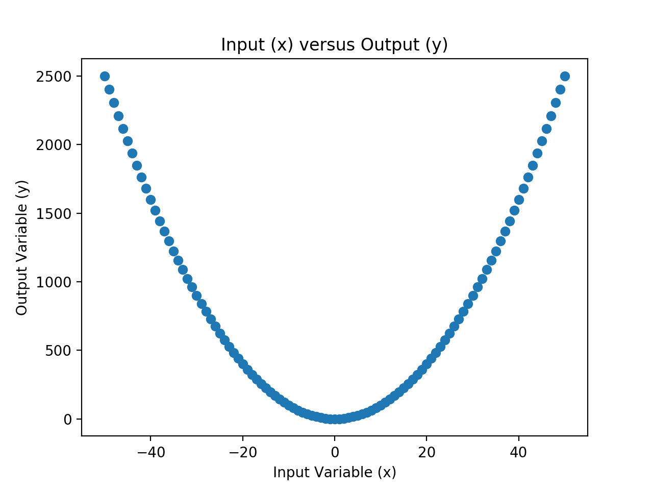
Scatter Plot of Input and Output Values for the Chosen Mapping Function
The input and output variables represent our dataset.
Next, we can then pretend to forget that we know what the mapping function is and use a neural network to re-learn or re-discover the mapping function.
Approximating a Simple Function
We can fit a neural network model on examples of inputs and outputs and see if the model can learn the mapping function.
This is a very simple mapping function, so we would expect a small neural network could learn it quickly.
We will define the network using the Keras deep learning library and use some data preparation tools from the scikit-learn library.
First, let’s define the dataset.
|
1 2 3 4 5 |
... # define the dataset x = asarray([i for i in range(-50,51)]) y = asarray([i**2.0 for i in x]) print(x.min(), x.max(), y.min(), y.max()) |
Next, we can reshape the data so that the input and output variables are columns with one observation per row, as is expected when using supervised learning models.
|
1 2 3 4 |
... # reshape arrays into into rows and cols x = x.reshape((len(x), 1)) y = y.reshape((len(y), 1)) |
Next, we will need to scale the inputs and the outputs.
The inputs will have a range between -50 and 50, whereas the outputs will have a range between -50^2 (2500) and 0^2 (0). Large input and output values can make training neural networks unstable, therefore, it is a good idea to scale data first.
We can use the MinMaxScaler to separately normalize the input values and the output values to values in the range between 0 and 1.
|
1 2 3 4 5 6 7 |
... # separately scale the input and output variables scale_x = MinMaxScaler() x = scale_x.fit_transform(x) scale_y = MinMaxScaler() y = scale_y.fit_transform(y) print(x.min(), x.max(), y.min(), y.max()) |
We can now define a neural network model.
With some trial and error, I chose a model with two hidden layers and 10 nodes in each layer. Perhaps experiment with other configurations to see if you can do better.
|
1 2 3 4 5 6 |
... # design the neural network model model = Sequential() model.add(Dense(10, input_dim=1, activation='relu', kernel_initializer='he_uniform')) model.add(Dense(10, activation='relu', kernel_initializer='he_uniform')) model.add(Dense(1)) |
We will fit the model using a mean squared loss and use the efficient adam version of stochastic gradient descent to optimize the model.
This means the model will seek to minimize the mean squared error between the predictions made and the expected output values (y) while it tries to approximate the mapping function.
|
1 2 3 |
... # define the loss function and optimization algorithm model.compile(loss='mse', optimizer='adam') |
We don’t have a lot of data (e.g. about 100 rows), so we will fit the model for 500 epochs and use a small batch size of 10.
Again, these values were found after a little trial and error; try different values and see if you can do better.
|
1 2 3 |
... # ft the model on the training dataset model.fit(x, y, epochs=500, batch_size=10, verbose=0) |
Once fit, we can evaluate the model.
We will make a prediction for each example in the dataset and calculate the error. A perfect approximation would be 0.0. This is not possible in general because of noise in the observations, incomplete data, and complexity of the unknown underlying mapping function.
In this case, it is possible because we have all observations, there is no noise in the data, and the underlying function is not complex.
First, we can make the prediction.
|
1 2 3 |
... # make predictions for the input data yhat = model.predict(x) |
We then must invert the scaling that we performed.
This is so the error is reported in the original units of the target variable.
|
1 2 3 4 5 |
... # inverse transforms x_plot = scale_x.inverse_transform(x) y_plot = scale_y.inverse_transform(y) yhat_plot = scale_y.inverse_transform(yhat) |
We can then calculate and report the prediction error in the original units of the target variable.
|
1 2 3 |
... # report model error print('MSE: %.3f' % mean_squared_error(y_plot, yhat_plot)) |
Finally, we can create a scatter plot of the real mapping of inputs to outputs and compare it to the mapping of inputs to the predicted outputs and see what the approximation of the mapping function looks like spatially.
This is helpful for developing the intuition behind what neural networks are learning.
|
1 2 3 4 5 6 7 8 |
... # plot x vs yhat pyplot.scatter(x_plot,yhat_plot, label='Predicted') pyplot.title('Input (x) versus Output (y)') pyplot.xlabel('Input Variable (x)') pyplot.ylabel('Output Variable (y)') pyplot.legend() pyplot.show() |
Tying this together, the complete example is listed below.
|
1 2 3 4 5 6 7 8 9 10 11 12 13 14 15 16 17 18 19 20 21 22 23 24 25 26 27 28 29 30 31 32 33 34 35 36 37 38 39 40 41 42 43 44 45 46 |
# example of fitting a neural net on x vs x^2 from sklearn.preprocessing import MinMaxScaler from sklearn.metrics import mean_squared_error from keras.models import Sequential from keras.layers import Dense from numpy import asarray from matplotlib import pyplot # define the dataset x = asarray([i for i in range(-50,51)]) y = asarray([i**2.0 for i in x]) print(x.min(), x.max(), y.min(), y.max()) # reshape arrays into into rows and cols x = x.reshape((len(x), 1)) y = y.reshape((len(y), 1)) # separately scale the input and output variables scale_x = MinMaxScaler() x = scale_x.fit_transform(x) scale_y = MinMaxScaler() y = scale_y.fit_transform(y) print(x.min(), x.max(), y.min(), y.max()) # design the neural network model model = Sequential() model.add(Dense(10, input_dim=1, activation='relu', kernel_initializer='he_uniform')) model.add(Dense(10, activation='relu', kernel_initializer='he_uniform')) model.add(Dense(1)) # define the loss function and optimization algorithm model.compile(loss='mse', optimizer='adam') # ft the model on the training dataset model.fit(x, y, epochs=500, batch_size=10, verbose=0) # make predictions for the input data yhat = model.predict(x) # inverse transforms x_plot = scale_x.inverse_transform(x) y_plot = scale_y.inverse_transform(y) yhat_plot = scale_y.inverse_transform(yhat) # report model error print('MSE: %.3f' % mean_squared_error(y_plot, yhat_plot)) # plot x vs y pyplot.scatter(x_plot,y_plot, label='Actual') # plot x vs yhat pyplot.scatter(x_plot,yhat_plot, label='Predicted') pyplot.title('Input (x) versus Output (y)') pyplot.xlabel('Input Variable (x)') pyplot.ylabel('Output Variable (y)') pyplot.legend() pyplot.show() |
Running the example first reports the range of values for the input and output variables, then the range of the same variables after scaling. This confirms that the scaling operation was performed as we expected.
The model is then fit and evaluated on the dataset.
Note: Your results may vary given the stochastic nature of the algorithm or evaluation procedure, or differences in numerical precision. Consider running the example a few times and compare the average outcome.
In this case, we can see that the mean squared error is about 1,300, in squared units. If we calculate the square root, this gives us the root mean squared error (RMSE) in the original units. We can see that the average error is about 36 units, which is fine, but not great.
What results did you get? Can you do better?
Let me know in the comments below.
|
1 2 3 |
-50 50 0.0 2500.0 0.0 1.0 0.0 1.0 MSE: 1300.776 |
A scatter plot is then created comparing the inputs versus the real outputs, and the inputs versus the predicted outputs.
The difference between these two data series is the error in the approximation of the mapping function. We can see that the approximation is reasonable; it captures the general shape. We can see that there are errors, especially around the 0 input values.
This suggests that there is plenty of room for improvement, such as using a different activation function or different network architecture to better approximate the mapping function.
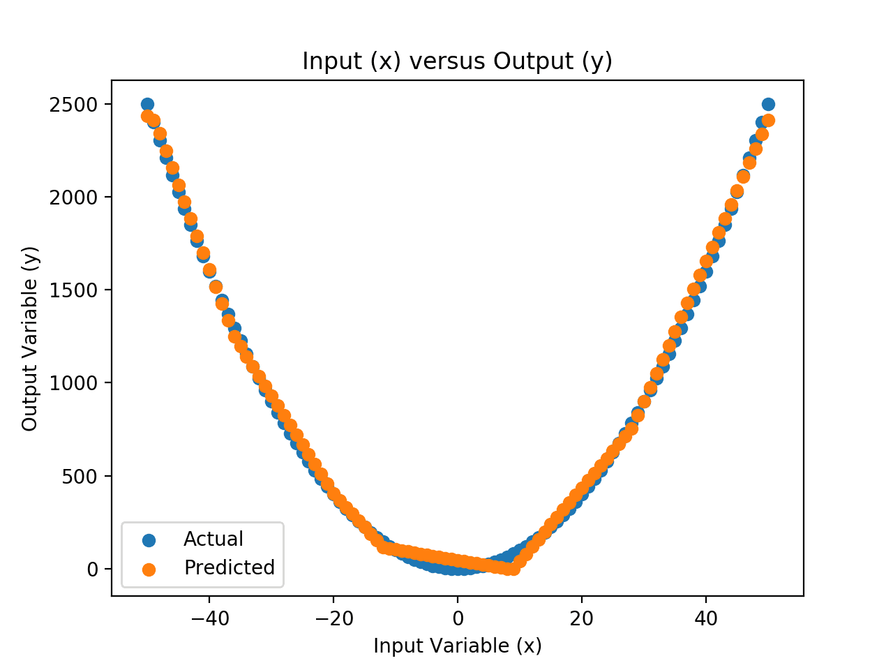
Scatter Plot of Input vs. Actual and Predicted Values for the Neural Net Approximation
Further Reading
This section provides more resources on the topic if you are looking to go deeper.
Tutorials
Books
- Deep Learning, 2016.
Articles
Summary
In this tutorial, you discovered the intuition behind neural networks as function approximation algorithms.
Specifically, you learned:
- Training a neural network on data approximates the unknown underlying mapping function from inputs to outputs.
- One dimensional input and output datasets provide a useful basis for developing the intuitions for function approximation.
- How to develop and evaluate a small neural network for function approximation.
Do you have any questions?
Ask your questions in the comments below and I will do my best to answer.

")


May I suggest to generate random values as x_hat and predict y_hat. That would be more realistic. You may even want to get random values for x and calculate y.
Great suggestion, thanks.
I also suggest scatter of residuals (y-y_hat) in the y-axis and your input variable in the x-axis to check for discernible patterns. A discernible pattern implies the function approximation needs improvement.
Great suggestion! Always look at your residuals.
Function approximation is exactly what nonparametric regressions do. For an introduction to them see here ( https://cran.r-project.org/web/packages/NNS/vignettes/NNSvignette_Clustering_and_Regression.html ) and for an extension to their use in machine learning, both continuous and discrete classification problems see here ( https://github.com/OVVO-Financial/NNS/tree/NNS-Beta-Version/examples#3-machine-learning)
To the problem at hand, using the above referenced NNS techniques, the MSE can do exceptionally better than the NN demonstrated.
In R:
> library(NNS)
> x = seq(-50,50,1); y = x^2
> y.hat = NNS.reg(x,y)$Fitted.xy$y.hat
> mean((y.hat – y)^2)
[1] 149.4403
Nice, thanks for sharing!
YW! This article does a good job explaining the importance of function approximation and its extensions.
Thanks.
There is however the dilution problem with conventional artificial neural networks when there is only one non-linear term per n weights. Where n is the width of the network. That means with say a ReLU network there are fewer ‘break-points’ than if you had 1 non-linear term (ReLU output) per weight. Giving poor fitting.
I would say (not giving myself airs) neural network researchers should go back and look at the basics of what they are doing.
https://ai462qqq.blogspot.com/2019/11/artificial-neural-networks.html
https://discourse.numenta.org/t/and-there-they-stopped/7293
Thanks for sharing.
Love this succinct summary of what i consider to be one of the most overlooked and yet fundamental concepts in ML (that you are approximating a function). Given your abilities I would love to see you do your take on no free lunch. Any chance you would do an article on a clear explanation of no free lunch? 🙂
Thanks.
Great suggestion, I know it well. The take away is the reminder that you should use careful and extensive experiments rather than favourite algorithm to get the best results for a problem.
I think it could also be helpful as others have mentioned to augment the article with a couple small additions (or maybe include in a followup). You could next add a small normal curve error around the observed y values and show what happens and explain why this is important to know about. Another thing you could do something like chopping off a bit of the two sides (the lowest and highest x values) and then show the effect of overfitting by showing how the NN handles the edges once it runs out of training examples. The expectation here for me would be that if you dont train properly for overfitting once the NN hits the edges it may not know what to do. If trained correctly w test and train sets etc it then may continue well along the edges and keep following the y=x^2 curve.
Great extension!
Well organized and very good presentation. I love to read your articles.
An other suggestion is an article about function approximation and multi-value data. Functions such as x^2 , sinx, cosx, …..is one of them. It will be very interesting,
Thanks.
Great suggestion.
Hi Jason! I love your tutorials. I was just reviewing this same topic using essentially the same problem via a Tensorflow introduction (https://colab.research.google.com/github/lmoroney/mlday-tokyo/blob/master/Lab1-Hello-ML-World.ipynb), and I was struck with the piecewise-linear nature of the approximation, and the fact that it was an asymmetric fit to a symmetric function. I tried different numbers of hidden neurons, different activations, and different number of epochs to try to better understand the shape of the approximation as a function of these variables. Do you have any general comments to add on these matters? Such reflections could be a useful addition to this tutorial, which otherwise seems to end abruptly.
Try changing the activation function in the hidden layer to sigmoid.
Ok…but I’d already done that before asking the question.
Thanks.
The “why” is hard for neural nets.
For a given model, we could explore the calculation of each node and understand how specific outputs came to be. Very time consuming with not a lot of payoff if we are focused on model skill for a predictive modeling problem. I generally try to stay away from crafting a “why” narrative for models:
https://machinelearningmastery.com/faq/single-faq/how-do-i-interpret-the-predictions-from-my-model
Hi Jason,
Great Function Approx. Tutorial. I like it!
Before working on your different tutorial using GAN, for function approach ( I am excited about this radical “Adversarial Nets approach”!), I decided to spend some time on this one.
Here, I share my “experiments” based on variations on your script. Thanks you for offering such as simple and tested code.
My comments:
1º) In y opinion Functions or data fitting approach are related mathematically to Taylor series, Least Squares methods (solved on python with library “scipy.optimize.curve_fit( )”), etc. But in this case of NN we do not have to have a previous assumption about the kind of f(x) … we just fitted the data !!. So it is a more advance method, in my opinion…
2º) I added others layers to the 3 dense layers, such as BatchNormalization(), Dropout,() I also used l1_l2 regularizers, but I get even worse results that your basic and simple model of 3 dense layers!
3º) I change the numbers of 10 units in dense layer to higher (50,100,…) and lower (5, ) , But I did not get any improvement about your optimum one.
4º) I decided not to use normalized data (such as MinMaxScaler()) so I tested raw (X,Y) data…without normalization …and surprisingly the code continuing performing well , on a stable way…My only observation it is demanded more (X,Y) samples !
5º) I also tested Cubic functions (X^3), besides quadratics and linear…for all of them they fit pretty well the whole data bunch … But with more samples and more epochs I got lower ‘root mean squared error’ up to a limit around 0.03
6º) I decided to test also trigonometric functions (sine) with the same architecture and model and it is was ver good performed.
7º) I decided to test exponential functions (a+e^bx+c) with the same architecture and model and it also was very good performed.
So your model it is very simple and robust and performs very well for all that cases …My only “finding”, after all these experiments it is that outside of the dataset learning range (Xmin-Xmax, Ymin-Ymax), when I tested values out range …the approach or NN model prediction start to get worse …the more outside …the more bads…So it learns well the data inside range …but it can not generalizes well outside that range …unless you know the kind of functions to apply subsequent methods such as “scipy.optimize.curve-fit()”…but in this case you need to assume the type of expected function and predicted behaviour on values outside range.
This is the reason because I prefer the “honesty” of NN …because outside of range values … you can affirm nothing !…There is not values to test it!
As I said before I am excited about how can GAN approach handle these learnings on functions approaching vs this very simple NN approach!
regards,
JG
Very cool, well done!
Depending on the form of the function, the neural nets may or may not extrapolate well. In this case not so well. Functions might be a little too nonlinear and the model a little too simple.
It might be fun to limit training to subsets of the valid input space and see if it can learn to interpolate correctly. I expect it can. This would show it at least learns a viable approximation within the domain – related to your extrapolation experiments.
You could write your experiments up as a tutorial, I’d post them in a heart beat!
Hi Jason,
More COMMENTS on my experiments!.
I review several of the NN function approaches experiments (polynomials, trigonometric and exponential), training for different space subset dataset and I confirm the solutions outside the range of dataset training get worse as they are more faraway of training range. Anyway the function approach gets better with dataset training normalization (apply to input dataset process) and more training samples!.
The curious case of trigonometric function (e.g. F(X) = a*sine(f*X)+c I solved) it is, if I increase the frequency(“f”, the function approach loss the rapid changes of F(X)…And the only solution it is increase dramatically the dataset training (adapting the amount in order to catch the rapid changes of F(X). I appreciate some sort of “nyquist-shannon” sample rate necessity !.
But even worse, in this trigonometric case the function approach, outside the X training range, does not work at all . It seems to follow a lower frequency pattern than the right one. Anyway it is OK inside training range.
QUESTIONS:
1º) I have a big question. if the Neural Net it is a mapping between X (imagine a unique feature or input or X), and output or F(X)=Y. Once the model is learnt (I can imagine we can construct an explicit weights that multiply for input (X) plus adding some bias we get the final “Y” or output (F(X).
So, how we can not EXPLICIT the function approach learnt by the model, in this case!, instead of following considering the model as black box (with not possibility of explicit mapping)?
2º) Following this case particular case of F(X) mapping…between X and F(X), if we can re-construct this dependency of Y (output) vs X(unique input) in terms of weighs and bias (this all about NN) How is it possible a final constant number (resulting from the weigh product , and adding bias to the Input X) could reproduce such as more complex functions of an e.g. F(X) = an*X^2 + a(n-1)*X^(n-1) + …b =0?
probably I lost something key about model weighs and bias in NN or it is just a question of summer heat on North Hemisphere:-))
Yes, you can use the feedforward network manually to perform the mapping, or a framework like keras. Perhaps I don’t follow this first question?
A well-configured neural net can learn any function, nonlinear or otherwise, at least in theory. The trick is finding a config and training schedule that can actually fit it from examples.
let me put in another way .
if the weights (multiplications coefficients between neurons) and bias (adding between model layers) are constants (At least at the end of model learnt process), so we can “ideally re-construct” a mathematical relationship between the model input(X) and output (F(x) …
This final explicit” equation (at least for this case where we have an unique input X and unique output Y = F(X)) …could be on the way as
Y = Constant (final weights and bias multiplications and additions) * X + bias (final bias results)
So we ended we an explicitly set up of the Mapping function of the model learnt …(an important question to interpret or understand the results of a learnt model that usually there is not way to do it) …is it is possible or I am wrong!
Following this approach (my second derived question) is, therefore I do not understand how this final equation , could reproduce e.g. a more complex polynomial such as F(X) = a* x^4+ b *X^3 + c*X^2 + d*X + sin(X) + .. .it it is only = Constant +X + Constant !!
I think a miss something key about the final weights and bias learnt by any model…:-(
It is possible and some people do, but it will be large and full of matrix products, e.g. a mess to read.
The approximate of the function would look very different, unreadably different. This drives some practitioners crazy and throw in the towel.
:-)) thanks Jason!
You’re welcome.
Hi Jason,
First of all, thank you very much for the great content you’ve created with big effort.
I’ve a question. I created a simple inverse V shaped dataset and added the minimum of number of layers and nodes that can fit this data as shown below. Half of my random training attempts resulted with not fitting lines (very high loss value, maybe hitting local minimas?) The other half fits perfectly (I guess it finds global minimum).
Hoever when I increase the layers and nodes in each layer as in your example, the chance of fitting perfectly is about 95%. In the %5, again very high loss value.
My question is that how the increasing number of layers and nodes increases the chance of fitting?
import numpy as np
import matplotlib.pyplot as plt
from keras import models
from keras import layers
from keras import optimizers
X_1 = np.linspace(-5,0,25)
y_1 = 5 + X_1 + 0.2*np.random.normal(0,1,size=25)
X_2 = np.linspace(0,5,25)
y_2 = 5 – X_2 + 0.2*np.random.normal(0,1,size=25)
X=np.concatenate((X_1,X_2))
y=np.concatenate((y_1,y_2))
fig, ax = plt.subplots()
ax.set_title(“Linear Regression”)
ax.scatter(X, y, label=”trainings data”,s=1)
ax.grid()
model = models.Sequential()
model.add(layers.Dense(2,activation = ‘relu’))
model.add(layers.Dense(1,activation=”linear”))
model.compile(loss=’mean_squared_error’, optimizer=optimizers.Adam(lr=0.1))
history = model.fit(X,y, epochs=500, verbose=1)
y_hat = model.predict(X)
ax.plot(X,y_hat,’r’)
fig.tight_layout()
Good question, changing the architecture of the model will change the types of functions that can be fit.
We have a tough job when using neural nets to find a good architecture (set of functions) and a good optimization processing (learning configuration).
Hi Jason, excellent article. I am a very beginer using python. Sorry for next question (maybe so simple for you). I was trying to reproduce the example but I felt. I am using Spyder (anaconda 1.10). An error appeared regarding to keras:
File “C:\Users\Usuario\Documents\Data Science\1 Python_Examples\fitting_NeuralNet_on dataset.py”, line 10, in
from keras.models import Sequential
ModuleNotFoundError: No module named ‘keras’
I installed keras as follow: python -m pip install –user keras. Even I tried the update of keras but it still did not work. Could you help with this?
Best,
Edwin
Perhaps try copying the code into a new file, save the file and run the python script from the command line:
https://machinelearningmastery.com/faq/single-faq/how-do-i-run-a-script-from-the-command-line
Also, confirm keras is installed and available on the command line using the advice in this tutorial:
https://machinelearningmastery.com/setup-python-environment-machine-learning-deep-learning-anaconda/
Hi Jason,
Thanks a lot. Tutorial to confirm keras did work!. I appreciate what you do.
Just one more consultation, I was traying to run your tutorial in Pycharm but I think it is happening something similar to what it happended in Anaconda. This time did not recognize most of functions (pyplot, numpy,etc). An example below:
ModuleNotFoundError: No module named ‘matplotlib’
what do you suggest?
Best,
Edwin
Thanks!
Looks like you have not installed matplotlib library.
Also, I recommend not using an IDE and explain more here:
https://machinelearningmastery.com/faq/single-faq/why-dont-use-or-recommend-notebooks
Very well but I don’t use libraries
Then you might like this post: https://machinelearningmastery.com/implement-backpropagation-algorithm-scratch-python/
Making a neural network entirely from scatch!
Are there newer current examples of multivariate in and out versions of this for Keras? I have a problem with 5 features that output 3 numbers that are likely some standard deviation formula. Maybe some moving average. I have millions of samples for supervised learning and this seems like a good way to decode it.
For multivariate, the simple change would be change the input_dim and the number in the parentheses of the final Dense(n) in the model. They corresponds to the input and output dimensions. However, since multivariate are inherently more complex, you may need more hidden layers to produce good result.
where to find the neuro lab program approximation of functions lesson 10. Thanks you!
Nick
Hi Nick…Please clarify what you are referencing so that we can better assist you.
Hi,thanks you for quickly answer. that is approximation of the dependence y=f(x) of experimental data by a neural network as a reference https://www.youtube.com/watch?v=kze0QxYzo5w
Dear,James!
Sorry to disturb I have solved the problem.