Imbalanced Multiclass Classification with the E.coli Dataset

Multiclass classification problems are those where a label must be predicted, but there are more than two labels that may be predicted.

These are challenging predictive modeling problems because a sufficiently representative number of examples of each class is required for a model to learn the problem. It is made challenging when the number of examples in each class is imbalanced, or skewed toward one or a few of the classes with very few examples of other classes.

Problems of this type are referred to as imbalanced multiclass classification problems and they require both the careful design of an evaluation metric and test harness and choice of machine learning models. The E.coli protein localization sites dataset is a standard dataset for exploring the challenge of imbalanced multiclass classification.

In this tutorial, you will discover how to develop and evaluate a model for the imbalanced multiclass E.coli dataset.

After completing this tutorial, you will know:

• How to load and explore the dataset and generate ideas for data preparation and model selection.
• How to systematically evaluate a suite of machine learning models with a robust test harness.
• How to fit a final model and use it to predict the class labels for specific examples.

Kick-start your project with my new book Imbalanced Classification with Python, including step-by-step tutorials and the Python source code files for all examples.

Let’s get started.

• Updated Jan/2021: Updated links for API documentation.

Imbalanced Multiclass Classification with the E.coli Dataset
Photo by Marcus, some rights reserved.

Tutorial Overview

This tutorial is divided into five parts; they are:

1. E.coli Dataset
2. Explore the Dataset
3. Model Test and Baseline Result
4. Evaluate Models
   1. Evaluate Machine Learning Algorithms
   2. Evaluate Data Oversampling
5. Make Predictions on New Data

E.coli Dataset

In this project, we will use a standard imbalanced machine learning dataset referred to as the “E.coli” dataset, also referred to as the “protein localization sites” dataset.

The dataset describes the problem of classifying E.coli proteins using their amino acid sequences in their cell localization sites. That is, predicting how a protein will bind to a cell based on the chemical composition of the protein before it is folded.

The dataset is credited to Kenta Nakai and was developed into its current form by Paul Horton and Kenta Nakai in their 1996 paper titled “A Probabilistic Classification System For Predicting The Cellular Localization Sites Of Proteins.” In it, they achieved a classification accuracy of 81 percent.

336 E.coli proteins were classified into 8 classes with an accuracy of 81% …

— A Probabilistic Classification System For Predicting The Cellular Localization Sites Of Proteins, 1996.

The dataset is comprised of 336 examples of E.coli proteins and each example is described using seven input variables calculated from the proteins amino acid sequence.

Ignoring the sequence name, the input features are described as follows:

• mcg: McGeoch’s method for signal sequence recognition.
• gvh: von Heijne’s method for signal sequence recognition.
• lip: von Heijne’s Signal Peptidase II consensus sequence score.
• chg: Presence of charge on N-terminus of predicted lipoproteins.
• aac: score of discriminant analysis of the amino acid content of outer membrane and periplasmic proteins.
• alm1: score of the ALOM membrane-spanning region prediction program.
• alm2: score of ALOM program after excluding putative cleavable signal regions from the sequence.

There are eight classes described as follows:

• cp: cytoplasm
• im: inner membrane without signal sequence
• pp: periplasm
• imU: inner membrane, non cleavable signal sequence
• om: outer membrane
• omL: outer membrane lipoprotein
• imL: inner membrane lipoprotein
• imS: inner membrane, cleavable signal sequence

The distribution of examples across the classes is not equal and in some cases severely imbalanced.

For example, the “cp” class has 143 examples, whereas the “imL” and “imS” classes have just two examples each.

Next, let’s take a closer look at the data.

Explore the Dataset

First, download and unzip the dataset and save it in your current working directory with the name “ecoli.csv“.

Note that this version of the dataset has the first column (sequence name) removed as it does not contain generalizable information for modeling.

• Download E.coli Dataset (ecoli.csv)

Review the contents of the file.

The first few lines of the file should look as follows:

We can see that the input variables all appear numeric, and the class labels are string values that will need to be label encoded prior to modeling.

The dataset can be loaded as a DataFrame using the read_csv() Pandas function, specifying the location of the file and the fact that there is no header line.

Once loaded, we can summarize the number of rows and columns by printing the shape of the DataFrame.

Next, we can calculate a five-number summary for each input variable.

Finally, we can also summarize the number of examples in each class using the Counter object.

Tying this together, the complete example of loading and summarizing the dataset is listed below.

Running the example first loads the dataset and confirms the number of rows and columns, which are 336 rows and 7 input variables and 1 target variable.

Reviewing the summary of each variable, it appears that the variables have been centered, that is, shifted to have a mean of 0.5. It also appears that the variables have been normalized, meaning all values are in the range between about 0 and 1; at least no variables have values outside this range.

The class distribution is then summarized, confirming the severe skew in the observations for each class. We can see that the “cp” class is dominant with about 42 percent of the examples and minority classes such as “imS“, “imL“, and “omL” have about 1 percent or less of the dataset.

There may not be sufficient data to generalize from these minority classes. One approach might be to simply remove the examples with these classes.

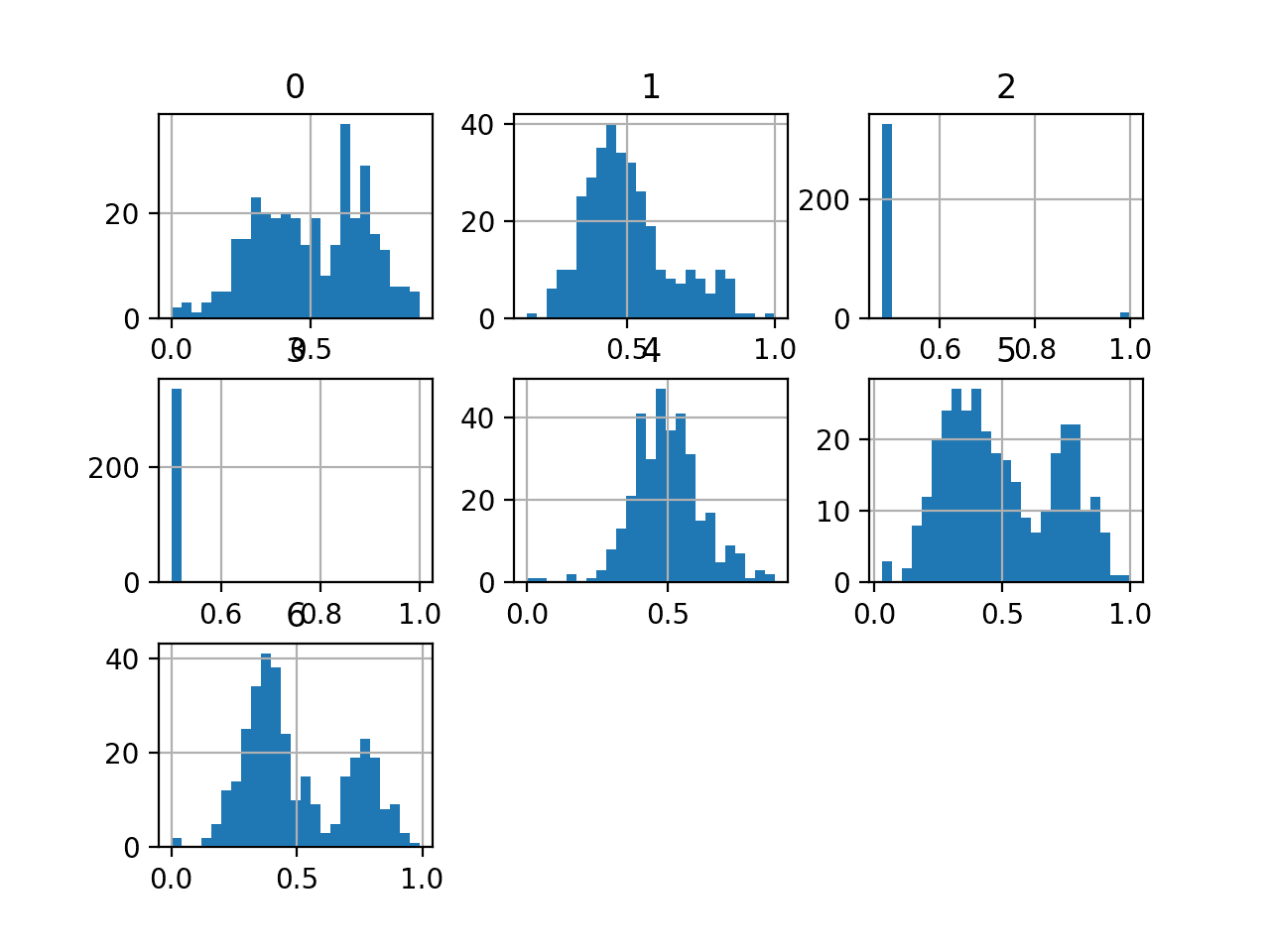
We can also take a look at the distribution of the input variables by creating a histogram for each.

The complete example of creating histograms of all input variables is listed below.

We can see that variables such as 0, 5, and 6 may have a multi-modal distribution. The variables 2 and 3 may have a binary distribution and variables 1 and 4 may have a Gaussian-like distribution.

Depending on the choice of model, the dataset may benefit from standardization, normalization, and perhaps a power transform.

Histogram of Variables in the E.coli Dataset

Now that we have reviewed the dataset, let’s look at developing a test harness for evaluating candidate models.

Model Test and Baseline Result

The k-fold cross-validation procedure provides a good general estimate of model performance that is not too optimistically biased, at least compared to a single train-test split. We will use k=5, meaning each fold will contain about 336/5 or about 67 examples.

Stratified means that each fold will aim to contain the same mixture of examples by class as the entire training dataset. Repeated means that the evaluation process will be performed multiple times to help avoid fluke results and better capture the variance of the chosen model. We will use three repeats.

This means a single model will be fit and evaluated 5 * 3, or 15, times and the mean and standard deviation of these runs will be reported.

This can be achieved using the RepeatedStratifiedKFold scikit-learn class.

All classes are equally important. As such, in this case, we will use classification accuracy to evaluate models.

First, we can define a function to load the dataset and split the input variables into inputs and output variables and use a label encoder to ensure class labels are numbered sequentially.

We can define a function to evaluate a candidate model using stratified repeated 5-fold cross-validation, then return a list of scores calculated on the model for each fold and repeat.

The evaluate_model() function below implements this.

We can then call the load_dataset() function to load and confirm the E.coli dataset.

In this case, we will evaluate the baseline strategy of predicting the majority class in all cases.

This can be implemented automatically using the DummyClassifier class and setting the “strategy” to “most_frequent” that will predict the most common class (e.g. class ‘cp‘) in the training dataset. As such, we would expect this model to achieve a classification accuracy of about 42 percent given this is the distribution of the most common class in the training dataset.

We can then evaluate the model by calling our evaluate_model() function and report the mean and standard deviation of the results.

Tying this all together, the complete example of evaluating the baseline model on the E.coli dataset using classification accuracy is listed below.

Running the example first loads the dataset and reports the number of cases correctly as 336 and the distribution of class labels as we expect.

The DummyClassifier with our default strategy is then evaluated using repeated stratified k-fold cross-validation and the mean and standard deviation of the classification accuracy is reported as about 42.6 percent.

Warnings are reported during the evaluation of the model; for example:

This is because some of the classes do not have a sufficient number of examples for the 5-fold cross-validation, e.g. classes “imS” and “imL“.

In this case, we will remove these examples from the dataset. This can be achieved by updating the load_dataset() to remove those rows with these classes, e.g. four rows.

We can then re-run the example to establish a baseline in classification accuracy.

The complete example is listed below.

Running the example confirms that the number of examples was reduced by four, from 336 to 332.

We can also see that the number of classes was reduced from eight to six (class 0 through to class 5).

The baseline in performance was established at 43.1 percent. This score provides a baseline on this dataset by which all other classification algorithms can be compared. Achieving a score above about 43.1 percent indicates that a model has skill on this dataset, and a score at or below this value indicates that the model does not have skill on this dataset.

Now that we have a test harness and a baseline in performance, we can begin to evaluate some models on this dataset.

Evaluate Models

In this section, we will evaluate a suite of different techniques on the dataset using the test harness developed in the previous section.

The reported performance is good, but not highly optimized (e.g. hyperparameters are not tuned).

Can you do better? If you can achieve better classification accuracy using the same test harness, I’d love to hear about it. Let me know in the comments below.

Evaluate Machine Learning Algorithms

Let’s start by evaluating a mixture of machine learning models on the dataset.

It can be a good idea to spot check a suite of different nonlinear algorithms on a dataset to quickly flush out what works well and deserves further attention, and what doesn’t.

We will evaluate the following machine learning models on the E.coli dataset:

• Linear Discriminant Analysis (LDA)
• Support Vector Machine (SVM)
• Bagged Decision Trees (BAG)
• Random Forest (RF)
• Extra Trees (ET)

We will use mostly default model hyperparameters, with the exception of the number of trees in the ensemble algorithms, which we will set to a reasonable default of 1,000.

We will define each model in turn and add them to a list so that we can evaluate them sequentially. The get_models() function below defines the list of models for evaluation, as well as a list of model short names for plotting the results later.

We can then enumerate the list of models in turn and evaluate each, storing the scores for later evaluation.

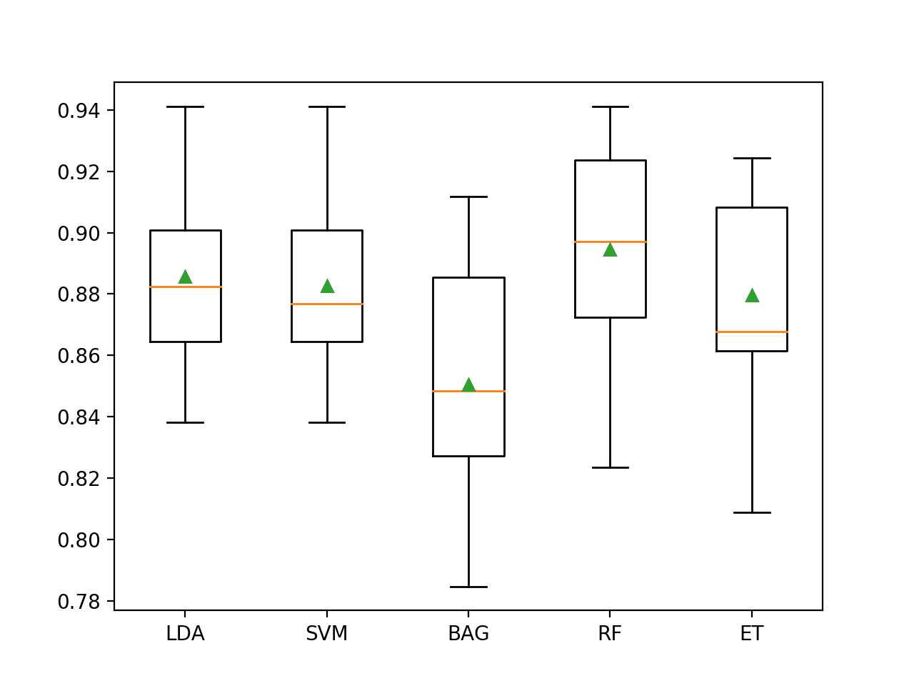
At the end of the run, we can plot each sample of scores as a box and whisker plot with the same scale so that we can directly compare the distributions.

Tying this all together, the complete example of evaluating a suite of machine learning algorithms on the E.coli dataset is listed below.

Running the example evaluates each algorithm in turn and reports the mean and standard deviation classification accuracy.

Note: Your results may vary given the stochastic nature of the algorithm or evaluation procedure, or differences in numerical precision. Consider running the example a few times and compare the average outcome.

In this case, we can see that all of the tested algorithms have skill, achieving an accuracy above the default of 43.1 percent.

The results suggest that most algorithms do well on this dataset and that perhaps the ensembles of decision trees perform the best with Extra Trees achieving 88 percent accuracy and Random Forest achieving 89.5 percent accuracy.

A figure is created showing one box and whisker plot for each algorithm’s sample of results. The box shows the middle 50 percent of the data, the orange line in the middle of each box shows the median of the sample, and the green triangle in each box shows the mean of the sample.

We can see that the distributions of scores for the ensembles of decision trees clustered together separate from the other algorithms tested. In most cases, the mean and median are close on the plot, suggesting a somewhat symmetrical distribution of scores that may indicate the models are stable.

Box and Whisker Plot of Machine Learning Models on the Imbalanced E.coli Dataset

Evaluate Data Oversampling

With so many classes and so few examples in many of the classes, the dataset may benefit from oversampling.

We can test the SMOTE algorithm applied to all except the majority class (cp) results in a lift in performance.

Generally, SMOTE does not appear to help ensembles of decision trees, so we will change the set of algorithms tested to the following:

• Multinomial Logistic Regression (LR)
• Linear Discriminant Analysis (LDA)
• Support Vector Machine (SVM)
• k-Nearest Neighbors (KNN)
• Gaussian Process (GP)

The updated version of the get_models() function to define these models is listed below.

We can use the SMOTE implementation from the imbalanced-learn library, and a Pipeline from the same library to first apply SMOTE to the training dataset, then fit a given model as part of the cross-validation procedure.

SMOTE will synthesize new examples using k-nearest neighbors in the training dataset, where by default, k is set to 5.

This is too large for some of the classes in our dataset. Therefore, we will try a k value of 2.

Tying this together, the complete example of using SMOTE oversampling on the E.coli dataset is listed below.

Running the example evaluates each algorithm in turn and reports the mean and standard deviation classification accuracy.

Note: Your results may vary given the stochastic nature of the algorithm or evaluation procedure, or differences in numerical precision. Consider running the example a few times and compare the average outcome.

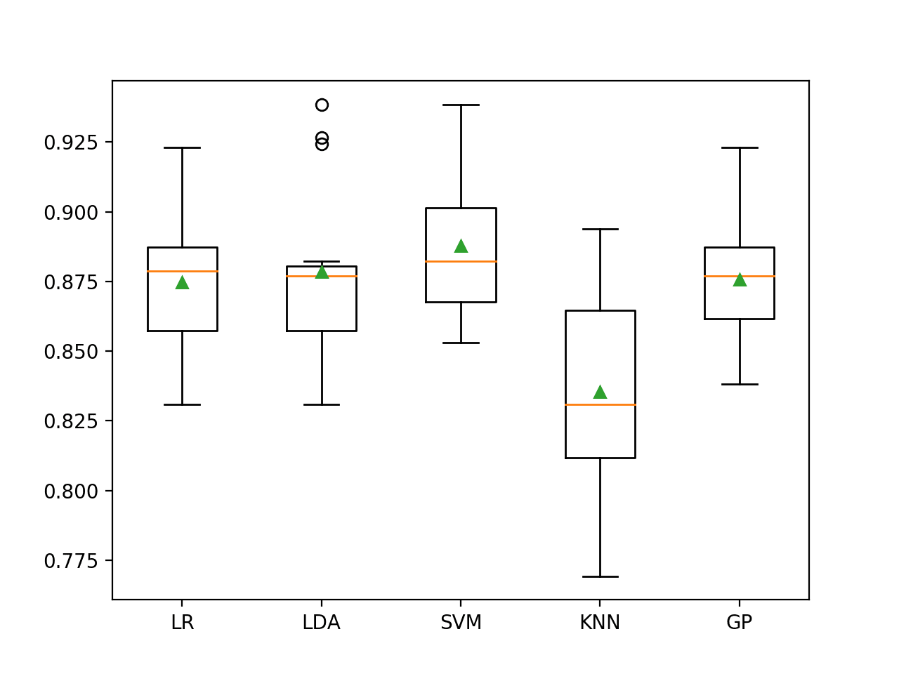
In this case, we can see that LDA with SMOTE resulted in a small drop from 88.6 percent to about 87.9 percent, whereas SVM with SMOTE saw a small increase from about 88.3 percent to about 88.8 percent.

SVM also appears to be the best-performing method when using SMOTE in this case, although it does not achieve an improvement as compared to random forest in the previous section.

Box and whisker plots of classification accuracy scores are created for each algorithm.

We can see that LDA has a number of performance outliers with high 90-percent values, which is quite interesting. It might suggest that LDA could perform better if focused on the abundant classes.

Box and Whisker Plot of SMOTE With Machine Learning Models on the Imbalanced E.coli Dataset

Now that we have seen how to evaluate models on this dataset, let’s look at how we can use a final model to make predictions.

Make Predictions on New Data

In this section, we can fit a final model and use it to make predictions on single rows of data.

We will use the Random Forest model as our final model that achieved a classification accuracy of about 89.5 percent.

First, we can define the model.

Once defined, we can fit it on the entire training dataset.

Once fit, we can use it to make predictions for new data by calling the predict() function. This will return the encoded class label for each example.

We can then use the label encoder to inverse transform to get the string class label.

For example:

To demonstrate this, we can use the fit model to make some predictions of labels for a few cases where we know the outcome.

The complete example is listed below.

Running the example first fits the model on the entire training dataset.

Then the fit model is used to predict the label for one example taken from each of the six classes.

We can see that the correct class label is predicted for each of the chosen examples. Nevertheless, on average, we expect that 1 in 10 predictions will be wrong and these errors may not be equally distributed across the classes.

Further Reading

This section provides more resources on the topic if you are looking to go deeper.

Papers

• Expert System For Predicting Protein Localization Sites In Gram‐negative Bacteria, 1991.
• A Knowledge Base For Predicting Protein Localization Sites In Eukaryotic Cells, 1992.
• A Probabilistic Classification System For Predicting The Cellular Localization Sites Of Proteins, 1996.

APIs

• pandas.read_csv API.
• sklearn.dummy.DummyClassifier API.
• imblearn.over_sampling.SMOTE API.
• imblearn.pipeline.Pipeline API.

Dataset

• Ecoli Dataset, UCI Machine Learning Repository.
• Ecoli Dataset Download.
• Ecoli Dataset Description.

Summary

In this tutorial, you discovered how to develop and evaluate a model for the imbalanced multiclass E.coli dataset.

Specifically, you learned:

• How to load and explore the dataset and generate ideas for data preparation and model selection.
• How to systematically evaluate a suite of machine learning models with a robust test harness.
• How to fit a final model and use it to predict the class labels for specific examples.

Do you have any questions?
Ask your questions in the comments below and I will do my best to answer.

Get a Handle on Imbalanced Classification!

Develop Imbalanced Learning Models in Minutes

...with just a few lines of python code

Discover how in my new Ebook:
Imbalanced Classification with Python

It provides self-study tutorials and end-to-end projects on:
Performance Metrics, Undersampling Methods, SMOTE, Threshold Moving, Probability Calibration, Cost-Sensitive Algorithms
and much more...

Bring Imbalanced Classification Methods to Your Machine Learning Projects

See What's Inside