The PyTorch library is for deep learning. Some applications of deep learning models are used to solve regression or classification problems. In this tutorial, you will discover how to use PyTorch to develop and evaluate neural network models for multi-class classification problems.
After completing this step-by-step tutorial, you will know:
How to load data from CSV and make it available to PyTorch
How to prepare multi-class classification data for modeling with neural networks
How to use cross validation to evaluate a PyTorch neural network model
Kick-start your project with my book Deep Learning with PyTorch. It provides self-study tutorials with working code.
Let’s get started.
Building a multiclass classification model in PyTorch Photo by Cheung Yin. Some rights reserved.
Problem Description
In this tutorial, you will use a standard machine learning dataset called the iris flowers dataset. It is a well-studied dataset and good for practicing machine learning. It has four input variables; all are numeric and length measurements in centimeters. Therefore, they are on a similar scale. Each data sample describes the properties of an observed iris flower. Its goal is to use the measurements (input features) to classify the iris species (output label).
There are three iris species in the dataset. Therefore, it is a multi*class classification problem. Multi-class classification problems are special because they require special handling to specify a class.
This dataset came from Sir Ronald Fisher, the father of modern statistics. It is the best-known dataset for pattern recognition, and you can achieve a model accuracy in the range of 95% to 97%. You can make this your target in developing the deep learning model.
You can download the iris flowers dataset from the UCI Machine Learning repository and place it in your current working directory with the filename “iris.csv“. You can also download the dataset here.
Load the Dataset
There are multiple ways to read a CSV file. The easiest way is probably to use a pandas library. After reading the dataset, you want to split it into features and labels as you need to further process the labels before use. Unlike NumPy or PyTorch tensors, a pandas DataFrame can do slicing by indices only through iloc:
1
2
3
4
import pandas aspd
data=pd.read_csv("iris.csv",header=None)
X=data.iloc[:,0:4]
y=data.iloc[:,4:]
Now, you have loaded the dataset and split the attributes (i.e., input features, columns in the DataFrame) as X and the output variables (i.e., species labels) as a single-column DataFrame y.
Encode the Categorical Variable
The species labels are strings, but you want them in numbers. It is because numerical data are easier to use. In this dataset, the three class labels are Iris-setosa, Iris-versicolor, and Iris-virginica. One way to convert these labels into a number (i.e., encode them) is simply to assign an integer value such as 0, 1, or 2 to replace these labels. But there is a problem: You do not want the model to think that Iris-virginica it is the sum of Iris-setosa and Iris-versicolor. In fact, in statistics, there are levels of measurement:
Nominal numbers: Those numbers are, in fact, names. Operations on them do not make sense
Ordinal numbers: They are orders of something. Comparing for greater or less than makes sense, but addition or subtraction does not
Interval numbers: They are measurements, such as the year today, so that subtraction bears meaning (e.g., how old are you), but the zero value is arbitrary and not special
Ratio numbers: Like interval, but the zero is meaningful, such as the measure of length or time. In this case, both subtraction and division bear meaning, and you can say that something is twice as long.
The encoded label is nominal. You do not want to mistake it as interval or ratio data, but your model would not know. One way to avoid such a mistake is with one-hot encoding, which instead of converting a label into an integer, converts a label into a one-hot vector. A one-hot vector is a vector of integers, but only one of them is 1, and the rest are all zero. In this case, you convert the labels into the following:
1
2
3
Iris-setosa 1 0 0
Iris-versicolor 0 1 0
Iris-virginica 0 0 1
The above is a one-hot encoded binary matrix. You don’t need to create it manually. You can encode the strings consistently to integers using the scikit-learn class LabelEncoder or into one-hot encoding vectors using the class OneHotEncoder:
Then the string labels are transformed into one-hot vectors like the following:
1
2
3
4
5
6
7
[[1.0.0.]
[1.0.0.]
[1.0.0.]
...
[0.0.1.]
[0.0.1.]
[0.0.1.]]
Want to Get Started With Deep Learning with PyTorch?
Take my free email crash course now (with sample code).
Click to sign-up and also get a free PDF Ebook version of the course.
Define the Neural Network Model
Now you need to have a model that can take the input and predict the output, ideally in the form of one-hot vectors. There is no science behind the design of a perfect neural network model. But know one thing–it has to take in a vector of 4 features and output a vector of 3 values. The 4 features correspond to what you have in the dataset. The 3-value output is because we know the one-hot vector has 3 elements. Anything can be in between, known as the “hidden layers,” since they are neither input nor output.
The simplest is to have only one hidden layer. Let’s make one like this:
1
[4 inputs] -> [8 hidden neurons] -> [3 outputs]
Such a design is called the network topology. You should use a “softmax” activation at the output layer. In the formula, it means:
This normalizes the values ($z_1,z_2,z_3$) and applies a non-linear function such that the sum of all 3 outputs will be 1, and each of them is in the range of 0 to 1. This makes the output look like a vector of probabilities. The use of the softmax function at the output is the signature of a multi-class classification model. But in PyTorch, you can skip this if you combine it with an appropriate loss function.
In PyTorch, you can build such a model as follows:
1
2
3
4
5
6
7
8
9
10
11
12
13
14
15
16
import torch
import torch.nn asnn
classMulticlass(nn.Module):
def __init__(self):
super().__init__()
self.hidden=nn.Linear(4,8)
self.act=nn.ReLU()
self.output=nn.Linear(8,3)
def forward(self,x):
x=self.act(self.hidden(x))
x=self.output(x)
returnx
model=Multiclass()
The output of this model is the “weight” of the three classes. Ideally, the model output will be such that only one of the elements is positive infinity, and the rest are negative infinity, making an extreme contrast with absolute confidence to which of the three classes the input features belong. In an imperfect situation, as always happens, you can expect a good model to tell you that one of the values is very positive, and the others are very negative. Or if you transform these values using a sigmoid function or softmax function, one is very close to 1, and the others are very close to 0.
In this case, the loss metric for the output can simply be measuring how close the output is to the one-hot vector you transformed from the label. But usually, in multi-class classification, you use categorical cross entropy as the loss metric. In the formula, it is:
$$
H(p,q) = -\sum_x p(x) \log q(x)
$$
This means, given the real probability vector $p(x)$ and the predicted probability vector $q(x)$, the similarity is the sum of the product of $p(x)$ and $\log q(x)$ for each element $x$. The one-hot vector is considered as the probability vector $p(x)$, and the model output is $q(x)$. Since it is a one-hot vector, only the actual class has $p(x)=1$, and the other classes have $p(x)=0$. The sum above is essentially $-\log q(x)$ of the actual class $x$. The value will be 0 when $q(x)=1$, and as $q(x)$ approaches 0 (the minimum value softmax can produce), $-\log q(x)$ approaches infinity.
Below is how you can define the loss metric. The CrossEntropyLoss function in PyTorch combines the softmax function with the cross entropy calculation, so you don’t need any activation function at the output layer of your model. You also need an optimizer, and Adam is chosen below.
Note that when you define the optimizer, you need to tell it the model parameters as well since these are what the optimizer is going to update.
Now you need to run the training loop to train your model. Minimally, you need to put three steps in the loop: a forward pass, a backward pass, and the weight update. The forward pass provides the input to the model and takes the output. The backward pass starts with the loss metric, which is based on the model output, and propagates the gradient backto the input. The weight update is based on the gradient used to update the weights.
A minimal training loop can be implemented using a for-loop. But you can make use of tqdm to create a progress bar visualization:
1
2
3
4
5
6
7
8
9
10
11
12
13
14
15
16
17
18
19
20
21
22
23
24
25
26
27
import tqdm
# convert pandas DataFrame (X) and numpy array (y) into PyTorch tensors
X=torch.tensor(X.values,dtype=torch.float32)
y=torch.tensor(y,dtype=torch.float32)
# training parameters
n_epochs=200
batch_size=5
batches_per_epoch=len(X)// batch_size
forepoch inrange(n_epochs):
with tqdm.trange(batches_per_epoch,unit="batch",mininterval=0)asbar:
bar.set_description(f"Epoch {epoch}")
foriinbar:
# take a batch
start=i *batch_size
X_batch=X[start:start+batch_size]
y_batch=y[start:start+batch_size]
# forward pass
y_pred=model(X_batch)
loss=loss_fn(y_pred,y_batch)
# backward pass
optimizer.zero_grad()
loss.backward()
# update weights
optimizer.step()
Benchmark the Model
The goal of a model is never to match the dataset per se. The reason you want to build a machine learning model is to prepare for the data you will encounter in the future, which is unseen yet. How can you know the model can do that? You need a test set. It is a dataset that is the same structure as the one used in training but is separate. So it is like unseen data from the training process, and you can take that as a benchmark. This technique of evaluating a model is called cross validation.
Usually, you do not add a test set but split the data set you obtained into a training set and a test set. Then you use the test set to evaluate the model at the end. Such a benchmark serves another purpose: You do not want your model to overfit. It means the model learned too much about the training set and failed to generalize. If this happens, you will see that the model does not give a good result on the test set.
Splitting the data into a training set and a test set can be easily done with scikit-learn. The workflow from loading data to one-hot encoding and splitting is as follows:
1
2
3
4
5
6
7
8
9
10
11
12
13
14
15
16
17
import pandas aspd
from sklearn.model_selection import train_test_split
The arguments train_size=0.7 with shuffle=True means to randomly select 70% of the samples in the dataset into the training set, while the rest will become the test set.
Once you do that, you need to modify the training loop to use the training set in training and use the test set at the end of each epoch for benchmarking:
1
2
3
4
5
6
7
8
9
10
11
12
13
14
15
16
17
18
19
20
21
22
23
24
n_epochs=200
batch_size=5
batches_per_epoch=len(X_train)// batch_size
forepoch inrange(n_epochs):
with tqdm.trange(batches_per_epoch,unit="batch",mininterval=0)asbar:
That’s almost everything you need to finish a deep learning model in PyTorch. But you may also want to do a bit more: Firstly, after all the training epochs, you may want to roll back the model to the best you ever achieved rather than the last one. Secondly, you may want to produce a graph to visualize how the cross entropy and accuracy progressed.
It is not difficult to do. In the training loop, you keep track of the accuracy on the test set and keep a copy of the model whenever this accuracy is higher. And at the same time, remember the metrics you calculated in a list. Then at the end of the training loop, you restore the best model you ever saw and plot the metrics as a time series.
In code, this is how the training loop is modified into:
1
2
3
4
5
6
7
8
9
10
11
12
13
14
15
16
17
18
19
20
21
22
23
24
25
26
27
28
29
30
31
32
33
34
35
36
37
38
39
40
41
42
43
44
45
46
47
48
49
50
51
52
53
54
55
56
57
58
59
60
import copy
import tqdm
import numpy asnp
n_epochs=200
batch_size=5
batches_per_epoch=len(X_train)// batch_size
best_acc=-np.inf# init to negative infinity
best_weights=None
train_loss_hist=[]
train_acc_hist=[]
test_loss_hist=[]
test_acc_hist=[]
forepoch inrange(n_epochs):
epoch_loss=[]
epoch_acc=[]
# set model in training mode and run through each batch
model.train()
with tqdm.trange(batches_per_epoch,unit="batch",mininterval=0)asbar:
You added more lines into the training loop but for a good reason. It is a good practice to switch the model between training mode and evaluation mode when you are switching between the training set and test set. In this particular model, nothing is changed. But for some other models, it will affect the model’s behavior.
You collected metrics in Python lists. You need to be careful to convert the PyTorch tensor (even if it is a scalar value) into a Python float. The purpose of this conversion is to make a copy of the number so that PyTorch will not silently mutate it (e.g., through the optimizer).
After each epoch, you calculated the accuracy based on the test set, and the model weight is stored if you saw the accuracy is higher. However, when you take out the model weight, you should make a deep copy; otherwise, you lost them when the model changes its weights in the next epoch.
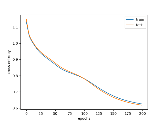
Finally, you can plot the loss and accuracy across epochs using matplotlib as follows:
1
2
3
4
5
6
7
8
9
10
11
12
13
14
15
import matplotlib.pyplot asplt
plt.plot(train_loss_hist,label="train")
plt.plot(test_loss_hist,label="test")
plt.xlabel("epochs")
plt.ylabel("cross entropy")
plt.legend()
plt.show()
plt.plot(train_acc_hist,label="train")
plt.plot(test_acc_hist,label="test")
plt.xlabel("epochs")
plt.ylabel("accuracy")
plt.legend()
plt.show()
A typical result is as follows:
Training and validation loss
Training and validation accuracy
You can see from the graph that at the beginning, both training and test accuracy are very low. This is when your model is underfitting and is performing horribly. As you keep training the model, the accuracy increases, and the cross entropy loss decreases. But at a certain point, the training accuracy is higher than the test accuracy, and in fact, even when the training accuracy improves, the test accuracy flattened or even lowered. This is when the model overfitted, and you do not want to use such a model. That’s why you want to keep track of the test accuracy and restore the model weight to the best result based on the test set.
Complete Example
Putting everything together, the following is the complete code:
1
2
3
4
5
6
7
8
9
10
11
12
13
14
15
16
17
18
19
20
21
22
23
24
25
26
27
28
29
30
31
32
33
34
35
36
37
38
39
40
41
42
43
44
45
46
47
48
49
50
51
52
53
54
55
56
57
58
59
60
61
62
63
64
65
66
67
68
69
70
71
72
73
74
75
76
77
78
79
80
81
82
83
84
85
86
87
88
89
90
91
92
93
94
95
96
97
98
99
100
101
102
103
104
105
106
107
108
109
110
111
112
113
114
115
116
117
import copy
import matplotlib.pyplot asplt
import numpy asnp
import pandas aspd
import torch
import torch.nn asnn
import torch.optim asoptim
import tqdm
from sklearn.model_selection import train_test_split
It provides self-study tutorials with hundreds of working code to turn you from a novice to expert. It equips you with tensor operation, training, evaluation, hyperparameter optimization,
and much more...
Kick-start your deep learning journey with hands-on exercises
Glad you like it. The reason you saw a problem is because of the scikit-learn version you used. In version 1.2, the parameter became sparse_output while the earlier version says sparse.


Hi Adrian:
Nice tutorial. Thank you .
In the line
ohe = OneHotEncoder(handle_unknown=’ignore’, sparse_output=False).fit(y)
the ‘sparse_output’ param does not work for me. I had to change it to ‘sparse’
best
Glad you like it. The reason you saw a problem is because of the scikit-learn version you used. In version 1.2, the parameter became
sparse_outputwhile the earlier version sayssparse.Hi Alberto…You are very welcome! Thank you for the feedback!
How do you make predictions with the trained model?
Hi Juan…The following may be of interest to you:
https://machinelearningmastery.com/how-to-make-classification-and-regression-predictions-for-deep-learning-models-in-keras/
Thank you. I’m a pytorch newbie and your tutorials are easy to understand.
You are welcome Anthony! We are pleased to know that you are making progress with our tutorials.
I got the following error when trying to run the code under Colab (all previous codes up to that point were fine):
File “”, line 3
loss_fn = nn.CrossEntropyLoss()
^
SyntaxError: invalid syntax ^
Hi SFLam…Did you copy and paste the code or type it in?
The potential error lies here:
import torch.optim as optim
loss_fn = nn.CrossEntropyLoss()
optimizer = optim.Adam(model.parameters(), lr=0.001)
Hi, I got the following error when trying to run the code under VS Code.
Epoch 0: : 0batch [00:00, ?batch/s]
Traceback (most recent call last):
88 line ce = loss_fn(y_pred, y_test)
^^^^^^^^^^^^^^^^^^^^^^^
RuntimeError: 0D or 1D target tensor expected, multi-target not supported
Hi kostas…Did you copy and paste the code or type it in? Also, have you tried your code in Google Colab?