PyTorch library is for deep learning. Some applications of deep learning models are to solve regression or classification problems.
In this post, you will discover how to use PyTorch to develop and evaluate neural network models for regression problems.
After completing this post, you will know:
- How to load data from scikit-learn and adapt it for PyTorch models
- How to create a neural network for regerssion problem using PyTorch
- How to improve model performance with data preparation techniques
Kick-start your project with my book Deep Learning with PyTorch. It provides self-study tutorials with working code.
Let’s get started.

Building a Regression Model in PyTorchPhoto by Sam Deng. Some rights reserved.
Description of the Dataset
The dataset you will use in this tutorial is the California housing dataset.
This is a dataset that describes the median house value for California districts. Each data sample is a census block group. The target variable is the median house value in USD 100,000 in 1990 and there are 8 input features, each describing something about the house. They are, namely,
- MedInc: median income in block group
- HouseAge: median house age in block group
- AveRooms: average number of rooms per household
- AveBedrms: average number of bedrooms per household
- Population: block group population
- AveOccup: average number of household members
- Latitude: block group centroid latitude
- Longitude: block group centroid longitude
This data is special because the input data is in vastly different scale. For example, the number of rooms per house is usually small but the population per block group is usually large. Moreover, most features should be positive but the longitude must be negative (because that’s about California). Handling such diversity of data is a challenge to some machine learning models.
You can get the dataset from scikit-learn, which in turn, is downloaded from the Internet at realtime:
|
1 2 3 4 5 6 |
from sklearn.datasets import fetch_california_housing data = fetch_california_housing() print(data.feature_names) X, y = data.data, data.target |
Building a Model and Train
This is a regression problem. Unlike classification problems, the output variable is a continuous value. In case of neural networks, you usually use linear activation at the output layer (i.e., no activation) such that the output range theoretically can be anything from negative infinty to positive infinity.
Also for regression problems, you should never expect the model to predict the values perfectly. Therefore, you should care about how close the prediction is to the actual value. The loss metric that you can use for this is the mean square error (MSE) or mean absolute error (MAE). But you may also interested in the root mean squared error (RMSE) because that’s a metric in the same unit as your output variable.
Let’s try the traditional design of a neural network, namely, the pyramid structure. A pyramid structure is to have the number of neurons in each layer decreasing as the network progresses to the output. The number of input features is fixed, but you set a large number of neurons on the first hidden layer and gradually reduce the number in the subsequent layers. Because you have only one target in this dataset, the final layer should output only one value.
One design is as follows:
|
1 2 3 4 5 6 7 8 9 10 11 12 |
import torch.nn as nn # Define the model model = nn.Sequential( nn.Linear(8, 24), nn.ReLU(), nn.Linear(24, 12), nn.ReLU(), nn.Linear(12, 6), nn.ReLU(), nn.Linear(6, 1) ) |
To train this network, you need to define a loss function. MSE is a reasonable choice. You also need an optimizer, such as Adam.
|
1 2 3 4 5 6 |
import torch.nn as nn import torch.optim as optim # loss function and optimizer loss_fn = nn.MSELoss() # mean square error optimizer = optim.Adam(model.parameters(), lr=0.0001) |
To train this model, you can use your usual training loop. In order to obtain an evaluation score so you are confident that the model works, you need to split the data into training and test sets. You may also want to avoid overfitting by keeping track on the test set MSE. The following is the training loop with the train-test split:
|
1 2 3 4 5 6 7 8 9 10 11 12 13 14 15 16 17 18 19 20 21 22 23 24 25 26 27 28 29 30 31 32 33 34 35 36 37 38 39 40 41 42 43 44 45 46 47 48 49 50 51 52 53 54 |
import copy import numpy as np import torch import tqdm from sklearn.model_selection import train_test_split # train-test split of the dataset X_train, X_test, y_train, y_test = train_test_split(X, y, train_size=0.7, shuffle=True) X_train = torch.tensor(X_train, dtype=torch.float32) y_train = torch.tensor(y_train, dtype=torch.float32).reshape(-1, 1) X_test = torch.tensor(X_test, dtype=torch.float32) y_test = torch.tensor(y_test, dtype=torch.float32).reshape(-1, 1) # training parameters n_epochs = 100 # number of epochs to run batch_size = 10 # size of each batch batch_start = torch.arange(0, len(X_train), batch_size) # Hold the best model best_mse = np.inf # init to infinity best_weights = None history = [] # training loop for epoch in range(n_epochs): model.train() with tqdm.tqdm(batch_start, unit="batch", mininterval=0, disable=True) as bar: bar.set_description(f"Epoch {epoch}") for start in bar: # take a batch X_batch = X_train[start:start+batch_size] y_batch = y_train[start:start+batch_size] # forward pass y_pred = model(X_batch) loss = loss_fn(y_pred, y_batch) # backward pass optimizer.zero_grad() loss.backward() # update weights optimizer.step() # print progress bar.set_postfix(mse=float(loss)) # evaluate accuracy at end of each epoch model.eval() y_pred = model(X_test) mse = loss_fn(y_pred, y_test) mse = float(mse) history.append(mse) if mse < best_mse: best_mse = mse best_weights = copy.deepcopy(model.state_dict()) # restore model and return best accuracy model.load_state_dict(best_weights) |
In the training loop, tqdm is used to set up a progress bar and in each iteration step, MSE is calculated and reported. You can see how the MSE changed by setting the tqdm parameter disable above to False.
Note that in the training loop, each epoch is to run the forward and backward steps with the training set a few times to optimize the model weights, and at the end of the epoch, the model is evaluated using the test set. It is the MSE from the test set that is remembered in the list history. It is also the metric to evaluate a model, which the best one is stored in the variable best_weights.
After you run this, you will have the best model restored and the best MSE stored in the variable best_mse. Note that the mean square error is the average of the square of the difference between the predicted value and the actual value. The square root of it, RMSE, can be regarded as the average difference and it is numerically more useful.
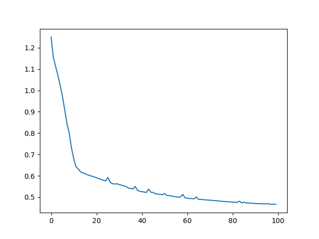
In below, you can show the MSE and RMSE, and plot the history of MSE. It should be decreasing with the epochs.
|
1 2 3 4 |
print("MSE: %.2f" % best_mse) print("RMSE: %.2f" % np.sqrt(best_mse)) plt.plot(history) plt.show() |
This model produced:
|
1 2 |
MSE: 0.47 RMSE: 0.68 |
The MSE graph would like the following.
Putting everything together, the following is the complete code.
|
1 2 3 4 5 6 7 8 9 10 11 12 13 14 15 16 17 18 19 20 21 22 23 24 25 26 27 28 29 30 31 32 33 34 35 36 37 38 39 40 41 42 43 44 45 46 47 48 49 50 51 52 53 54 55 56 57 58 59 60 61 62 63 64 65 66 67 68 69 70 71 72 73 74 75 76 77 78 79 80 81 82 83 |
import copy import matplotlib.pyplot as plt import numpy as np import pandas as pd import torch import torch.nn as nn import torch.optim as optim import tqdm from sklearn.model_selection import train_test_split from sklearn.datasets import fetch_california_housing # Read data data = fetch_california_housing() X, y = data.data, data.target # train-test split for model evaluation X_train, X_test, y_train, y_test = train_test_split(X, y, train_size=0.7, shuffle=True) # Convert to 2D PyTorch tensors X_train = torch.tensor(X_train, dtype=torch.float32) y_train = torch.tensor(y_train, dtype=torch.float32).reshape(-1, 1) X_test = torch.tensor(X_test, dtype=torch.float32) y_test = torch.tensor(y_test, dtype=torch.float32).reshape(-1, 1) # Define the model model = nn.Sequential( nn.Linear(8, 24), nn.ReLU(), nn.Linear(24, 12), nn.ReLU(), nn.Linear(12, 6), nn.ReLU(), nn.Linear(6, 1) ) # loss function and optimizer loss_fn = nn.MSELoss() # mean square error optimizer = optim.Adam(model.parameters(), lr=0.0001) n_epochs = 100 # number of epochs to run batch_size = 10 # size of each batch batch_start = torch.arange(0, len(X_train), batch_size) # Hold the best model best_mse = np.inf # init to infinity best_weights = None history = [] for epoch in range(n_epochs): model.train() with tqdm.tqdm(batch_start, unit="batch", mininterval=0, disable=True) as bar: bar.set_description(f"Epoch {epoch}") for start in bar: # take a batch X_batch = X_train[start:start+batch_size] y_batch = y_train[start:start+batch_size] # forward pass y_pred = model(X_batch) loss = loss_fn(y_pred, y_batch) # backward pass optimizer.zero_grad() loss.backward() # update weights optimizer.step() # print progress bar.set_postfix(mse=float(loss)) # evaluate accuracy at end of each epoch model.eval() y_pred = model(X_test) mse = loss_fn(y_pred, y_test) mse = float(mse) history.append(mse) if mse < best_mse: best_mse = mse best_weights = copy.deepcopy(model.state_dict()) # restore model and return best accuracy model.load_state_dict(best_weights) print("MSE: %.2f" % best_mse) print("RMSE: %.2f" % np.sqrt(best_mse)) plt.plot(history) plt.show() |
Want to Get Started With Deep Learning with PyTorch?
Take my free email crash course now (with sample code).
Click to sign-up and also get a free PDF Ebook version of the course.
Improving the Model with Preprocessing
In the above, you see the RMSE is 0.68. Indeed, it is easy to improve the RMSE by polishing the data before training. The problem of this dataset is the diversity of the features: Some are with a narrow range and some are wide. And some are small but positive while some are very negative. This indeed is not very nice to most of the machine learning model.
One way to improve this is to apply a standard scaler. It is to convert each feature into their standard score. In other words, for each feature $x$, you replace it with
$$
z = \frac{x – \bar{x}}{\sigma_x}
$$
Where $\bar{x}$ is the mean of $x$ and $\sigma_x$ is the standard deviation. This way, every transformed feature is centered around 0 and in a narrow range that around 70% of the samples are between -1 to +1. This can help the machine learning model to converge.
You can apply the standard scaler from scikit-learn. The following is how you should modify the data preparation part of the above code:
|
1 2 3 4 5 6 7 8 9 10 11 12 13 14 15 16 17 18 19 20 21 22 23 |
import torch from sklearn.model_selection import train_test_split from sklearn.datasets import fetch_california_housing from sklearn.preprocessing import StandardScaler # Read data data = fetch_california_housing() X, y = data.data, data.target # train-test split for model evaluation X_train_raw, X_test_raw, y_train, y_test = train_test_split(X, y, train_size=0.7, shuffle=True) # Standardizing data scaler = StandardScaler() scaler.fit(X_train_raw) X_train = scaler.transform(X_train_raw) X_test = scaler.transform(X_test_raw) # Convert to 2D PyTorch tensors X_train = torch.tensor(X_train, dtype=torch.float32) y_train = torch.tensor(y_train, dtype=torch.float32).reshape(-1, 1) X_test = torch.tensor(X_test, dtype=torch.float32) y_test = torch.tensor(y_test, dtype=torch.float32).reshape(-1, 1) |
Note that standard scaler is applied after train-test split. The StandardScaler above is fitted on the training set but applied on both the training and test set. You must not apply the standard scaler to all data because nothing from the test set should be hinted to the model. Otherwise you are introducing data leakage.
Other than that, virtually nothing shall be changed: You still have 8 features (only they are not the same in value). You still use the same training loop. If you train the model with the scaled data, you should see the RMSE improved, e.g.,
|
1 2 |
MSE: 0.29 RMSE: 0.54 |
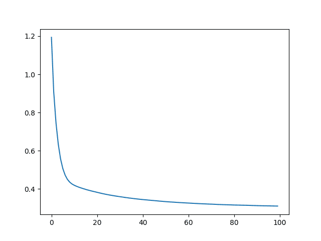
While the MSE history is in a similar falling shape, the y-axis shows it is indeed better after scaling:
However, you need to be careful at the end: When you use the trained model and apply to new data, you should apply the scaler to the input data before feed into the mode. That is, inference should be done as follows:
|
1 2 3 4 5 6 7 8 9 |
model.eval() with torch.no_grad(): # Test out inference with 5 samples from the original test set for i in range(5): X_sample = X_test_raw[i: i+1] X_sample = scaler.transform(X_sample) X_sample = torch.tensor(X_sample, dtype=torch.float32) y_pred = model(X_sample) print(f"{X_test_raw[i]} -> {y_pred[0].numpy()} (expected {y_test[i].numpy()})") |
The following is the complete code:
|
1 2 3 4 5 6 7 8 9 10 11 12 13 14 15 16 17 18 19 20 21 22 23 24 25 26 27 28 29 30 31 32 33 34 35 36 37 38 39 40 41 42 43 44 45 46 47 48 49 50 51 52 53 54 55 56 57 58 59 60 61 62 63 64 65 66 67 68 69 70 71 72 73 74 75 76 77 78 79 80 81 82 83 84 85 86 87 88 89 90 91 92 93 94 95 96 97 98 99 100 |
import copy import matplotlib.pyplot as plt import numpy as np import pandas as pd import torch import torch.nn as nn import torch.optim as optim import tqdm from sklearn.model_selection import train_test_split from sklearn.datasets import fetch_california_housing from sklearn.preprocessing import StandardScaler # Read data data = fetch_california_housing() X, y = data.data, data.target # train-test split for model evaluation X_train_raw, X_test_raw, y_train, y_test = train_test_split(X, y, train_size=0.7, shuffle=True) # Standardizing data scaler = StandardScaler() scaler.fit(X_train_raw) X_train = scaler.transform(X_train_raw) X_test = scaler.transform(X_test_raw) # Convert to 2D PyTorch tensors X_train = torch.tensor(X_train, dtype=torch.float32) y_train = torch.tensor(y_train, dtype=torch.float32).reshape(-1, 1) X_test = torch.tensor(X_test, dtype=torch.float32) y_test = torch.tensor(y_test, dtype=torch.float32).reshape(-1, 1) # Define the model model = nn.Sequential( nn.Linear(8, 24), nn.ReLU(), nn.Linear(24, 12), nn.ReLU(), nn.Linear(12, 6), nn.ReLU(), nn.Linear(6, 1) ) # loss function and optimizer loss_fn = nn.MSELoss() # mean square error optimizer = optim.Adam(model.parameters(), lr=0.0001) n_epochs = 100 # number of epochs to run batch_size = 10 # size of each batch batch_start = torch.arange(0, len(X_train), batch_size) # Hold the best model best_mse = np.inf # init to infinity best_weights = None history = [] for epoch in range(n_epochs): model.train() with tqdm.tqdm(batch_start, unit="batch", mininterval=0, disable=True) as bar: bar.set_description(f"Epoch {epoch}") for start in bar: # take a batch X_batch = X_train[start:start+batch_size] y_batch = y_train[start:start+batch_size] # forward pass y_pred = model(X_batch) loss = loss_fn(y_pred, y_batch) # backward pass optimizer.zero_grad() loss.backward() # update weights optimizer.step() # print progress bar.set_postfix(mse=float(loss)) # evaluate accuracy at end of each epoch model.eval() y_pred = model(X_test) mse = loss_fn(y_pred, y_test) mse = float(mse) history.append(mse) if mse < best_mse: best_mse = mse best_weights = copy.deepcopy(model.state_dict()) # restore model and return best accuracy model.load_state_dict(best_weights) print("MSE: %.2f" % best_mse) print("RMSE: %.2f" % np.sqrt(best_mse)) plt.plot(history) plt.show() model.eval() with torch.no_grad(): # Test out inference with 5 samples for i in range(5): X_sample = X_test_raw[i: i+1] X_sample = scaler.transform(X_sample) X_sample = torch.tensor(X_sample, dtype=torch.float32) y_pred = model(X_sample) print(f"{X_test_raw[i]} -> {y_pred[0].numpy()} (expected {y_test[i].numpy()})") |
Of course, there is still room to imporve the model. One way is to present the target in log scale or, equivalently, use mean absolute percentage error (MAPE) as the loss function. This is because the target variable is the value of houses and it is in a wide range. For the same error magnitude, it is more an issue for low-valued houses. It is your exercise to modify the above code to produce a better prediction.
Summary
In this post, you discovered the use of PyTorch to build a regression model.
You learned how you can work through a regression problem step-by-step with PyTorch, specifically:
- How to load and prepare data for use in PyTorch
- How to create neural network models and choose a loss function for regression
- How to improve model accuracy by applying standard scaler


Re Model Evaluation
Lines 92 and 935 respectfully are:
model.eval()
with torch.no_grad():
# Test out inference with 5 samples
for i in range(5):
And the validation evaluation excludes the code “with torch.no_grad():”
see line 76:
model.eval()
Why is torch.no.grad() used for one section for the evaluation and not the other?
The pytorch discussion website states that the code “with torch.no_grad():” can be used for both.
Hi George…No particular reason or limitation. You should make the portions consistent and let us know what you find.
Hi James,
It’s not how the program is run or when the evaluation is called. That won’t tell me a lot of information.
What you need to know is what the pie torch documentation says rather than rely on how a particular model runs.
Is there a way to turn off the intermediate output while iterating through the epochs? Thanks.
Hello James,
I am writing the Regression Model in PyTorch for multiple inputs and multiple outputs, 1st I did the normalization (transformation) of inputs and outputs, but in the de-normalization stage, my cade is showing the error, can you please help me to debug this?
TypeError: ‘int’ object is not callable
Hi Dimple…While I have not encountered this particular error, the following resource may add clarity on how to address it:
https://www.freecodecamp.org/news/typeerror-int-object-is-not-callable-how-to-fix-in-python/#:~:text=The%20%E2%80%9Cint%20object%20is%20not%20callable%E2%80%9D%20error%20occurs%20when%20you,while%20performing%20a%20mathematical%20operation.
Thanks James.
Could you please give one tutorial for PINNS problem in python using pytorch. I would really appreciate if you could show how to write custom loss functions using one or more outputs of a multi-output neural network.
thank you very much for all your tutorials, they helped me a lot, you are great.
You are very welcome Jorge! We greatly appreciate your support and feedback!
Hi James,
Could you please clarify: what’s the purpose of reshaping y_train and y_test tensors? ( y_test = torch.tensor(y_test, dtype=torch.float32).reshape(-1, 1) )
Hi Nick…The following resource may be of interest to you:
https://discuss.pytorch.org/t/reshape-tensors-your-preserve-variable-information-structure/140300
Thanks James.
I probably should specify my question. I can’t figure out why should we use reshape here:
y_train = torch.tensor(y_train, dtype=torch.float32).reshape(-1, 1)
y_test = torch.tensor(y_test , dtype=torch.float32).reshape(-1, 1)
What’s the sense of transforming torch.Size([14447]) into torch.Size([14447, 1])? How does it help?
Hi Nick…The following may be of interest to you:
https://dzone.com/articles/reshaping-pytorch-tensors