A single-layer neural network, also known as a single-layer perceptron, is the simplest type of neural network. It consists of only one layer of neurons, which are connected to the input layer and the output layer. In case of an image classifier, the input layer would be an image and the output layer would be a class label.
To build an image classifier using a single-layer neural network in PyTorch, you’ll first need to prepare your data. This typically involves loading the images and labels into a PyTorch dataloader, and then splitting the data into training and validation sets. Once your data is prepared, you can define your neural network.
Next, you can use PyTorch’s built-in functions to train the network on your training data and evaluate its performance on your validation data. You’ll also need to pick an optimizer such as stochastic gradient descent (SGD) and a loss function like cross-entropy loss.
Note that a single layer neural network might not be ideal for every task, but it can be good as simple classifier and also can be helpful for you to understand the inner workings of the neural network and to be able to debug it.
So, let’s build our image classifier. In the process you’ll learn:
How to use and preprocess built-in datasets in PyTorch.
How to build and train custom neural networks in PyTorch.
How to build a step-by-step image classifier in PyTorch.
How to make predictions using the trained model in PyTorch.
Let’s get started.
Building an Image Classifier with a Single-Layer Neural Network in PyTorch. Picture by Alex Fung. Some rights reserved.
Overview
This tutorial is in three parts; they are
Preparing the Dataset
Build the Model Architecture
Train the Model
Preparing the Dataset
In this tutorial, you will use the CIFAR-10 dataset. It is a dataset for image classification, consisting of 60,000 color images of 32×32 pixels in 10 classes, with 6,000 images per class. There are 50,000 training images and 10,000 test images. The classes include airplanes, cars, birds, cats, deer, dogs, frogs, horses, ships, and trucks. CIFAR-10 is a popular dataset for machine learning and computer vision research, as it is relatively small and simple, yet challenging enough to require the use of deep learning methods. This dataset can be easily imported into PyTorch library.
If you never downloaded the dataset before, you may see this code show you where the images are downloaded from:
1
2
3
4
Downloading https://www.cs.toronto.edu/~kriz/cifar-10-python.tar.gz to ./data/cifar-10-python.tar.gz
0%| | 0/170498071 [00:00<!--?, ?it/s]
Extracting ./data/cifar-10-python.tar.gz to ./data
Files already downloaded and verified
You specified the root directory where the dataset should be downloaded, and setting train=True to import the training set, and train=False to import the test set. The download=True argument will download the dataset if it’s not already present in the specified root directory.
Building the Neural Network Model
Let’s define a simple neural network SimpleNet that inherits from torch.nn.Module. The network has two fully connected (fc) layers, fc1 and fc2, defined in the __init__ method. The first fully connected layer fc1 takes in the image as input and has 100 hidden neurons. Similarly, the second fully connected layer fc2 has 100 input neurons and num_classes output neurons. The num_classes parameter defaults to 10 as there are 10 classes.
Moreover, the forward method defines the forward pass of the network, where the input x is passed through the layers defined in the __init__ method. The method first reshapes the input tensor x to have a desired shape using the view method. The input then passes through the fully connected layers along with their activation functions and, finally, an output tensor is returned.
Kick-start your project with my book Deep Learning with PyTorch. It provides self-study tutorials with working code.
Here is the code for all explained above.
1
2
# Create the Data object
dataset=Data()
And, write a function to visualize this data, which will also be useful when you train the model later.
1
2
3
4
5
6
7
8
9
10
11
12
13
14
import torch.nn asnn
classSimpleNet(nn.Module):
def __init__(self,num_classes=10):
super(SimpleNet,self).__init__()
self.fc1=nn.Linear(32*32*3,100)# Fully connected layer with 100 hidden neurons
self.fc2=nn.Linear(100,num_classes)# Fully connected layer with num_classes outputs
def forward(self,x):
x=x.view(-1,32*32*3)# reshape the input tensor
x=self.fc1(x)
x=torch.relu(x)
x=self.fc2(x)
returnx
Now, let’s instantiate the model object.
1
2
# Instantiate the model
model=SimpleNet()
Want to Get Started With Deep Learning with PyTorch?
Take my free email crash course now (with sample code).
Click to sign-up and also get a free PDF Ebook version of the course.
Training the Model
You will create two instances of PyTorch’s DataLoader class, for training and testing respectively. In train_loader, you set the batch size at 64 and shuffle the training data randomly by setting shuffle=True.
Then, you will define the functions for cross entropy loss and Adam optimizer for training the model. You set the learning rate at 0.001 for the optimizer.
It is similar for test_loader, except we don’t need to shuffle.
Finally, let’s set a training loop to train our model for a few epochs. You will define some empty lists to store the values of the loss and accuracy metrices for loss and accuracy.
# calculate the average training loss and accuracy
train_loss/=len(train_loader)
train_loss_history.append(train_loss)
train_acc/=len(train_loader.dataset)
train_acc_history.append(train_acc)
# set the model to evaluation mode
model.eval()
with torch.no_grad():
forinputs,labels intest_loader:
outputs=model(inputs)
loss=criterion(outputs,labels)
val_loss+=loss.item()
val_acc+=(outputs.argmax(1)==labels).sum().item()
# calculate the average validation loss and accuracy
val_loss/=len(test_loader)
val_loss_history.append(val_loss)
val_acc/=len(test_loader.dataset)
val_acc_history.append(val_acc)
print(f'Epoch {epoch+1}/{num_epochs}, train loss: {train_loss:.4f}, train acc: {train_acc:.4f}, val loss: {val_loss:.4f}, val acc: {val_acc:.4f}')
Running this loop will print you the following:
1
2
3
4
5
6
7
8
9
10
11
12
13
14
15
16
17
18
19
20
Epoch 1/20, train loss: 1.8757, train acc: 0.3292, val loss: 1.7515, val acc: 0.3807
Epoch 2/20, train loss: 1.7254, train acc: 0.3862, val loss: 1.6850, val acc: 0.4008
Epoch 3/20, train loss: 1.6548, train acc: 0.4124, val loss: 1.6692, val acc: 0.3987
Epoch 4/20, train loss: 1.6150, train acc: 0.4268, val loss: 1.6052, val acc: 0.4265
Epoch 5/20, train loss: 1.5874, train acc: 0.4343, val loss: 1.5803, val acc: 0.4384
Epoch 6/20, train loss: 1.5598, train acc: 0.4424, val loss: 1.5928, val acc: 0.4315
Epoch 7/20, train loss: 1.5424, train acc: 0.4506, val loss: 1.5489, val acc: 0.4514
Epoch 8/20, train loss: 1.5310, train acc: 0.4568, val loss: 1.5566, val acc: 0.4454
Epoch 9/20, train loss: 1.5116, train acc: 0.4626, val loss: 1.5501, val acc: 0.4442
Epoch 10/20, train loss: 1.5005, train acc: 0.4677, val loss: 1.5282, val acc: 0.4598
Epoch 11/20, train loss: 1.4911, train acc: 0.4702, val loss: 1.5310, val acc: 0.4629
Epoch 12/20, train loss: 1.4804, train acc: 0.4756, val loss: 1.5555, val acc: 0.4457
Epoch 13/20, train loss: 1.4743, train acc: 0.4762, val loss: 1.5207, val acc: 0.4629
Epoch 14/20, train loss: 1.4658, train acc: 0.4792, val loss: 1.5177, val acc: 0.4570
Epoch 15/20, train loss: 1.4608, train acc: 0.4819, val loss: 1.5529, val acc: 0.4527
Epoch 16/20, train loss: 1.4539, train acc: 0.4832, val loss: 1.5066, val acc: 0.4645
Epoch 17/20, train loss: 1.4486, train acc: 0.4863, val loss: 1.4874, val acc: 0.4727
Epoch 18/20, train loss: 1.4503, train acc: 0.4866, val loss: 1.5318, val acc: 0.4575
Epoch 19/20, train loss: 1.4383, train acc: 0.4910, val loss: 1.5065, val acc: 0.4673
Epoch 20/20, train loss: 1.4348, train acc: 0.4897, val loss: 1.5127, val acc: 0.4679
As you can see, the single-layer classifier is trained for only 20 epochs and it achieved a validation accuracy of around 47 percent. Train it for more epochs and you may get a decent accuracy. Similarly, our model had only a single layer with 100 hidden neurons. If you add some more layers, the accuracy may significantly improve.
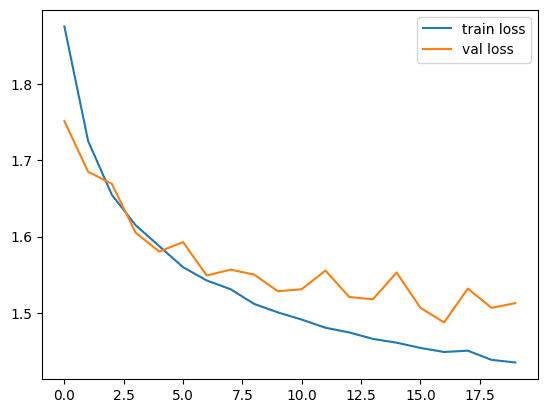
Now, let’s plot loss and accuracy matrices to see how they look like.
1
2
3
4
5
6
7
8
9
10
11
12
13
import matplotlib.pyplot asplt
# Plot the training and validation loss
plt.plot(train_loss_history,label='train loss')
plt.plot(val_loss_history,label='val loss')
plt.legend()
plt.show()
# Plot the training and validation accuracy
plt.plot(train_acc_history,label='train acc')
plt.plot(val_acc_history,label='val acc')
plt.legend()
plt.show()
The loss plot is like:And the accuracy plot is the following:
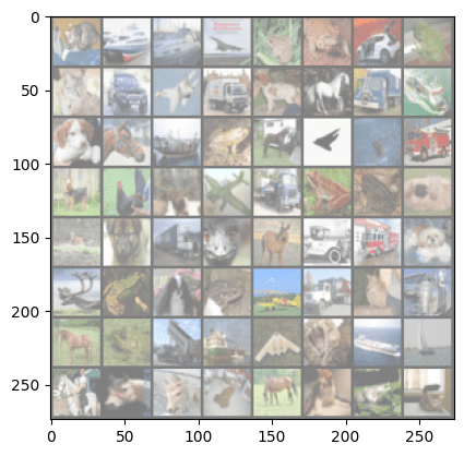
Here is how you can see how the model make predictions against the true labels.
1
2
3
4
5
6
7
8
9
10
11
12
13
14
15
16
17
18
import numpy asnp
# get some validation data
forinputs,labels intest_loader:
break# this line stops the loop after the first iteration
It provides self-study tutorials with hundreds of working code to turn you from a novice to expert. It equips you with tensor operation, training, evaluation, hyperparameter optimization,
and much more...
Kick-start your deep learning journey with hands-on exercises
Model worked but the codes after this i.e.,
plottiungs for accuracy/loss and prediction image,
the kernal died with this message –
‘The kernel appears to have died. It will restart automatically’. I tried several times but the result were same. Any suggestion for solving this? Thanmks.
part was left in the code by mistake? I doesn’t seemed to be used anywhere in the code below it, and the Data() method is never defined prior to its use.
Even single neural network layers don’t scale well with width.
If the width is n then the number of multiply add operations required is n squared.
What starts off as something reasonable at say n=8 giving 64 multiply adds, starts to get unreasonable at n=256 giving 65536 multiply adds.
However by using a combining algorithm you can restrain the costs: https://ai462qqq.blogspot.com/2023/03/switch-net-4-reducing-cost-of-neural.html

 And the accuracy plot is the following:
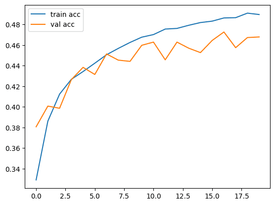


Where is Jason, please?
Model worked but the codes after this i.e.,
plottiungs for accuracy/loss and prediction image,
the kernal died with this message –
‘The kernel appears to have died. It will restart automatically’. I tried several times but the result were same. Any suggestion for solving this? Thanmks.
Hi Chuck…While we have not experienced this issue, the following resource may be helpful:
https://stackoverflow.com/questions/47022997/jupyter-the-kernel-appears-to-have-died-it-will-restart-automatically
# Create the Data object
“dataset = Data()”
Pytorch reported Error after this. The Data Class was not created?
Hi Leo…Please elaborate on your question so that we may better assist you. That is…what errors are you receiving?
in this tutorial it must have been missed, but it was present in other tutorials
use this before dataset = Data():
# Creating the dataset class
class Data(Dataset):
def __init__(self):
self.x = torch.arange(-2, 2, 0.1).view(-1, 1)
self.y = torch.zeros(self.x.shape[0], 1)
self.y[self.x[:, 0] > 0.2] = 1
self.len = self.x.shape[0]
def __getitem__(self, idx):
return self.x[idx], self.y[idx]
def __len__(self):
return self.len
Thank you Fabio for your feedback and suggestion!
Hi,
I think the
dataset = Data()
part was left in the code by mistake? I doesn’t seemed to be used anywhere in the code below it, and the Data() method is never defined prior to its use.
Hi Narae…Thanks for the feedback!
Hi Kames,
Thank yuo for replying
The code and error are here:
————————————————-
import torch
import torchvision
import torchvision.transforms as transforms
# import the CIFAR-10 dataset
train_set = torchvision.datasets.CIFAR10(root=’./data’, train=True, download=True, transform=transforms.ToTensor())
test_set = torchvision.datasets.CIFAR10(root=’./data’, train=False, download=True, transform=transforms.ToTensor())
# Create the Data object
dataset = Data()
————————————————————–
NameError Traceback (most recent call last)
Input In [1], in ()
7 test_set = torchvision.datasets.CIFAR10(root=’./data’, train=False, download=True, transform=transforms.ToTensor())
9 # Create the Data object
—> 10 dataset = Data()
NameError: name ‘Data’ is not defined
Even single neural network layers don’t scale well with width.
If the width is n then the number of multiply add operations required is n squared.
What starts off as something reasonable at say n=8 giving 64 multiply adds, starts to get unreasonable at n=256 giving 65536 multiply adds.
However by using a combining algorithm you can restrain the costs:
https://ai462qqq.blogspot.com/2023/03/switch-net-4-reducing-cost-of-neural.html
Thank you for your feedback and contribution Sean!