Multiclass classification problems are those where a label must be predicted, but there are more than two labels that may be predicted.
These are challenging predictive modeling problems because a sufficiently representative number of examples of each class is required for a model to learn the problem. It is made challenging when the number of examples in each class is imbalanced, or skewed toward one or a few of the classes with very few examples of other classes.
Problems of this type are referred to as imbalanced multiclass classification problems and they require both the careful design of an evaluation metric and test harness and choice of machine learning models. The glass identification dataset is a standard dataset for exploring the challenge of imbalanced multiclass classification.
In this tutorial, you will discover how to develop and evaluate a model for the imbalanced multiclass glass identification dataset.
After completing this tutorial, you will know:
How to load and explore the dataset and generate ideas for data preparation and model selection.
How to systematically evaluate a suite of machine learning models with a robust test harness.
How to fit a final model and use it to predict the class labels for specific examples.
Kick-start your project with my new book Imbalanced Classification with Python, including step-by-step tutorials and the Python source code files for all examples.
Let’s get started.
Update Jun/2020: Added an example that achieves better performance.
Evaluate Models for the Imbalanced Multiclass Glass Identification Dataset Photo by Sarah Nichols, some rights reserved.
Tutorial Overview
This tutorial is divided into five parts; they are:
Glass Identification Dataset
Explore the Dataset
Model Test and Baseline Result
Evaluate Models
Evaluate Machine Learning Algorithms
Improved Models (new)
Make Predictions on New Data
Glass Identification Dataset
In this project, we will use a standard imbalanced machine learning dataset referred to as the “Glass Identification” dataset, or simply “glass.”
The dataset describes the chemical properties of glass and involves classifying samples of glass using their chemical properties as one of six classes. The dataset was credited to Vina Spiehler in 1987.
Ignoring the sample identification number, there are nine input variables that summarize the properties of the glass dataset; they are:
RI: refractive index
Na: Sodium
Mg: Magnesium
Al: Aluminum
Si: Silicon
K: Potassium
Ca: Calcium
Ba: Barium
Fe: Iron
The chemical compositions are measured as the weight percent in corresponding oxide.
There are seven types of glass listed; they are:
Class 1: building windows (float processed)
Class 2: building windows (non-float processed)
Class 3: vehicle windows (float processed)
Class 4: vehicle windows (non-float processed)
Class 5: containers
Class 6: tableware
Class 7: headlamps
Float glass refers to the process used to make the glass.
There are 214 observations in the dataset and the number of observations in each class is imbalanced. Note that there are no examples for class 4 (non-float processed vehicle windows) in the dataset.
Class 1: 70 examples
Class 2: 76 examples
Class 3: 17 examples
Class 4: 0 examples
Class 5: 13 examples
Class 6: 9 examples
Class 7: 29 examples
Although there are minority classes, all classes are equally important in this prediction problem.
The dataset can be divided into window glass (classes 1-4) and non-window glass (classes 5-7). There are 163 examples of window glass and 51 examples of non-window glass.
Window Glass: 163 examples
Non-Window Glass: 51 examples
Another division of the observations would be between float processed glass and non-float processed glass, in the case of window glass only. This division is more balanced.
Float Glass: 87 examples
Non-Float Glass: 76 examples
Next, let’s take a closer look at the data.
Want to Get Started With Imbalance Classification?
Take my free 7-day email crash course now (with sample code).
Click to sign-up and also get a free PDF Ebook version of the course.
Explore the Dataset
First, download the dataset and save it in your current working directory with the name “glass.csv“.
Note that this version of the dataset has the first column (row) number removed as it does not contain generalizable information for modeling.
We can see that the input variables are numeric and the class label is an integer is in the final column.
All of the chemical input variables have the same units, although the first variable, the refractive index, has different units. As such, data scaling may be required for some modeling algorithms.
The dataset can be loaded as a DataFrame using the read_csv() Pandas function, specifying the location of the dataset and the fact that there is no header line.
1
2
3
4
5
...
# define the dataset location
filename='glass.csv'
# load the csv file as a data frame
dataframe=read_csv(filename,header=None)
Once loaded, we can summarize the number of rows and columns by printing the shape of the DataFrame.
1
2
3
...
# summarize the shape of the dataset
print(dataframe.shape)
We can also summarize the number of examples in each class using the Counter object.
Running the example first loads the dataset and confirms the number of rows and columns, which are 214 rows and 9 input variables and 1 target variable.
The class distribution is then summarized, confirming the severe skew in the observations for each class.
1
2
3
4
5
6
7
(214, 10)
Class=1, Count=70, Percentage=32.710%
Class=2, Count=76, Percentage=35.514%
Class=3, Count=17, Percentage=7.944%
Class=5, Count=13, Percentage=6.075%
Class=6, Count=9, Percentage=4.206%
Class=7, Count=29, Percentage=13.551%
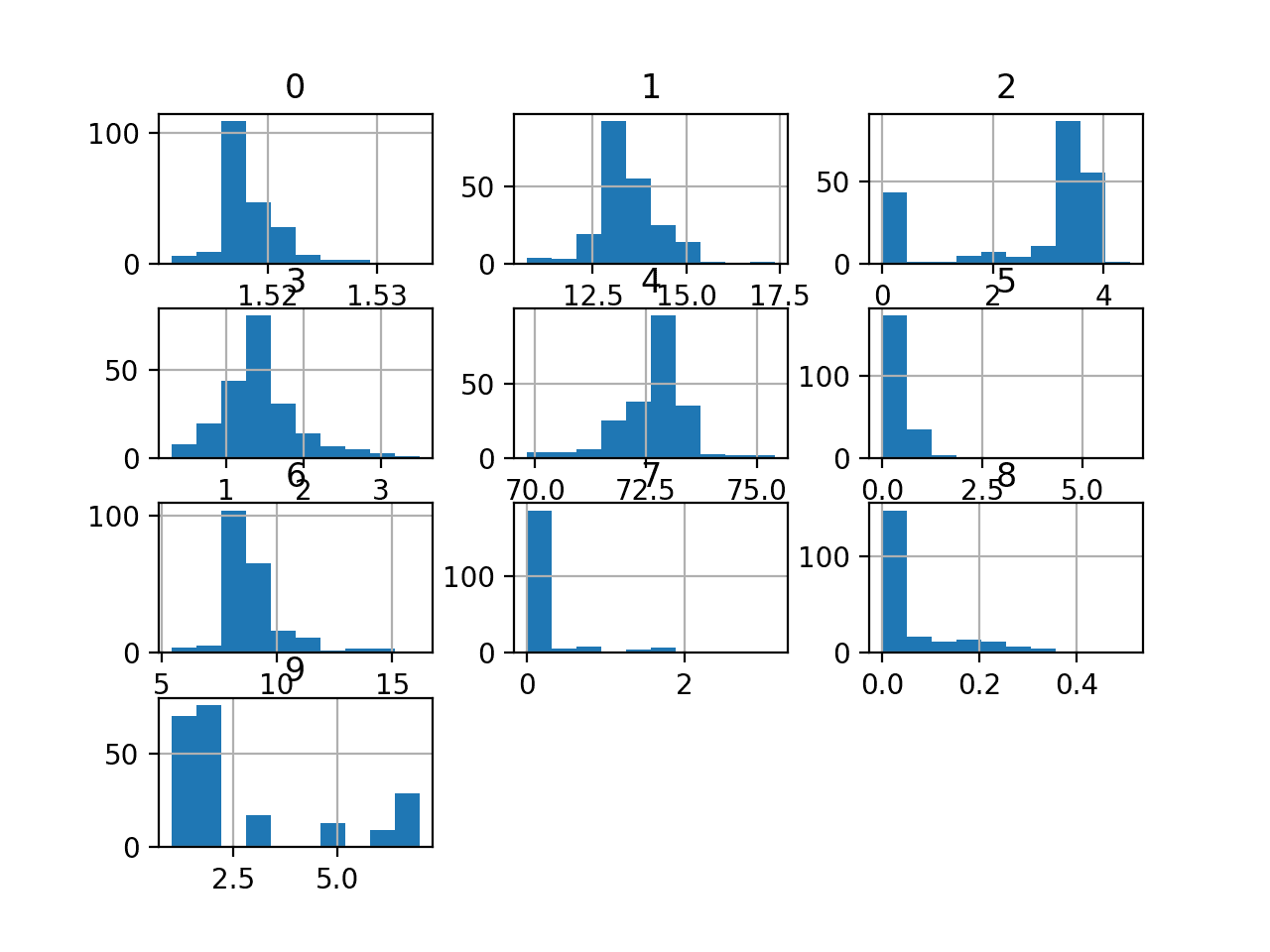
We can also take a look at the distribution of the input variables by creating a histogram for each.
The complete example of creating histograms of all variables is listed below.
1
2
3
4
5
6
7
8
9
10
11
# create histograms of all variables
from pandas import read_csv
from matplotlib import pyplot
# define the dataset location
filename='glass.csv'
# load the csv file as a data frame
df=read_csv(filename,header=None)
# create a histogram plot of each variable
df.hist()
# show the plot
pyplot.show()
We can see that some of the variables have a Gaussian-like distribution and others appear to have an exponential or even a bimodal distribution.
Depending on the choice of algorithm, the data may benefit from standardization of some variables and perhaps a power transform.
Histogram of Variables in the Glass Identification Dataset
Now that we have reviewed the dataset, let’s look at developing a test harness for evaluating candidate models.
Model Test and Baseline Result
We will evaluate candidate models using repeated stratified k-fold cross-validation.
The k-fold cross-validation procedure provides a good general estimate of model performance that is not too optimistically biased, at least compared to a single train-test split. We will use k=5, meaning each fold will contain about 214/5, or about 42 examples.
Stratified means that each fold will aim to contain the same mixture of examples by class as the entire training dataset. Repeated means that the evaluation process will be performed multiple times to help avoid fluke results and better capture the variance of the chosen model. We will use three repeats.
This means a single model will be fit and evaluated 5 * 3 or 15 times and the mean and standard deviation of these runs will be reported.
All classes are equally important. There are minority classes that are only represented with 4 percent or 6 percent of the data, yet no class has more than about 35 percent dominance of the dataset.
As such, in this case, we will use classification accuracy to evaluate models.
First, we can define a function to load the dataset and split the input variables into inputs and output variables and use a label encoder to ensure class labels are numbered sequentially from 0 to 5.
1
2
3
4
5
6
7
8
9
10
11
# load the dataset
def load_dataset(full_path):
# load the dataset as a numpy array
data=read_csv(full_path,header=None)
# retrieve numpy array
data=data.values
# split into input and output elements
X,y=data[:,:-1],data[:,-1]
# label encode the target variable to have the classes 0 and 1
y=LabelEncoder().fit_transform(y)
returnX,y
We can define a function to evaluate a candidate model using stratified repeated 5-fold cross-validation then return a list of scores calculated on the model for each fold and repeat. The evaluate_model() function below implements this.
We can then call the load_dataset() function to load and confirm the glass identification dataset.
1
2
3
4
5
6
7
...
# define the location of the dataset
full_path='glass.csv'
# load the dataset
X,y=load_dataset(full_path)
# summarize the loaded dataset
print(X.shape,y.shape,Counter(y))
In this case, we will evaluate the baseline strategy of predicting the majority class in all cases.
This can be implemented automatically using the DummyClassifier class and setting the “strategy” to “most_frequent” that will predict the most common class (e.g. class 2) in the training dataset.
As such, we would expect this model to achieve a classification accuracy of about 35 percent given this is the distribution of the most common class in the training dataset.
1
2
3
...
# define the reference model
model=DummyClassifier(strategy='most_frequent')
We can then evaluate the model by calling our evaluate_model() function and report the mean and standard deviation of the results.
Tying this all together, the complete example of evaluating the baseline model on the glass identification dataset using classification accuracy is listed below.
1
2
3
4
5
6
7
8
9
10
11
12
13
14
15
16
17
18
19
20
21
22
23
24
25
26
27
28
29
30
31
32
33
34
35
36
37
38
39
40
41
42
# baseline model and test harness for the glass identification dataset
from collections import Counter
from numpy import mean
from numpy import std
from pandas import read_csv
from sklearn.preprocessing import LabelEncoder
from sklearn.model_selection import cross_val_score
from sklearn.model_selection import RepeatedStratifiedKFold
from sklearn.dummy import DummyClassifier
# load the dataset
def load_dataset(full_path):
# load the dataset as a numpy array
data=read_csv(full_path,header=None)
# retrieve numpy array
data=data.values
# split into input and output elements
X,y=data[:,:-1],data[:,-1]
# label encode the target variable to have the classes 0 and 1
Running the example first loads the dataset and reports the number of cases correctly as 214 and the distribution of class labels as we expect.
The DummyClassifier with our default strategy is then evaluated using repeated stratified k-fold cross-validation and the mean and standard deviation of the classification accuracy is reported as about 35.5 percent.
This score provides a baseline on this dataset by which all other classification algorithms can be compared. Achieving a score above about 35.5 percent indicates that a model has skill on this dataset, and a score at or below this value indicates that the model does not have skill on this dataset.
Now that we have a test harness and a baseline in performance, we can begin to evaluate some models on this dataset.
Evaluate Models
In this section, we will evaluate a suite of different techniques on the dataset using the test harness developed in the previous section.
The reported performance is good, but not highly optimized (e.g. hyperparameters are not tuned).
Can you do better? If you can achieve better classification accuracy using the same test harness, I’d love to hear about it. Let me know in the comments below.
Evaluate Machine Learning Algorithms
Let’s evaluate a mixture of machine learning models on the dataset.
It can be a good idea to spot check a suite of different nonlinear algorithms on a dataset to quickly flush out what works well and deserves further attention and what doesn’t.
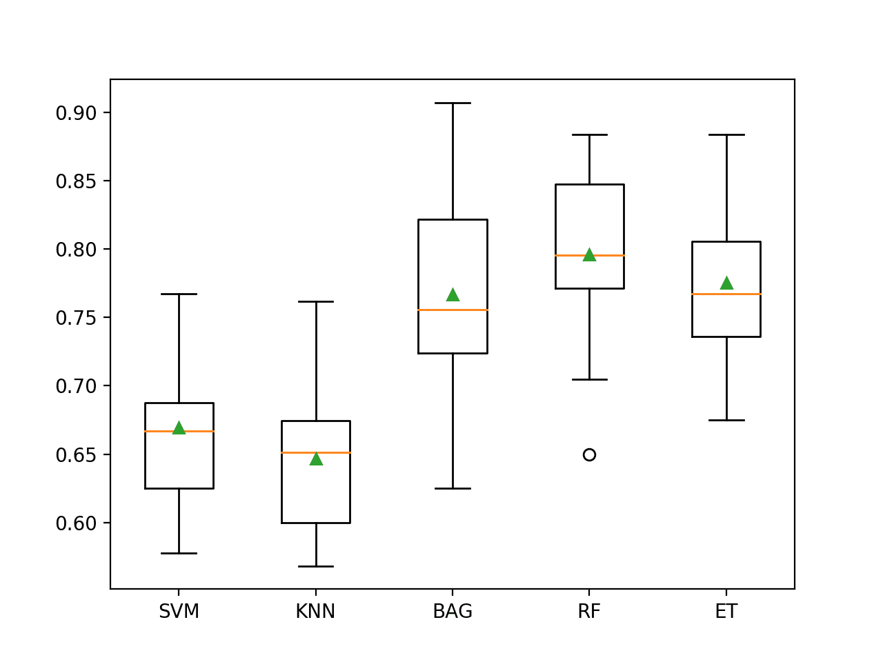
We will evaluate the following machine learning models on the glass dataset:
Support Vector Machine (SVM)
k-Nearest Neighbors (KNN)
Bagged Decision Trees (BAG)
Random Forest (RF)
Extra Trees (ET)
We will use mostly default model hyperparameters, with the exception of the number of trees in the ensemble algorithms, which we will set to a reasonable default of 1,000.
We will define each model in turn and add them to a list so that we can evaluate them sequentially. The get_models() function below defines the list of models for evaluation, as well as a list of model short names for plotting the results later.
At the end of the run, we can plot each sample of scores as a box and whisker plot with the same scale so that we can directly compare the distributions.
Tying this all together, the complete example of evaluating a suite of machine learning algorithms on the glass identification dataset is listed below.
1
2
3
4
5
6
7
8
9
10
11
12
13
14
15
16
17
18
19
20
21
22
23
24
25
26
27
28
29
30
31
32
33
34
35
36
37
38
39
40
41
42
43
44
45
46
47
48
49
50
51
52
53
54
55
56
57
58
59
60
61
62
63
64
65
66
67
68
69
70
71
# spot check machine learning algorithms on the glass identification dataset
from numpy import mean
from numpy import std
from pandas import read_csv
from matplotlib import pyplot
from sklearn.preprocessing import LabelEncoder
from sklearn.model_selection import cross_val_score
from sklearn.model_selection import RepeatedStratifiedKFold
from sklearn.svm import SVC
from sklearn.neighbors import KNeighborsClassifier
from sklearn.ensemble import RandomForestClassifier
from sklearn.ensemble import ExtraTreesClassifier
from sklearn.ensemble import BaggingClassifier
# load the dataset
def load_dataset(full_path):
# load the dataset as a numpy array
data=read_csv(full_path,header=None)
# retrieve numpy array
data=data.values
# split into input and output elements
X,y=data[:,:-1],data[:,-1]
# label encode the target variable to have the classes 0 and 1
Running the example evaluates each algorithm in turn and reports the mean and standard deviation classification accuracy.
Note: Your results may vary given the stochastic nature of the algorithm or evaluation procedure, or differences in numerical precision. Consider running the example a few times and compare the average outcome.
In this case, we can see that all of the tested algorithms have skill, achieving an accuracy above the default of 35.5 percent.
The results suggest that ensembles of decision trees perform well on this dataset, with perhaps random forest performing the best overall achieving a classification accuracy of approximately 79.6 percent.
1
2
3
4
5
>SVM 0.669 (0.057)
>KNN 0.647 (0.055)
>BAG 0.767 (0.070)
>RF 0.796 (0.062)
>ET 0.776 (0.057)
A figure is created showing one box and whisker plot for each algorithm’s sample of results. The box shows the middle 50 percent of the data, the orange line in the middle of each box shows the median of the sample, and the green triangle in each box shows the mean of the sample.
We can see that the distributions of scores for the ensembles of decision trees clustered together separate from the other algorithms tested. In most cases, the mean and median are close on the plot, suggesting a somewhat symmetrical distribution of scores that may indicate the models are stable.
Box and Whisker Plot of Machine Learning Models on the Imbalanced Glass Identification Dataset
Now that we have seen how to evaluate models on this dataset, let’s look at how we can use a final model to make predictions.
Improved Models
This section lists models discovered to have even better performance than those listed above, added after the tutorial was published.
Cost-Sensitive Random Forest (80.8%)
A cost-sensitive version of random forest with custom class weightings was found to achieve better performance.
1
2
3
4
5
6
7
8
9
10
11
12
13
14
15
16
17
18
19
20
21
22
23
24
25
26
27
28
29
30
31
32
33
34
35
36
37
38
39
40
# cost sensitive random forest with custom class weightings
from numpy import mean
from numpy import std
from pandas import read_csv
from sklearn.preprocessing import LabelEncoder
from sklearn.model_selection import cross_val_score
from sklearn.model_selection import RepeatedStratifiedKFold
from sklearn.ensemble import RandomForestClassifier
Running the example evaluates the algorithms and reports the mean and standard deviation accuracy.
Note: Your results may vary given the stochastic nature of the algorithm or evaluation procedure, or differences in numerical precision. Consider running the example a few times and compare the average outcome.
In this case, the model achieves an accuracy of about 80.8%.
1
Mean Accuracy: 0.808 (0.059)
Can you do better? Let me know in the comments below and I will add your model here if I can reproduce the result using the same test harness.
Make Predictions on New Data
In this section, we can fit a final model and use it to make predictions on single rows of data.
We will use the Random Forest model as our final model that achieved a classification accuracy of about 79 percent.
First, we can define the model.
1
2
3
...
# define model to evaluate
model=RandomForestClassifier(n_estimators=1000)
Once defined, we can fit it on the entire training dataset.
1
2
3
...
# fit the model
model.fit(X,y)
Once fit, we can use it to make predictions for new data by calling the predict() function.
This will return the class label for each example.
For example:
1
2
3
4
5
...
# define a row of data
row=[...]
# predict the class label
yhat=model.predict([row])
To demonstrate this, we can use the fit model to make some predictions of labels for a few cases where we know the outcome.
The complete example is listed below.
1
2
3
4
5
6
7
8
9
10
11
12
13
14
15
16
17
18
19
20
21
22
23
24
25
26
27
28
29
30
31
32
33
34
35
36
37
38
39
40
41
42
43
# fit a model and make predictions for the on the glass identification dataset
from pandas import read_csv
from sklearn.preprocessing import LabelEncoder
from sklearn.ensemble import RandomForestClassifier
# load the dataset
def load_dataset(full_path):
# load the dataset as a numpy array
data=read_csv(full_path,header=None)
# retrieve numpy array
data=data.values
# split into input and output elements
X,y=data[:,:-1],data[:,-1]
# label encode the target variable to have the classes 0 and 1
Running the example first fits the model on the entire training dataset.
Then the fit model is used to predict the label for one example taken from each of the six classes.
We can see that the correct class label is predicted for each of the chosen examples. Nevertheless, on average, we expect that 1 in 5 predictions will be wrong and these errors may not be equally distributed across the classes.
1
2
3
4
5
6
>Predicted=0 (expected 0)
>Predicted=1 (expected 1)
>Predicted=2 (expected 2)
>Predicted=3 (expected 3)
>Predicted=4 (expected 4)
>Predicted=5 (expected 5)
Further Reading
This section provides more resources on the topic if you are looking to go deeper.
It provides self-study tutorials and end-to-end projects on: Performance Metrics, Undersampling Methods, SMOTE, Threshold Moving, Probability Calibration, Cost-Sensitive Algorithms
and much more...
Bring Imbalanced Classification Methods to Your Machine Learning Projects
Excellent post.
You did not tell how to handle the imbalanced situation?
What are the most popular packages to use?
Does ensemble models are good by default to handle imbalanced data?
And most importantly, which one have I do first: feature selection or data balancing?
Thanks for sharing, very useful to beginners to see how you begin and how you move along every project. In many projects I see similar steps, but that’s how it is. Thanks!
In multiclass classifications on imbalanced datasets, accuracy is not a valid measure and we should calculate precision, recall, and f1 score too.
I have trained a multiclass and multi task binary network for 35 human attributes. In prediction time, for most classes it always returns 0 or 1. The accuracy is very good, but other measures are really bad. Do you know what could be the problem? I have changed the loss function and added some layers to the resnet50, but the problem persists.
Is linear separability applicable for multi class classification?
If it is applicable, how can I check the linear separability for multi class datasets?
Is it correct if I simply use Logistic Regression fit it on the entire dataset & test it on the entire dataset. Then if I get a score close to 100%, assuming as the classes are linearly separable.
Thanks. Actually I thought of using Logistic Regression only to check linear separability. Not for generating predictions. So in that case will the above mentioned approach work?
According to what I found in stack overflow says:
First of all to check if data is linearly separable do not use cross validation. Just fit your model to entire data and check the error, there is no need for train/validation/test splits, train on everything – test on everything.
From
According to what I found in a blog it is the,
• Accuracy that could be achieved by always predicting the most frequent class.
• This means that a dumb model that always predicts 0/1 would be right “null_accuracy” % of the time.
In your articles you have mentioned it as ‘baseline performance’. I hope that, both the null accuracy & baseline performance are the same.
To calculate this, which set do we have to use from the train & test set?


great post . a good service to learners as well as practitioners.
Thanks!
Excellent post.
You did not tell how to handle the imbalanced situation?
What are the most popular packages to use?
Does ensemble models are good by default to handle imbalanced data?
And most importantly, which one have I do first: feature selection or data balancing?
Thank you.
Good questions, see this framework:
https://machinelearningmastery.com/framework-for-imbalanced-classification-projects/
Thanks for sharing, very useful to beginners to see how you begin and how you move along every project. In many projects I see similar steps, but that’s how it is. Thanks!
I’m happy it helps.
Hi, thanks for your great tutorial.
In multiclass classifications on imbalanced datasets, accuracy is not a valid measure and we should calculate precision, recall, and f1 score too.
I have trained a multiclass and multi task binary network for 35 human attributes. In prediction time, for most classes it always returns 0 or 1. The accuracy is very good, but other measures are really bad. Do you know what could be the problem? I have changed the loss function and added some layers to the resnet50, but the problem persists.
It can be.
I recommend choosing a metric that best captures the goals of your project:
https://machinelearningmastery.com/tour-of-evaluation-metrics-for-imbalanced-classification/
Hi Jason. Do you have an idea on how to make a prediction using multiple rows for this imbalance classification? 🙁
Yes, call model.predict() to make a prediction with one or multiple rows.
Is linear separability applicable for multi class classification?
If it is applicable, how can I check the linear separability for multi class datasets?
Is it correct if I simply use Logistic Regression fit it on the entire dataset & test it on the entire dataset. Then if I get a score close to 100%, assuming as the classes are linearly separable.
Yes.
Perhaps pair-wise plots of data colored by class label.
No, to estimate performance fit on one dataset and evaluate on a different dataset, or use k-fold cross-validation.
Thanks. Actually I thought of using Logistic Regression only to check linear separability. Not for generating predictions. So in that case will the above mentioned approach work?
According to what I found in stack overflow says:
First of all to check if data is linearly separable do not use cross validation. Just fit your model to entire data and check the error, there is no need for train/validation/test splits, train on everything – test on everything.
From
Thanks
San
Maybe.
If a linear model does well on a classification dataset it gives some weak evidence that the dataset is linearly separable.
To calculate the null accuracy, which set do we have to use from the train & test set?
Thanks
San
What is a null accuracy?
According to what I found in a blog it is the,
• Accuracy that could be achieved by always predicting the most frequent class.
• This means that a dumb model that always predicts 0/1 would be right “null_accuracy” % of the time.
In your articles you have mentioned it as ‘baseline performance’. I hope that, both the null accuracy & baseline performance are the same.
To calculate this, which set do we have to use from the train & test set?
Thanks, I have never heard that before.
Different metrics use different naive classifiers, this tutorial will suggest which naive classifier to use for each metric:
https://machinelearningmastery.com/naive-classifiers-imbalanced-classification-metrics/
Suppose I have a train set & a test set as X_train, y_train, X_test, y_test.
I have a multi class classification problem & is it correct if I calculate the train & test error like this?
print(“Train Error “, 1 – accuracy_score( y_train, model.predict( X_train )))
print(“Test Error “, 1 – accuracy_score( y_test, model.predict( X_test )))
Sure, but accuracy is a terrible metric for imbalanced classification:
https://machinelearningmastery.com/failure-of-accuracy-for-imbalanced-class-distributions/
If I use f1_score as the metric, does it make sense if I get the train error & test error like this
print(“Train Error “, 1 – f1_score( y_train, model.predict( X_train )))
print(“Test Error “, 1 – f1_score( y_test, model.predict( X_test )))
Thanks
San
No, that is not valid. Error is the inverse of accuracy as you had it, it is just a poor metric for evaluating imbalanced datasets.
Before applying one hot encoding my features are categorical & after applying OHE, some of those variables become integers.
So what is the correct method for finding the correlation between features, is it before or after applying one hot encoding?
Thanks
San
Correlation is calculated on raw data, not one hot encoded data.
Categorical correlation for categorical data, numerical correlation for numerical data:
https://machinelearningmastery.com/feature-selection-with-real-and-categorical-data/
Hello Jason. I have a dataset with a total amount of data reaching 3000. The dataset is divided into several classes.
class A: 455
Class B: 540
class C: 566
class D: 491
class E: 399
class F: 248
class G: 450
class H: 295
What I want to ask is whether the dataset I have is an imbalanced dataset?
Thank you for your help
I little bit imbalanced. Try this framework:
https://machinelearningmastery.com/framework-for-imbalanced-classification-projects/
Hi Jason. I am beginner in machine learning. My imbalanced dataset is divided to four classes and total amount of 3000 instances:
class A: 0
class B: 1802
class C: 1198
class D: 0
how can I predict classes with precision in this dataset? I would be grateful if you guided me through this.
This tutorial will show you how to configure precision for multi-class classification:
https://machinelearningmastery.com/precision-recall-and-f-measure-for-imbalanced-classification/
Hello sir,
The blog was just awesome.
One thing I couldn’t understand is how did you choose the weights for the Random Forest?
Are there any rules?
Thank you
Thanks.
Set to “balanced” and it will set the weights for you based on the dataset.