Fraud is a major problem for credit card companies, both because of the large volume of transactions that are completed each day and because many fraudulent transactions look a lot like normal transactions.
Identifying fraudulent credit card transactions is a common type of imbalanced binary classification where the focus is on the positive class (is fraud) class.
As such, metrics like precision and recall can be used to summarize model performance in terms of class labels and precision-recall curves can be used to summarize model performance across a range of probability thresholds when mapping predicted probabilities to class labels.
This gives the operator of the model control over how predictions are made in terms of biasing toward false positive or false negative type errors made by the model.
In this tutorial, you will discover how to develop and evaluate a model for the imbalanced credit card fraud dataset.
After completing this tutorial, you will know:
How to load and explore the dataset and generate ideas for data preparation and model selection.
How to systematically evaluate a suite of machine learning models with a robust test harness.
How to fit a final model and use it to predict the probability of fraud for specific cases.
Let’s get started.
How to Predict the Probability of Fraudulent Credit Card Transactions Photo by Andrea Schaffer, some rights reserved.
Tutorial Overview
This tutorial is divided into five parts; they are:
Credit Card Fraud Dataset
Explore the Dataset
Model Test and Baseline Result
Evaluate Models
Make Predictions on New Data
Credit Card Fraud Dataset
In this project, we will use a standard imbalanced machine learning dataset referred to as the “Credit Card Fraud Detection” dataset.
The data represents credit card transactions that occurred over two days in September 2013 by European cardholders.
All details of the cardholders have been anonymized via a principal component analysis (PCA) transform. Instead, a total of 28 principal components of these anonymized features is provided. In addition, the time in seconds between transactions is provided, as is the purchase amount (presumably in Euros).
Each record is classified as normal (class “0”) or fraudulent (class “1” ) and the transactions are heavily skewed towards normal. Specifically, there are 492 fraudulent credit card transactions out of a total of 284,807 transactions, which is a total of about 0.172% of all transactions.
It contains a subset of online transactions that occurred in two days, where we have 492 frauds out of 284,807 transactions. The dataset is highly unbalanced, where the positive class (frauds) account for 0.172% of all transactions …
Some publications use the ROC area under curve metric, although the website for the dataset recommends using the precision-recall area under curve metric, given the severe class imbalance.
Given the class imbalance ratio, we recommend measuring the accuracy using the Area Under the Precision-Recall Curve (AUPRC).
Note that this version of the dataset has the header line removed. If you download the dataset from Kaggle, you must remove the header line first.
We can see that the first column is the time, which is an integer, and the second last column is the purchase amount. The final column contains the class label. We can see that the PCA transformed features are positive and negative and contain a lot of floating point precision.
The time column is unlikely to be useful and probably can be removed. The difference in scale between the PCA variables and the dollar amount suggests that data scaling should be used for those algorithms that are sensitive to the scale of input variables.
The dataset can be loaded as a DataFrame using the read_csv() Pandas function, specifying the location and the names of the columns, as there is no header line.
1
2
3
4
5
...
# define the dataset location
filename='creditcard.csv'
# load the csv file as a data frame
dataframe=read_csv(filename,header=None)
Once loaded, we can summarize the number of rows and columns by printing the shape of the DataFrame.
1
2
3
...
# summarize the shape of the dataset
print(dataframe.shape)
We can also summarize the number of examples in each class using the Counter object.
Running the example first loads the dataset and confirms the number of rows and columns, which are 284,807 rows and 30 input variables and 1 target variable.
The class distribution is then summarized, confirming the severe skew in the class distribution, with about 99.827 percent of transactions marked as normal and about 0.173 percent marked as fraudulent. This generally matches the description of the dataset in the paper.
1
2
3
(284807, 31)
Class=0, Count=284315, Percentage=99.827%
Class=1, Count=492, Percentage=0.173%
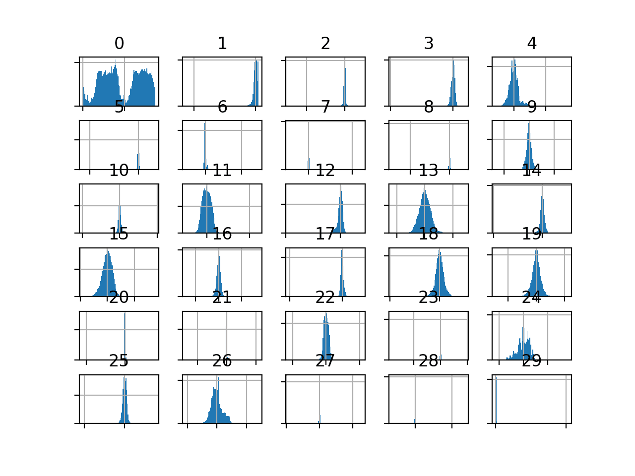
We can also take a look at the distribution of the input variables by creating a histogram for each.
Because of the large number of variables, the plots can look cluttered. Therefore we will disable the axis labels so that we can focus on the histograms. We will also increase the number of bins used in each histogram to help better see the data distribution.
The complete example of creating histograms of all input variables is listed below.
1
2
3
4
5
6
7
8
9
10
11
12
13
14
15
16
17
# create histograms of input variables
from pandas import read_csv
from matplotlib import pyplot
# define the dataset location
filename='creditcard.csv'
# load the csv file as a data frame
df=read_csv(filename,header=None)
# drop the target variable
df=df.drop(30,axis=1)
# create a histogram plot of each numeric variable
ax=df.hist(bins=100)
# disable axis labels to avoid the clutter
foraxis inax.flatten():
axis.set_xticklabels([])
axis.set_yticklabels([])
# show the plot
pyplot.show()
We can see that the distribution of most of the PCA components is Gaussian, and many may be centered around zero, suggesting that the variables were standardized as part of the PCA transform.
Histogram of Input Variables in the Credit Card Fraud Dataset
The amount variable might be interesting and does not appear on the histogram.
This suggests that the distribution of the amount values may be skewed. We can create a 5-number summary of this variable to get a better idea of the transaction sizes.
The complete example is listed below.
1
2
3
4
5
6
7
8
# summarize the amount variable
from pandas import read_csv
# define the dataset location
filename='creditcard.csv'
# load the csv file as a data frame
df=read_csv(filename,header=None)
# summarize the amount variable.
print(df[29].describe())
Running the example, we can see that most amounts are small, with a mean of about 88 and the middle 50 percent of observations between 5 and 77.
The largest value is about 25,691, which is pulling the distribution up and might be an outlier (e.g. someone purchased a car on their credit card).
1
2
3
4
5
6
7
8
9
count 284807.000000
mean 88.349619
std 250.120109
min 0.000000
25% 5.600000
50% 22.000000
75% 77.165000
max 25691.160000
Name: 29, dtype: float64
Now that we have reviewed the dataset, let’s look at developing a test harness for evaluating candidate models.
Model Test and Baseline Result
We will evaluate candidate models using repeated stratified k-fold cross-validation.
The k-fold cross-validation procedure provides a good general estimate of model performance that is not too optimistically biased, at least compared to a single train-test split. We will use k=10, meaning each fold will contain about 284807/10 or 28,480 examples.
Stratified means that each fold will contain the same mixture of examples by class, that is about 99.8 percent to 0.2 percent normal and fraudulent transaction respectively. Repeated means that the evaluation process will be performed multiple times to help avoid fluke results and better capture the variance of the chosen model. We will use 3 repeats.
This means a single model will be fit and evaluated 10 * 3 or 30 times and the mean and standard deviation of these runs will be reported.
We will use the recommended metric of area under precision-recall curve or PR AUC.
This requires that a given algorithm first predict a probability or probability-like measure. The predicted probabilities are then evaluated using precision and recall at a range of different thresholds for mapping probability to class labels, and the area under the curve of these thresholds is reported as the performance of the model.
This metric focuses on the positive class, which is desirable for such a severe class imbalance. It also allows the operator of a final model to choose a threshold for mapping probabilities to class labels (fraud or non-fraud transactions) that best balances the precision and recall of the final model.
We can define a function to load the dataset and split the columns into input and output variables. The load_dataset() function below implements this.
1
2
3
4
5
6
7
8
9
# load the dataset
def load_dataset(full_path):
# load the dataset as a numpy array
data=read_csv(full_path,header=None)
# retrieve numpy array
data=data.values
# split into input and output elements
X,y=data[:,:-1],data[:,-1]
returnX,y
We can then define a function that will calculate the precision-recall area under curve for a given set of predictions.
This involves first calculating the precision-recall curve for the predictions via the precision_recall_curve() function. The output recall and precision values for each threshold can then be provided as arguments to the auc() to calculate the area under the curve. The pr_auc() function below implements this.
1
2
3
4
5
6
# calculate precision-recall area under curve
def pr_auc(y_true,probas_pred):
# calculate precision-recall curve
p,r,_=precision_recall_curve(y_true,probas_pred)
# calculate area under curve
returnauc(r,p)
We can then define a function that will evaluate a given model on the dataset and return a list of PR AUC scores for each fold and repeat.
The evaluate_model() function below implements this, taking the dataset and model as arguments and returning the list of scores. The make_scorer() function is used to define the precision-recall AUC metric and indicates that a model must predict probabilities in order to be evaluated.
Finally, we can evaluate a baseline model on the dataset using this test harness.
A model that predicts the positive class (class 1) for all examples will provide a baseline performance when using the precision-recall area under curve metric.
This can be achieved using the DummyClassifier class from the scikit-learn library and setting the “strategy” argument to ‘constant‘ and setting the “constant” argument to ‘1’ to predict the positive class.
Running the example first loads and summarizes the dataset.
We can see that we have the correct number of rows loaded and that we have 30 input variables.
Next, the average of the PR AUC scores is reported.
In this case, we can see that the baseline algorithm achieves a mean PR AUC of about 0.501.
This score provides a lower limit on model skill; any model that achieves an average PR AUC above about 0.5 has skill, whereas models that achieve a score below this value do not have skill on this dataset.
Now that we have a test harness and a baseline in performance, we can begin to evaluate some models on this dataset.
Evaluate Models
In this section, we will evaluate a suite of different techniques on the dataset using the test harness developed in the previous section.
The goal is to both demonstrate how to work through the problem systematically and to demonstrate the capability of some techniques designed for imbalanced classification problems.
The reported performance is good but not highly optimized (e.g. hyperparameters are not tuned).
Can you do better? If you can achieve better PR AUC performance using the same test harness, I’d love to hear about it. Let me know in the comments below.
Evaluate Machine Learning Algorithms
Let’s start by evaluating a mixture of machine learning models on the dataset.
It can be a good idea to spot check a suite of different nonlinear algorithms on a dataset to quickly flush out what works well and deserves further attention and what doesn’t.
We will evaluate the following machine learning models on the credit card fraud dataset:
Decision Tree (CART)
k-Nearest Neighbors (KNN)
Bagged Decision Trees (BAG)
Random Forest (RF)
Extra Trees (ET)
We will use mostly default model hyperparameters, with the exception of the number of trees in the ensemble algorithms, which we will set to a reasonable default of 100. We will also standardize the input variables prior to providing them as input to the KNN algorithm.
We will define each model in turn and add them to a list so that we can evaluate them sequentially. The get_models() function below defines the list of models for evaluation, as well as a list of model short names for plotting the results later.
At the end of the run, we can plot each sample of scores as a box and whisker plot with the same scale so that we can directly compare the distributions.
Tying this all together, the complete example of an evaluation of a suite of machine learning algorithms on the credit card fraud dataset is listed below.
1
2
3
4
5
6
7
8
9
10
11
12
13
14
15
16
17
18
19
20
21
22
23
24
25
26
27
28
29
30
31
32
33
34
35
36
37
38
39
40
41
42
43
44
45
46
47
48
49
50
51
52
53
54
55
56
57
58
59
60
61
62
63
64
65
66
67
68
69
70
71
72
73
74
75
76
77
78
79
80
81
82
83
# spot check machine learning algorithms on the credit card fraud dataset
from numpy import mean
from numpy import std
from pandas import read_csv
from matplotlib import pyplot
from sklearn.preprocessing import StandardScaler
from sklearn.pipeline import Pipeline
from sklearn.model_selection import cross_val_score
from sklearn.model_selection import RepeatedStratifiedKFold
from sklearn.metrics import precision_recall_curve
from sklearn.metrics import auc
from sklearn.metrics import make_scorer
from sklearn.tree import DecisionTreeClassifier
from sklearn.neighbors import KNeighborsClassifier
from sklearn.ensemble import RandomForestClassifier
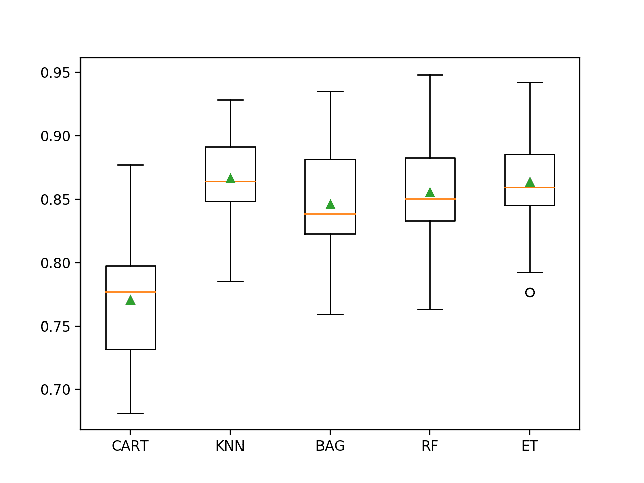
Running the example evaluates each algorithm in turn and reports the mean and standard deviation PR AUC.
Note: Your results may vary given the stochastic nature of the algorithm or evaluation procedure, or differences in numerical precision. Consider running the example a few times and compare the average outcome.
In this case, we can see that all of the tested algorithms have skill, achieving a PR AUC above the default of 0.5. The results suggest that the ensembles of decision tree algorithms all do well on this dataset, although the KNN with standardization of the dataset seems to perform the best on average.
1
2
3
4
5
>CART 0.771 (0.049)
>KNN 0.867 (0.033)
>BAG 0.846 (0.045)
>RF 0.855 (0.046)
>ET 0.864 (0.040)
A figure is created showing one box and whisker plot for each algorithm’s sample of results. The box shows the middle 50 percent of the data, the orange line in the middle of each box shows the median of the sample, and the green triangle in each box shows the mean of the sample.
We can see that the distributions of scores for the KNN and ensembles of decision trees are tight and means seem to coincide with medians, suggesting the distributions may be symmetrical and are probably Gaussian and that the scores are probably quite stable.
Box and Whisker Plot of Machine Learning Models on the Imbalanced Credit Card Fraud Dataset
Now that we have seen how to evaluate models on this dataset, let’s look at how we can use a final model to make predictions.
Make Prediction on New Data
In this section, we can fit a final model and use it to make predictions on single rows of data.
We will use the KNN model as our final model that achieved a PR AUC of about 0.867. Fitting the final model involves defining a Pipeline to scale the numerical variables prior to fitting the model.
The Pipeline can then be used to make predictions on new data directly and will automatically scale new data using the same operations as performed on the training dataset.
Running the example first fits the model on the entire training dataset.
Then the fit model is used to predict the label of normal cases chosen from the dataset file. We can see that all cases are correctly predicted.
Then some fraud cases are used as input to the model and the label is predicted. As we might have hoped, most of the examples are predicted correctly with the default threshold. This highlights the need for a user of the model to select an appropriate probability threshold.
Normal cases:
1
2
3
4
5
6
7
>Predicted=0.000 (expected 0)
>Predicted=0.000 (expected 0)
>Predicted=0.000 (expected 0)
Fraud cases:
>Predicted=1.000 (expected 1)
>Predicted=0.400 (expected 1)
>Predicted=1.000 (expected 1)
Further Reading
This section provides more resources on the topic if you are looking to go deeper.
It provides self-study tutorials and end-to-end projects on: Performance Metrics, Undersampling Methods, SMOTE, Threshold Moving, Probability Calibration, Cost-Sensitive Algorithms
and much more...
Bring Imbalanced Classification Methods to Your Machine Learning Projects
Jason:
Although my SKFold PR AUC scores generally follow yours: KNN 0.869 (0.042), ET 0.862 (0.043), RF (with balanced class weight) 0.858 (0.046), both RF and ET outperfomed KNN when employed on a 80/20 train/test of the dataset. RF achieved PR AUC score of 0.845 and a Recall score on the fraud class of 0.75 (with 0.94 Precision); ET achieved PR AUC score of 0.838 and also a Recall score of 0.75 (with 0.93 Precision). By comparison, KNN achieved PR AUC score of 0.807and a Recall score of 0.69 (with 0.92 Precision). It is surprising to me that these three models essentially performed equivalently on this dataset.
Hi Jason, nice article!
I’m having trouble understanding how the DummyClassifier can bring a PR AUC of 0.501. It should have a fixed recall of 100% and precision of .2%, whatever the threshold. Am I missing something here?
Thank you Jason for this succinct and well explained post. I would like to ask a question, as to why no under sampling or oversampling was performed as the data is skewed with very less fraud transactions. Thank you!!
I have got much better results in simple way from most of the algorithms .
by svm= 99.93504441557529
by random_forest = 99.96137776061234
by decision tree = 99.92275552122467
by knn= 99.95611109160492
by logistic regression = 99.91748885221726
by Gradient Boosting Classifier = 99.77177767634564
me too..
I train with 100% data of the dataset and test with the same data, I got above 99% accuracy. however, when I try to split 50% data for training and 50% for testing, the result was very terrible.
Can you please make a blog post on anomaly detection for a data without any prior labels? Also, if you have resources, please point me to streaming anomaly detection implementations. Thanks a lot.
Quick question – Why are we using the strategy as ‘constant’ where as it should be ‘stratified’ for PR-AUC metric? Am I missing something here?
I think you mentioned this in one of you posts:
“Predicting a constant value, like the majority class or minority class will result in an invalid PR Curve (e.g. a point) and in turn an invalid PR AUC score. Scores for models that predict a constant value should be ignored”
Hi Jason, nice article!
I have learned a lot from you! Very useful articles.
There’s a problem, I think when you predict on unlabeled datasets, the number of false positives will be so much, I don’t see you mention this.
The reason I say that is because I’m working on a spam call prediction project, my dataset is similar to yours.
Perhaps you need an alternate data prep/model/model config?
Perhaps the test harness you used to evaluate your model was not reliable? E.g. try repeated stratified 10-fold cv?
Very informative post! At the end of the article you mention that it is up to the user to make an appropriate probability threshold in order to predict the positive class. I was wondering if there was a way to find the optimal threshold? Or is it more by trial and error?
Hi Robert…You do raise an interesting question! I am not aware of any method to establish an optimal threshold, however you could gather sufficient historical data and determine a most likely threshold based upon statistical methods.
Hello. When should we apply oversampling or undersampling techniques and when should we continue working with the unbalanced data set? Thank you very much for all the information you share on your blogs.


Hi Jason, very good article as always. Don’t you think the results would have been better if you used class_weights on your models ?
Thanks.
Try it, see if you can get better results.
Hi Jason, very usful tutor! Please, help to adapt pr_auc and evaluate_model functions for the case of multiclass (few classes) classification.
Thanks for the suggestion.
really wonderful, thank you
Thanks!
Jason:
Although my SKFold PR AUC scores generally follow yours: KNN 0.869 (0.042), ET 0.862 (0.043), RF (with balanced class weight) 0.858 (0.046), both RF and ET outperfomed KNN when employed on a 80/20 train/test of the dataset. RF achieved PR AUC score of 0.845 and a Recall score on the fraud class of 0.75 (with 0.94 Precision); ET achieved PR AUC score of 0.838 and also a Recall score of 0.75 (with 0.93 Precision). By comparison, KNN achieved PR AUC score of 0.807and a Recall score of 0.69 (with 0.92 Precision). It is surprising to me that these three models essentially performed equivalently on this dataset.
Nice work!
Thanks.
Another nice dataset to work with is the data brick Auto Insurance Claim Fraud Detection set: https://databricks-prod-cloudfront.cloud.databricks.com/public/4027ec902e239c93eaaa8714f173bcfc/4954928053318020/1058911316420443/167703932442645/latest.html
Recall Scores above 0.950 can be achieved using LR, ET, or RF together with SMOTEENN. Ron
Thanks for sharing.
Hi Jason, Here you didn’t seem to use Cost sensitive algorithm that you discussed in earlier post. Is there any idea or strategy for not using here?
Yes, I used an appropriate metric, then I could not achieve better performance than using standard models with that metric.
If you can do better on the same test harness, please share your results.
Hi Jason, nice article!
I’m having trouble understanding how the DummyClassifier can bring a PR AUC of 0.501. It should have a fixed recall of 100% and precision of .2%, whatever the threshold. Am I missing something here?
Thanks
This may help:
https://machinelearningmastery.com/naive-classifiers-imbalanced-classification-metrics/
For more research works related to this topic refer to https://www.researchgate.net/project/Fraud-detection-with-machine-learning
Thanks for sharing.
Thank you Jason for this succinct and well explained post. I would like to ask a question, as to why no under sampling or oversampling was performed as the data is skewed with very less fraud transactions. Thank you!!
You’re welcome.
It did not help on this problem.
I have got much better results in simple way from most of the algorithms .
by svm= 99.93504441557529
by random_forest = 99.96137776061234
by decision tree = 99.92275552122467
by knn= 99.95611109160492
by logistic regression = 99.91748885221726
by Gradient Boosting Classifier = 99.77177767634564
Wow, did you use the same evaluation procedure as above?
me too..
I train with 100% data of the dataset and test with the same data, I got above 99% accuracy. however, when I try to split 50% data for training and 50% for testing, the result was very terrible.
Perhaps use repeated k-fold cross-validation to estimate model performance instead of a simple train/test split.
Hi Jason,
Can you please make a blog post on anomaly detection for a data without any prior labels? Also, if you have resources, please point me to streaming anomaly detection implementations. Thanks a lot.
Yes, these algorithms can be used without labels:
https://machinelearningmastery.com/model-based-outlier-detection-and-removal-in-python/
Hello Jason, Thanks for posting this!
Quick question – Why are we using the strategy as ‘constant’ where as it should be ‘stratified’ for PR-AUC metric? Am I missing something here?
I think you mentioned this in one of you posts:
“Predicting a constant value, like the majority class or minority class will result in an invalid PR Curve (e.g. a point) and in turn an invalid PR AUC score. Scores for models that predict a constant value should be ignored”
Thanks
Perhaps I wrote the above tutorial before I wrote this tutorial:
https://machinelearningmastery.com/naive-classifiers-imbalanced-classification-metrics/
Cool, Thanks for the response! So, the correct sampling strategy should be stratified then.
In general, yes.
Hi Jason, nice article!
I have learned a lot from you! Very useful articles.
There’s a problem, I think when you predict on unlabeled datasets, the number of false positives will be so much, I don’t see you mention this.
The reason I say that is because I’m working on a spam call prediction project, my dataset is similar to yours.
Thanks!
Perhaps you need an alternate data prep/model/model config?
Perhaps the test harness you used to evaluate your model was not reliable? E.g. try repeated stratified 10-fold cv?
Hi Jason, Nice work! I am part of the research team that made available this dataset on Kaggle. For the validation part, we believe a better approach is the prequential validation, since the transactions used for testing should occur after the transactions used for training – https://fraud-detection-handbook.github.io/fraud-detection-handbook/Chapter_5_ModelValidationAndSelection/ValidationStrategies.html. You may also be interested in using the simulated dataset that we propose here https://fraud-detection-handbook.github.io/fraud-detection-handbook/Chapter_3_GettingStarted/SimulatedDataset.html, which is bigger and more interpretable than the Kaggle dataset.
Thanks for sharing.
Hello Jason,
Very informative post! At the end of the article you mention that it is up to the user to make an appropriate probability threshold in order to predict the positive class. I was wondering if there was a way to find the optimal threshold? Or is it more by trial and error?
Hi Robert…You do raise an interesting question! I am not aware of any method to establish an optimal threshold, however you could gather sufficient historical data and determine a most likely threshold based upon statistical methods.
Hello, quick question, in order to code this information, what IDE did you use? Atom, Visual Studio Code, IDLE, ETC?
Thank you for your time and expertise,
Grace
Hello, quick question, in order to code this information, what IDE did you use? Atom, Visual Studio Code, IDLE, ETC?
Thank you for your time and expertise,
Grace
Hi Grace…no IDE is recommended. The command line is sufficient for the examples presented.
Hello. When should we apply oversampling or undersampling techniques and when should we continue working with the unbalanced data set? Thank you very much for all the information you share on your blogs.