Misclassification errors on the minority class are more important than other types of prediction errors for some imbalanced classification tasks.
One example is the problem of classifying bank customers as to whether they should receive a loan or not. Giving a loan to a bad customer marked as a good customer results in a greater cost to the bank than denying a loan to a good customer marked as a bad customer.
This requires careful selection of a performance metric that both promotes minimizing misclassification errors in general, and favors minimizing one type of misclassification error over another.
The German credit dataset is a standard imbalanced classification dataset that has this property of differing costs to misclassification errors. Models evaluated on this dataset can be evaluated using the Fbeta-Measure that provides a way of both quantifying model performance generally, and captures the requirement that one type of misclassification error is more costly than another.
In this tutorial, you will discover how to develop and evaluate a model for the imbalanced German credit classification dataset.
After completing this tutorial, you will know:
How to load and explore the dataset and generate ideas for data preparation and model selection.
How to evaluate a suite of machine learning models and improve their performance with data undersampling techniques.
How to fit a final model and use it to predict class labels for specific cases.
Kick-start your project with my new book Imbalanced Classification with Python, including step-by-step tutorials and the Python source code files for all examples.
Let’s get started.
Update Feb/2020: Added section on further model improvements.
Update Jan/2021: Updated links for API documentation.
Develop an Imbalanced Classification Model to Predict Good and Bad Credit Photo by AL Nieves, some rights reserved.
Tutorial Overview
This tutorial is divided into five parts; they are:
German Credit Dataset
Explore the Dataset
Model Test and Baseline Result
Evaluate Models
Evaluate Machine Learning Algorithms
Evaluate Undersampling
Further Model Improvements
Make Prediction on New Data
German Credit Dataset
In this project, we will use a standard imbalanced machine learning dataset referred to as the “German Credit” dataset or simply “German.”
The dataset was used as part of the Statlog project, a European-based initiative in the 1990s to evaluate and compare a large number (at the time) of machine learning algorithms on a range of different classification tasks. The dataset is credited to Hans Hofmann.
The fragmentation amongst different disciplines has almost certainly hindered communication and progress. The StatLog project was designed to break down these divisions by selecting classification procedures regardless of historical pedigree, testing them on large-scale and commercially important problems, and hence to determine to what extent the various techniques met the needs of industry.
The german credit dataset describes financial and banking details for customers and the task is to determine whether the customer is good or bad. The assumption is that the task involves predicting whether a customer will pay back a loan or credit.
The dataset includes 1,000 examples and 20 input variables, 7 of which are numerical (integer) and 13 are categorical.
Status of existing checking account
Duration in month
Credit history
Purpose
Credit amount
Savings account
Present employment since
Installment rate in percentage of disposable income
Personal status and sex
Other debtors
Present residence since
Property
Age in years
Other installment plans
Housing
Number of existing credits at this bank
Job
Number of dependents
Telephone
Foreign worker
Some of the categorical variables have an ordinal relationship, such as “Savings account,” although most do not.
There are two classes, 1 for good customers and 2 for bad customers. Good customers are the default or negative class, whereas bad customers are the exception or positive class. A total of 70 percent of the examples are good customers, whereas the remaining 30 percent of examples are bad customers.
Good Customers: Negative or majority class (70%).
Bad Customers: Positive or minority class (30%).
A cost matrix is provided with the dataset that gives a different penalty to each misclassification error for the positive class. Specifically, a cost of five is applied to a false negative (marking a bad customer as good) and a cost of one is assigned for a false positive (marking a good customer as bad).
Cost for False Negative: 5
Cost for False Positive: 1
This suggests that the positive class is the focus of the prediction task and that it is more costly to the bank or financial institution to give money to a bad customer than to not give money to a good customer. This must be taken into account when selecting a performance metric.
Next, let’s take a closer look at the data.
Want to Get Started With Imbalance Classification?
Take my free 7-day email crash course now (with sample code).
Click to sign-up and also get a free PDF Ebook version of the course.
Explore the Dataset
First, download the dataset and save it in your current working directory with the name “german.csv“.
We can see that the categorical columns are encoded with an Axxx format, where “x” are integers for different labels. A one-hot encoding of the categorical variables will be required.
We can also see that the numerical variables have different scales, e.g. 6, 48, and 12 in column 2, and 1169, 5951, etc. in column 5. This suggests that scaling of the integer columns will be needed for those algorithms that are sensitive to scale.
The target variable or class is the last column and contains values of 1 and 2. These will need to be label encoded to 0 and 1, respectively, to meet the general expectation for imbalanced binary classification tasks where 0 represents the negative case and 1 represents the positive case.
The dataset can be loaded as a DataFrame using the read_csv() Pandas function, specifying the location and the fact that there is no header line.
1
2
3
4
5
...
# define the dataset location
filename='german.csv'
# load the csv file as a data frame
dataframe=read_csv(filename,header=None)
Once loaded, we can summarize the number of rows and columns by printing the shape of the DataFrame.
1
2
3
...
# summarize the shape of the dataset
print(dataframe.shape)
We can also summarize the number of examples in each class using the Counter object.
Running the example first loads the dataset and confirms the number of rows and columns, that is 1,000 rows and 20 input variables and 1 target variable.
The class distribution is then summarized, confirming the number of good and bad customers and the percentage of cases in the minority and majority classes.
1
2
3
(1000, 21)
Class=1, Count=700, Percentage=70.000%
Class=2, Count=300, Percentage=30.000%
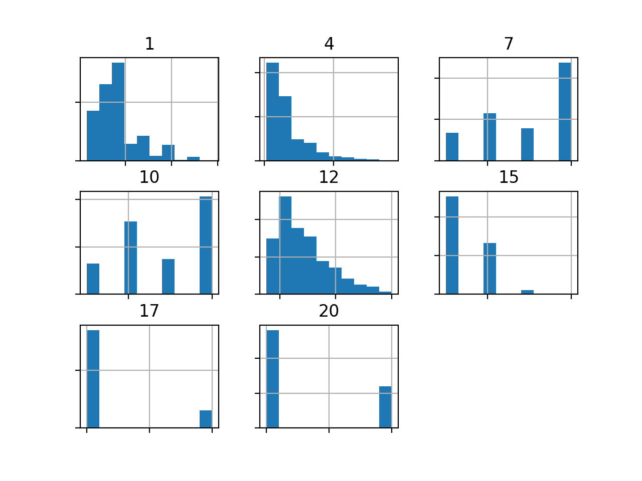
We can also take a look at the distribution of the seven numerical input variables by creating a histogram for each.
First, we can select the columns with numeric variables by calling the select_dtypes() function on the DataFrame. We can then select just those columns from the DataFrame. We would expect there to be seven, plus the numerical class labels.
# select a subset of the dataframe with the chosen columns
subset=df[num_ix]
# create a histogram plot of each numeric variable
ax=subset.hist()
# disable axis labels to avoid the clutter
foraxis inax.flatten():
axis.set_xticklabels([])
axis.set_yticklabels([])
# show the plot
pyplot.show()
Running the example creates the figure with one histogram subplot for each of the seven input variables and one class label in the dataset. The title of each subplot indicates the column number in the DataFrame (e.g. zero-offset from 0 to 20).
We can see many different distributions, some with Gaussian-like distributions, others with seemingly exponential or discrete distributions.
Depending on the choice of modeling algorithms, we would expect scaling the distributions to the same range to be useful, and perhaps the use of some power transforms.
Histogram of Numeric Variables in the German Credit Dataset
Now that we have reviewed the dataset, let’s look at developing a test harness for evaluating candidate models.
Model Test and Baseline Result
We will evaluate candidate models using repeated stratified k-fold cross-validation.
The k-fold cross-validation procedure provides a good general estimate of model performance that is not too optimistically biased, at least compared to a single train-test split. We will use k=10, meaning each fold will contain about 1000/10 or 100 examples.
Stratified means that each fold will contain the same mixture of examples by class, that is about 70 percent to 30 percent good to bad customers. Repeated means that the evaluation process will be performed multiple times to help avoid fluke results and better capture the variance of the chosen model. We will use three repeats.
This means a single model will be fit and evaluated 10 * 3 or 30 times and the mean and standard deviation of these runs will be reported.
We will predict class labels of whether a customer is good or not. Therefore, we need a measure that is appropriate for evaluating the predicted class labels.
The focus of the task is on the positive class (bad customers). Precision and recall are a good place to start. Maximizing precision will minimize the false positives and maximizing recall will minimize the false negatives in the predictions made by a model.
Using the F-Measure will calculate the harmonic mean between precision and recall. This is a good single number that can be used to compare and select a model on this problem. The issue is that false negatives are more damaging than false positives.
Remember that false negatives on this dataset are cases of a bad customer being marked as a good customer and being given a loan. False positives are cases of a good customer being marked as a bad customer and not being given a loan.
False Negative: Bad Customer (class 1) predicted as a Good Customer (class 0).
False Positive: Good Customer (class 0) predicted as a Bad Customer (class 1).
False negatives are more costly to the bank than false positives.
Cost(False Negatives) > Cost(False Positives)
Put another way, we are interested in the F-measure that will summarize a model’s ability to minimize misclassification errors for the positive class, but we want to favor models that are better are minimizing false negatives over false positives.
This can be achieved by using a version of the F-measure that calculates a weighted harmonic mean of precision and recall but favors higher recall scores over precision scores. This is called the Fbeta-measure, a generalization of F-measure, where “beta” is a parameter that defines the weighting of the two scores.
We will use this measure to evaluate models on the German credit dataset. This can be achieved using the fbeta_score() scikit-learn function.
We can define a function to load the dataset and split the columns into input and output variables. We will one-hot encode the categorical variables and label encode the target variable. You might recall that a one-hot encoding replaces the categorical variable with one new column for each value of the variable and marks values with a 1 in the column for that value.
First, we must split the DataFrame into input and output variables.
Next, we need to select all input variables that are categorical, then apply a one-hot encoding and leave the numerical variables untouched.
This can be achieved using a ColumnTransformer and defining the transform as a OneHotEncoder applied only to the column indices for categorical variables.
Finally, we can evaluate a baseline model on the dataset using this test harness.
A model that predicts the minority class for examples will achieve a maximum recall score and a baseline precision score. This provides a baseline in model performance on this problem by which all other models can be compared.
This can be achieved using the DummyClassifier class from the scikit-learn library and setting the “strategy” argument to “constant” and the “constant” argument to “1” for the minority class.
Tying this together, the complete example of loading the German Credit dataset, evaluating a baseline model, and reporting the performance is listed below.
1
2
3
4
5
6
7
8
9
10
11
12
13
14
15
16
17
18
19
20
21
22
23
24
25
26
27
28
29
30
31
32
33
34
35
36
37
38
39
40
41
42
43
44
45
46
47
48
49
50
51
52
53
54
55
56
# test harness and baseline model evaluation for the german credit dataset
from collections import Counter
from numpy import mean
from numpy import std
from pandas import read_csv
from sklearn.preprocessing import LabelEncoder
from sklearn.preprocessing import OneHotEncoder
from sklearn.compose import ColumnTransformer
from sklearn.model_selection import cross_val_score
from sklearn.model_selection import RepeatedStratifiedKFold
Running the example first loads and summarizes the dataset.
We can see that we have the correct number of rows loaded, and through the one-hot encoding of the categorical input variables, we have increased the number of input variables from 20 to 61. That suggests that the 13 categorical variables were encoded into a total of 54 columns.
Importantly, we can see that the class labels have the correct mapping to integers with 0 for the majority class and 1 for the minority class, customary for imbalanced binary classification dataset.
Next, the average of the F2-Measure scores is reported.
In this case, we can see that the baseline algorithm achieves an F2-Measure of about 0.682. This score provides a lower limit on model skill; any model that achieves an average F2-Measure above about 0.682 has skill, whereas models that achieve a score below this value do not have skill on this dataset.
1
2
(1000, 61) (1000,) Counter({0: 700, 1: 300})
Mean F2: 0.682 (0.000)
Now that we have a test harness and a baseline in performance, we can begin to evaluate some models on this dataset.
Evaluate Models
In this section, we will evaluate a suite of different techniques on the dataset using the test harness developed in the previous section.
The goal is to both demonstrate how to work through the problem systematically and to demonstrate the capability of some techniques designed for imbalanced classification problems.
The reported performance is good, but not highly optimized (e.g. hyperparameters are not tuned).
Can you do better? If you can achieve better F2-Measure performance using the same test harness, I’d love to hear about it. Let me know in the comments below.
Evaluate Machine Learning Algorithms
Let’s start by evaluating a mixture of probabilistic machine learning models on the dataset.
It can be a good idea to spot check a suite of different linear and nonlinear algorithms on a dataset to quickly flush out what works well and deserves further attention, and what doesn’t.
We will evaluate the following machine learning models on the German credit dataset:
Logistic Regression (LR)
Linear Discriminant Analysis (LDA)
Naive Bayes (NB)
Gaussian Process Classifier (GPC)
Support Vector Machine (SVM)
We will use mostly default model hyperparameters.
We will define each model in turn and add them to a list so that we can evaluate them sequentially. The get_models() function below defines the list of models for evaluation, as well as a list of model short names for plotting the results later.
We can then enumerate the list of models in turn and evaluate each, storing the scores for later evaluation.
We will one-hot encode the categorical input variables as we did in the previous section, and in this case, we will normalize the numerical input variables. This is best performed using the MinMaxScaler within each fold of the cross-validation evaluation process.
An easy way to implement this is to use a Pipeline where the first step is a ColumnTransformer that applies a OneHotEncoder to just the categorical variables, and a MinMaxScaler to just the numerical input variables. To achieve this, we need a list of the column indices for categorical and numerical input variables.
We can update the load_dataset() to return the column indexes as well as the input and output elements of the dataset. The updated version of this function is listed below.
# label encode the target variable to have the classes 0 and 1
y=LabelEncoder().fit_transform(y)
returnX.values,y,cat_ix,num_ix
We can then call this function to get the data and the list of categorical and numerical variables.
1
2
3
4
5
...
# define the location of the dataset
full_path='german.csv'
# load the dataset
X,y,cat_ix,num_ix=load_dataset(full_path)
This can be used to prepare a Pipeline to wrap each model prior to evaluating it.
First, the ColumnTransformer is defined, which specifies what transform to apply to each type of column, then this is used as the first step in a Pipeline that ends with the specific model that will be fit and evaluated.
Running the example evaluates each algorithm in turn and reports the mean and standard deviation F2-Measure.
Note: Your results may vary given the stochastic nature of the algorithm or evaluation procedure, or differences in numerical precision. Consider running the example a few times and compare the average outcome.
In this case, we can see that none of the tested models have an F2-measure above the default of predicting the majority class in all cases (0.682). None of the models are skillful. This is surprising, although suggests that perhaps the decision boundary between the two classes is noisy.
1
2
3
4
5
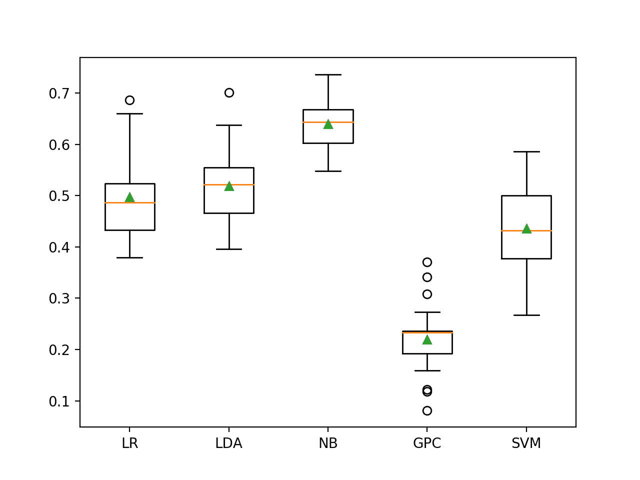
>LR 0.497 (0.072)
>LDA 0.519 (0.072)
>NB 0.639 (0.049)
>GPC 0.219 (0.061)
>SVM 0.436 (0.077)
A figure is created showing one box and whisker plot for each algorithm’s sample of results. The box shows the middle 50 percent of the data, the orange line in the middle of each box shows the median of the sample, and the green triangle in each box shows the mean of the sample.
Box and Whisker Plot of Machine Learning Models on the Imbalanced German Credit Dataset
Now that we have some results, let’s see if we can improve them with some undersampling.
Evaluate Undersampling
Undersampling is perhaps the least widely used technique when addressing an imbalanced classification task as most of the focus is put on oversampling the majority class with SMOTE.
Undersampling can help to remove examples from the majority class along the decision boundary that make the problem challenging for classification algorithms.
In this experiment we will test the following undersampling algorithms:
Tomek Links (TL)
Edited Nearest Neighbors (ENN)
Repeated Edited Nearest Neighbors (RENN)
One Sided Selection (OSS)
Neighborhood Cleaning Rule (NCR)
The Tomek Links and ENN methods select examples from the majority class to delete, whereas OSS and NCR both select examples to keep and examples to delete. We will use the balanced version of the logistic regression algorithm to test each undersampling method, to keep things simple.
The get_models() function from the previous section can be updated to return a list of undersampling techniques to test with the logistic regression algorithm. We use the implementations of these algorithms from the imbalanced-learn library.
The updated version of the get_models() function defining the undersampling methods is listed below.
1
2
3
4
5
6
7
8
9
10
11
12
13
14
15
16
17
18
19
# define undersampling models to test
def get_models():
models,names=list(),list()
# TL
models.append(TomekLinks())
names.append('TL')
# ENN
models.append(EditedNearestNeighbours())
names.append('ENN')
# RENN
models.append(RepeatedEditedNearestNeighbours())
names.append('RENN')
# OSS
models.append(OneSidedSelection())
names.append('OSS')
# NCR
models.append(NeighbourhoodCleaningRule())
names.append('NCR')
returnmodels,names
The Pipeline provided by scikit-learn does not know about undersampling algorithms. Therefore, we must use the Pipeline implementation provided by the imbalanced-learn library.
As in the previous section, the first step of the pipeline will be one hot encoding of categorical variables and normalization of numerical variables, and the final step will be fitting the model. Here, the middle step will be the undersampling technique, correctly applied within the cross-validation evaluation on the training dataset only.
Tying this together, the complete example of evaluating logistic regression with different undersampling methods on the German credit dataset is listed below.
We would expect the undersampling to to result in a lift on skill in logistic regression, ideally above the baseline performance of predicting the minority class in all cases.
The complete example is listed below.
1
2
3
4
5
6
7
8
9
10
11
12
13
14
15
16
17
18
19
20
21
22
23
24
25
26
27
28
29
30
31
32
33
34
35
36
37
38
39
40
41
42
43
44
45
46
47
48
49
50
51
52
53
54
55
56
57
58
59
60
61
62
63
64
65
66
67
68
69
70
71
72
73
74
75
76
77
78
79
80
81
82
83
84
85
86
87
88
89
90
91
92
# evaluate undersampling with logistic regression on the imbalanced german credit dataset
from numpy import mean
from numpy import std
from pandas import read_csv
from sklearn.preprocessing import LabelEncoder
from sklearn.preprocessing import OneHotEncoder
from sklearn.preprocessing import MinMaxScaler
from sklearn.compose import ColumnTransformer
from sklearn.model_selection import cross_val_score
from sklearn.model_selection import RepeatedStratifiedKFold
from sklearn.metrics import fbeta_score
from sklearn.metrics import make_scorer
from matplotlib import pyplot
from sklearn.linear_model import LogisticRegression
from imblearn.pipeline import Pipeline
from imblearn.under_sampling import TomekLinks
from imblearn.under_sampling import EditedNearestNeighbours
from imblearn.under_sampling import RepeatedEditedNearestNeighbours
from imblearn.under_sampling import NeighbourhoodCleaningRule
from imblearn.under_sampling import OneSidedSelection
Running the example evaluates the logistic regression algorithm with five different undersampling techniques.
Note: Your results may vary given the stochastic nature of the algorithm or evaluation procedure, or differences in numerical precision. Consider running the example a few times and compare the average outcome.
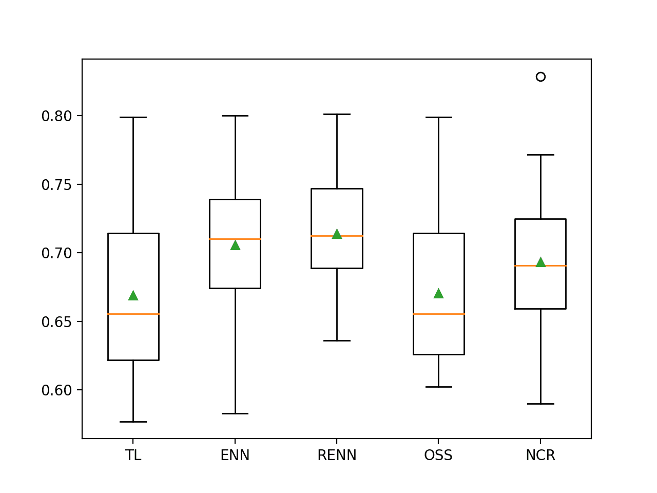
In this case, we can see that three of the five undersampling techniques resulted in an F2-measure that provides an improvement over the baseline of 0.682. Specifically, ENN, RENN and NCR, with repeated edited nearest neighbors resulting in the best performance with an F2-measure of about 0.716.
The results suggest SMOTE achieved the best score with an F2-Measure of 0.604.
1
2
3
4
5
>TL 0.669 (0.057)
>ENN 0.706 (0.048)
>RENN 0.714 (0.041)
>OSS 0.670 (0.054)
>NCR 0.693 (0.052)
Box and whisker plots are created for each evaluated undersampling technique, showing that they generally have the same spread.
It is encouraging to see that for the well performing methods, the boxes spread up around 0.8, and the mean and median for all three methods are are around 0.7. This highlights that the distributions are skewing high and are let down on occasion by a few bad evaluations.
Box and Whisker Plot of Logistic Regression With Undersampling on the Imbalanced German Credit Dataset
Next, let’s see how we might use a final model to make predictions on new data.
Further Model Improvements
This is a new section that provides a minor departure to the above section. Here, we will test specific models that result in a further lift in F2-measure performance and I will update this section as new models are reported/discovered.
Improvement #1: InstanceHardnessThreshold
An F2-measure of about 0.727 can be achieved using balanced Logistic Regression with InstanceHardnessThreshold undersampling.
The complete example is listed below.
1
2
3
4
5
6
7
8
9
10
11
12
13
14
15
16
17
18
19
20
21
22
23
24
25
26
27
28
29
30
31
32
33
34
35
36
37
38
39
40
41
42
43
44
45
46
47
48
49
50
51
52
53
54
55
56
57
58
59
# improve performance on the imbalanced german credit dataset
from numpy import mean
from numpy import std
from pandas import read_csv
from sklearn.preprocessing import LabelEncoder
from sklearn.preprocessing import OneHotEncoder
from sklearn.preprocessing import MinMaxScaler
from sklearn.compose import ColumnTransformer
from sklearn.model_selection import cross_val_score
from sklearn.model_selection import RepeatedStratifiedKFold
from sklearn.metrics import fbeta_score
from sklearn.metrics import make_scorer
from sklearn.linear_model import LogisticRegression
from imblearn.pipeline import Pipeline
from imblearn.under_sampling import InstanceHardnessThreshold
Note: Your results may vary given the stochastic nature of the algorithm or evaluation procedure, or differences in numerical precision. Consider running the example a few times and compare the average outcome.
Running the example gives the follow results.
1
0.727 (0.033)
Improvement #2: SMOTEENN
An F2-measure of about 0.730 can be achieved using LDA with SMOTEENN, where the ENN parameter is set to an ENN instance with sampling_strategy set to majority.
The complete example is listed below.
1
2
3
4
5
6
7
8
9
10
11
12
13
14
15
16
17
18
19
20
21
22
23
24
25
26
27
28
29
30
31
32
33
34
35
36
37
38
39
40
41
42
43
44
45
46
47
48
49
50
51
52
53
54
55
56
57
58
59
60
# improve performance on the imbalanced german credit dataset
from numpy import mean
from numpy import std
from pandas import read_csv
from sklearn.preprocessing import LabelEncoder
from sklearn.preprocessing import OneHotEncoder
from sklearn.preprocessing import MinMaxScaler
from sklearn.compose import ColumnTransformer
from sklearn.model_selection import cross_val_score
from sklearn.model_selection import RepeatedStratifiedKFold
from sklearn.metrics import fbeta_score
from sklearn.metrics import make_scorer
from sklearn.discriminant_analysis import LinearDiscriminantAnalysis
from imblearn.pipeline import Pipeline
from imblearn.combine import SMOTEENN
from imblearn.under_sampling import EditedNearestNeighbours
Note: Your results may vary given the stochastic nature of the algorithm or evaluation procedure, or differences in numerical precision. Consider running the example a few times and compare the average outcome.
Running the example gives the follow results.
1
0.730 (0.046)
Improvement #3: SMOTEENN with StandardScaler and RidgeClassifier
An F2-measure of about 0.741 can be achieved with further improvements to the SMOTEENN using a RidgeClassifier instead of LDA and using a StandardScaler for the numeric inputs instead of a MinMaxScaler.
The complete example is listed below.
1
2
3
4
5
6
7
8
9
10
11
12
13
14
15
16
17
18
19
20
21
22
23
24
25
26
27
28
29
30
31
32
33
34
35
36
37
38
39
40
41
42
43
44
45
46
47
48
49
50
51
52
53
54
55
56
57
58
59
60
# improve performance on the imbalanced german credit dataset
from numpy import mean
from numpy import std
from pandas import read_csv
from sklearn.preprocessing import LabelEncoder
from sklearn.preprocessing import OneHotEncoder
from sklearn.preprocessing import StandardScaler
from sklearn.compose import ColumnTransformer
from sklearn.model_selection import cross_val_score
from sklearn.model_selection import RepeatedStratifiedKFold
from sklearn.metrics import fbeta_score
from sklearn.metrics import make_scorer
from sklearn.linear_model import RidgeClassifier
from imblearn.pipeline import Pipeline
from imblearn.combine import SMOTEENN
from imblearn.under_sampling import EditedNearestNeighbours
Note: Your results may vary given the stochastic nature of the algorithm or evaluation procedure, or differences in numerical precision. Consider running the example a few times and compare the average outcome.
Running the example gives the follow results.
1
0.741 (0.034)
Can you do even better?
Let me know in the comments below.
Make Prediction on New Data
Given the variance in results, a selection of any of the undersampling methods is probably sufficient. In this case, we will select logistic regression with Repeated ENN.
This model had an F2-measure of about about 0.716 on our test harness.
We will use this as our final model and use it to make predictions on new data.
Once defined, we can fit it on the entire training dataset.
1
2
3
...
# fit the model
pipeline.fit(X,y)
Once fit, we can use it to make predictions for new data by calling the predict() function. This will return the class label of 0 for “good customer”, or 1 for “bad customer”.
Importantly, we must use the ColumnTransformer that was fit on the training dataset in the Pipeline to correctly prepare new data using the same transforms.
For example:
1
2
3
4
5
...
# define a row of data
row=[...]
# make prediction
yhat=pipeline.predict([row])
To demonstrate this, we can use the fit model to make some predictions of labels for a few cases where we know if the case is a good customer or bad.
The complete example is listed below.
1
2
3
4
5
6
7
8
9
10
11
12
13
14
15
16
17
18
19
20
21
22
23
24
25
26
27
28
29
30
31
32
33
34
35
36
37
38
39
40
41
42
43
44
45
46
47
48
49
50
51
52
53
54
55
56
57
58
59
60
# fit a model and make predictions for the german credit dataset
from pandas import read_csv
from sklearn.preprocessing import LabelEncoder
from sklearn.preprocessing import OneHotEncoder
from sklearn.preprocessing import MinMaxScaler
from sklearn.compose import ColumnTransformer
from sklearn.linear_model import LogisticRegression
from imblearn.pipeline import Pipeline
from imblearn.under_sampling import RepeatedEditedNearestNeighbours
Running the example first fits the model on the entire training dataset.
Then the fit model used to predict the label of a good customer for cases chosen from the dataset file. We can see that most cases are correctly predicted. This highlights that although we chose a good model, it is not perfect.
Then some cases of actual bad customers are used as input to the model and the label is predicted. As we might have hoped, the correct labels are predicted for all cases.
1
2
3
4
5
6
7
8
Good Customers:
>Predicted=0 (expected 0)
>Predicted=0 (expected 0)
>Predicted=0 (expected 0)
Bad Customers:
>Predicted=0 (expected 1)
>Predicted=1 (expected 1)
>Predicted=1 (expected 1)
Further Reading
This section provides more resources on the topic if you are looking to go deeper.
It provides self-study tutorials and end-to-end projects on: Performance Metrics, Undersampling Methods, SMOTE, Threshold Moving, Probability Calibration, Cost-Sensitive Algorithms
and much more...
Bring Imbalanced Classification Methods to Your Machine Learning Projects
Employing a 60/40 train-test approach, fitting the various model/sampling combinations to the training data set, and then predicting on the test data set, the best f2 scores appear to be 0.738 for RC RENN (min-max normalization) and 0.737 for LDA RENN (min-max normalization). Using RC SMOTEENN returns f2 scores of 0.732 (min-max normalization) and 0.707 (mean standardization). Of course, these score will vary as a result of the randomness in the split. After having employed cross-val to identify promising models, I like to then apply them in train-test to produce confusion matrices. Confusion matrix heat maps help visualization of the trade-off between overall accuracy (in his case, generally in the 0.6 to 0.7 range) and the reduction in false negatives (and shifting of misclassification errors to false positives) in optimizing based on he the f2 measure. For example, in the case of RC SMOTEENN (min-max normalization), out of the 400 samples in the test set, 252 were classified correctly (overall accuracy = 0.63), but of the 148 misclassified samples, only 13 were false negatives and 135 were false positives.
I understood that SMOTE techniques (for minority oversampling improvement) are not applicable to images data. because only apply to tabular data and also we have a similar techniques such as data-augmentation for image data…OK
But what about Undersampling techniques such as (TL, ENN, RENN, OSS, NCR) , they can not be also used for image data ? and is there any similar counterpart for image data such as the opposite of data-augmentation?
Most methods are based on kNN which would be a mess on pixel data. Maybe people are exploring similarity metrics in this context, I have no idea.
You can achieve similar rebalancing effects with a carefully crafted data augmentation implementation – controlling the balance of samples yielded in each batch. This is where I would focus.
from imblearn.combine import SMOTEENN
# define the data sampling
sampling = SMOTEENN(enn=EditedNearestNeighbours(sampling_strategy=’majority’, random_state=42))
When I transform the data step by step i.e first transformed data using column transformer and then resampled using SMOTEEN.
Score of dummy model :-
Mean F2:- 0.58 , standard deviation:- 0.000
Usually, I got this score, when I had not resampled the training data. I am confused, why combining all pipelines & column transformer are not giving the same results. Can you please help me in this?
Hi Jason,
Thank you for the notebook.
I combine a cost-sensitive algorithm with a under sampling technique, then use a heuristic to improve the score. Specifically i use ridge classifier with weights and Edited Nearest Neighbors, the number of neighbors also was a parameter in the heuristic. The best result was 0.7503 in the F2-measure.
Thanks a lot for sharing your knowledge. I found the tutorial quite enlightening, and I was able to get clarity on many issues I had on binary classification using imbalanced training datasets.
To try and improve on your result and to achieve a better F2-Measure, I first used the CalibratedClassifierCV class to wrap the models. I set the method parameter to ‘isotonic’ and class_weight to ‘balanced’ for SVM and LR. From this, I obtained the following values:
Clearly an inferior outcome for SVM as well as the first 3.
I managed to record the most profound improvement in the skill of my balanced calibrated SVM using undersampling. The results of the evaluation of the SVM algorithm with five different undersampling techniques were as follows.
RENN and ENN achieved a massive improvement of the SVM over the baseline of 0.682. I found this remarkable given that without the probability calibration and undersampling of the SVM, the result was 0.436 (completely no skill) for the SVM.
I am working on a binary classification project (credit scoring) using users’ mobile phone metadata. Any tips on what to watch out for or consider?
Thanks a lot for the tutorial, it is very helpful. I want to ask only one thing. Why don’t we use “DummyClassifier” model with undersampling methods and take the corresponding f2-score as a base model to outperform? If we undersample and use “DummyClassifier” model, we should get a F-2 score of around 0.83. So, no skill model (predicting everything 1) should have a lot higher f-score.
Why do we need the “evaluate_model” function, specifically cross_val_score inside? Can’t we just use fbeta_score(y_true, y_pred, beta=2) and calculate f2 score directly? Thanks.
I need to write the code that fulfills these 3 points:
1) Develop a prediction model to classify the customers as good or bad;
2) Cluster the customers into various groups;
3) Provide some ideas on how frequent pattern mining could be utilized to uncover some patterns in the data and/or to enhance the classification;
I am fairly new to this machine learning journey and your articles are great at explaining complex topic simplistically. Thanks again.
With regards to this problem, I have managed to get a score of between 91-92% on train and test data, with below Logistic Regression parameters. This is without any undersampling. Below is the approach. It will be great if you could spot anything I am doing wrong, as I am suspicious of such high results.
Thanks for the tutorial. Great job! I have 2 questions:
1. I didn’t observe any feature selection in your model. Did you use any that I couldn’t realize? If not, do you think selecting features could improve the model?
2. I’m developing an imbalanced classification model w/ only 300 rows dataset. In this case, is it better to use oversampling rather than undersampling due to the low amount of data?
I see that you have one hot encoded the categorical data, applied a scaler on the numerical data and then applied a synthetic technique like SMOTE() to over sample the data.
What kind of data points are generated on the one hot encoded fields? Will they still be of binary nature or will there be synthetic points created within the encoded features?
If it is the latter, would that make sense for a model to learn given that it would never truly see a synthetic point or a float data type for a field that could only ever be binary.


Very Nice Tutorial with code.
Thanks!
fantastic notebook
Thanks.
Jason:
Employing a 60/40 train-test approach, fitting the various model/sampling combinations to the training data set, and then predicting on the test data set, the best f2 scores appear to be 0.738 for RC RENN (min-max normalization) and 0.737 for LDA RENN (min-max normalization). Using RC SMOTEENN returns f2 scores of 0.732 (min-max normalization) and 0.707 (mean standardization). Of course, these score will vary as a result of the randomness in the split. After having employed cross-val to identify promising models, I like to then apply them in train-test to produce confusion matrices. Confusion matrix heat maps help visualization of the trade-off between overall accuracy (in his case, generally in the 0.6 to 0.7 range) and the reduction in false negatives (and shifting of misclassification errors to false positives) in optimizing based on he the f2 measure. For example, in the case of RC SMOTEENN (min-max normalization), out of the 400 samples in the test set, 252 were classified correctly (overall accuracy = 0.63), but of the 148 misclassified samples, only 13 were false negatives and 135 were false positives.
Nice work Ron!
Fantastic work Jason…
Thanks!
Hi Jason,
Thank your for your tutorial!
I understood that SMOTE techniques (for minority oversampling improvement) are not applicable to images data. because only apply to tabular data and also we have a similar techniques such as data-augmentation for image data…OK
But what about Undersampling techniques such as (TL, ENN, RENN, OSS, NCR) , they can not be also used for image data ? and is there any similar counterpart for image data such as the opposite of data-augmentation?
regards
Most methods are based on kNN which would be a mess on pixel data. Maybe people are exploring similarity metrics in this context, I have no idea.
You can achieve similar rebalancing effects with a carefully crafted data augmentation implementation – controlling the balance of samples yielded in each batch. This is where I would focus.
Hi Jason,
Thanks for wonderful, articles. These helps me a lot. I have a query.
I had defined below instructions:
num_pipeline = make_pipeline(SimpleImputer(strategy=’median’), MinMaxScaler())
cat_pipeline = make_pipeline(OneHotEncoder())
column_transformer = make_column_transformer((num_pipeline, num_cols),
(cat_pipeline, cat_cols))
from imblearn.combine import SMOTEENN
# define the data sampling
sampling = SMOTEENN(enn=EditedNearestNeighbours(sampling_strategy=’majority’, random_state=42))
When I transform the data step by step i.e first transformed data using column transformer and then resampled using SMOTEEN.
c_train_feature_df = column_transformer.fit_transform(train_feature_df)
# Resampled data in the below line
s_train_feature_df, s_train_target_df= sampling.fit_resample(c_train_feature_df, train_target_df)
In this case score of dummy model is (‘dummy = DummyClassifier(strategy=’constant’, constant=1)’)
Score of dummy model :-
Mean F2:- 0.876 , standard deviation:- 0.000
Now, when I used all above pipelines & column transformer inside a new pipeline like below,
model_pipeline = Pipeline(steps=[(‘ct’, column_transformer), \
(‘s’, sampling), (‘m’, dummy)])
I got below score of dummy model.
Score of dummy model :-
Mean F2:- 0.58 , standard deviation:- 0.000
Usually, I got this score, when I had not resampled the training data. I am confused, why combining all pipelines & column transformer are not giving the same results. Can you please help me in this?
Nice work, sorry I cannot debug your code example:
https://machinelearningmastery.com/faq/single-faq/can-you-read-review-or-debug-my-code
Hi Jason,
Thank you for the notebook.
I combine a cost-sensitive algorithm with a under sampling technique, then use a heuristic to improve the score. Specifically i use ridge classifier with weights and Edited Nearest Neighbors, the number of neighbors also was a parameter in the heuristic. The best result was 0.7503 in the F2-measure.
Well done!
Hi Jason
Thanks a lot for sharing your knowledge. I found the tutorial quite enlightening, and I was able to get clarity on many issues I had on binary classification using imbalanced training datasets.
To try and improve on your result and to achieve a better F2-Measure, I first used the CalibratedClassifierCV class to wrap the models. I set the method parameter to ‘isotonic’ and class_weight to ‘balanced’ for SVM and LR. From this, I obtained the following values:
>LR 0.460 (0.069)
>LDA 0.476 (0.083)
>NB 0.374 (0.087)
>GPC 0.354 (0.063)
>SVM 0.485 (0.072
The only marginal improvement I noticed was for SVM and GPC. LR, LDA, and NB values were poor.
I retained ‘isotonic’ as method and dropped class_weight argument for SVM and LR the results were as follows
>LR 0.463 (0.072)
>LDA 0.476 (0.083)
>NB 0.374 (0.087)
>GPC 0.354 (0.063)
>SVM 0.442 (0.081)
Clearly an inferior outcome for SVM as well as the first 3.
I managed to record the most profound improvement in the skill of my balanced calibrated SVM using undersampling. The results of the evaluation of the SVM algorithm with five different undersampling techniques were as follows.
>TL 0.516 (0.079)
>ENN 0.683 (0.044)
>RENN 0.714 (0.035)
>OSS 0.517 (0.078)
>NCR 0.674 (0.062)
RENN and ENN achieved a massive improvement of the SVM over the baseline of 0.682. I found this remarkable given that without the probability calibration and undersampling of the SVM, the result was 0.436 (completely no skill) for the SVM.
I am working on a binary classification project (credit scoring) using users’ mobile phone metadata. Any tips on what to watch out for or consider?
Once more thanks a lot for sharing.
Gideon Aswani
Nice work!
Notice we achieved an F2 of up to 0.741 (0.034) in the tutorial.
This framework will help ensure you try a suite of different techniques and get the best from your dataset:
https://machinelearningmastery.com/framework-for-imbalanced-classification-projects/
Hi Jason
Thanks again. Yes, I noticed in the tutorial you achieved 0.741(0.034). That was great. I will use the framework to improve on my work
Thanks a lot for the tutorial, it is very helpful. I want to ask only one thing. Why don’t we use “DummyClassifier” model with undersampling methods and take the corresponding f2-score as a base model to outperform? If we undersample and use “DummyClassifier” model, we should get a F-2 score of around 0.83. So, no skill model (predicting everything 1) should have a lot higher f-score.
We use the dummy classifier to establish a baseline. Any model that does better than it has “skill” on the problem.
It is important that the dummy classifier is as simple as possible.
Hi,
Why do we need the “evaluate_model” function, specifically cross_val_score inside? Can’t we just use fbeta_score(y_true, y_pred, beta=2) and calculate f2 score directly? Thanks.
Ulas
You can calculate the score directly if you make predictions on a hold out dataset.
I need to write the code that fulfills these 3 points:
1) Develop a prediction model to classify the customers as good or bad;
2) Cluster the customers into various groups;
3) Provide some ideas on how frequent pattern mining could be utilized to uncover some patterns in the data and/or to enhance the classification;
a help would be appreciated.
Perhaps this process will help:
https://machinelearningmastery.com/start-here/#process
Hi Jason,
Thanks a lot for this article.
I am fairly new to this machine learning journey and your articles are great at explaining complex topic simplistically. Thanks again.
With regards to this problem, I have managed to get a score of between 91-92% on train and test data, with below Logistic Regression parameters. This is without any undersampling. Below is the approach. It will be great if you could spot anything I am doing wrong, as I am suspicious of such high results.
The only difference is that in preprocessing, I removed all quotes around categorical features, that is present in the dataset.
Thanks again.
Well done!
That is a high score, let me schedule some time to check.
I could not reproduce your result with that model, the best I could get was:
I believe you accidentally reported accuracy instead of F2-Measure via a call to grid.score(). Perhaps that is the cause of your “91-92%” result
You can see my complete code for the grid search listed below
Hi Jason,
Thanks for the tutorial. Great job! I have 2 questions:
1. I didn’t observe any feature selection in your model. Did you use any that I couldn’t realize? If not, do you think selecting features could improve the model?
2. I’m developing an imbalanced classification model w/ only 300 rows dataset. In this case, is it better to use oversampling rather than undersampling due to the low amount of data?
Thanks in advance!
Hi Igor…Feature selection would definitely be an improvement you could implement in this case. Also, the following may be of interest to you:
https://www.kaggle.com/code/rafjaa/dealing-with-very-small-datasets/notebook
Hi James,
The notebook you shared will be really useful. Thanks!
Hi Jason,
I see that you have one hot encoded the categorical data, applied a scaler on the numerical data and then applied a synthetic technique like SMOTE() to over sample the data.
What kind of data points are generated on the one hot encoded fields? Will they still be of binary nature or will there be synthetic points created within the encoded features?
If it is the latter, would that make sense for a model to learn given that it would never truly see a synthetic point or a float data type for a field that could only ever be binary.
Hi Vivek…The following resource may be of interest:
https://machinelearningmastery.com/smote-oversampling-for-imbalanced-classification/