Predictive Model for the Phoneme Imbalanced Classification Dataset

Many binary classification tasks do not have an equal number of examples from each class, e.g. the class distribution is skewed or imbalanced.

Nevertheless, accuracy is equally important in both classes.

An example is the classification of vowel sounds from European languages as either nasal or oral on speech recognition where there are many more examples of nasal than oral vowels. Classification accuracy is important for both classes, although accuracy as a metric cannot be used directly. Additionally, data sampling techniques may be required to transform the training dataset to make it more balanced when fitting machine learning algorithms.

In this tutorial, you will discover how to develop and evaluate models for imbalanced binary classification of nasal and oral phonemes.

After completing this tutorial, you will know:

• How to load and explore the dataset and generate ideas for data preparation and model selection.
• How to evaluate a suite of machine learning models and improve their performance with data oversampling techniques.
• How to fit a final model and use it to predict class labels for specific cases.

Kick-start your project with my new book Imbalanced Classification with Python, including step-by-step tutorials and the Python source code files for all examples.

Let’s get started.

• Updated Jan/2021: Updated links for API documentation.

Predictive Model for the Phoneme Imbalanced Classification Dataset
Photo by Ed Dunens, some rights reserved.

Tutorial Overview

This tutorial is divided into five parts; they are:

1. Phoneme Dataset
2. Explore the Dataset
3. Model Test and Baseline Result
4. Evaluate Models
   1. Evaluate Machine Learning Algorithms
   2. Evaluate Data Oversampling Algorithms
5. Make Predictions on New Data

Phoneme Dataset

In this project, we will use a standard imbalanced machine learning dataset referred to as the “Phoneme” dataset.

This dataset is credited to the ESPRIT (European Strategic Program on Research in Information Technology) project titled “ROARS” (Robust Analytical Speech Recognition System) and described in progress reports and technical reports from that project.

The goal of the ROARS project is to increase the robustness of an existing analytical speech recognition system (i,e., one using knowledge about syllables, phonemes and phonetic features), and to use it as part of a speech understanding system with connected words and dialogue capability. This system will be evaluated for a specific application in two European languages

— ESPRIT: The European Strategic Programme for Research and development in Information Technology.

The goal of the dataset was to distinguish between nasal and oral vowels.

Vowel sounds were spoken and recorded to digital files. Then audio features were automatically extracted from each sound.

Five different attributes were chosen to characterize each vowel: they are the amplitudes of the five first harmonics AHi, normalised by the total energy Ene (integrated on all the frequencies): AHi/Ene. Each harmonic is signed: positive when it corresponds to a local maximum of the spectrum and negative otherwise.

— Phoneme Dataset Description.

There are two classes for the two types of sounds; they are:

• Class 0: Nasal Vowels (majority class).
• Class 1: Oral Vowels (minority class).

Next, let’s take a closer look at the data.

Explore the Dataset

The Phoneme dataset is a widely used standard machine learning dataset, used to explore and demonstrate many techniques designed specifically for imbalanced classification.

One example is the popular SMOTE data oversampling technique.

First, download the dataset and save it in your current working directory with the name “phoneme.csv“.

• Download Phoneme Dataset (phoneme.csv)

Review the contents of the file.

The first few lines of the file should look as follows:

We can see that the given input variables are numeric and class labels are 0 and 1 for nasal and oral respectively.

The dataset can be loaded as a DataFrame using the read_csv() Pandas function, specifying the location and the fact that there is no header line.

Once loaded, we can summarize the number of rows and columns by printing the shape of the DataFrame.

We can also summarize the number of examples in each class using the Counter object.

Tying this together, the complete example of loading and summarizing the dataset is listed below.

Running the example first loads the dataset and confirms the number of rows and columns, that is 5,404 rows and five input variables and one target variable.

The class distribution is then summarized, confirming a modest class imbalance with approximately 70 percent for the majority class (nasal) and approximately 30 percent for the minority class (oral).

We can also take a look at the distribution of the five numerical input variables by creating a histogram for each.

The complete example is listed below.

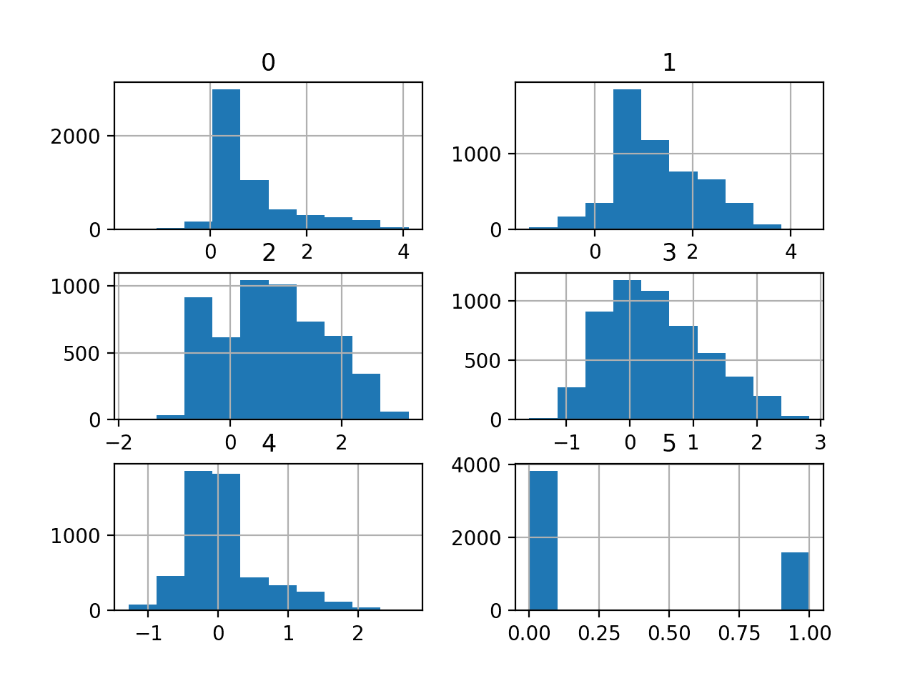
Running the example creates the figure with one histogram subplot for each of the five numerical input variables in the dataset, as well as the numerical class label.

We can see that the variables have differing scales, although most appear to have a Gaussian or Gaussian-like distribution.

Depending on the choice of modeling algorithms, we would expect scaling the distributions to the same range to be useful, and perhaps standardize the use of some power transforms.

Histogram Plots of the Variables for the Phoneme Dataset

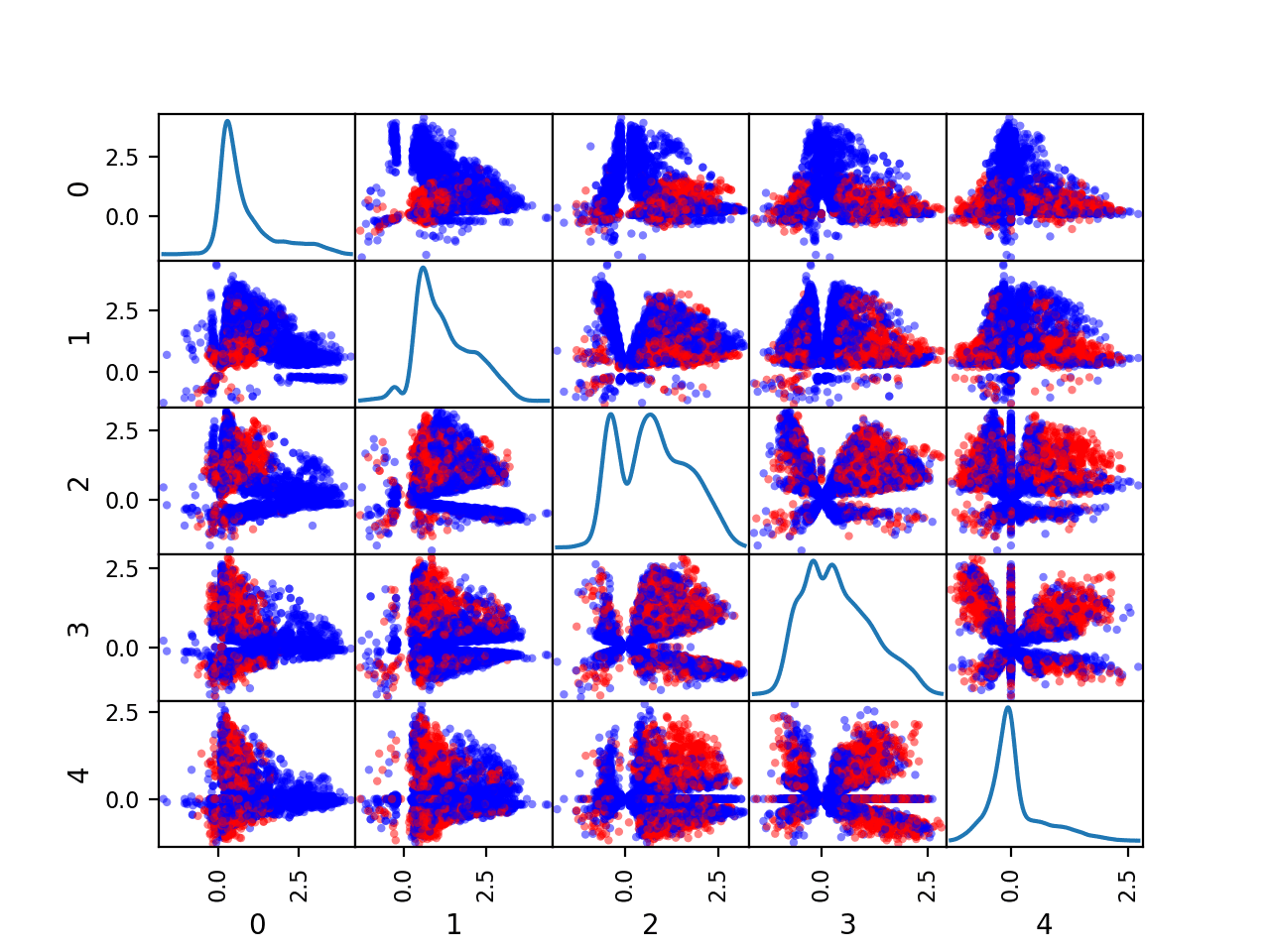
We can also create a scatter plot for each pair of input variables, called a scatter plot matrix.

This can be helpful to see if any variables relate to each other or change in the same direction, e.g. are correlated.

We can also color the dots of each scatter plot according to the class label. In this case, the majority class (nasal) will be mapped to blue dots and the minority class (oral) will be mapped to red dots.

The complete example is listed below.

Running the example creates a figure showing the scatter plot matrix, with five plots by five plots, comparing each of the five numerical input variables with each other. The diagonal of the matrix shows the density distribution of each variable.

Each pairing appears twice, both above and below the top-left to bottom-right diagonal, providing two ways to review the same variable interactions.

We can see that the distributions for many variables do differ for the two class labels, suggesting that some reasonable discrimination between the classes will be feasible.

Scatter Plot Matrix by Class for the Numerical Input Variables in the Phoneme Dataset

Now that we have reviewed the dataset, let’s look at developing a test harness for evaluating candidate models.

Model Test and Baseline Result

We will evaluate candidate models using repeated stratified k-fold cross-validation.

The k-fold cross-validation procedure provides a good general estimate of model performance that is not too optimistically biased, at least compared to a single train-test split. We will use k=10, meaning each fold will contain about 5404/10 or about 540 examples.

Stratified means that each fold will contain the same mixture of examples by class, that is about 70 percent to 30 percent nasal to oral vowels. Repetition indicates that the evaluation process will be performed multiple times to help avoid fluke results and better capture the variance of the chosen model. We will use three repeats.

This means a single model will be fit and evaluated 10 * 3, or 30, times and the mean and standard deviation of these runs will be reported.

This can be achieved using the RepeatedStratifiedKFold scikit-learn class.

Class labels will be predicted and both class labels are equally important. Therefore, we will select a metric that quantifies the performance of a model on both classes separately.

You may remember that the sensitivity is a measure of the accuracy for the positive class and specificity is a measure of the accuracy of the negative class.

• Sensitivity = TruePositives / (TruePositives + FalseNegatives)
• Specificity = TrueNegatives / (TrueNegatives + FalsePositives)

The G-mean seeks a balance of these scores, the geometric mean, where poor performance for one or the other results in a low G-mean score.

• G-Mean = sqrt(Sensitivity * Specificity)

We can calculate the G-mean for a set of predictions made by a model using the geometric_mean_score() function provided by the imbalanced-learn library.

We can define a function to load the dataset and split the columns into input and output variables. The load_dataset() function below implements this.

We can then define a function that will evaluate a given model on the dataset and return a list of G-Mean scores for each fold and repeat. The evaluate_model() function below implements this, taking the dataset and model as arguments and returning the list of scores.

Finally, we can evaluate a baseline model on the dataset using this test harness.

A model that predicts the majority class label (0) or the minority class label (1) for all cases will result in a G-mean of zero. As such, a good default strategy would be to randomly predict one class label or another with a 50 percent probability and aim for a G-mean of about 0.5.

This can be achieved using the DummyClassifier class from the scikit-learn library and setting the “strategy” argument to ‘uniform‘.

Once the model is evaluated, we can report the mean and standard deviation of the G-mean scores directly.

Tying this together, the complete example of loading the dataset, evaluating a baseline model, and reporting the performance is listed below.

Running the example first loads and summarizes the dataset.

We can see that we have the correct number of rows loaded and that we have five audio-derived input variables.

Next, the average of the G-Mean scores is reported.

In this case, we can see that the baseline algorithm achieves a G-Mean of about 0.509, close to the theoretical maximum of 0.5. This score provides a lower limit on model skill; any model that achieves an average G-Mean above about 0.509 (or really above 0.5) has skill, whereas models that achieve a score below this value do not have skill on this dataset.

Now that we have a test harness and a baseline in performance, we can begin to evaluate some models on this dataset.

Evaluate Models

In this section, we will evaluate a suite of different techniques on the dataset using the test harness developed in the previous section.

The goal is to both demonstrate how to work through the problem systematically and to demonstrate the capability of some techniques designed for imbalanced classification problems.

The reported performance is good, but not highly optimized (e.g. hyperparameters are not tuned).

You can do better? If you can achieve better G-mean performance using the same test harness, I’d love to hear about it. Let me know in the comments below.

Evaluate Machine Learning Algorithms

Let’s start by evaluating a mixture of machine learning models on the dataset.

It can be a good idea to spot check a suite of different linear and nonlinear algorithms on a dataset to quickly flush out what works well and deserves further attention, and what doesn’t.

We will evaluate the following machine learning models on the phoneme dataset:

• Logistic Regression (LR)
• Support Vector Machine (SVM)
• Bagged Decision Trees (BAG)
• Random Forest (RF)
• Extra Trees (ET)

We will use mostly default model hyperparameters, with the exception of the number of trees in the ensemble algorithms, which we will set to a reasonable default of 1,000.

We will define each model in turn and add them to a list so that we can evaluate them sequentially. The get_models() function below defines the list of models for evaluation, as well as a list of model short names for plotting the results later.

We can then enumerate the list of models in turn and evaluate each, reporting the mean G-Mean and storing the scores for later plotting.

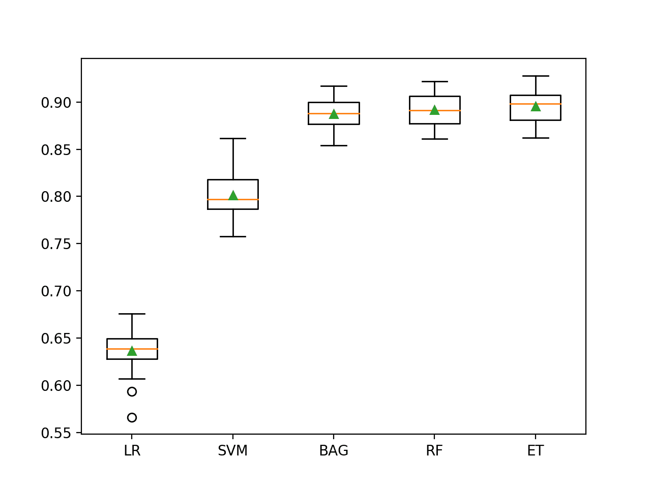
At the end of the run, we can plot each sample of scores as a box and whisker plot with the same scale so that we can directly compare the distributions.

Tying this all together, the complete example of evaluating a suite of machine learning algorithms on the phoneme dataset is listed below.

Running the example evaluates each algorithm in turn and reports the mean and standard deviation G-Mean.

Note: Your results may vary given the stochastic nature of the algorithm or evaluation procedure, or differences in numerical precision. Consider running the example a few times and compare the average outcome.

In this case, we can see that all of the tested algorithms have skill, achieving a G-Mean above the default of 0.5 The results suggest that the ensemble of decision tree algorithms perform better on this dataset with perhaps Extra Trees (ET) performing the best with a G-Mean of about 0.896.

A figure is created showing one box and whisker plot for each algorithm’s sample of results. The box shows the middle 50 percent of the data, the orange line in the middle of each box shows the median of the sample, and the green triangle in each box shows the mean of the sample.

We can see that all three ensembles of trees algorithms (BAG, RF, and ET) have a tight distribution and a mean and median that closely align, perhaps suggesting a non-skewed and Gaussian distribution of scores, e.g. stable.

Box and Whisker Plot of Machine Learning Models on the Imbalanced Phoneme Dataset

Now that we have a good first set of results, let’s see if we can improve them with data oversampling methods.

Evaluate Data Oversampling Algorithms

Data sampling provides a way to better prepare the imbalanced training dataset prior to fitting a model.

The simplest oversampling technique is to duplicate examples in the minority class, called random oversampling. Perhaps the most popular oversampling method is the SMOTE oversampling technique for creating new synthetic examples for the minority class.

We will test five different oversampling methods; specifically:

• Random Oversampling (ROS)
• SMOTE (SMOTE)
• BorderLine SMOTE (BLSMOTE)
• SVM SMOTE (SVMSMOTE)
• ADASYN (ADASYN)

Each technique will be tested with the best performing algorithm from the previous section, specifically Extra Trees.

We will use the default hyperparameters for each oversampling algorithm, which will oversample the minority class to have the same number of examples as the majority class in the training dataset.

The expectation is that each oversampling technique will result in a lift in performance compared to the algorithm without oversampling with the smallest lift provided by Random Oversampling and perhaps the best lift provided by SMOTE or one of its variations.

We can update the get_models() function to return lists of oversampling algorithms to evaluate; for example:

We can then enumerate each and create a Pipeline from the imbalanced-learn library that is aware of how to oversample a training dataset. This will ensure that the training dataset within the cross-validation model evaluation is sampled correctly, without data leakage that could result in an optimistic evaluation of model performance.

First, we will normalize the input variables because most oversampling techniques will make use of a nearest neighbor algorithm and it is important that all variables have the same scale when using this technique. This will be followed by a given oversampling algorithm, then ending with the Extra Trees algorithm that will be fit on the oversampled training dataset.

Tying this together, the complete example of evaluating oversampling algorithms with Extra Trees on the phoneme dataset is listed below.

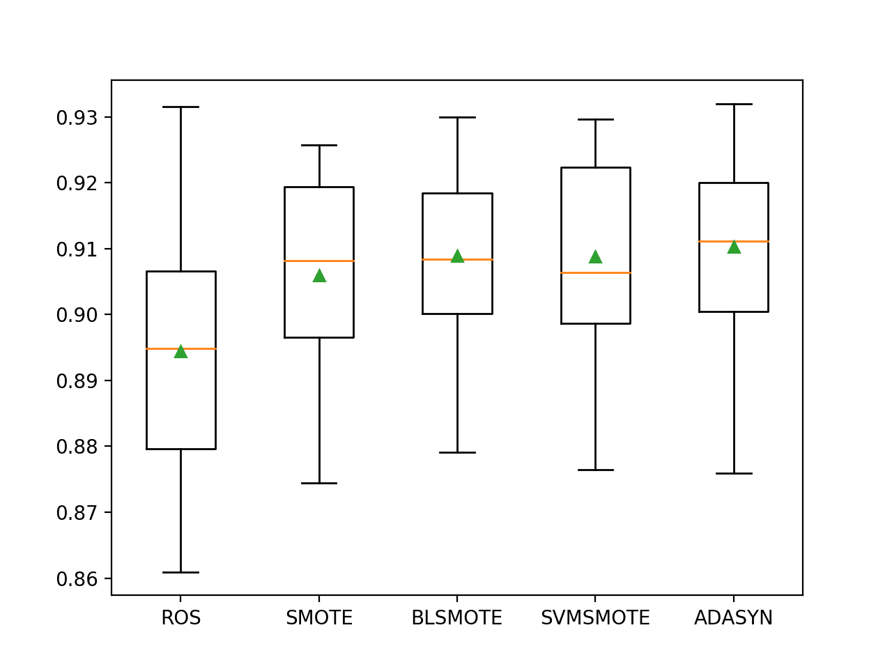
Running the example evaluates each oversampling method with the Extra Trees model on the dataset.

Note: Your results may vary given the stochastic nature of the algorithm or evaluation procedure, or differences in numerical precision. Consider running the example a few times and compare the average outcome.

In this case, as we expected, each oversampling technique resulted in a lift in performance for the ET algorithm without any oversampling (0.896), except the random oversampling technique.

The results suggest that the modified versions of SMOTE and ADASYN performed better than default SMOTE, and in this case, ADASYN achieved the best G-Mean score of 0.910.

The distribution of results can be compared with box and whisker plots.

We can see the distributions all roughly have the same tight distribution and that the difference in means of the results can be used to select a model.

Box and Whisker Plot of Extra Trees Models With Data Oversampling on the Imbalanced Phoneme Dataset

Next, let’s see how we might use a final model to make predictions on new data.

Make Prediction on New Data

In this section, we will fit a final model and use it to make predictions on single rows of data

We will use the ADASYN oversampled version of the Extra Trees model as the final model and a normalization scaling on the data prior to fitting the model and making a prediction. Using the pipeline will ensure that the transform is always performed correctly.

First, we can define the model as a pipeline.

Once defined, we can fit it on the entire training dataset.

Once fit, we can use it to make predictions for new data by calling the predict() function. This will return the class label of 0 for “nasal, or 1 for “oral“.

For example:

To demonstrate this, we can use the fit model to make some predictions of labels for a few cases where we know if the case is nasal or oral.

The complete example is listed below.

Running the example first fits the model on the entire training dataset.

Then the fit model is used to predict the label of nasal cases chosen from the dataset file. We can see that all cases are correctly predicted.

Then some oral cases are used as input to the model and the label is predicted. As we might have hoped, the correct labels are predicted for all cases.

Further Reading

This section provides more resources on the topic if you are looking to go deeper.

Papers

• ESPRIT: The European Strategic Programme for Research and development in Information Technology.

APIs

• sklearn.model_selection.RepeatedStratifiedKFold API.
• sklearn.dummy.DummyClassifier API.
• imblearn.metrics.geometric_mean_score API.

Dataset

• Phoneme Dataset
• Phoneme Dataset Description
• Phoneme Dataset on KEEL
• Phoneme Dataset on the ELENA Project

Summary

In this tutorial, you discovered how to develop and evaluate models for imbalanced binary classification of nasal and oral phonemes.

Specifically, you learned:

• How to load and explore the dataset and generate ideas for data preparation and model selection.
• How to evaluate a suite of machine learning models and improve their performance with data oversampling techniques.
• How to fit a final model and use it to predict class labels for specific cases.

Do you have any questions?
Ask your questions in the comments below and I will do my best to answer.

Get a Handle on Imbalanced Classification!

Develop Imbalanced Learning Models in Minutes

...with just a few lines of python code

Discover how in my new Ebook:
Imbalanced Classification with Python

It provides self-study tutorials and end-to-end projects on:
Performance Metrics, Undersampling Methods, SMOTE, Threshold Moving, Probability Calibration, Cost-Sensitive Algorithms
and much more...

Bring Imbalanced Classification Methods to Your Machine Learning Projects

See What's Inside