Failure of Classification Accuracy for Imbalanced Class Distributions

Last Updated on January 22, 2021

Classification accuracy is a metric that summarizes the performance of a classification model as the number of correct predictions divided by the total number of predictions.

It is easy to calculate and intuitive to understand, making it the most common metric used for evaluating classifier models. This intuition breaks down when the distribution of examples to classes is severely skewed.

Intuitions developed by practitioners on balanced datasets, such as 99 percent representing a skillful model, can be incorrect and dangerously misleading on imbalanced classification predictive modeling problems.

In this tutorial, you will discover the failure of classification accuracy for imbalanced classification problems.

After completing this tutorial, you will know:

• Accuracy and error rate are the de facto standard metrics for summarizing the performance of classification models.
• Classification accuracy fails on classification problems with a skewed class distribution because of the intuitions developed by practitioners on datasets with an equal class distribution.
• Intuition for the failure of accuracy for skewed class distributions with a worked example.

Kick-start your project with my new book Imbalanced Classification with Python, including step-by-step tutorials and the Python source code files for all examples.

Let’s get started.

• Updated Jan/2020: Updated for changes in scikit-learn v0.22 API.

Classification Accuracy Is Misleading for Skewed Class Distributions
Photo by Esqui-Ando con Tònho, some rights reserved.

Tutorial Overview

This tutorial is divided into three parts; they are:

1. What Is Classification Accuracy?
2. Accuracy Fails for Imbalanced Classification
3. Example of Accuracy for Imbalanced Classification

What Is Classification Accuracy?

Classification predictive modeling involves predicting a class label given examples in a problem domain.

The most common metric used to evaluate the performance of a classification predictive model is classification accuracy. Typically, the accuracy of a predictive model is good (above 90% accuracy), therefore it is also very common to summarize the performance of a model in terms of the error rate of the model.

Accuracy and its complement error rate are the most frequently used metrics for estimating the performance of learning systems in classification problems.

— A Survey of Predictive Modelling under Imbalanced Distributions, 2015.

Classification accuracy involves first using a classification model to make a prediction for each example in a test dataset. The predictions are then compared to the known labels for those examples in the test set. Accuracy is then calculated as the proportion of examples in the test set that were predicted correctly, divided by all predictions that were made on the test set.

• Accuracy = Correct Predictions / Total Predictions

Conversely, the error rate can be calculated as the total number of incorrect predictions made on the test set divided by all predictions made on the test set.

• Error Rate = Incorrect Predictions / Total Predictions

The accuracy and error rate are complements of each other, meaning that we can always calculate one from the other. For example:

• Accuracy = 1 – Error Rate
• Error Rate = 1 – Accuracy

Another valuable way to think about accuracy is in terms of the confusion matrix.

A confusion matrix is a summary of the predictions made by a classification model organized into a table by class. Each row of the table indicates the actual class and each column represents the predicted class. A value in the cell is a count of the number of predictions made for a class that are actually for a given class. The cells on the diagonal represent correct predictions, where a predicted and expected class align.

The most straightforward way to evaluate the performance of classifiers is based on the confusion matrix analysis. […] From such a matrix it is possible to extract a number of widely used metrics for measuring the performance of learning systems, such as Error Rate […] and Accuracy …

— A Study Of The Behavior Of Several Methods For Balancing Machine Learning Training Data, 2004.

The confusion matrix provides more insight into not only the accuracy of a predictive model, but also which classes are being predicted correctly, which incorrectly, and what type of errors are being made.

The simplest confusion matrix is for a two-class classification problem, with negative (class 0) and positive (class 1) classes.

In this type of confusion matrix, each cell in the table has a specific and well-understood name, summarized as follows:

The classification accuracy can be calculated from this confusion matrix as the sum of correct cells in the table (true positives and true negatives) divided by all cells in the table.

• Accuracy = (TP + TN) / (TP + FN + FP + TN)

Similarly, the error rate can also be calculated from the confusion matrix as the sum of incorrect cells of the table (false positives and false negatives) divided by all cells of the table.

• Error Rate = (FP + FN) / (TP + FN + FP + TN)

Now that we are familiar with classification accuracy and its complement error rate, let’s discover why they might be a bad idea to use for imbalanced classification problems.

Accuracy Fails for Imbalanced Classification

Classification accuracy is the most-used metric for evaluating classification models.

The reason for its wide use is because it is easy to calculate, easy to interpret, and is a single number to summarize the model’s capability.

As such, it is natural to use it on imbalanced classification problems, where the distribution of examples in the training dataset across the classes is not equal.

This is the most common mistake made by beginners to imbalanced classification.

When the class distribution is slightly skewed, accuracy can still be a useful metric. When the skew in the class distributions are severe, accuracy can become an unreliable measure of model performance.

The reason for this unreliability is centered around the average machine learning practitioner and the intuitions for classification accuracy.

Typically, classification predictive modeling is practiced with small datasets where the class distribution is equal or very close to equal. Therefore, most practitioners develop an intuition that large accuracy score (or conversely small error rate scores) are good, and values above 90 percent are great.

Achieving 90 percent classification accuracy, or even 99 percent classification accuracy, may be trivial on an imbalanced classification problem.

This means that intuitions for classification accuracy developed on balanced class distributions will be applied and will be wrong, misleading the practitioner into thinking that a model has good or even excellent performance when it, in fact, does not.

Accuracy Paradox

Consider the case of an imbalanced dataset with a 1:100 class imbalance.

In this problem, each example of the minority class (class 1) will have a corresponding 100 examples for the majority class (class 0).

In problems of this type, the majority class represents “normal” and the minority class represents “abnormal,” such as a fault, a diagnosis, or a fraud. Good performance on the minority class will be preferred over good performance on both classes.

Considering a user preference bias towards the minority (positive) class examples, accuracy is not suitable because the impact of the least represented, but more important examples, is reduced when compared to that of the majority class.

— A Survey of Predictive Modelling under Imbalanced Distributions, 2015.

On this problem, a model that predicts the majority class (class 0) for all examples in the test set will have a classification accuracy of 99 percent, mirroring the distribution of major and minor examples expected in the test set on average.

Many machine learning models are designed around the assumption of balanced class distribution, and often learn simple rules (explicit or otherwise) like always predict the majority class, causing them to achieve an accuracy of 99 percent, although in practice performing no better than an unskilled majority class classifier.

A beginner will see the performance of a sophisticated model achieving 99 percent on an imbalanced dataset of this type and believe their work is done, when in fact, they have been misled.

This situation is so common that it has a name, referred to as the “accuracy paradox.”

… in the framework of imbalanced data-sets, accuracy is no longer a proper measure, since it does not distinguish between the numbers of correctly classified examples of different classes. Hence, it may lead to erroneous conclusions …

— A Review on Ensembles for the Class Imbalance Problem: Bagging-, Boosting-, and Hybrid-Based Approaches, 2011.

Strictly speaking, accuracy does report a correct result; it is only the practitioner’s intuition of high accuracy scores that is the point of failure. Instead of correcting faulty intuitions, it is common to use alternative metrics to summarize model performance for imbalanced classification problems.

Now that we are familiar with the idea that classification can be misleading, let’s look at a worked example.

Example of Accuracy for Imbalanced Classification

Although the explanation of why accuracy is a bad idea for imbalanced classification has been given, it is still an abstract idea.

We can make the failure of accuracy concrete with a worked example, and attempt to counter any intuitions for accuracy on balanced class distributions that you may have developed, or more likely dissuade the use of accuracy for imbalanced datasets.

First, we can define a synthetic dataset with a 1:100 class distribution.

The make_blobs() scikit-learn function will always create synthetic datasets with an equal class distribution.

Nevertheless, we can use this function to create synthetic classification datasets with arbitrary class distributions with a few extra lines of code. A class distribution can be defined as a dictionary where the key is the class value (e.g. 0 or 1) and the value is the number of randomly generated examples to include in the dataset.

The function below, named get_dataset(), will take a class distribution and return a synthetic dataset with that class distribution.

The function can take any number of classes, although we will use it for simple binary classification problems.

Next, we can take the code from the previous section for creating a scatter plot for a created dataset and place it in a helper function. Below is the plot_dataset() function that will plot the dataset and show a legend to indicate the mapping of colors to class labels.

Finally, we can test these new functions.

We will define a dataset with 1:100 ratio, with 1,000 examples for the minority class and 10,000 examples for the majority class, and plot the result.

The complete example is listed below.

Running the example first creates the dataset and prints the class distribution.

We can see that a little over 99 percent of the examples in the dataset belong to the majority class, and a little less than 1 percent belong to the minority class.

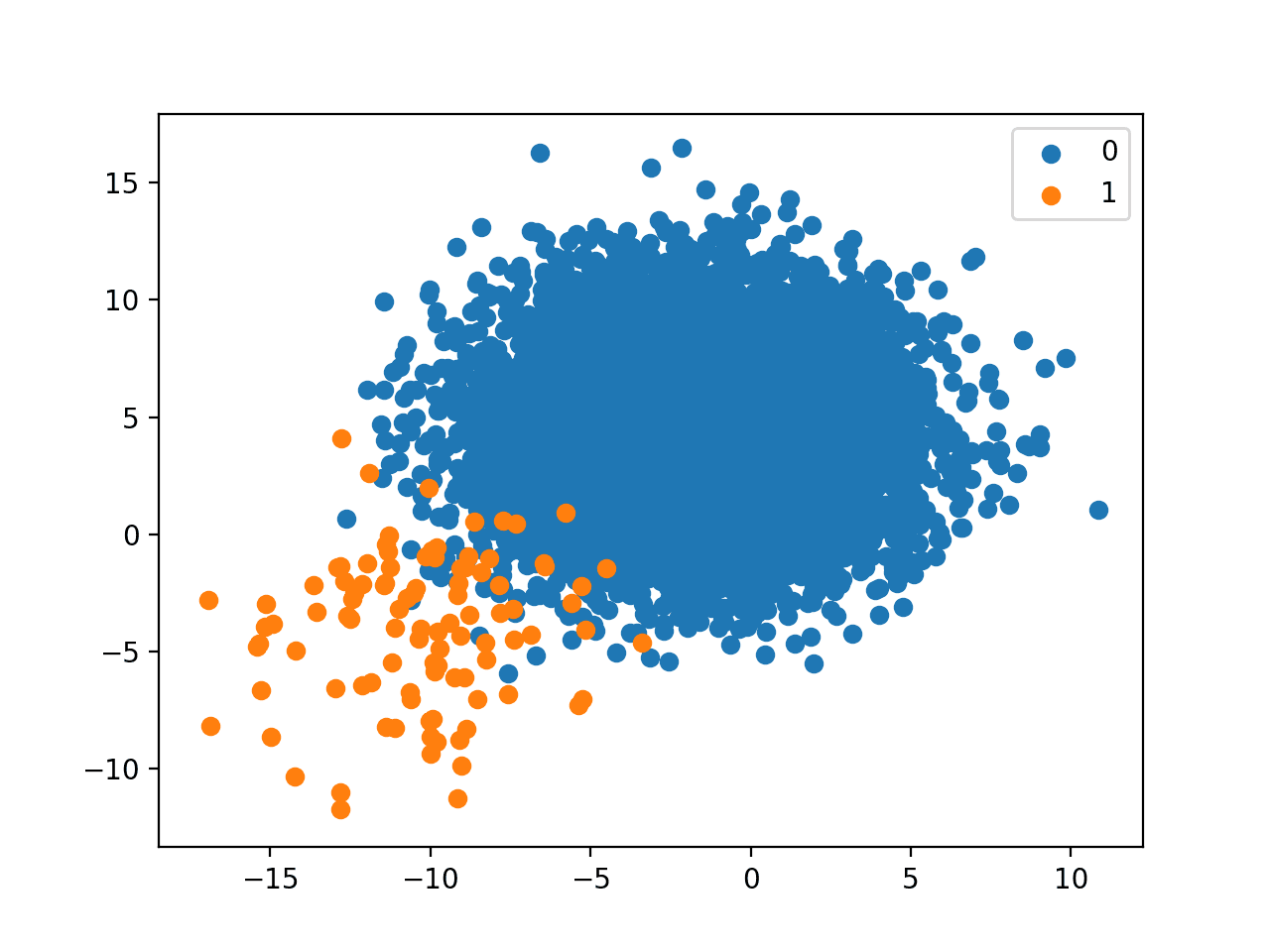
A plot of the dataset is created and we can see that there are many more examples for each class and a helpful legend to indicate the mapping of plot colors to class labels.

Scatter Plot of Binary Classification Dataset With 1 to 100 Class Distribution

Next, we can fit a naive classifier model that always predicts the majority class.

We can achieve this using the DummyClassifier from scikit-learn and use the ‘most_frequent‘ strategy that will always predict the class label that is most observed in the training dataset.

We can then evaluate this model on the training dataset using repeated k-fold cross-validation. It is important that we use stratified cross-validation to ensure that each split of the dataset has the same class distribution as the training dataset. This can be achieved using the RepeatedStratifiedKFold class.

The evaluate_model() function below implements this and returns a list of scores for each evaluation of the model.

We can then evaluate the model and calculate the mean of the scores across each evaluation.

We would expect that the naive classifier would achieve a classification accuracy of about 99 percent, which we know because that is the distribution of the majority class in the training dataset.

Tying this all together, the complete example of evaluating a naive classifier on the synthetic dataset with a 1:100 class distribution is listed below.

Running the example first reports the class distribution of the training dataset again.

Then the model is evaluated and the mean accuracy is reported. We can see that as expected, the performance of the naive classifier matches the class distribution exactly.

Normally, achieving 99 percent classification accuracy would be cause for celebration. Although, as we have seen, because the class distribution is imbalanced, 99 percent is actually the lowest acceptable accuracy for this dataset and the starting point from which more sophisticated models must improve.

Further Reading

This section provides more resources on the topic if you are looking to go deeper.

Tutorials

• What is a Confusion Matrix in Machine Learning

Papers

• A Survey of Predictive Modelling under Imbalanced Distributions, 2015.
• A Review on Ensembles for the Class Imbalance Problem: Bagging-, Boosting-, and Hybrid-Based Approaches, 2011.

Books

• Imbalanced Learning: Foundations, Algorithms, and Applications, 2013.
• Learning from Imbalanced Data Sets, 2018.

APIs

• sklearn.datasets.make_blobs API.
• sklearn.dummy.DummyClassifier API.
• sklearn.model_selection.RepeatedStratifiedKFold API.

Articles

• Accuracy and precision, Wikipedia.
• Accuracy paradox, Wikipedia.

Summary

In this tutorial, you discovered the failure of classification accuracy for imbalanced classification problems.

Specifically, you learned:

• Accuracy and error rate are the de facto standard metrics for summarizing the performance of classification models.
• Classification accuracy fails on classification problems with a skewed class distribution because of the intuitions developed by practitioners on datasets with an equal class distribution.
• Intuition for the failure of accuracy for skewed class distributions with a worked example.

Do you have any questions?
Ask your questions in the comments below and I will do my best to answer.

Get a Handle on Imbalanced Classification!

Develop Imbalanced Learning Models in Minutes

...with just a few lines of python code

Discover how in my new Ebook:
Imbalanced Classification with Python

It provides self-study tutorials and end-to-end projects on:
Performance Metrics, Undersampling Methods, SMOTE, Threshold Moving, Probability Calibration, Cost-Sensitive Algorithms
and much more...

Bring Imbalanced Classification Methods to Your Machine Learning Projects

See What's Inside