How to Identify Unstable Models When Training Generative Adversarial Networks.
GANs are difficult to train.
The reason they are difficult to train is that both the generator model and the discriminator model are trained simultaneously in a zero sum game. This means that improvements to one model come at the expense of the other model.
The goal of training two models involves finding a point of equilibrium between the two competing concerns.
It also means that every time the parameters of one of the models are updated, the nature of the optimization problem that is being solved is changed. This has the effect of creating a dynamic system. In neural network terms, the technical challenge of training two competing neural networks at the same time is that they can fail to converge.
It is important to develop an intuition for both the normal convergence of a GAN model and unusual convergence of GAN models, sometimes called failure modes.
In this tutorial, we will first develop a stable GAN model for a simple image generation task in order to establish what normal convergence looks like and what to expect more generally.
We will then impair the GAN models in different ways and explore a range of failure modes that you may encounter when training GAN models. These scenarios will help you to develop an intuition for what to look for or expect when a GAN model is failing to train, and ideas for what you could do about it.
After completing this tutorial, you will know:
- How to identify a stable GAN training process from the generator and discriminator loss over time.
- How to identify a mode collapse by reviewing both learning curves and generated images.
- How to identify a convergence failure by reviewing learning curves of generator and discriminator loss over time.
Kick-start your project with my new book Generative Adversarial Networks with Python, including step-by-step tutorials and the Python source code files for all examples.
Let’s get started.
- Updated Aug/2020: Corrected label on line plot.
- Updated Jan/2021: Updated so layer freezing works with batch norm.
- Updated Jan/2021: Simplified model architecture to ensure we see failures.
A Practical Guide to Generative Adversarial Network Failure Modes
Photo by Jason Heavner, some rights reserved.
Tutorial Overview
This tutorial is divided into three parts; they are:
- How To Identify a Stable Generative Adversarial Network
- How To Identify a Mode Collapse in a Generative Adversarial Network
- How To Identify Convergence Failure in a Generative Adversarial Network
How To Train a Stable Generative Adversarial Network
In this section, we will train a stable GAN to generate images of a handwritten digit.
Specifically, we will use the digit ‘8’ from the MNIST handwritten digit dataset.
The results of this model will establish both a stable GAN that can be used for later experimentation and a profile for what generated images and learning curves look like for a stable GAN training process.
The first step is to define the models.
The discriminator model takes as input one 28×28 grayscale image and outputs a binary prediction as to whether the image is real (class=1) or fake (class=0). It is implemented as a modest convolutional neural network using best practices for GAN design such as using the LeakyReLU activation function with a slope of 0.2, a 2×2 stride to downsample, and the adam version of stochastic gradient descent with a learning rate of 0.0002 and a momentum of 0.5
The define_discriminator() function below implements this, defining and compiling the discriminator model and returning it. The input shape of the image is parameterized as a default function argument to make it clear.
|
1 2 3 4 5 6 7 8 9 10 11 12 13 14 15 16 17 18 19 |
# define the standalone discriminator model def define_discriminator(in_shape=(28,28,1)): # weight initialization init = RandomNormal(stddev=0.02) # define model model = Sequential() # downsample to 14x14 model.add(Conv2D(64, (4,4), strides=(2,2), padding='same', kernel_initializer=init, input_shape=in_shape)) model.add(LeakyReLU(alpha=0.2)) # downsample to 7x7 model.add(Conv2D(64, (4,4), strides=(2,2), padding='same', kernel_initializer=init)) model.add(LeakyReLU(alpha=0.2)) # classifier model.add(Flatten()) model.add(Dense(1, activation='sigmoid')) # compile model opt = Adam(lr=0.0002, beta_1=0.5) model.compile(loss='binary_crossentropy', optimizer=opt, metrics=['accuracy']) return model |
The generator model takes as input a point in the latent space and outputs a single 28×28 grayscale image. This is achieved by using a fully connected layer to interpret the point in the latent space and provide sufficient activations that can be reshaped into many copies (in this case, 128) of a low-resolution version of the output image (e.g. 7×7). This is then upsampled two times, doubling the size and quadrupling the area of the activations each time using transpose convolutional layers. The model uses best practices such as the LeakyReLU activation, a kernel size that is a factor of the stride size, and a hyperbolic tangent (tanh) activation function in the output layer.
Want to Develop GANs from Scratch?
Take my free 7-day email crash course now (with sample code).
Click to sign-up and also get a free PDF Ebook version of the course.
The define_generator() function below defines the generator model, but intentionally does not compile it as it is not trained directly, then returns the model. The size of the latent space is parameterized as a function argument.
|
1 2 3 4 5 6 7 8 9 10 11 12 13 14 15 16 17 18 19 20 |
# define the standalone generator model def define_generator(latent_dim): # weight initialization init = RandomNormal(stddev=0.02) # define model model = Sequential() # foundation for 7x7 image n_nodes = 128 * 7 * 7 model.add(Dense(n_nodes, kernel_initializer=init, input_dim=latent_dim)) model.add(LeakyReLU(alpha=0.2)) model.add(Reshape((7, 7, 128))) # upsample to 14x14 model.add(Conv2DTranspose(128, (4,4), strides=(2,2), padding='same', kernel_initializer=init)) model.add(LeakyReLU(alpha=0.2)) # upsample to 28x28 model.add(Conv2DTranspose(128, (4,4), strides=(2,2), padding='same', kernel_initializer=init)) model.add(LeakyReLU(alpha=0.2)) # output 28x28x1 model.add(Conv2D(1, (7,7), activation='tanh', padding='same', kernel_initializer=init)) return model |
Next, a GAN model can be defined that combines both the generator model and the discriminator model into one larger model. This larger model will be used to train the model weights in the generator, using the output and error calculated by the discriminator model. The discriminator model is trained separately, and as such, the model weights are marked as not trainable in this larger GAN model to ensure that only the weights of the generator model are updated. This change to the trainability of the discriminator weights only has an effect when training the combined GAN model, not when training the discriminator standalone.
This larger GAN model takes as input a point in the latent space, uses the generator model to generate an image, which is fed as input to the discriminator model, then output or classified as real or fake.
The define_gan() function below implements this, taking the already defined generator and discriminator models as input.
|
1 2 3 4 5 6 7 8 9 10 11 12 13 14 |
# define the combined generator and discriminator model, for updating the generator def define_gan(generator, discriminator): # make weights in the discriminator not trainable discriminator.trainable = False # connect them model = Sequential() # add generator model.add(generator) # add the discriminator model.add(discriminator) # compile model opt = Adam(lr=0.0002, beta_1=0.5) model.compile(loss='binary_crossentropy', optimizer=opt) return model |
Now that we have defined the GAN model, we need to train it. But, before we can train the model, we require input data.
The first step is to load and scale the MNIST dataset. The whole dataset is loaded via a call to the load_data() Keras function, then a subset of the images are selected (about 5,000) that belong to class 8, e.g. are a handwritten depiction of the number eight. Then the pixel values must be scaled to the range [-1,1] to match the output of the generator model.
The load_real_samples() function below implements this, returning the loaded and scaled subset of the MNIST training dataset ready for modeling.
|
1 2 3 4 5 6 7 8 9 10 11 12 13 14 |
# load mnist images def load_real_samples(): # load dataset (trainX, trainy), (_, _) = load_data() # expand to 3d, e.g. add channels X = expand_dims(trainX, axis=-1) # select all of the examples for a given class selected_ix = trainy == 8 X = X[selected_ix] # convert from ints to floats X = X.astype('float32') # scale from [0,255] to [-1,1] X = (X - 127.5) / 127.5 return X |
We will require one (or a half) batch of real images from the dataset each update to the GAN model. A simple way to achieve this is to select a random sample of images from the dataset each time.
The generate_real_samples() function below implements this, taking the prepared dataset as an argument, selecting and returning a random sample of face images, and their corresponding class label for the discriminator, specifically class=1 indicating that they are real images.
|
1 2 3 4 5 6 7 8 9 |
# select real samples def generate_real_samples(dataset, n_samples): # choose random instances ix = randint(0, dataset.shape[0], n_samples) # select images X = dataset[ix] # generate class labels y = ones((n_samples, 1)) return X, y |
Next, we need inputs for the generator model. These are random points from the latent space, specifically Gaussian distributed random variables.
The generate_latent_points() function implements this, taking the size of the latent space as an argument and the number of points required, and returning them as a batch of input samples for the generator model.
|
1 2 3 4 5 6 7 |
# generate points in latent space as input for the generator def generate_latent_points(latent_dim, n_samples): # generate points in the latent space x_input = randn(latent_dim * n_samples) # reshape into a batch of inputs for the network x_input = x_input.reshape(n_samples, latent_dim) return x_input |
Next, we need to use the points in the latent space as input to the generator in order to generate new images.
The generate_fake_samples() function below implements this, taking the generator model and size of the latent space as arguments, then generating points in the latent space and using them as input to the generator model. The function returns the generated images and their corresponding class label for the discriminator model, specifically class=0 to indicate they are fake or generated.
|
1 2 3 4 5 6 7 8 9 |
# use the generator to generate n fake examples, with class labels def generate_fake_samples(generator, latent_dim, n_samples): # generate points in latent space x_input = generate_latent_points(latent_dim, n_samples) # predict outputs X = generator.predict(x_input) # create class labels y = zeros((n_samples, 1)) return X, y |
We need to record the performance of the model. Perhaps the most reliable way to evaluate the performance of a GAN is to use the generator to generate images, and then review and subjectively evaluate them.
The summarize_performance() function below takes the generator model at a given point during training and uses it to generate 100 images in a 10×10 grid that are then plotted and saved to file. The model is also saved to file at this time, in case we would like to use it later to generate more images.
|
1 2 3 4 5 6 7 8 9 10 11 12 13 14 15 16 17 18 19 |
# generate samples and save as a plot and save the model def summarize_performance(step, g_model, latent_dim, n_samples=100): # prepare fake examples X, _ = generate_fake_samples(g_model, latent_dim, n_samples) # scale from [-1,1] to [0,1] X = (X + 1) / 2.0 # plot images for i in range(10 * 10): # define subplot pyplot.subplot(10, 10, 1 + i) # turn off axis pyplot.axis('off') # plot raw pixel data pyplot.imshow(X[i, :, :, 0], cmap='gray_r') # save plot to file pyplot.savefig('results_baseline/generated_plot_%03d.png' % (step+1)) pyplot.close() # save the generator model g_model.save('results_baseline/model_%03d.h5' % (step+1)) |
In addition to image quality, it is a good idea to keep track of the loss and accuracy of the model over time.
The loss and classification accuracy for the discriminator for real and fake samples can be tracked for each model update, as can the loss for the generator for each update. These can then be used to create line plots of loss and accuracy at the end of the training run.
The plot_history() function below implements this and saves the results to file.
|
1 2 3 4 5 6 7 8 9 10 11 12 13 14 15 16 |
# create a line plot of loss for the gan and save to file def plot_history(d1_hist, d2_hist, g_hist, a1_hist, a2_hist): # plot loss pyplot.subplot(2, 1, 1) pyplot.plot(d1_hist, label='d-real') pyplot.plot(d2_hist, label='d-fake') pyplot.plot(g_hist, label='gen') pyplot.legend() # plot discriminator accuracy pyplot.subplot(2, 1, 2) pyplot.plot(a1_hist, label='acc-real') pyplot.plot(a2_hist, label='acc-fake') pyplot.legend() # save plot to file pyplot.savefig('results_baseline/plot_line_plot_loss.png') pyplot.close() |
We are now ready to fit the GAN model.
The model is fit for 10 training epochs, which is arbitrary, as the model begins generating plausible number-8 digits after perhaps the first few epochs. A batch size of 128 samples is used, and each training epoch involves 5,851/128 or about 45 batches of real and fake samples and updates to the model. The model is therefore trained for 10 epochs of 45 batches, or 450 iterations.
First, the discriminator model is updated for a half batch of real samples, then a half batch of fake samples, together forming one batch of weight updates. The generator is then updated via the composite GAN model. Importantly, the class label is set to 1, or real, for the fake samples. This has the effect of updating the generator toward getting better at generating real samples on the next batch.
The train() function below implements this, taking the defined models, dataset, and size of the latent dimension as arguments and parameterizing the number of epochs and batch size with default arguments. The generator model is saved at the end of training.
The performance of the discriminator and generator models is reported each iteration. Sample images are generated and saved every epoch, and line plots of model performance are created and saved at the end of the run.
|
1 2 3 4 5 6 7 8 9 10 11 12 13 14 15 16 17 18 19 20 21 22 23 24 25 26 27 28 29 30 31 32 33 34 35 36 37 38 39 |
# train the generator and discriminator def train(g_model, d_model, gan_model, dataset, latent_dim, n_epochs=10, n_batch=128): # calculate the number of batches per epoch bat_per_epo = int(dataset.shape[0] / n_batch) # calculate the total iterations based on batch and epoch n_steps = bat_per_epo * n_epochs # calculate the number of samples in half a batch half_batch = int(n_batch / 2) # prepare lists for storing stats each iteration d1_hist, d2_hist, g_hist, a1_hist, a2_hist = list(), list(), list(), list(), list() # manually enumerate epochs for i in range(n_steps): # get randomly selected 'real' samples X_real, y_real = generate_real_samples(dataset, half_batch) # update discriminator model weights d_loss1, d_acc1 = d_model.train_on_batch(X_real, y_real) # generate 'fake' examples X_fake, y_fake = generate_fake_samples(g_model, latent_dim, half_batch) # update discriminator model weights d_loss2, d_acc2 = d_model.train_on_batch(X_fake, y_fake) # prepare points in latent space as input for the generator X_gan = generate_latent_points(latent_dim, n_batch) # create inverted labels for the fake samples y_gan = ones((n_batch, 1)) # update the generator via the discriminator's error g_loss = gan_model.train_on_batch(X_gan, y_gan) # summarize loss on this batch print('>%d, d1=%.3f, d2=%.3f g=%.3f, a1=%d, a2=%d' % (i+1, d_loss1, d_loss2, g_loss, int(100*d_acc1), int(100*d_acc2))) # record history d1_hist.append(d_loss1) d2_hist.append(d_loss2) g_hist.append(g_loss) a1_hist.append(d_acc1) a2_hist.append(d_acc2) # evaluate the model performance every 'epoch' if (i+1) % bat_per_epo == 0: summarize_performance(i, g_model, latent_dim) plot_history(d1_hist, d2_hist, g_hist, a1_hist, a2_hist) |
Now that all of the functions have been defined, we can create the directory where images and models will be stored (in this case ‘results_baseline‘), create the models, load the dataset, and begin the training process.
|
1 2 3 4 5 6 7 8 9 10 11 12 13 14 15 |
# make folder for results makedirs('results_baseline', exist_ok=True) # size of the latent space latent_dim = 50 # create the discriminator discriminator = define_discriminator() # create the generator generator = define_generator(latent_dim) # create the gan gan_model = define_gan(generator, discriminator) # load image data dataset = load_real_samples() print(dataset.shape) # train model train(generator, discriminator, gan_model, dataset, latent_dim) |
Tying all of this together, the complete example is listed below.
|
1 2 3 4 5 6 7 8 9 10 11 12 13 14 15 16 17 18 19 20 21 22 23 24 25 26 27 28 29 30 31 32 33 34 35 36 37 38 39 40 41 42 43 44 45 46 47 48 49 50 51 52 53 54 55 56 57 58 59 60 61 62 63 64 65 66 67 68 69 70 71 72 73 74 75 76 77 78 79 80 81 82 83 84 85 86 87 88 89 90 91 92 93 94 95 96 97 98 99 100 101 102 103 104 105 106 107 108 109 110 111 112 113 114 115 116 117 118 119 120 121 122 123 124 125 126 127 128 129 130 131 132 133 134 135 136 137 138 139 140 141 142 143 144 145 146 147 148 149 150 151 152 153 154 155 156 157 158 159 160 161 162 163 164 165 166 167 168 169 170 171 172 173 174 175 176 177 178 179 180 181 182 183 184 185 186 187 188 189 190 191 192 193 194 195 196 197 198 199 200 201 202 203 204 205 206 207 208 209 210 |
# example of training a stable gan for generating a handwritten digit from os import makedirs from numpy import expand_dims from numpy import zeros from numpy import ones from numpy.random import randn from numpy.random import randint from keras.datasets.mnist import load_data from keras.optimizers import Adam from keras.models import Sequential from keras.layers import Dense from keras.layers import Reshape from keras.layers import Flatten from keras.layers import Conv2D from keras.layers import Conv2DTranspose from keras.layers import LeakyReLU from keras.initializers import RandomNormal from matplotlib import pyplot # define the standalone discriminator model def define_discriminator(in_shape=(28,28,1)): # weight initialization init = RandomNormal(stddev=0.02) # define model model = Sequential() # downsample to 14x14 model.add(Conv2D(64, (4,4), strides=(2,2), padding='same', kernel_initializer=init, input_shape=in_shape)) model.add(LeakyReLU(alpha=0.2)) # downsample to 7x7 model.add(Conv2D(64, (4,4), strides=(2,2), padding='same', kernel_initializer=init)) model.add(LeakyReLU(alpha=0.2)) # classifier model.add(Flatten()) model.add(Dense(1, activation='sigmoid')) # compile model opt = Adam(lr=0.0002, beta_1=0.5) model.compile(loss='binary_crossentropy', optimizer=opt, metrics=['accuracy']) return model # define the standalone generator model def define_generator(latent_dim): # weight initialization init = RandomNormal(stddev=0.02) # define model model = Sequential() # foundation for 7x7 image n_nodes = 128 * 7 * 7 model.add(Dense(n_nodes, kernel_initializer=init, input_dim=latent_dim)) model.add(LeakyReLU(alpha=0.2)) model.add(Reshape((7, 7, 128))) # upsample to 14x14 model.add(Conv2DTranspose(128, (4,4), strides=(2,2), padding='same', kernel_initializer=init)) model.add(LeakyReLU(alpha=0.2)) # upsample to 28x28 model.add(Conv2DTranspose(128, (4,4), strides=(2,2), padding='same', kernel_initializer=init)) model.add(LeakyReLU(alpha=0.2)) # output 28x28x1 model.add(Conv2D(1, (7,7), activation='tanh', padding='same', kernel_initializer=init)) return model # define the combined generator and discriminator model, for updating the generator def define_gan(generator, discriminator): # make weights in the discriminator not trainable discriminator.trainable = False # connect them model = Sequential() # add generator model.add(generator) # add the discriminator model.add(discriminator) # compile model opt = Adam(lr=0.0002, beta_1=0.5) model.compile(loss='binary_crossentropy', optimizer=opt) return model # load mnist images def load_real_samples(): # load dataset (trainX, trainy), (_, _) = load_data() # expand to 3d, e.g. add channels X = expand_dims(trainX, axis=-1) # select all of the examples for a given class selected_ix = trainy == 8 X = X[selected_ix] # convert from ints to floats X = X.astype('float32') # scale from [0,255] to [-1,1] X = (X - 127.5) / 127.5 return X # select real samples def generate_real_samples(dataset, n_samples): # choose random instances ix = randint(0, dataset.shape[0], n_samples) # select images X = dataset[ix] # generate class labels y = ones((n_samples, 1)) return X, y # generate points in latent space as input for the generator def generate_latent_points(latent_dim, n_samples): # generate points in the latent space x_input = randn(latent_dim * n_samples) # reshape into a batch of inputs for the network x_input = x_input.reshape(n_samples, latent_dim) return x_input # use the generator to generate n fake examples, with class labels def generate_fake_samples(generator, latent_dim, n_samples): # generate points in latent space x_input = generate_latent_points(latent_dim, n_samples) # predict outputs X = generator.predict(x_input) # create class labels y = zeros((n_samples, 1)) return X, y # generate samples and save as a plot and save the model def summarize_performance(step, g_model, latent_dim, n_samples=100): # prepare fake examples X, _ = generate_fake_samples(g_model, latent_dim, n_samples) # scale from [-1,1] to [0,1] X = (X + 1) / 2.0 # plot images for i in range(10 * 10): # define subplot pyplot.subplot(10, 10, 1 + i) # turn off axis pyplot.axis('off') # plot raw pixel data pyplot.imshow(X[i, :, :, 0], cmap='gray_r') # save plot to file pyplot.savefig('results_baseline/generated_plot_%03d.png' % (step+1)) pyplot.close() # save the generator model g_model.save('results_baseline/model_%03d.h5' % (step+1)) # create a line plot of loss for the gan and save to file def plot_history(d1_hist, d2_hist, g_hist, a1_hist, a2_hist): # plot loss pyplot.subplot(2, 1, 1) pyplot.plot(d1_hist, label='d-real') pyplot.plot(d2_hist, label='d-fake') pyplot.plot(g_hist, label='gen') pyplot.legend() # plot discriminator accuracy pyplot.subplot(2, 1, 2) pyplot.plot(a1_hist, label='acc-real') pyplot.plot(a2_hist, label='acc-fake') pyplot.legend() # save plot to file pyplot.savefig('results_baseline/plot_line_plot_loss.png') pyplot.close() # train the generator and discriminator def train(g_model, d_model, gan_model, dataset, latent_dim, n_epochs=10, n_batch=128): # calculate the number of batches per epoch bat_per_epo = int(dataset.shape[0] / n_batch) # calculate the total iterations based on batch and epoch n_steps = bat_per_epo * n_epochs # calculate the number of samples in half a batch half_batch = int(n_batch / 2) # prepare lists for storing stats each iteration d1_hist, d2_hist, g_hist, a1_hist, a2_hist = list(), list(), list(), list(), list() # manually enumerate epochs for i in range(n_steps): # get randomly selected 'real' samples X_real, y_real = generate_real_samples(dataset, half_batch) # update discriminator model weights d_loss1, d_acc1 = d_model.train_on_batch(X_real, y_real) # generate 'fake' examples X_fake, y_fake = generate_fake_samples(g_model, latent_dim, half_batch) # update discriminator model weights d_loss2, d_acc2 = d_model.train_on_batch(X_fake, y_fake) # prepare points in latent space as input for the generator X_gan = generate_latent_points(latent_dim, n_batch) # create inverted labels for the fake samples y_gan = ones((n_batch, 1)) # update the generator via the discriminator's error g_loss = gan_model.train_on_batch(X_gan, y_gan) # summarize loss on this batch print('>%d, d1=%.3f, d2=%.3f g=%.3f, a1=%d, a2=%d' % (i+1, d_loss1, d_loss2, g_loss, int(100*d_acc1), int(100*d_acc2))) # record history d1_hist.append(d_loss1) d2_hist.append(d_loss2) g_hist.append(g_loss) a1_hist.append(d_acc1) a2_hist.append(d_acc2) # evaluate the model performance every 'epoch' if (i+1) % bat_per_epo == 0: summarize_performance(i, g_model, latent_dim) plot_history(d1_hist, d2_hist, g_hist, a1_hist, a2_hist) # make folder for results makedirs('results_baseline', exist_ok=True) # size of the latent space latent_dim = 50 # create the discriminator discriminator = define_discriminator() # create the generator generator = define_generator(latent_dim) # create the gan gan_model = define_gan(generator, discriminator) # load image data dataset = load_real_samples() print(dataset.shape) # train model train(generator, discriminator, gan_model, dataset, latent_dim) |
Running the example is quick, taking approximately 10 minutes on modern hardware without a GPU.
Your specific results will vary given the stochastic nature of the learning algorithm. Nevertheless, the general structure of training should be very similar.
First, the loss and accuracy of the discriminator and loss for the generator model are reported to the console each iteration of the training loop.
This is important. A stable GAN will have a discriminator loss around 0.5, typically between 0.5 and maybe as high as 0.7 or 0.8. The generator loss is typically higher and may hover around 1.0, 1.5, 2.0, or even higher.
The accuracy of the discriminator on both real and generated (fake) images will not be 50%, but should typically hover around 70% to 80%.
For both the discriminator and generator, behaviors are likely to start off erratic and move around a lot before the model converges to a stable equilibrium.
|
1 2 3 4 5 6 7 8 9 10 11 |
>1, d1=0.859, d2=0.664 g=0.872, a1=37, a2=59 >2, d1=0.190, d2=1.429 g=0.555, a1=100, a2=10 >3, d1=0.094, d2=1.467 g=0.597, a1=100, a2=4 >4, d1=0.097, d2=1.315 g=0.686, a1=100, a2=9 >5, d1=0.100, d2=1.241 g=0.714, a1=100, a2=9 ... >446, d1=0.593, d2=0.546 g=1.330, a1=76, a2=82 >447, d1=0.551, d2=0.739 g=0.981, a1=82, a2=39 >448, d1=0.628, d2=0.505 g=1.420, a1=79, a2=89 >449, d1=0.641, d2=0.533 g=1.381, a1=60, a2=85 >450, d1=0.550, d2=0.731 g=1.100, a1=76, a2=42 |
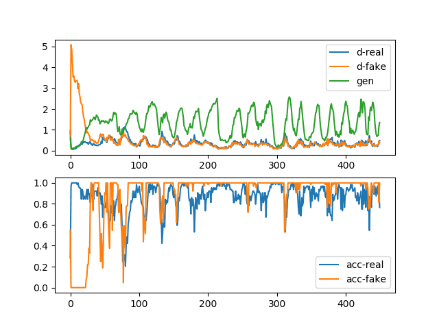
Line plots for loss and accuracy are created and saved at the end of the run.
The figure contains two subplots. The top subplot shows line plots for the discriminator loss for real images (blue), discriminator loss for generated fake images (orange), and the generator loss for generated fake images (green).
We can see that all three losses are somewhat erratic early in the run before stabilizing around epoch 100 to epoch 300. Losses remain stable after that, although the variance increases.
This is an example of the normal or expected loss during training. Namely, discriminator loss for real and fake samples is about the same at or around 0.5, and loss for the generator is slightly higher between 0.5 and 2.0. If the generator model is capable of generating plausible images, then the expectation is that those images would have been generated between epochs 100 and 300 and likely between 300 and 450 as well.
The bottom subplot shows a line plot of the discriminator accuracy on real (blue) and fake (orange) images during training. We see a similar structure as the subplot of loss, namely that accuracy starts off quite different between the two image types, then stabilizes between epochs 100 to 300 at around 70% to 80%, and remains stable beyond that, although with increased variance.
The time scales (e.g. number of iterations or training epochs) for these patterns and absolute values will vary across problems and types of GAN models, although the plot provides a good baseline for what to expect when training a stable GAN model.
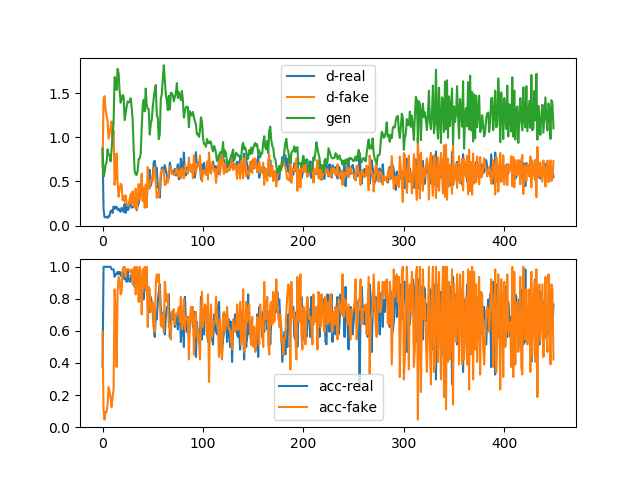
Line Plots of Loss and Accuracy for a Stable Generative Adversarial Network
Finally, we can review samples of generated images. Note: we are generating images using a reverse grayscale color map, meaning that the normal white figure on a background is inverted to a black figure on a white background. This was done to make the generated figures easier to review.
As we might expect, samples of images generated before epoch 100 are relatively poor in quality.
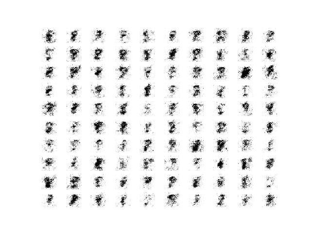
Sample of 100 Generated Images of a Handwritten Number 8 at Epoch 45 From a Stable GAN.
Samples of images generated between epochs 100 and 300 are plausible, and perhaps the best quality.
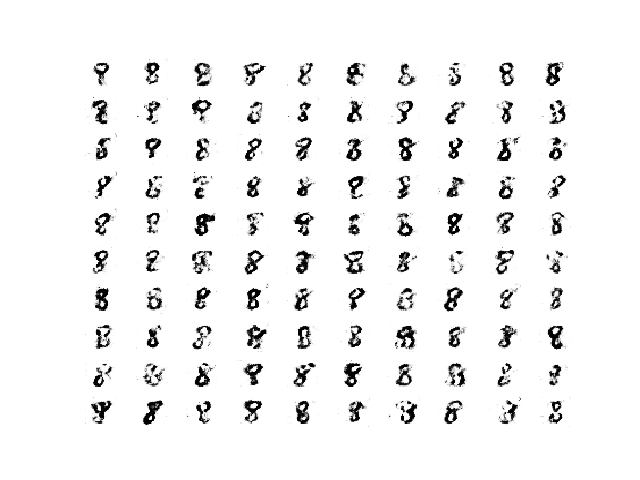
Sample of 100 Generated Images of a Handwritten Number 8 at Epoch 180 From a Stable GAN.
And samples of generated images after epoch 300 remain plausible, although perhaps have more noise, e.g. background noise.
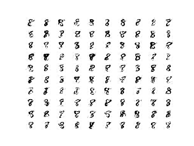
Sample of 100 Generated Images of a Handwritten Number 8 at Epoch 450 From a Stable GAN.
These results are important, as it highlights that the quality generated can and does vary across the run, even after the training process becomes stable.
More training iterations, beyond some point of training stability may or may not result in higher quality images.
We can summarize these observations for stable GAN training as follows:
- Discriminator loss on real and fake images is expected to sit around 0.5.
- Generator loss on fake images is expected to sit between 0.5 and perhaps 2.0.
- Discriminator accuracy on real and fake images is expected to sit around 80%.
- Variance of generator and discriminator loss is expected to remain modest.
- The generator is expected to produce its highest quality images during a period of stability.
- Training stability may degenerate into periods of high-variance loss and corresponding lower quality generated images.
Now that we have a stable GAN model, we can look into modifying it to produce some specific failure cases.
There are two failure cases that are common to see when training GAN models on new problems; they are mode collapse and convergence failure.
How To Identify a Mode Collapse in a Generative Adversarial Network
A mode collapse refers to a generator model that is only capable of generating one or a small subset of different outcomes, or modes.
Here, mode refers to an output distribution, e.g. a multi-modal function refers to a function with more than one peak or optima. With a GAN generator model, a mode failure means that the vast number of points in the input latent space (e.g. hypersphere of 100 dimensions in many cases) result in one or a small subset of generated images.
Mode collapse, also known as the scenario, is a problem that occurs when the generator learns to map several different input z values to the same output point.
— NIPS 2016 Tutorial: Generative Adversarial Networks, 2016.
A mode collapse can be identified when reviewing a large sample of generated images. The images will show low diversity, with the same identical image or same small subset of identical images repeating many times.
A mode collapse can also be identified by reviewing the line plot of model loss. The line plot will show oscillations in the loss over time, most notably in the generator model, as the generator model is updated and jumps from generating one mode to another model that has different loss.
We can impair our stable GAN to suffer mode collapse a number of ways. Perhaps the most reliable is to restrict the size of the latent dimension directly, forcing the model to only generate a small subset of plausible outputs.
Specifically, the ‘latent_dim‘ variable can be changed from 100 to 1, and the experiment re-run.
|
1 2 |
# size of the latent space latent_dim = 1 |
The full code listing is provided below for completeness.
|
1 2 3 4 5 6 7 8 9 10 11 12 13 14 15 16 17 18 19 20 21 22 23 24 25 26 27 28 29 30 31 32 33 34 35 36 37 38 39 40 41 42 43 44 45 46 47 48 49 50 51 52 53 54 55 56 57 58 59 60 61 62 63 64 65 66 67 68 69 70 71 72 73 74 75 76 77 78 79 80 81 82 83 84 85 86 87 88 89 90 91 92 93 94 95 96 97 98 99 100 101 102 103 104 105 106 107 108 109 110 111 112 113 114 115 116 117 118 119 120 121 122 123 124 125 126 127 128 129 130 131 132 133 134 135 136 137 138 139 140 141 142 143 144 145 146 147 148 149 150 151 152 153 154 155 156 157 158 159 160 161 162 163 164 165 166 167 168 169 170 171 172 173 174 175 176 177 178 179 180 181 182 183 184 185 186 187 188 189 190 191 192 193 194 195 196 197 198 199 200 201 202 203 204 205 206 207 208 209 210 |
# example of training an unstable gan for generating a handwritten digit from os import makedirs from numpy import expand_dims from numpy import zeros from numpy import ones from numpy.random import randn from numpy.random import randint from keras.datasets.mnist import load_data from keras.optimizers import Adam from keras.models import Sequential from keras.layers import Dense from keras.layers import Reshape from keras.layers import Flatten from keras.layers import Conv2D from keras.layers import Conv2DTranspose from keras.layers import LeakyReLU from keras.initializers import RandomNormal from matplotlib import pyplot # define the standalone discriminator model def define_discriminator(in_shape=(28,28,1)): # weight initialization init = RandomNormal(stddev=0.02) # define model model = Sequential() # downsample to 14x14 model.add(Conv2D(64, (4,4), strides=(2,2), padding='same', kernel_initializer=init, input_shape=in_shape)) model.add(LeakyReLU(alpha=0.2)) # downsample to 7x7 model.add(Conv2D(64, (4,4), strides=(2,2), padding='same', kernel_initializer=init)) model.add(LeakyReLU(alpha=0.2)) # classifier model.add(Flatten()) model.add(Dense(1, activation='sigmoid')) # compile model opt = Adam(lr=0.0002, beta_1=0.5) model.compile(loss='binary_crossentropy', optimizer=opt, metrics=['accuracy']) return model # define the standalone generator model def define_generator(latent_dim): # weight initialization init = RandomNormal(stddev=0.02) # define model model = Sequential() # foundation for 7x7 image n_nodes = 128 * 7 * 7 model.add(Dense(n_nodes, kernel_initializer=init, input_dim=latent_dim)) model.add(LeakyReLU(alpha=0.2)) model.add(Reshape((7, 7, 128))) # upsample to 14x14 model.add(Conv2DTranspose(128, (4,4), strides=(2,2), padding='same', kernel_initializer=init)) model.add(LeakyReLU(alpha=0.2)) # upsample to 28x28 model.add(Conv2DTranspose(128, (4,4), strides=(2,2), padding='same', kernel_initializer=init)) model.add(LeakyReLU(alpha=0.2)) # output 28x28x1 model.add(Conv2D(1, (7,7), activation='tanh', padding='same', kernel_initializer=init)) return model # define the combined generator and discriminator model, for updating the generator def define_gan(generator, discriminator): # make weights in the discriminator not trainable discriminator.trainable = False # connect them model = Sequential() # add generator model.add(generator) # add the discriminator model.add(discriminator) # compile model opt = Adam(lr=0.0002, beta_1=0.5) model.compile(loss='binary_crossentropy', optimizer=opt) return model # load mnist images def load_real_samples(): # load dataset (trainX, trainy), (_, _) = load_data() # expand to 3d, e.g. add channels X = expand_dims(trainX, axis=-1) # select all of the examples for a given class selected_ix = trainy == 8 X = X[selected_ix] # convert from ints to floats X = X.astype('float32') # scale from [0,255] to [-1,1] X = (X - 127.5) / 127.5 return X # # select real samples def generate_real_samples(dataset, n_samples): # choose random instances ix = randint(0, dataset.shape[0], n_samples) # select images X = dataset[ix] # generate class labels y = ones((n_samples, 1)) return X, y # generate points in latent space as input for the generator def generate_latent_points(latent_dim, n_samples): # generate points in the latent space x_input = randn(latent_dim * n_samples) # reshape into a batch of inputs for the network x_input = x_input.reshape(n_samples, latent_dim) return x_input # use the generator to generate n fake examples, with class labels def generate_fake_samples(generator, latent_dim, n_samples): # generate points in latent space x_input = generate_latent_points(latent_dim, n_samples) # predict outputs X = generator.predict(x_input) # create class labels y = zeros((n_samples, 1)) return X, y # generate samples and save as a plot and save the model def summarize_performance(step, g_model, latent_dim, n_samples=100): # prepare fake examples X, _ = generate_fake_samples(g_model, latent_dim, n_samples) # scale from [-1,1] to [0,1] X = (X + 1) / 2.0 # plot images for i in range(10 * 10): # define subplot pyplot.subplot(10, 10, 1 + i) # turn off axis pyplot.axis('off') # plot raw pixel data pyplot.imshow(X[i, :, :, 0], cmap='gray_r') # save plot to file pyplot.savefig('results_collapse/generated_plot_%03d.png' % (step+1)) pyplot.close() # save the generator model g_model.save('results_collapse/model_%03d.h5' % (step+1)) # create a line plot of loss for the gan and save to file def plot_history(d1_hist, d2_hist, g_hist, a1_hist, a2_hist): # plot loss pyplot.subplot(2, 1, 1) pyplot.plot(d1_hist, label='d-real') pyplot.plot(d2_hist, label='d-fake') pyplot.plot(g_hist, label='gen') pyplot.legend() # plot discriminator accuracy pyplot.subplot(2, 1, 2) pyplot.plot(a1_hist, label='acc-real') pyplot.plot(a2_hist, label='acc-fake') pyplot.legend() # save plot to file pyplot.savefig('results_collapse/plot_line_plot_loss.png') pyplot.close() # train the generator and discriminator def train(g_model, d_model, gan_model, dataset, latent_dim, n_epochs=10, n_batch=128): # calculate the number of batches per epoch bat_per_epo = int(dataset.shape[0] / n_batch) # calculate the total iterations based on batch and epoch n_steps = bat_per_epo * n_epochs # calculate the number of samples in half a batch half_batch = int(n_batch / 2) # prepare lists for storing stats each iteration d1_hist, d2_hist, g_hist, a1_hist, a2_hist = list(), list(), list(), list(), list() # manually enumerate epochs for i in range(n_steps): # get randomly selected 'real' samples X_real, y_real = generate_real_samples(dataset, half_batch) # update discriminator model weights d_loss1, d_acc1 = d_model.train_on_batch(X_real, y_real) # generate 'fake' examples X_fake, y_fake = generate_fake_samples(g_model, latent_dim, half_batch) # update discriminator model weights d_loss2, d_acc2 = d_model.train_on_batch(X_fake, y_fake) # prepare points in latent space as input for the generator X_gan = generate_latent_points(latent_dim, n_batch) # create inverted labels for the fake samples y_gan = ones((n_batch, 1)) # update the generator via the discriminator's error g_loss = gan_model.train_on_batch(X_gan, y_gan) # summarize loss on this batch print('>%d, d1=%.3f, d2=%.3f g=%.3f, a1=%d, a2=%d' % (i+1, d_loss1, d_loss2, g_loss, int(100*d_acc1), int(100*d_acc2))) # record history d1_hist.append(d_loss1) d2_hist.append(d_loss2) g_hist.append(g_loss) a1_hist.append(d_acc1) a2_hist.append(d_acc2) # evaluate the model performance every 'epoch' if (i+1) % bat_per_epo == 0: summarize_performance(i, g_model, latent_dim) plot_history(d1_hist, d2_hist, g_hist, a1_hist, a2_hist) # make folder for results makedirs('results_collapse', exist_ok=True) # size of the latent space latent_dim = 1 # create the discriminator discriminator = define_discriminator() # create the generator generator = define_generator(latent_dim) # create the gan gan_model = define_gan(generator, discriminator) # load image data dataset = load_real_samples() print(dataset.shape) # train model train(generator, discriminator, gan_model, dataset, latent_dim) |
Running the example will report the loss and accuracy each step of training, as before.
In this case, the loss for the discriminator sits in a sensible range, although the loss for the generator jumps up and down. The accuracy for the discriminator also shows higher values, many around 100%, meaning that for many batches, it has perfect skill at identifying real or fake examples, a bad sign for image quality or diversity.
|
1 2 3 4 5 6 7 8 9 10 11 |
>1, d1=0.963, d2=0.699 g=0.614, a1=28, a2=54 >2, d1=0.185, d2=5.084 g=0.097, a1=96, a2=0 >3, d1=0.088, d2=4.861 g=0.065, a1=100, a2=0 >4, d1=0.077, d2=4.202 g=0.090, a1=100, a2=0 >5, d1=0.062, d2=3.533 g=0.128, a1=100, a2=0 ... >446, d1=0.277, d2=0.261 g=0.684, a1=95, a2=100 >447, d1=0.201, d2=0.247 g=0.713, a1=96, a2=100 >448, d1=0.285, d2=0.285 g=0.728, a1=89, a2=100 >449, d1=0.351, d2=0.467 g=1.184, a1=92, a2=81 >450, d1=0.492, d2=0.388 g=1.351, a1=76, a2=100 |
The figure with learning curve and accuracy line plots is created and saved.
In the top subplot, we can see the loss for the generator (green) oscillating from sensible to high values over time, with a period of about 25 model updates (batches). We can also see some small oscillations in the loss for the discriminator on real and fake samples (orange and blue).
In the bottom subplot, we can see that the discriminator’s classification accuracy for identifying fake images remains high throughout the run. This suggests that the generator is poor at generating examples in some consistent way that makes it easy for the discriminator to identify the fake images.
Line Plots of Loss and Accuracy for a Generative Adversarial Network With Mode Collapse
Reviewing generated images shows the expected feature of mode collapse, namely many identical generated examples, regardless of the input point in the latent space. It just so happens that we have changed the dimensionality of the latent space to be dramatically small to force this effect.
I have chosen an example of generated images that helps to make this clear. There appear to be only a few types of figure-eights in the image, one leaning left, one leaning right, and one sitting up with a blur.
I have drawn boxes around some of the similar examples in the image below to make this clearer.
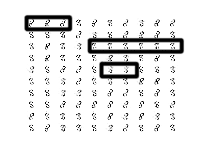
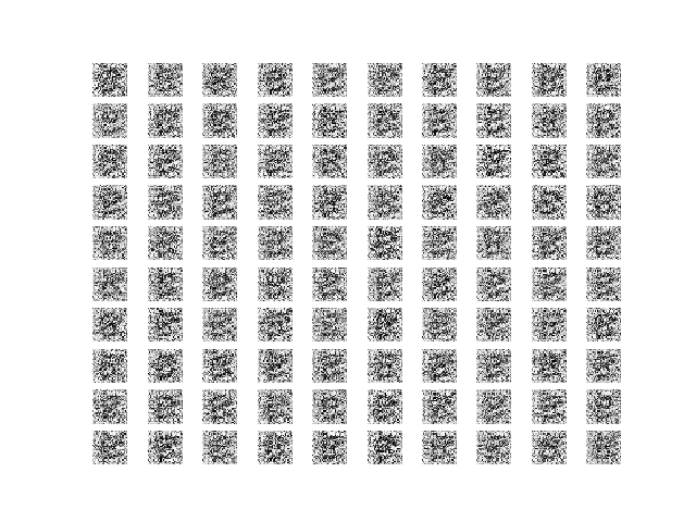
Sample of 100 Generated Images of a Handwritten Number 8 at Epoch 315 From a GAN That Has Suffered Mode Collapse.
A mode collapse is less common during training given the findings from the DCGAN model architecture and training configuration.
In summary, you can identify a mode collapse as follows:
- The loss for the generator, and probably the discriminator, is expected to oscillate over time.
- The generator model is expected to generate identical output images from different points in the latent space.
How To Identify Convergence Failure in a Generative Adversarial Network
Perhaps the most common failure when training a GAN is a failure to converge.
Typically, a neural network fails to converge when the model loss does not settle down during the training process. In the case of a GAN, a failure to converge refers to not finding an equilibrium between the discriminator and the generator.
The likely way that you will identify this type of failure is that the loss for the discriminator has gone to zero or close to zero. In some cases, the loss of the generator may also rise and continue to rise over the same period.
This type of loss is most commonly caused by the generator outputting garbage images that the discriminator can easily identify.
This type of failure might happen at the beginning of the run and continue throughout training, at which point you should halt the training process. For some unstable GANs, it is possible for the GAN to fall into this failure mode for a number of batch updates, or even a number of epochs, and then recover.
There are many ways to impair our stable GAN to achieve a convergence failure, such as changing one or both models to have insufficient capacity, changing the Adam optimization algorithm to be too aggressive, and using very large or very small kernel sizes in the models.
In this case, we will update the example to combine the real and fake samples when updating the discriminator. This simple change will cause the model to fail to converge.
This change is as simple as using the vstack() NumPy function to combine the real and fake samples and then calling the train_on_batch() function to update the discriminator model. The result is also a single loss and accuracy scores, meaning that the reporting of model performance, must also be updated.
The full code listing with these changes is provided below for completeness.
|
1 2 3 4 5 6 7 8 9 10 11 12 13 14 15 16 17 18 19 20 21 22 23 24 25 26 27 28 29 30 31 32 33 34 35 36 37 38 39 40 41 42 43 44 45 46 47 48 49 50 51 52 53 54 55 56 57 58 59 60 61 62 63 64 65 66 67 68 69 70 71 72 73 74 75 76 77 78 79 80 81 82 83 84 85 86 87 88 89 90 91 92 93 94 95 96 97 98 99 100 101 102 103 104 105 106 107 108 109 110 111 112 113 114 115 116 117 118 119 120 121 122 123 124 125 126 127 128 129 130 131 132 133 134 135 136 137 138 139 140 141 142 143 144 145 146 147 148 149 150 151 152 153 154 155 156 157 158 159 160 161 162 163 164 165 166 167 168 169 170 171 172 173 174 175 176 177 178 179 180 181 182 183 184 185 186 187 188 189 190 191 192 193 194 195 196 197 198 199 200 201 202 203 204 205 206 |
# example of training an unstable gan for generating a handwritten digit from os import makedirs from numpy import expand_dims from numpy import zeros from numpy import ones from numpy import vstack from numpy.random import randn from numpy.random import randint from keras.datasets.mnist import load_data from keras.optimizers import Adam from keras.models import Sequential from keras.layers import Dense from keras.layers import Reshape from keras.layers import Flatten from keras.layers import Conv2D from keras.layers import Conv2DTranspose from keras.layers import LeakyReLU from keras.initializers import RandomNormal from matplotlib import pyplot # define the standalone discriminator model def define_discriminator(in_shape=(28,28,1)): # weight initialization init = RandomNormal(stddev=0.02) # define model model = Sequential() # downsample to 14x14 model.add(Conv2D(64, (4,4), strides=(2,2), padding='same', kernel_initializer=init, input_shape=in_shape)) model.add(LeakyReLU(alpha=0.2)) # downsample to 7x7 model.add(Conv2D(64, (4,4), strides=(2,2), padding='same', kernel_initializer=init)) model.add(LeakyReLU(alpha=0.2)) # classifier model.add(Flatten()) model.add(Dense(1, activation='sigmoid')) # compile model opt = Adam(lr=0.0002, beta_1=0.5) model.compile(loss='binary_crossentropy', optimizer=opt, metrics=['accuracy']) return model # define the standalone generator model def define_generator(latent_dim): # weight initialization init = RandomNormal(stddev=0.02) # define model model = Sequential() # foundation for 7x7 image n_nodes = 128 * 7 * 7 model.add(Dense(n_nodes, kernel_initializer=init, input_dim=latent_dim)) model.add(LeakyReLU(alpha=0.2)) model.add(Reshape((7, 7, 128))) # upsample to 14x14 model.add(Conv2DTranspose(128, (4,4), strides=(2,2), padding='same', kernel_initializer=init)) model.add(LeakyReLU(alpha=0.2)) # upsample to 28x28 model.add(Conv2DTranspose(128, (4,4), strides=(2,2), padding='same', kernel_initializer=init)) model.add(LeakyReLU(alpha=0.2)) # output 28x28x1 model.add(Conv2D(1, (7,7), activation='tanh', padding='same', kernel_initializer=init)) return model # define the combined generator and discriminator model, for updating the generator def define_gan(generator, discriminator): # make weights in the discriminator not trainable discriminator.trainable = False # connect them model = Sequential() # add generator model.add(generator) # add the discriminator model.add(discriminator) # compile model opt = Adam(lr=0.0002, beta_1=0.5) model.compile(loss='binary_crossentropy', optimizer=opt) return model # load mnist images def load_real_samples(): # load dataset (trainX, trainy), (_, _) = load_data() # expand to 3d, e.g. add channels X = expand_dims(trainX, axis=-1) # select all of the examples for a given class selected_ix = trainy == 8 X = X[selected_ix] # convert from ints to floats X = X.astype('float32') # scale from [0,255] to [-1,1] X = (X - 127.5) / 127.5 return X # # select real samples def generate_real_samples(dataset, n_samples): # choose random instances ix = randint(0, dataset.shape[0], n_samples) # select images X = dataset[ix] # generate class labels y = ones((n_samples, 1)) return X, y # generate points in latent space as input for the generator def generate_latent_points(latent_dim, n_samples): # generate points in the latent space x_input = randn(latent_dim * n_samples) # reshape into a batch of inputs for the network x_input = x_input.reshape(n_samples, latent_dim) return x_input # use the generator to generate n fake examples, with class labels def generate_fake_samples(generator, latent_dim, n_samples): # generate points in latent space x_input = generate_latent_points(latent_dim, n_samples) # predict outputs X = generator.predict(x_input) # create class labels y = zeros((n_samples, 1)) return X, y # generate samples and save as a plot and save the model def summarize_performance(step, g_model, latent_dim, n_samples=100): # prepare fake examples X, _ = generate_fake_samples(g_model, latent_dim, n_samples) # scale from [-1,1] to [0,1] X = (X + 1) / 2.0 # plot images for i in range(10 * 10): # define subplot pyplot.subplot(10, 10, 1 + i) # turn off axis pyplot.axis('off') # plot raw pixel data pyplot.imshow(X[i, :, :, 0], cmap='gray_r') # save plot to file pyplot.savefig('results_convergence/generated_plot_%03d.png' % (step+1)) pyplot.close() # save the generator model g_model.save('results_convergence/model_%03d.h5' % (step+1)) # create a line plot of loss for the gan and save to file def plot_history(d_hist, g_hist, a_hist): # plot loss pyplot.subplot(2, 1, 1) pyplot.plot(d_hist, label='dis') pyplot.plot(g_hist, label='gen') pyplot.legend() # plot discriminator accuracy pyplot.subplot(2, 1, 2) pyplot.plot(a_hist, label='acc') pyplot.legend() # save plot to file pyplot.savefig('results_convergence/plot_line_plot_loss.png') pyplot.close() # train the generator and discriminator def train(g_model, d_model, gan_model, dataset, latent_dim, n_epochs=10, n_batch=128): # calculate the number of batches per epoch bat_per_epo = int(dataset.shape[0] / n_batch) # calculate the total iterations based on batch and epoch n_steps = bat_per_epo * n_epochs # calculate the number of samples in half a batch half_batch = int(n_batch / 2) # prepare lists for storing stats each iteration d_hist, g_hist, a_hist = list(), list(), list() # manually enumerate epochs for i in range(n_steps): # get randomly selected 'real' samples X_real, y_real = generate_real_samples(dataset, half_batch) # generate 'fake' examples X_fake, y_fake = generate_fake_samples(g_model, latent_dim, half_batch) # combine into one batch X, y = vstack((X_real, X_fake)), vstack((y_real, y_fake)) # update discriminator model weights d_loss, d_acc = d_model.train_on_batch(X, y) # prepare points in latent space as input for the generator X_gan = generate_latent_points(latent_dim, n_batch) # create inverted labels for the fake samples y_gan = ones((n_batch, 1)) # update the generator via the discriminator's error g_loss = gan_model.train_on_batch(X_gan, y_gan) # summarize loss on this batch print('>%d, d=%.3f, g=%.3f, a=%d' % (i+1, d_loss, g_loss, int(100*d_acc))) # record history d_hist.append(d_loss) g_hist.append(g_loss) a_hist.append(d_acc) # evaluate the model performance every 'epoch' if (i+1) % bat_per_epo == 0: summarize_performance(i, g_model, latent_dim) plot_history(d_hist, g_hist, a_hist) # make folder for results makedirs('results_convergence', exist_ok=True) # size of the latent space latent_dim = 50 # create the discriminator discriminator = define_discriminator() # create the generator generator = define_generator(latent_dim) # create the gan gan_model = define_gan(generator, discriminator) # load image data dataset = load_real_samples() print(dataset.shape) # train model train(generator, discriminator, gan_model, dataset, latent_dim) |
Running the example reports loss and accuracy for each model update.
A clear sign of this type of failure is the rapid drop of the discriminator loss towards zero, where it remains.
This is what we see in this case.
|
1 2 3 4 5 6 7 8 9 10 11 12 13 14 15 16 |
>1, d=0.514, g=0.969, a=80 >2, d=0.475, g=0.395, a=74 >3, d=0.452, g=0.223, a=69 >4, d=0.302, g=0.220, a=85 >5, d=0.177, g=0.195, a=100 >6, d=0.122, g=0.200, a=100 >7, d=0.088, g=0.179, a=100 >8, d=0.075, g=0.159, a=100 >9, d=0.071, g=0.167, a=100 >10, d=0.102, g=0.127, a=100 ... >446, d=0.000, g=0.001, a=100 >447, d=0.000, g=0.001, a=100 >448, d=0.000, g=0.001, a=100 >449, d=0.000, g=0.001, a=100 >450, d=0.000, g=0.001, a=100 |
Line plots of learning curves and classification accuracy are created.
The top subplot shows the loss for the discriminator (blue) and generator (orange) and clearly shows the drop of both values down towards zero over the first 20 to 30 iterations, where it remains for the rest of the run.
The bottom subplot shows the discriminator classification accuracy sitting on 100% for the same period, meaning the model is perfect at identifying real and fake images. The expectation is that there is something about fake images that makes them very easy for the discriminator to identify.
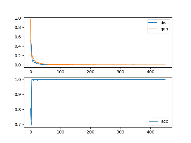
Line Plots of Loss and Accuracy for a Generative Adversarial Network With a Convergence Failure
Finally, reviewing samples of generated images makes it clear why the discriminator is so successful.
Samples of images generated at each epoch are all very low quality, showing static, perhaps with a faint figure eight in the background.
Sample of 100 Generated Images of a Handwritten Number 8 at Epoch 450 From a GAN That Has a Convergence Failure via Combined Updates to the Discriminator.
It is useful to see another example of this type of failure.
In this case, the configuration of the Adam optimization algorithm can be modified to use the defaults, which in turn makes the updates to the models aggressive and causes a failure for the training process to find a point of equilibrium between training the two models.
For example, the discriminator can be compiled as follows:
|
1 2 3 |
... # compile model model.compile(loss='binary_crossentropy', optimizer='adam', metrics=['accuracy']) |
And the composite GAN model can be compiled as follows:
|
1 2 3 |
... # compile model model.compile(loss='binary_crossentropy', optimizer='adam') |
The full code listing is provided below for completeness.
|
1 2 3 4 5 6 7 8 9 10 11 12 13 14 15 16 17 18 19 20 21 22 23 24 25 26 27 28 29 30 31 32 33 34 35 36 37 38 39 40 41 42 43 44 45 46 47 48 49 50 51 52 53 54 55 56 57 58 59 60 61 62 63 64 65 66 67 68 69 70 71 72 73 74 75 76 77 78 79 80 81 82 83 84 85 86 87 88 89 90 91 92 93 94 95 96 97 98 99 100 101 102 103 104 105 106 107 108 109 110 111 112 113 114 115 116 117 118 119 120 121 122 123 124 125 126 127 128 129 130 131 132 133 134 135 136 137 138 139 140 141 142 143 144 145 146 147 148 149 150 151 152 153 154 155 156 157 158 159 160 161 162 163 164 165 166 167 168 169 170 171 172 173 174 175 176 177 178 179 180 181 182 183 184 185 186 187 188 189 190 191 192 193 194 195 196 197 198 199 200 201 202 203 204 205 206 207 |
# example of training an unstable gan for generating a handwritten digit from os import makedirs from numpy import expand_dims from numpy import zeros from numpy import ones from numpy.random import randn from numpy.random import randint from keras.datasets.mnist import load_data from keras.models import Sequential from keras.layers import Dense from keras.layers import Reshape from keras.layers import Flatten from keras.layers import Conv2D from keras.layers import Conv2DTranspose from keras.layers import LeakyReLU from keras.initializers import RandomNormal from matplotlib import pyplot # define the standalone discriminator model def define_discriminator(in_shape=(28,28,1)): # weight initialization init = RandomNormal(stddev=0.02) # define model model = Sequential() # downsample to 14x14 model.add(Conv2D(64, (4,4), strides=(2,2), padding='same', kernel_initializer=init, input_shape=in_shape)) model.add(LeakyReLU(alpha=0.2)) # downsample to 7x7 model.add(Conv2D(64, (4,4), strides=(2,2), padding='same', kernel_initializer=init)) model.add(LeakyReLU(alpha=0.2)) # classifier model.add(Flatten()) model.add(Dense(1, activation='sigmoid')) # compile model model.compile(loss='binary_crossentropy', optimizer='adam', metrics=['accuracy']) return model # define the standalone generator model def define_generator(latent_dim): # weight initialization init = RandomNormal(stddev=0.02) # define model model = Sequential() # foundation for 7x7 image n_nodes = 128 * 7 * 7 model.add(Dense(n_nodes, kernel_initializer=init, input_dim=latent_dim)) model.add(LeakyReLU(alpha=0.2)) model.add(Reshape((7, 7, 128))) # upsample to 14x14 model.add(Conv2DTranspose(128, (4,4), strides=(2,2), padding='same', kernel_initializer=init)) model.add(LeakyReLU(alpha=0.2)) # upsample to 28x28 model.add(Conv2DTranspose(128, (4,4), strides=(2,2), padding='same', kernel_initializer=init)) model.add(LeakyReLU(alpha=0.2)) # output 28x28x1 model.add(Conv2D(1, (7,7), activation='tanh', padding='same', kernel_initializer=init)) return model # define the combined generator and discriminator model, for updating the generator def define_gan(generator, discriminator): # make weights in the discriminator not trainable discriminator.trainable = False # connect them model = Sequential() # add generator model.add(generator) # add the discriminator model.add(discriminator) # compile model model.compile(loss='binary_crossentropy', optimizer='adam') return model # load mnist images def load_real_samples(): # load dataset (trainX, trainy), (_, _) = load_data() # expand to 3d, e.g. add channels X = expand_dims(trainX, axis=-1) # select all of the examples for a given class selected_ix = trainy == 8 X = X[selected_ix] # convert from ints to floats X = X.astype('float32') # scale from [0,255] to [-1,1] X = (X - 127.5) / 127.5 return X # select real samples def generate_real_samples(dataset, n_samples): # choose random instances ix = randint(0, dataset.shape[0], n_samples) # select images X = dataset[ix] # generate class labels y = ones((n_samples, 1)) return X, y # generate points in latent space as input for the generator def generate_latent_points(latent_dim, n_samples): # generate points in the latent space x_input = randn(latent_dim * n_samples) # reshape into a batch of inputs for the network x_input = x_input.reshape(n_samples, latent_dim) return x_input # use the generator to generate n fake examples, with class labels def generate_fake_samples(generator, latent_dim, n_samples): # generate points in latent space x_input = generate_latent_points(latent_dim, n_samples) # predict outputs X = generator.predict(x_input) # create class labels y = zeros((n_samples, 1)) return X, y # generate samples and save as a plot and save the model def summarize_performance(step, g_model, latent_dim, n_samples=100): # prepare fake examples X, _ = generate_fake_samples(g_model, latent_dim, n_samples) # scale from [-1,1] to [0,1] X = (X + 1) / 2.0 # plot images for i in range(10 * 10): # define subplot pyplot.subplot(10, 10, 1 + i) # turn off axis pyplot.axis('off') # plot raw pixel data pyplot.imshow(X[i, :, :, 0], cmap='gray_r') # save plot to file pyplot.savefig('results_opt/generated_plot_%03d.png' % (step+1)) pyplot.close() # save the generator model g_model.save('results_opt/model_%03d.h5' % (step+1)) # create a line plot of loss for the gan and save to file def plot_history(d1_hist, d2_hist, g_hist, a1_hist, a2_hist): # plot loss pyplot.subplot(2, 1, 1) pyplot.plot(d1_hist, label='d-real') pyplot.plot(d2_hist, label='d-fake') pyplot.plot(g_hist, label='gen') pyplot.legend() # plot discriminator accuracy pyplot.subplot(2, 1, 2) pyplot.plot(a1_hist, label='acc-real') pyplot.plot(a2_hist, label='acc-fake') pyplot.legend() # save plot to file pyplot.savefig('results_opt/plot_line_plot_loss.png') pyplot.close() # train the generator and discriminator def train(g_model, d_model, gan_model, dataset, latent_dim, n_epochs=10, n_batch=128): # calculate the number of batches per epoch bat_per_epo = int(dataset.shape[0] / n_batch) # calculate the total iterations based on batch and epoch n_steps = bat_per_epo * n_epochs # calculate the number of samples in half a batch half_batch = int(n_batch / 2) # prepare lists for storing stats each iteration d1_hist, d2_hist, g_hist, a1_hist, a2_hist = list(), list(), list(), list(), list() # manually enumerate epochs for i in range(n_steps): # get randomly selected 'real' samples X_real, y_real = generate_real_samples(dataset, half_batch) # update discriminator model weights d_loss1, d_acc1 = d_model.train_on_batch(X_real, y_real) # generate 'fake' examples X_fake, y_fake = generate_fake_samples(g_model, latent_dim, half_batch) # update discriminator model weights d_loss2, d_acc2 = d_model.train_on_batch(X_fake, y_fake) # prepare points in latent space as input for the generator X_gan = generate_latent_points(latent_dim, n_batch) # create inverted labels for the fake samples y_gan = ones((n_batch, 1)) # update the generator via the discriminator's error g_loss = gan_model.train_on_batch(X_gan, y_gan) # summarize loss on this batch print('>%d, d1=%.3f, d2=%.3f g=%.3f, a1=%d, a2=%d' % (i+1, d_loss1, d_loss2, g_loss, int(100*d_acc1), int(100*d_acc2))) # record history d1_hist.append(d_loss1) d2_hist.append(d_loss2) g_hist.append(g_loss) a1_hist.append(d_acc1) a2_hist.append(d_acc2) # evaluate the model performance every 'epoch' if (i+1) % bat_per_epo == 0: summarize_performance(i, g_model, latent_dim) plot_history(d1_hist, d2_hist, g_hist, a1_hist, a2_hist) # make folder for results makedirs('results_opt', exist_ok=True) # size of the latent space latent_dim = 50 # create the discriminator discriminator = define_discriminator() # create the generator generator = define_generator(latent_dim) # create the gan gan_model = define_gan(generator, discriminator) # load image data dataset = load_real_samples() print(dataset.shape) # train model train(generator, discriminator, gan_model, dataset, latent_dim) |
Running the example reports the loss and accuracy for each step during training, as before.
As we expected, the loss for the discriminator rapidly falls to a value close to zero, where it remains, and classification accuracy for the discriminator on real and fake examples remains at 100%.
|
1 2 3 4 5 6 7 8 9 10 11 |
>1, d1=0.728, d2=0.902 g=0.763, a1=54, a2=12 >2, d1=0.001, d2=4.509 g=0.033, a1=100, a2=0 >3, d1=0.000, d2=0.486 g=0.542, a1=100, a2=76 >4, d1=0.000, d2=0.446 g=0.733, a1=100, a2=82 >5, d1=0.002, d2=0.855 g=0.649, a1=100, a2=46 ... >446, d1=0.000, d2=0.000 g=10.410, a1=100, a2=100 >447, d1=0.000, d2=0.000 g=10.414, a1=100, a2=100 >448, d1=0.000, d2=0.000 g=10.419, a1=100, a2=100 >449, d1=0.000, d2=0.000 g=10.424, a1=100, a2=100 >450, d1=0.000, d2=0.000 g=10.427, a1=100, a2=100 |
A plot of the learning curves and accuracy from training the model with this single change is created.
The plot shows that this change causes the loss for the discriminator to crash down to a value close to zero and remain there. An important difference for this case is that the loss for the generator rises quickly and continues to rise for the duration of training.
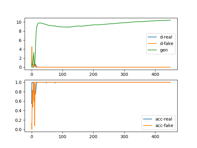
Line Plots of Loss and Accuracy for a Generative Adversarial Network With a Convergence Failure Due To Aggressive Optimization
We can review the properties of a convergence failure as follows:
- The loss for the discriminator is expected to rapidly decrease to a value close to zero where it remains during training.
- The loss for the generator is expected to either decrease to zero or continually decrease during training.
- The generator is expected to produce extremely low-quality images that are easily identified as fake by the discriminator.
Further Reading
This section provides more resources on the topic if you are looking to go deeper.
Papers
- Generative Adversarial Networks, 2014.
- Tutorial: Generative Adversarial Networks, NIPS, 2016.
- Unsupervised Representation Learning with Deep Convolutional Generative Adversarial Networks, 2015.
Articles
Summary
In this tutorial, you discovered how to identify stable and unstable GAN training by reviewing examples of generated images and plots of metrics recorded during training.
Specifically, you learned:
- How to identify a stable GAN training process from the generator and discriminator loss over time.
- How to identify a mode collapse by reviewing both learning curves and generated images.
- How to identify a convergence failure by reviewing learning curves of generator and discriminator loss over time.
Do you have any questions?
Ask your questions in the comments below and I will do my best to answer.
Develop Generative Adversarial Networks Today!
Develop Your GAN Models in Minutes
...with just a few lines of python codeDiscover how in my new Ebook:
Generative Adversarial Networks with Python
It provides self-study tutorials and end-to-end projects on:
DCGAN, conditional GANs, image translation, Pix2Pix, CycleGAN
and much more...


 From Scratch with Keras")

Hello Jason,great article again.
There is my two little questions:
1.In the chapter about Convergence Failure,the first way to mess things up that you mentioned is vstacking the real and false examples.
Its quite out of my mind how come training difference types of sample will causes such failure,especailly after I followed the other post [https://machinelearningmastery.com/how-to-develop-a-generative-adversarial-network-for-an-mnist-handwritten-digits-from-scratch-in-keras/].
In the post linked above you demonstrated vstacking and the results went well.(so as I tried)
2.Maybe the same question with the first one(also happened during trying the post linked above).But a curious things happened when I tried add BatchNormalization layers to the original code of yours,that Convergence Failure happened.
How come harmless-seemed BatchNormalization causes such failure?
Thank you for reading this long questions.Looking forward to hear your reply.
Best Reguards.
By the by,I tried your work in kaggle.link is : https://www.kaggle.com/jinyongnan/the-basic-2dgans
Version 3 is the one with BatchNormalization,Version 4 is the one without.
Good questions.
It is often better to not stack real/fake images during training. Perhaps try both ways and see what works best for your specific problem.
The models are very sensitive and small changes can cause a failure. Test changes carefully, and cause and effect (the why) is challenging to determine.
Do you know any papers or other sources that analyze in more depth why it is better not to stack real and fake images during training? That is very unintuitive to me as well, and I’d like to learn more about why this is the case.
Not really, like most of the GAN heuristics it is empirical/tacit knowledge.
This might have something:
https://github.com/soumith/ganhacks
It seems to be related to batch normalization. My initial trial seems to suggest that if you use batch normalization, and you train the discriminator with a mixed real/fake batch, it may run into problem. If you train with batch containing only real follow by only fake, you may still run into problem, but at much later epochs. Also, if you do run into problem (i.e. loss goes to 0 or inf), you can stop training, and load the parameters from last saved point when the model was still ok. When you continue training, you may not fall into the same quagmire.
Great observation!
Sorry I only find here to ask questions, I’m very appreciate of your article, I have 2 questions:
1. during training of generator and discriminator, should we set optimizer decay learning rate? I have read some code and found they didn’t set it but it is a comman setting during many other deep learning task.
2. I use pytorch to train my GAN model, during training of generator, should we use model.eval() to freeze discriminator?also the same treatment should we take for generator when training for discriminator?
Forgive my poor English, I’m looking forward for your replay!
Hi John…You may want to start here:
https://machinelearningmastery.com/start-here/#gans
If you are interested I tested your stable architecture with a few changes:
(Dis is discriminator, gen is generator)
Averagepooling in dis, upsampling in gen, stride = 1×1:
https://drive.google.com/file/d/1K8CFI1X3CORXBvXKOUaCAI8L0aKobLpa/view?usp=sharing
(I didn’t detect changes in the quality of the gen output after training on MNIST dataset, but on comclicated data it gives better results instead stride = 2×2)
++ Filters sizes = 3×3:
https://drive.google.com/file/d/1nuIKvTleXNBtDdOgL4UQ46YA7I-RJOk9/view?usp=sharing
(A little bit worse image generation but everyone recommends using odd filter size)
++ FIlters numer 32-64 in dis and 64-32 in gen instead 64-64 in dis and 128-128 in gen:
https://drive.google.com/file/d/1QwaUbTw9Fs3hGpYhLE7zTJyJCnmRBKyk/view?usp=sharing
(Same generated imgs after training, but using mirror-like generator and discriminator maximizes network training stability. You’ll not notice this on simple datasets like MNIST, but i have seen training crash on complicated 3D data just because im using non mirrored GAN)
++ Dis learning rate x2:
https://drive.google.com/file/d/1IkUuKZNlBCiNJqKkAWHtDvQyw-Tvomlg/view?usp=sharing
(I saw that it is used sometimes but dont know why. I have tested x3, but more smooth loss and training accuracy on x2)
Comprasion (before/after):
iteration 45:
before – https://drive.google.com/open?id=1uaiSp_OCIlcV79wYfybDMJR3g3xR7O4C
after – https://drive.google.com/open?id=1Mu6BInIVnC17jigiTh4L1aOqAnieeitv
iteration 450:
before – https://drive.google.com/open?id=1Bspoo7BwuzyaA7CCYVig1d2qfTyNrHSa
after – https://drive.google.com/open?id=1vwmtinHEGDfkrB-TTU8-XhtVrb30jEPK
sorry for my poor English
Not at all, we want results, not great english around here 🙂
Thanks for sharing!
Hello,
First of all, thank you for the article!
I have a question. After training my model for 500 epochs, the acc_real and acc_fake remain 0. There is no change during training and generated images indicate that the model fails to converge. The loss for discriminator and generator oscillates but most remains at 0. Can you explain this and how to solve it?
Generally, GAN models do not converge. I explain more here:
https://machinelearningmastery.com/faq/single-faq/why-is-my-gan-not-converging
Thank you for the suggestion.
I fixed the problem by removing label smoothing. The loss and acc are fluctuating as expected. However, when I looked at the generated images, the images look like they are improving and then back to noisy images again and repeat that many times during training. Can you help me figure out why the situation happened?
Well done.
Yes, you must save models frequently during training, then post-hoc evaluate them by the images they generate in order to choose a final model.
That is really great article. Thanks, Jason
Thanks, I’m happy it helped!
Hi Jason. Thanks for the great article !
I’m training a pix2pix model, my discriminator losses on both real and fake sample vary around 0.3 after few iterations, while generator loss go down. Do you know what this indicates ?
If you have time, please take a look at my graphs.
https://drive.google.com/file/d/16NSq5FdKRyIm3oxrVXCXL1-yU9LefGRS/view?usp=sharing
No.
Perhaps try some of the countermeasures here:
https://machinelearningmastery.com/how-to-code-generative-adversarial-network-hacks/
Hi Jason, I modified your pix2pix implementation, so most of the hacks are implemented already. I use mae and log loss for generator. I might be wrong but It’s seem that the remaining differences (20×20) is too small compare to input size (512,512). Therefor the loss very really small and discriminator and generator loss can’t go any lower. Do you have any suggestion to make the networks learn low level features better ?
Nice work!
Not offhand, explore ideas with controlled experiments.
Hi Jason!
great work as always! I have a little problem with the GAN I am currently training and would love to hear your opinion on this.
So I have input data consisting of 1008 features where each feature gets 0/1 and portrays whether or not someone ist at home during a 10min interval.
My goal is to make the GAN create those kind of activity profiles. However, the problem I face is that my GAN currently creates profiles where the shares of single timestep activity durations (a person is outside for 10min and then at home again, or the other way: is at home for 10min and then goes outside again) are way higher than in the real data. The shares of other activity duration (20min, 30min, 40min …) are very close to the real data! This really confuses me.. The GAN model creates realistic data besides for having too many of these little errors.
What do you think about this? What could solve this issue?
Best regards,
Abdullah
You perhaps should use a generative model that allow you to impose constraints to ensure generated data is plausible.
Perhaps look into probabilistic graphical models.
How to Reduce Noise in Generated image,
Is dropout and Adam possible to use in GAN
Some ideas here:
https://machinelearningmastery.com/how-to-code-generative-adversarial-network-hacks/
Hi Jason,
Thanks for the very nice article. I have two questions:
Question 1: I have trained a GAN and obtained the log loss shown in the image in below URL. How do I interpret this? More specifically, what does it tell about the following:
https://drive.google.com/file/d/1F7U8CJoSFEC81B8FyOXwu9LhikUD3-vi/view?usp=sharing
(i) Generator convergence
(ii) Discriminator performance
(iii) Which iteration the training should be stopped?
(iv) The generator model produced at which iteration should be used to generate plausible data?
Question 2: After training a GAN, why we are not taking the generator model produce at the last training iteration to generate plausible data? Isn’t the GAN convergence always improve as the training iterations increase?
GANs don’t converge:
https://machinelearningmastery.com/faq/single-faq/why-is-my-gan-not-converging
No. You save models throughput the run, test each and pick one that produces results that you like.
Hi Jason,
Thanks for the answer. Can you please have a look at the 1st question in my post as well?
From the plot, the training process might be stable.
Thanks for the great article! It is very useful.
Two interesting questions remain to be dark matter for me.
1. How does latent space size affect a model convergence?
2. What are recomendations for model capacities in general? (total number of trainable parameters) and to not to overestimate/underestimate required capacity for a given task.
Would you share your intuition on that.
Thanks again for the great article.
GANs don’t converge:
https://machinelearningmastery.com/faq/single-faq/why-is-my-gan-not-converging
We don’t have good theories re model size vs capability. The best we can do is controlled experiments.
Hello professor!
Fabulous article as always.
It helped me a lot to figure out how my model is doing.
I have a question for you! I realized that you have used random normal initialized with std 0.02, and I wonder what was the idea behind it.
I just encountered Nan in my gradient, and I suspect that the wrong initializer might be the one that caused it. (it was glorot uniform, which was the default initializer)
I have gradient clipping enabled so not sure where the gradient could overshoot.
Do you have any suggestions in this case?
Thank you!
Sincerely
I’m not a professor.
You can see the reason why here:
https://machinelearningmastery.com/how-to-code-generative-adversarial-network-hacks/
Hello Jason,
Thank you so much for you very intuitive and instructive lessons !
Thanks to you, I’ve implemented an auxiliary classifier GAN to produce some medical images.
The architecture is more or less the same as here :
https://drive.google.com/file/d/1vFcfb9JuBovlfAN4ajBdcTtmMbxOn35z/view?usp=sharing
found in [1].
After some training, I’ve got always the learning curves as follows :
https://drive.google.com/file/d/1AbTV41MizaJJaxYEOJSkV2wgKI9G4W9S/view?usp=sharing
Your tips are very instructive and after implementation and few modifications in the architecture the curves looks like this :
https://drive.google.com/file/d/1yoH9voIv6xyFKHogg_AnnGMjuEyBm3hu/view?usp=sharing
Not perfect but still the best training until now by observing the curves and the output images.
However, for each class, the generator produce each time variations of the same image or noisy images.
Do you have any recommandations ?
Thank you again for your lessons !
[1] Madani A. et al., Deep echocardiography: data-efficient supervised and semi-supervised deep learning towards automated diagnosis of cardiac desease, In: NPJ Digital Medicine vol 1. 2018.
Well done!
Sorry, I don’t open attachments.
Perhaps try adjusting the model or training parameters? Experiment.
hello
would you please share your code
Hello,
I’ve copy-pasted this code but the results are completely different (aka not converging). Would it be possible to make the code deterministic?
Thanks
GANs do not converge:
https://machinelearningmastery.com/faq/single-faq/why-is-my-gan-not-converging
No, the stochastic nature of the learning algorithm is a feature, not a bug.
Thanks for the reply but I do not agree. Despite I understand the stochastic nature of GAN, non-determinism in testing is never a feature, especially when it prevents an article to be reproduced: a seed shall be provided in order to make it deterministic and reproducible.
Thanks for sharing your opinion.
Hi, Jason,
Thanks for your great post.
I have question, it’s about vstacking the real and fake images to train the discriminator.
I have tried the code, and got the same result as yours. What confused me is the loss of G and acc of D. As we observed, the acc of D is near 100%, which means D can identify almost every image correctly(partially due to the poor quality of the generated fake image, it seems they are easy to identify). However, why the loss of G is so low, to my intuitive, the generated fake images are easy to be identified as fake, the loss of G should be very high. Can you tell me where I am wrong, thanks.
You’re welcome!
Accuracy might be a bad metric to monitor during training.
Also, loss does not give ideas about the skill of the GAN, e.g. GAN’s don’t converge, they are unstable by definition:
https://machinelearningmastery.com/faq/single-faq/why-is-my-gan-not-converging
Hi Jason,
Great Tutorial!! I ran into a problem with my gan where the losses were in range and stabilized but my discriminator accuracy does not seem to go above 50 for both real and fake images in spite of using a pre trained model. What does the error possibly be?
Thanks.
Ignore accuracy, it’s not a reliable metric. Focus on loss.
And all the output images also just seem to be plain gray images.
Perhaps try changing the architecture of the model or the hyperparameters of the learning algorithm:
https://machinelearningmastery.com/how-to-code-generative-adversarial-network-hacks/
Thanks for the article
my generator loss is showing huge variation from -500 t +500 but discrimnator loss is almost constant varying from 0.3 to 0.6.Please help me out i m really stuck
Perhaps focus on the generated images and whether that are good or not.
Hi Jason,
I am an MSc Candidate in A.I.
I am employing cGan model in an effort to generate reliable COVID-19 CXR and, I found your post useful.
Thank you for your helpful explanation you provide.
I really appreciate your effort and your passion doing this.
Very Best,
Stefanos
You’re welcome!
Very practical and useful guide!
looking forward for StyleGAN implementation.
just a little note: maybe you meant “increase” in the following sentence of the last section:
The loss for the generator is expected to either decrease to zero or continually decrease during training.
Thanks!
Thanks!
Why would we expect loss increase?
if I understood it correctly, in the paragraph below, you present the properties of convergence failure during GANs training. Among these properties we found (as you mentionned): The loss for the generator is expected to either decrease to zero or continually “increase” during training.
Correct me if I am wrong please.
Thanks!
—————————————————————————————
We can review the properties of a convergence failure as follows:
-)The loss for the discriminator is expected to rapidly decrease to a value close to zero where it remains during training.
-)The loss for the generator is expected to either decrease to zero or continually decrease during training.
-)The generator is expected to produce extremely low-quality images that are easily identified as fake by the discriminator.
As heuristics, these are a good start for a DCGAN.
Very Nice, thanks!
You’re welcome!
Hey Jason, thanks for such a great article.
Here are some problems I’ve faced and doubts I have:
1:
I’ve copied the code exactly as in the article for the stable GAN.
But my plots do not seem to match at all, my plots from your stable GAN code seem to match the plots of the code for convergence failure.
Generated images are almost garbage, as expected.
2:
I found the terminology used for ‘epoch’ in this article very confusing.
An epoch is when the model is trained on the entire dataset once, right?
This definition of epoch complies with the one in the code.
However, when you mentioned epoch in the article, you refer to every step trained on a batch.
Could you please clarify on these?
Thanks.
You might need to try training a GAN a few times until you get a useful model/reliable training process.
Agreed!!! Epoch stops making sense with GANs. It’s really iterations of a single batch.
The GAN used in this post is basically DCGAN? Because it uses convolutional layers?
Sure, but we concepts are general to most GANs.
hi
thanks for your article
I have a question
I am working on 3D image and i use adam optimizer.I set learning rate=1e-04 for Dis and 1.1e-05 for Gen
the loss of my Disc goes around 0.4-0.6 but the loss of Gen rise
would you please help me?
Perhaps try using SGD directly and explore different learning rates.
Hi Jason, thanks for the great tutorial! What would you do if you found the d-real loss to be at a good range (around 0.5) but both d-fake and g are going to zero? This has made me quite unsure about if the generator or the discriminator is too weak/too strong, because d-fake going to zero would suggest that the discriminator is too strong, clearly identifying fake images, but g going to zero would suggest that the generator is too strong… Any idea what I should change in this case? Thanks a lot!
Solved this by removing BatchNormalization layers!
Nice!
You’re welcome.
There’s no good loss values for GANs, instead there are dynamics for the two models to focus on/watch. Zero loss is probably a bad sign – meaning one model is dominating.
Hi Jason, you say: “A stable GAN will have a discriminator loss around 0.5, typically between 0.5 and maybe as high as 0.7 or 0.8. The generator loss is typically higher and may hover around 1.0, 1.5, 2.0, or even higher.”
Is there anything you can direct me to that explains a bit more in detail why these values are ideal? I’m trying to understand the math behind binary cross entropy and why these are the most optimal values, is there any paper/article that goes more in depth on that? Thank you.
No, it from experience. We don’t have good theories of GANs.
Hi Jason,
Thanks for a very nice article! I have an additional question. I’m training a Wasserstein GAN myself. As you may know, these don’t have a softmax activation at the end, and correspondingly the ‘discriminator’ is not really a discriminator, but a ‘critic’. This means that I don’t have an accuracy, and my loss is very different.
Do you know if for Wasserstein GANs there are similar ways to identify convergence failure or mode collapse from the loss function (or any other metric I could potentially compute)?
It does not as far as I know. Instead, watch the generated images every n epochs to get an idea of how well the model is going.
Hello Jason, it was a wonderful tutorial! I had a question. I saw that my gan was mode collapsed . How can I fix this? How can we fix a gan that is going through mode collapse?
The discriminator real loss was around 0.6, discriminator fake loss was around 0.7, and the generator loss was around 0.55 the whole time (these values changes sometimes, but most of time these values were present). How can I fix a gan going through Mode Collapse?
Remember to focus on the generated images, not the loss values.
Thanks!
Perhaps try some of these methods:
https://machinelearningmastery.com/how-to-code-generative-adversarial-network-hacks/
I have adapted quite of your model and from the paper you have implemented and fitted on blurr data of motion and defocused after 100 epochs the pics which i got as an output where almost accurate but too much pixelated ..i have not created checkpoints and have just the lats 100th model ..so could you give me a way so i could train once again several time from the 100th model…..and any other suggestion to have in model to increase the clarity of pic
Yes, these tips will give you ideas of things to try:
https://machinelearningmastery.com/how-to-code-generative-adversarial-network-hacks/
Hello Jason, great article!
1. I didn’t understand why in the first example of failure to converge both losses went to 0.
Isn’t is a zero-sum game? Shouldn’t the GANloss go up as the discriminator goes to 0?
2. What should I do when the second described problem, failure to converge, occur?
Thanks!
The losses can’t go to zero, one model will have zero loss, e.g. the discriminator and the other will be close to zero but not zero.
GANs’ don’t converge.
These tips will help improve GAN performance:
https://machinelearningmastery.com/how-to-code-generative-adversarial-network-hacks/
Hi Jason,
Great article!
I created very similar version of GAN like yours in pytorch.
I used it to predict temperature maps, not real RGB or binary images.
for some reason my Discriminator in the beginning stuck on the same loss 0.693 from the first iteration, and does not go up or down, do you have any idea what to do in that situation?
also can I changes the last layer in the Generator to be ReLU and not Tanh, because my maps are normalized to be between 0-1.
Thanks.
Well done.
Perhaps some of the suggestions here will help:
https://machinelearningmastery.com/how-to-code-generative-adversarial-network-hacks/
Hi Jason,
Good article!
I have built a GAN for text line image denoising. However, during training, I noticed that the PSNR evaluated on avalidation data every 4 epochs is not stable as following :
epoch psnr
0 11.23549198
1 11.06054743
2 13.47806442
3 15.43679847
4 16.32856713
5 16.41565544
8 5.565504805
12 17.37565203
16 17.53865563
Especially at epoch 8, is that behaviour is normal??
Thank you.
I don’t think there is a “normal” when it comes to training GANs.
Perhaps focus on the capability of the model instead of loss – unless you get a mode failure.
Sir, the last layer of the discriminator model and generator model is sigmoid and tanh activations respectively. The range of sigmoid function is [0 to 1] and that of tanh is [-1 to 0]. But the d loss and g loss is going beyond these ranges both in stable GAN and unstable GAN.
Please reply the needful as soon as possible.
Reviewing the loss of a GAN is not helpful in determining whether it has a good fit, e.g. GAN’s don’t converge:
https://machinelearningmastery.com/faq/single-faq/why-is-my-gan-not-converging
hi ii have tried this code and after some epochs trained this error is occurred
TypeError: unsupported operand type(s) for *: ‘Sequential’ and ‘int’ at line 3 x_input =rand(latent *)
def generate_latent_points(latent_dim, n_samples):
# generate points in the latent space
x_input = randn(latent_dim * n_samples)
# reshape into a batch of inputs for the network
x_input = x_input.reshape(n_samples, latent_dim)
print(x_input)
return x_input
sorry accidentally sequential data pass through summurization function
No problem.
Sorry to hear that, this may help:
https://machinelearningmastery.com/faq/single-faq/why-does-the-code-in-the-tutorial-not-work-for-me
Hi,
I managed to fix gan failure mode by removing Batch Norm layer in the discriminator in my Semi Supervised GAN. I am now noticing though that the generator is not able to fool the discriminator at all so the discriminator accuracy is 100%
You can ignore accuracy.
Focus on the generated images.
Brilliant article, thank you for posting it.
I have a question on the relationship between the size of a dataset and whether this can impact the stability of the GAN.
I.e. if you had a small dataset would this take longer to reach equilibrium in theory, is there a cut off to minimum size of the dataset where a GAN will just never to able to reach equilibrium?
Thanks!
I’m sure there is, I don’t think it’s an easy relationship to describe at this stage.
Excellent as always, thank you for posting this!
I get discriminator losses that are close to zero (e.g. 0.032) and at the same time I get generator loss somewhere around 3.988. This happens around epoch 20 and goes on until epoch 40 (that is as far as I have tried training the model for). Is that a sign that I should give up training? Looking at the resulting images is rather inconclusive, as I am trying this on spectrograms and their appearance does not give me a clue as to how well the GAN is doing. It might improve after many epochs or maybe not. I wouldn’t like to wait in vain, though.
Also, how can I resume training with this model? How do I load the weights and which model do I load them on?
Image quality is the main way to decide, also it can come good later.
You can save/load images any time, e.g.:
https://machinelearningmastery.com/save-load-keras-deep-learning-models/
Hi,
Can you explain why if a GAN does not converge then both discriminator and generator losses are close to zero? If the discriminator is good at identifying which images are real and which images are fake, then why is it fooled by the generator?
Thanks
Yes, see this:
https://machinelearningmastery.com/faq/single-faq/why-is-my-gan-not-converging
I found the fake images you trained, such as 8, have some artifacts around the number 8. So how to reduce the artifacts in the generated images when we train the GAN?
Probably you can try some of the GAN hacks here: https://machinelearningmastery.com/how-to-code-generative-adversarial-network-hacks/
Hi Jason, thanks for your great article first!
And have you experienced a sudden model failure after like 20 epochs? At beginning everything is fine, and suddenly at a certain epoch, the model totally fail and create garbage pics.
I put generated pics and loss curve pics here:
https://docs.google.com/document/d/1EGNLhIbN2PS91vx93rDG54IPBGgPoova/edit?usp=sharing&ouid=105449882848905790783&rtpof=true&sd=true
That is possible. Hence you need to monitor the loss and stop the training.
Generator weights NAN while training:-
I am using skin cancer datasets (https://challenge.isic-archive.com/data – 2016, melanoma only) for training GAN. After multiple epochs the generator weights become NaN (I think too large for float32).
I have tried with DCGAN (Adam and SGD -> optimiser), bigGAN, custom model made by me.
I have tried adding/removing spectral norm layer, batch norm layer and regularizers but none help me out.
I have also check for null values in my data (not found any).
I my last few experiments i have done ->
# batch size -> 128, dis-lr : 1E-4, gen-lr : 4E-4, no-null till apprx. 1650 epochs
# batch size -> 256, dis-lr : 1E-4, gen-lr : 4E-4, null at epoch 162
# batch size -> 512, dis-lr : 1E-4, gen-lr : 16E-4, null at epoch 1439
with optimiser -> SGD; momentum -> 0.9; target image size 64 x 64 x 3;
What is the real cause behind this ?
I have read various github / stack overflow pages, but still all they did not help me out.
Pages link ->
1. https://stackoverflow.com/questions/33962226/common-causes-of-nans-during-training
2. https://stackoverflow.com/questions/52211665/why-do-i-get-nan-loss-value-in-training-discriminator-and-generator-of-gan
3. https://github.com/eriklindernoren/Keras-GAN/issues/87
4. https://github.com/tensorflow/tensorflow/issues/38416
If your weights are NaN, that’s because of the gradient blow up likely. You may need to tune your optimizer. See this for an example in SGD: https://stackoverflow.com/questions/52000103/weights-of-keras-model-are-nan
Hi Jason,
I am running my model for 3000 epochs, but the discriminator loss went to 0 in the 5th epoch and accuracy also is 100.
Generator loss is close to 1 after 10 epochs.
Using Pix2Pix GAN.
What are your thoughts on it?
Hello Aditi…You may be working on a regression problem and achieve zero prediction errors.
Alternately, you may be working on a classification problem and achieve 100% accuracy.
This is unusual and there are many possible reasons for this, including:
You are evaluating model performance on the training set by accident.
Your hold out dataset (train or validation) is too small or unrepresentative.
You have introduced a bug into your code and it is doing something different from what you expect.
Your prediction problem is easy or trivial and may not require machine learning.
The most common reason is that your hold out dataset is too small or not representative of the broader problem.
This can be addressed by:
Using k-fold cross-validation to estimate model performance instead of a train/test split.
Gather more data.
Use a different split of data for train and test, such as 50/50.
Hello!
Still learning GANs
What does it mean when my discriminator accuracy oscillates between 0 and 1 throughout?
TIA!
Hi Nandini…The following may be of interest to you:
https://neptune.ai/blog/gan-loss-functions
In the pseudocode for a good model, you have latent_size equal to 50. That results in model collapse. You mention that to cause the model collapse to change ‘from 100 to 1’ in latent_size, so I’m assuming the latent_size should be 100 actually, not 50!
Great feedback Alexandras! We appreciate it!
hi
I need a paper or book stating fid metric and is metric
pls I need them to know the enhancement.
Hi Israa…Please rephrase and/or clarify your question so that we may better assist you.
This article is great, thanks.
You are very welcome! We appreciate your feedback and support!