The Cycle Generative Adversarial Network, or CycleGAN, is an approach to training a deep convolutional neural network for image-to-image translation tasks.
Unlike other GAN models for image translation, the CycleGAN does not require a dataset of paired images. For example, if we are interested in translating photographs of oranges to apples, we do not require a training dataset of oranges that have been manually converted to apples. This allows the development of a translation model on problems where training datasets may not exist, such as translating paintings to photographs.
In this tutorial, you will discover how to develop a CycleGAN model to translate photos of horses to zebras, and back again.
After completing this tutorial, you will know:
How to load and prepare the horses to zebras image translation dataset for modeling.
How to train a pair of CycleGAN generator models for translating horses to zebras and zebras to horses.
How to load saved CycleGAN models and use them to translate photographs.
The benefit of the CycleGAN model is that it can be trained without paired examples. That is, it does not require examples of photographs before and after the translation in order to train the model, e.g. photos of the same city landscape during the day and at night. Instead, the model is able to use a collection of photographs from each domain and extract and harness the underlying style of images in the collection in order to perform the translation.
The model architecture is comprised of two generator models: one generator (Generator-A) for generating images for the first domain (Domain-A) and the second generator (Generator-B) for generating images for the second domain (Domain-B).
Generator-A -> Domain-A
Generator-B -> Domain-B
The generator models perform image translation, meaning that the image generation process is conditional on an input image, specifically an image from the other domain. Generator-A takes an image from Domain-B as input and Generator-B takes an image from Domain-A as input.
Domain-B -> Generator-A -> Domain-A
Domain-A -> Generator-B -> Domain-B
Each generator has a corresponding discriminator model. The first discriminator model (Discriminator-A) takes real images from Domain-A and generated images from Generator-A and predicts whether they are real or fake. The second discriminator model (Discriminator-B) takes real images from Domain-B and generated images from Generator-B and predicts whether they are real or fake.
The discriminator and generator models are trained in an adversarial zero-sum process, like normal GAN models. The generators learn to better fool the discriminators and the discriminator learn to better detect fake images. Together, the models find an equilibrium during the training process.
Additionally, the generator models are regularized to not just create new images in the target domain, but instead translate more reconstructed versions of the input images from the source domain. This is achieved by using generated images as input to the corresponding generator model and comparing the output image to the original images. Passing an image through both generators is called a cycle. Together, each pair of generator models are trained to better reproduce the original source image, referred to as cycle consistency.
There is one further element to the architecture, referred to as the identity mapping. This is where a generator is provided with images as input from the target domain and is expected to generate the same image without change. This addition to the architecture is optional, although results in a better matching of the color profile of the input image.
Domain-A -> Generator-A -> Domain-A
Domain-B -> Generator-B -> Domain-B
Now that we are familiar with the model architecture, we can take a closer look at each model in turn and how they can be implemented.
The paper provides a good description of the models and training process, although the official Torch implementation was used as the definitive description for each model and training process and provides the basis for the the model implementations described below.
Want to Develop GANs from Scratch?
Take my free 7-day email crash course now (with sample code).
Click to sign-up and also get a free PDF Ebook version of the course.
How to Prepare the Horses to Zebras Dataset
One of the impressive examples of the CycleGAN in the paper was to transform photographs of horses to zebras, and the reverse, zebras to horses.
The authors of the paper referred to this as the problem of “object transfiguration” and it was also demonstrated on photographs of apples and oranges.
In this tutorial, we will develop a CycleGAN from scratch for image-to-image translation (or object transfiguration) from horses to zebras and the reverse.
We will refer to this dataset as “horses2zebra“. The zip file for this dataset about 111 megabytes and can be downloaded from the CycleGAN webpage:
Download the dataset into your current working directory.
You will see the following directory structure:
1
2
3
4
5
horse2zebra
├── testA
├── testB
├── trainA
└── trainB
The “A” category refers to horse and “B” category refers to zebra, and the dataset is comprised of train and test elements. We will load all photographs and use them as a training dataset.
The photographs are square with the shape 256×256 and have filenames like “n02381460_2.jpg“.
The example below will load all photographs from the train and test folders and create an array of images for category A and another for category B.
Both arrays are then saved to a new file in compressed NumPy array format.
1
2
3
4
5
6
7
8
9
10
11
12
13
14
15
16
17
18
19
20
21
22
23
24
25
26
27
28
29
30
31
32
33
34
35
36
37
# example of preparing the horses and zebra dataset
from os import listdir
from numpy import asarray
from numpy import vstack
from keras.preprocessing.image import img_to_array
from keras.preprocessing.image import load_img
from numpy import savez_compressed
# load all images in a directory into memory
def load_images(path,size=(256,256)):
data_list=list()
# enumerate filenames in directory, assume all are images
forfilename inlistdir(path):
# load and resize the image
pixels=load_img(path+filename,target_size=size)
# convert to numpy array
pixels=img_to_array(pixels)
# store
data_list.append(pixels)
returnasarray(data_list)
# dataset path
path='horse2zebra/'
# load dataset A
dataA1=load_images(path+'trainA/')
dataAB=load_images(path+'testA/')
dataA=vstack((dataA1,dataAB))
print('Loaded dataA: ',dataA.shape)
# load dataset B
dataB1=load_images(path+'trainB/')
dataB2=load_images(path+'testB/')
dataB=vstack((dataB1,dataB2))
print('Loaded dataB: ',dataB.shape)
# save as compressed numpy array
filename='horse2zebra_256.npz'
savez_compressed(filename,dataA,dataB)
print('Saved dataset: ',filename)
Running the example first loads all images into memory, showing that there are 1,187 photos in category A (horses) and 1,474 in category B (zebras).
The arrays are then saved in compressed NumPy format with the filename “horse2zebra_256.npz“. Note: this data file is about 570 megabytes, larger than the raw images as we are storing pixel values as 32-bit floating point values.
1
2
3
Loaded dataA: (1187, 256, 256, 3)
Loaded dataB: (1474, 256, 256, 3)
Saved dataset: horse2zebra_256.npz
We can then load the dataset and plot some of the photos to confirm that we are handling the image data correctly.
The complete example is listed below.
1
2
3
4
5
6
7
8
9
10
11
12
13
14
15
16
17
18
19
# load and plot the prepared dataset
from numpy import load
from matplotlib import pyplot
# load the dataset
data=load('horse2zebra_256.npz')
dataA,dataB=data['arr_0'],data['arr_1']
print('Loaded: ',dataA.shape,dataB.shape)
# plot source images
n_samples=3
foriinrange(n_samples):
pyplot.subplot(2,n_samples,1+i)
pyplot.axis('off')
pyplot.imshow(dataA[i].astype('uint8'))
# plot target image
foriinrange(n_samples):
pyplot.subplot(2,n_samples,1+n_samples+i)
pyplot.axis('off')
pyplot.imshow(dataB[i].astype('uint8'))
pyplot.show()
Running the example first loads the dataset, confirming the number of examples and shape of the color images match our expectations.
1
Loaded: (1187, 256, 256, 3) (1474, 256, 256, 3)
A plot is created showing a row of three images from the horse photo dataset (dataA) and a row of three images from the zebra dataset (dataB).
Plot of Photographs from the Horses2Zeba Dataset
Now that we have prepared the dataset for modeling, we can develop the CycleGAN generator models that can translate photos from one category to the other, and the reverse.
How to Develop a CycleGAN to Translate Horse to Zebra
In this section, we will develop the CycleGAN model for translating photos of horses to zebras and photos of zebras to horses
The same model architecture and configuration described in the paper was used across a range of image-to-image translation tasks. This architecture is both described in the body paper, with additional detail in the appendix of the paper, and a fully working implementation provided as open source implemented for the Torch deep learning framework.
The implementation in this section will use the Keras deep learning framework based directly on the model described in the paper and implemented in the author’s codebase, designed to take and generate color images with the size 256×256 pixels.
The architecture is comprised of four models, two discriminator models, and two generator models.
The discriminator is a deep convolutional neural network that performs image classification. It takes a source image as input and predicts the likelihood of whether the target image is a real or fake image. Two discriminator models are used, one for Domain-A (horses) and one for Domain-B (zebras).
The discriminator design is based on the effective receptive field of the model, which defines the relationship between one output of the model to the number of pixels in the input image. This is called a PatchGAN model and is carefully designed so that each output prediction of the model maps to a 70×70 square or patch of the input image. The benefit of this approach is that the same model can be applied to input images of different sizes, e.g. larger or smaller than 256×256 pixels.
The output of the model depends on the size of the input image but may be one value or a square activation map of values. Each value is a probability for the likelihood that a patch in the input image is real. These values can be averaged to give an overall likelihood or classification score if needed.
A pattern of Convolutional-BatchNorm-LeakyReLU layers is used in the model, which is common to deep convolutional discriminator models. Unlike other models, the CycleGAN discriminator uses InstanceNormalization instead of BatchNormalization. It is a very simple type of normalization and involves standardizing (e.g. scaling to a standard Gaussian) the values on each output feature map, rather than across features in a batch.
An implementation of instance normalization is provided in the keras-contrib project that provides early access to community supplied Keras features.
The keras-contrib library can be installed via pip as follows:
The new InstanceNormalization layer can then be used as follows:
1
2
3
4
5
...
from keras_contrib.layers.normalization.instancenormalization import InstanceNormalization
# define layer
layer=InstanceNormalization(axis=-1)
...
The “axis” argument is set to -1 to ensure that features are normalized per feature map.
The define_discriminator() function below implements the 70×70 PatchGAN discriminator model as per the design of the model in the paper. The model takes a 256×256 sized image as input and outputs a patch of predictions. The model is optimized using least squares loss (L2) implemented as mean squared error, and a weighting it used so that updates to the model have half (0.5) the usual effect. The authors of CycleGAN paper recommend this weighting of model updates to slow down changes to the discriminator, relative to the generator model during training.
The generator model is more complex than the discriminator model.
The generator is an encoder-decoder model architecture. The model takes a source image (e.g. horse photo) and generates a target image (e.g. zebra photo). It does this by first downsampling or encoding the input image down to a bottleneck layer, then interpreting the encoding with a number of ResNet layers that use skip connections, followed by a series of layers that upsample or decode the representation to the size of the output image.
First, we need a function to define the ResNet blocks. These are blocks comprised of two 3×3 CNN layers where the input to the block is concatenated to the output of the block, channel-wise.
This is implemented in the resnet_block() function that creates two Convolution-InstanceNorm blocks with 3×3 filters and 1×1 stride and without a ReLU activation after the second block, matching the official Torch implementation in the build_conv_block() function. Same padding is used instead of reflection padded recommended in the paper for simplicity.
Next, we can define a function that will create the 9-resnet block version for 256×256 input images. This can easily be changed to the 6-resnet block version by setting image_shape to (128x128x3) and n_resnet function argument to 6.
Importantly, the model outputs pixel values with the shape as the input and pixel values are in the range [-1, 1], typical for GAN generator models.
The discriminator models are trained directly on real and generated images, whereas the generator models are not.
Instead, the generator models are trained via their related discriminator models. Specifically, they are updated to minimize the loss predicted by the discriminator for generated images marked as “real“, called adversarial loss. As such, they are encouraged to generate images that better fit into the target domain.
The generator models are also updated based on how effective they are at the regeneration of a source image when used with the other generator model, called cycle loss. Finally, a generator model is expected to output an image without translation when provided an example from the target domain, called identity loss.
Altogether, each generator model is optimized via the combination of four outputs with four loss functions:
Adversarial loss (L2 or mean squared error).
Identity loss (L1 or mean absolute error).
Forward cycle loss (L1 or mean absolute error).
Backward cycle loss (L1 or mean absolute error).
This can be achieved by defining a composite model used to train each generator model that is responsible for only updating the weights of that generator model, although it is required to share the weights with the related discriminator model and the other generator model.
This is implemented in the define_composite_model() function below that takes a defined generator model (g_model_1) as well as the defined discriminator model for the generator models output (d_model) and the other generator model (g_model_2). The weights of the other models are marked as not trainable as we are only interested in updating the first generator model, i.e. the focus of this composite model.
The discriminator is connected to the output of the generator in order to classify generated images as real or fake. A second input for the composite model is defined as an image from the target domain (instead of the source domain), which the generator is expected to output without translation for the identity mapping. Next, forward cycle loss involves connecting the output of the generator to the other generator, which will reconstruct the source image. Finally, the backward cycle loss involves the image from the target domain used for the identity mapping that is also passed through the other generator whose output is connected to our main generator as input and outputs a reconstructed version of that image from the target domain.
To summarize, a composite model has two inputs for the real photos from Domain-A and Domain-B, and four outputs for the discriminator output, identity generated image, forward cycle generated image, and backward cycle generated image.
Only the weights of the first or main generator model are updated for the composite model and this is done via the weighted sum of all loss functions. The cycle loss is given more weight (10-times) than the adversarial loss as described in the paper, and the identity loss is always used with a weighting half that of the cycle loss (5-times), matching the official implementation source code.
1
2
3
4
5
6
7
8
9
10
11
12
13
14
15
16
17
18
19
20
21
22
23
24
25
26
27
# define a composite model for updating generators by adversarial and cycle loss
We need to create a composite model for each generator model, e.g. the Generator-A (BtoA) for zebra to horse translation, and the Generator-B (AtoB) for horse to zebra translation.
All of this forward and backward across two domains gets confusing. Below is a complete listing of all of the inputs and outputs for each of the composite models. Identity and cycle loss are calculated as the L1 distance between the input and output image for each sequence of translations. Adversarial loss is calculated as the L2 distance between the model output and the target values of 1.0 for real and 0.0 for fake.
Generator-A Composite Model (BtoA or Zebra to Horse)
The inputs, transformations, and outputs of the model are as follows:
Defining the models is the hard part of the CycleGAN; the rest is standard GAN training and relatively straightforward.
Next, we can load our paired images dataset in compressed NumPy array format. This will return a list of two NumPy arrays: the first for source images and the second for corresponding target images.
1
2
3
4
5
6
7
8
9
10
# load and prepare training images
def load_real_samples(filename):
# load the dataset
data=load(filename)
# unpack arrays
X1,X2=data['arr_0'],data['arr_1']
# scale from [0,255] to [-1,1]
X1=(X1-127.5)/127.5
X2=(X2-127.5)/127.5
return[X1,X2]
Each training iteration we will require a sample of real images from each domain as input to the discriminator and composite generator models. This can be achieved by selecting a random batch of samples.
The generate_real_samples() function below implements this, taking a NumPy array for a domain as input and returning the requested number of randomly selected images, as well as the target for the PatchGAN discriminator model indicating the images are real (target=1.0). As such, the shape of the PatchgAN output is also provided, which in the case of 256×256 images will be 16, or a 16x16x1 activation map, defined by the patch_shape function argument.
1
2
3
4
5
6
7
8
9
# select a batch of random samples, returns images and target
Similarly, a sample of generated images is required to update each discriminator model in each training iteration.
The generate_fake_samples() function below generates this sample given a generator model and the sample of real images from the source domain. Again, target values for each generated image are provided with the correct shape of the PatchGAN, indicating that they are fake or generated (target=0.0).
1
2
3
4
5
6
7
# generate a batch of images, returns images and targets
Typically, GAN models do not converge; instead, an equilibrium is found between the generator and discriminator models. As such, we cannot easily judge whether training should stop. Therefore, we can save the model and use it to generate sample image-to-image translations periodically during training, such as every one or five training epochs.
We can then review the generated images at the end of training and use the image quality to choose a final model.
The save_models() function below will save each generator model to the current directory in H5 format, including the training iteration number in the filename. This will require that the h5py library is installed.
1
2
3
4
5
6
7
8
9
# save the generator models to file
def save_models(step,g_model_AtoB,g_model_BtoA):
# save the first generator model
filename1='g_model_AtoB_%06d.h5'%(step+1)
g_model_AtoB.save(filename1)
# save the second generator model
filename2='g_model_BtoA_%06d.h5'%(step+1)
g_model_BtoA.save(filename2)
print('>Saved: %s and %s'%(filename1,filename2))
The summarize_performance() function below uses a given generator model to generate translated versions of a few randomly selected source photographs and saves the plot to file.
The source images are plotted on the first row and the generated images are plotted on the second row. Again, the plot filename includes the training iteration number.
1
2
3
4
5
6
7
8
9
10
11
12
13
14
15
16
17
18
19
20
21
22
23
# generate samples and save as a plot and save the model
We are nearly ready to define the training of the models.
The discriminator models are updated directly on real and generated images, although in an effort to further manage how quickly the discriminator models learn, a pool of fake images is maintained.
The paper defines an image pool of 50 generated images for each discriminator model that is first populated and probabilistically either adds new images to the pool by replacing an existing image or uses a generated image directly. We can implement this as a Python list of images for each discriminator and use the update_image_pool() function below to maintain each pool list.
1
2
3
4
5
6
7
8
9
10
11
12
13
14
15
16
17
# update image pool for fake images
def update_image_pool(pool,images,max_size=50):
selected=list()
forimage inimages:
iflen(pool)<max_size:
# stock the pool
pool.append(image)
selected.append(image)
elif random()<0.5:
# use image, but don't add it to the pool
selected.append(image)
else:
# replace an existing image and use replaced image
ix=randint(0,len(pool))
selected.append(pool[ix])
pool[ix]=image
returnasarray(selected)
We can now define the training of each of the generator models.
The train() function below takes all six models (two discriminator, two generator, and two composite models) as arguments along with the dataset and trains the models.
The batch size is fixed at one image to match the description in the paper and the models are fit for 100 epochs. Given that the horses dataset has 1,187 images, one epoch is defined as 1,187 batches and the same number of training iterations. Images are generated using both generators each epoch and models are saved every five epochs or (1187 * 5) 5,935 training iterations.
The order of model updates is implemented to match the official Torch implementation. First, a batch of real images from each domain is selected, then a batch of fake images for each domain is generated. The fake images are then used to update each discriminator’s fake image pool.
Next, the Generator-A model (zebras to horses) is updated via the composite model, followed by the Discriminator-A model (horses). Then the Generator-B (horses to zebra) composite model and Discriminator-B (zebras) models are updated.
Loss for each of the updated models is then reported at the end of the training iteration. Importantly, only the weighted average loss used to update each generator is reported.
Tying all of this together, the complete example of training a CycleGAN model to translate photos of horses to zebras and zebras to horses is listed below.
1
2
3
4
5
6
7
8
9
10
11
12
13
14
15
16
17
18
19
20
21
22
23
24
25
26
27
28
29
30
31
32
33
34
35
36
37
38
39
40
41
42
43
44
45
46
47
48
49
50
51
52
53
54
55
56
57
58
59
60
61
62
63
64
65
66
67
68
69
70
71
72
73
74
75
76
77
78
79
80
81
82
83
84
85
86
87
88
89
90
91
92
93
94
95
96
97
98
99
100
101
102
103
104
105
106
107
108
109
110
111
112
113
114
115
116
117
118
119
120
121
122
123
124
125
126
127
128
129
130
131
132
133
134
135
136
137
138
139
140
141
142
143
144
145
146
147
148
149
150
151
152
153
154
155
156
157
158
159
160
161
162
163
164
165
166
167
168
169
170
171
172
173
174
175
176
177
178
179
180
181
182
183
184
185
186
187
188
189
190
191
192
193
194
195
196
197
198
199
200
201
202
203
204
205
206
207
208
209
210
211
212
213
214
215
216
217
218
219
220
221
222
223
224
225
226
227
228
229
230
231
232
233
234
235
236
237
238
239
240
241
242
243
244
245
246
247
248
249
250
251
252
253
254
255
256
257
258
259
260
261
262
263
264
265
266
267
268
269
270
271
272
273
274
275
276
277
278
279
# example of training a cyclegan on the horse2zebra dataset
from random import random
from numpy import load
from numpy import zeros
from numpy import ones
from numpy import asarray
from numpy.random import randint
from keras.optimizers import Adam
from keras.initializers import RandomNormal
from keras.models import Model
from keras.models import Input
from keras.layers import Conv2D
from keras.layers import Conv2DTranspose
from keras.layers import LeakyReLU
from keras.layers import Activation
from keras.layers import Concatenate
from keras_contrib.layers.normalization.instancenormalization import InstanceNormalization
Note: Your results may vary given the stochastic nature of the algorithm or evaluation procedure, or differences in numerical precision. Consider running the example a few times and compare the average outcome.
The loss is reported each training iteration, including the Discriminator-A loss on real and fake examples (dA), Discriminator-B loss on real and fake examples (dB), and Generator-AtoB and Generator-BtoA loss, each of which is a weighted average of adversarial, identity, forward, and backward cycle loss (g).
If loss for the discriminator goes to zero and stays there for a long time, consider re-starting the training run as it is an example of a training failure.
>Saved: g_model_AtoB_118700.h5 and g_model_BtoA_118700.h5
Plots of generated images are saved at the end of every epoch or after every 1,187 training iterations and the iteration number is used in the filename.
1
2
3
4
5
AtoB_generated_plot_001187.png
AtoB_generated_plot_002374.png
...
BtoA_generated_plot_001187.png
BtoA_generated_plot_002374.png
Models are saved after every five epochs or (1187 * 5) 5,935 training iterations, and again the iteration number is used in the filenames.
1
2
3
4
5
g_model_AtoB_053415.h5
g_model_AtoB_059350.h5
...
g_model_BtoA_053415.h5
g_model_BtoA_059350.h5
The plots of generated images can be used to choose a model and more training iterations may not necessarily mean better quality generated images.
Horses to Zebras translation starts to become reliable after about 50 epochs.
Plot of Source Photographs of Horses (top row) and Translated Photographs of Zebras (bottom row) After 53,415 Training Iterations
The translation from Zebras to Horses appears to be more challenging for the model to learn, although somewhat plausible translations also begin to be generated after 50 to 60 epochs.
I suspect that better quality results could be achieved with an additional 100 training epochs with weight decay, as is used in the paper, and perhaps with a data generator that systematically works through each dataset rather than randomly sampling.
Plot of Source Photographs of Zebras (top row) and Translated Photographs of Horses (bottom row) After 90,212 Training Iterations
Now that we have fit our CycleGAN generators, we can use them to translate photographs in an ad hoc manner.
How to Perform Image Translation With CycleGAN Generators
The saved generator models can be loaded and used for ad hoc image translation.
The first step is to load the dataset. We can use the same load_real_samples() function as we developed in the previous section.
Review the plots of generated images and select a pair of models that we can use for image generation. In this case, we will use the model saved around epoch 89 (training iteration 89,025). Our generator models used a custom layer from the keras_contrib library, specifically the InstanceNormalization layer. Therefore, we need to specify how to load this layer when loading each generator model.
This can be achieved by specifying a dictionary mapping of the layer name to the object and passing this as an argument to the load_model() keras function.
We can use the select_sample() function that we developed in the previous section to select a random photo from the dataset.
1
2
3
4
5
6
7
# select a random sample of images from the dataset
def select_sample(dataset,n_samples):
# choose random instances
ix=randint(0,dataset.shape[0],n_samples)
# retrieve selected images
X=dataset[ix]
returnX
Next, we can use the Generator-AtoB model, first by selecting a random image from Domain-A (horses) as input, using Generator-AtoB to translate it to Domain-B (zebras), then use the Generator-BtoA model to reconstruct the original image (horse).
1
2
3
4
# plot A->B->A
A_real=select_sample(A_data,1)
B_generated=model_AtoB.predict(A_real)
A_reconstructed=model_BtoA.predict(B_generated)
We can then plot the three photos side by side as the original or real photo, the translated photo, and the reconstruction of the original photo. The show_plot() function below implements this.
1
2
3
4
5
6
7
8
9
10
11
12
13
14
15
16
17
# plot the image, the translation, and the reconstruction
def show_plot(imagesX,imagesY1,imagesY2):
images=vstack((imagesX,imagesY1,imagesY2))
titles=['Real','Generated','Reconstructed']
# scale from [-1,1] to [0,1]
images=(images+1)/2.0
# plot images row by row
foriinrange(len(images)):
# define subplot
pyplot.subplot(1,len(images),1+i)
# turn off axis
pyplot.axis('off')
# plot raw pixel data
pyplot.imshow(images[i])
# title
pyplot.title(titles[i])
pyplot.show()
We can then call this function to plot our real and generated photos.
1
2
...
show_plot(A_real,B_generated,A_reconstructed)
This is a good test of both models, however, we can also perform the same operation in reverse.
Specifically, a real photo from Domain-B (zebra) translated to Domain-A (horse), then reconstructed as Domain-B (zebra).
1
2
3
4
5
# plot B->A->B
B_real=select_sample(B_data,1)
A_generated=model_BtoA.predict(B_real)
B_reconstructed=model_AtoB.predict(A_generated)
show_plot(B_real,A_generated,B_reconstructed)
Tying all of this together, the complete example is listed below.
1
2
3
4
5
6
7
8
9
10
11
12
13
14
15
16
17
18
19
20
21
22
23
24
25
26
27
28
29
30
31
32
33
34
35
36
37
38
39
40
41
42
43
44
45
46
47
48
49
50
51
52
53
54
55
56
57
58
59
60
61
62
# example of using saved cyclegan models for image translation
from keras.models import load_model
from numpy import load
from numpy import vstack
from matplotlib import pyplot
from numpy.random import randint
from keras_contrib.layers.normalization.instancenormalization import InstanceNormalization
# load and prepare training images
def load_real_samples(filename):
# load the dataset
data=load(filename)
# unpack arrays
X1,X2=data['arr_0'],data['arr_1']
# scale from [0,255] to [-1,1]
X1=(X1-127.5)/127.5
X2=(X2-127.5)/127.5
return[X1,X2]
# select a random sample of images from the dataset
def select_sample(dataset,n_samples):
# choose random instances
ix=randint(0,dataset.shape[0],n_samples)
# retrieve selected images
X=dataset[ix]
returnX
# plot the image, the translation, and the reconstruction
Running the example first selects a random photo of a horse, translates it, and then tries to reconstruct the original photo.
Plot of a Real Photo of a Horse, Translation to Zebra, and Reconstructed Photo of a Horse Using CycleGAN.
Then a similar process is performed in reverse, selecting a random photo of a zebra, translating it to a horse, then reconstructing the original photo of the zebra.
Plot of a Real Photo of a Zebra, Translation to Horse, and Reconstructed Photo of a Zebra Using CycleGAN.
Note: Your results may vary given the stochastic nature of the algorithm or evaluation procedure, or differences in numerical precision. Consider running the example a few times and compare the average outcome.
The models are not perfect, especially the zebra to horse model, so you may want to generate many translated examples to review.
It also seems that both models are more effective when reconstructing an image, which is interesting as they are essentially performing the same translation task as when operating on real photographs. This may be a sign that the adversarial loss is not strong enough during training.
We may also want to use a generator model in a standalone way on individual photograph files.
First, we can select a photo from the training dataset. In this case, we will use “horse2zebra/trainA/n02381460_541.jpg“.
Photograph of a Horse
We can develop a function to load this image and scale it to the preferred size of 256×256, scale pixel values to the range [-1,1], and convert the array of pixels to a single sample.
The load_image() function below implements this.
1
2
3
4
5
6
7
8
9
10
def load_image(filename,size=(256,256)):
# load and resize the image
pixels=load_img(filename,target_size=size)
# convert to numpy array
pixels=img_to_array(pixels)
# transform in a sample
pixels=expand_dims(pixels,0)
# scale from [0,255] to [-1,1]
pixels=(pixels-127.5)/127.5
returnpixels
We can then load our selected image as well as the AtoB generator model, as we did before.
Running the example loads the selected image, loads the generator model, translates the photograph of a horse to a zebra, and plots the results.
Photograph of a Horse Translated to a Photograph of a Zebra using CycleGAN
Extensions
This section lists some ideas for extending the tutorial that you may wish to explore.
Smaller Image Size. Update the example to use a smaller image size, such as 128×128, and adjust the size of the generator model to use 6 ResNet layers as is used in the cycleGAN paper.
Different Dataset. Update the example to use the apples to oranges dataset.
Without Identity Mapping. Update the example to train the generator models without the identity mapping and compare results.
If you explore any of these extensions, I’d love to know.
Post your findings in the comments below.
Further Reading
This section provides more resources on the topic if you are looking to go deeper.
Hello! Very nice article–I have gotten it work for Google Colab.
Can you further elucidate on why we compress the image data into npz files? Why do we need 32 bit color, further increasing the size of the original data set?
Nice article, i am writing already asked question but if you provide multi-gpu version of CycleGAN , it will be very helpful because many models are developed on top of cycleGAN like UNIT,MUNIT,starGAN and DRIT. it will cover almost all of them. thanks
I have 2 questions.
first, in this article, the default training is 100 epochs but pytorch implementation is 200. Do I have to chenge n_epochs? or these implementation is same?(the difference is only the count, right?)
second, the original pytorch implementation seems like faster than this implementation.
this means the original implementation is optimized for training? or the difference by platform performance?
Are the package versions used for the code available somewhere? I am, particularly, looking for the tensorflow version for the exact code of the tutorial.
I end up with a number of deprecation warnings, and an error while saving the model at the end, in the “model.save(filename)” lines.
Thank you for the great article, everything is very clearly explained! I am working with single channel tiff images that have varying pixel values, going up to more than 300. How can I scale pixel values to the range [-1,1]? Thank you for your help!
I tried to run the code with 1 channel tiff images, but I received an error saying “ValueError: Depth of output (64) is not a multiple of the number of groups (3) for ‘model_4/conv2d_51/convolution’ (op: ‘Conv2D’) with input shapes: [?,?,?,3], [4,4,1,64].” for the line
/usr/local/lib/python3.6/dist-packages/tensorflow_core/python/framework/ops.py in _create_c_op(graph, node_def, inputs, control_inputs)
1608 except errors.InvalidArgumentError as e:
1609 # Convert to ValueError for backwards compatibility.
-> 1610 raise ValueError(str(e))
1611
1612 return c_op
ValueError: Depth of output (64) is not a multiple of the number of groups (3) for ‘model_4/conv2d_51/convolution’ (op: ‘Conv2D’) with input shapes: [?,?,?,3], [4,4,1,64].
Hi Jason, I’ve just finished studing the code, I’m a nubie at python, so it took me about 2 months to understand what every operation in every line means
So I finally stacked everything together for training
The training runs fine on different CPUs of my linux and Windows 10 .
But when I try to tun it on my 1060 of my Windows 10 (With all the Cudas, cuDNNs, tf 1.14 installed) I get the error
Resource exhausted: OOM when allocating tensor with shape [1,2560,64,64]
I just came back to this page to ask you what should I change in code, when I change the resolution… Should the number of filters for example be changed, if I want to train the network on 128×128 or 512×512 res images
Or will it fully automatically adopt to new resolution?
Perhaps you tried converting the code for multimachine learning already? If yes,could you please make a tutor about converting the training function to run it on multiple PCs in the local Network ?
Already tested – it finally works. I had to reformat all images to 128×128, and I found
” This can easily be changed to the 6-resnet block version by setting image_shape to (128x128x3) and n_resnet function argument to 6. ”
This line where you say that we should decrease the resnet blocks number for lower res images. (from 9 for 256×256 to 6 for 128×128)
Did this coefficient of 1.5 (0.75) for resolution doubeling came to you by testing?
I guess that the higher the resolution – the stronger the filtering – is this so? If this is correct, what else should I consider changing right after resnet blocks number?
Thanks for the nice tutorial. I implemented your code on my dataset (medical images from two different domains). I see a problem of ‘reverse effect’ i.e. the background colour of the generated image should be white instead of black (similar to source image).
I want to ask about image dimensions.
If I use the same model with input dimensions smaller than 256*256 , would it have any impact on the quality of output?
Im still looking for this answer.How can we continue the training from checkpoint or h5 model? .
I have the same issue as Mr.Jones…. Hope Mr.Brownlee can help…
thanks for your answer, the input is as same as the shape of training data, I modified the out put of generator(outpatch = conv2d(1,(4,4……..). However the code running failed, I wonder that it involves restnet_block adjustment.
ResourceExhaustedError: OOM when allocating tensor of shape [512] and type float
[[node instance_normalization_336/Const (defined at /home/istbi/anaconda3/envs/tf/lib/python3.6/site-packages/keras/backend/tensorflow_backend.py:408) ]]
output shape of generator seams right, but It does not yet.
thanks I think u are right, i run the code on jupyter notebook. I stopped the kernel. but it didn’t release the RAM. Now i seems work well . Really appreciate with your help
Hello!!! thank you, perfect article
please help me understand, can I use one model for training several objects ? for example one model for transform apple to orange and horse to zebra
Today, I have the plan to train with dataset apple and orange,
next day – zebra to horse
Hey, so you’re using concatenate() in the ResNet implementation here and add() in the article you linked. Can you explain what difference this usage would make?
but in fact, the output picture looks same like and the input picture, Mr. Jason, can you recommend ьу, what I can change in the model?
horse photo input and horse photo output
Jason, thank for your quick answer.
in fact, I use the private dataset,
I try to start again already 3 times, spend much time, but result same
i sure that your code is good because in other the private datasets your model works without problem
but now, I don’t know that can do, if I continue training I will receive the next result –
>1197, dA[0.000,0.000] dB[0.000,0.000] g[0.953,0.819]
but received image is not good
i changed model.compile(loss=’mse’, optimizer=Adam(lr=0.0002, beta_1=0.5), loss_weights=[0.8]) # and loss_weights=[0.3] but result the same
in my case, it looks like discriminator works not correct, but which settings i can change?
Were you able to find any solution to your problem?, even I am facing the same issue with my private dataset and couldn’t find any solution to it yet. It would be really helpful if you would be able to share you findings. Thanks in advance.
I’m getting through about 750 to 800 iterations per hour, is this very slow? This is using Colab with GPU compute – I’m just wondering if this is a normal training speed, and just curious if there is a particular part of cycleGAN training (or something within Colab) which could be a bottleneck
Many thanks for the tutorials and explanations, they are very helpful!
My bad – I think the GPU switch on Colab didn’t apply at first, I restarted the Colab page and ran again and now its going at about 3100 instances per hour.
Does anyone know if this is still a slow rate for this? Curious if you happen to know the approximate speed on ec2
I am using your model and running on summer2winter_Yosemite datasets.
So just wanted to know whether with the same parameters of yours can I run my model ?or for this datasets I have to use some other model or parameters. If I can use this model then what are all the parameter you suggest that I will change for getting a better result?
Hello Jason, I am sorry if I seem to be spamming your blogs. I have implemented a 9 resnet block cycle gan, and I am training the model on the summer 2 winter dataset. I found the discriminator loss to be heading dangerously close to 0 for a sustained period of time right from the 8th or 9th epoch and so I modified the discriminator learning rate to a really low value of .000002. Even then the discriminator loss is in the second decimal values of around 0.06-0.1 by the 5th epoch. I am not sure how to proceed. If you can guide me a bit it might be helpful. Thanks a tonne for all your resources.
Hello Jason, thanks a tonne for your help. I figured out what the problem is and it was that in the final Cs7-1-3 layer before the tanh activation I also had the relu activation on in the generator. After this I had the tanh activation which had caused the issue.
Hello Dr. Jason, thank you for this beautiful piece.
I am getting the folllowing error:
ResourceExhaustedError: OOM when allocating tensor with shape[1,128,128,64] and type float on /job:localhost/replica:0/task:0/device:GPU:0 by allocator GPU_0_bfc
[[{{node model_9/conv2d_101/BiasAdd-0-0-TransposeNCHWToNHWC-LayoutOptimizer}}]]
Hint: If you want to see a list of allocated tensors when OOM happens, add report_tensor_allocations_upon_oom to RunOptions for current allocation info.
[Op:__inference_keras_scratch_graph_94089]
Many thanks for your kind response Dr. Jason. Is changing data/model similar to reducing the batch size? I will love to get some explanation on this from you!!
FYI,
I have Intel Dual Core 3.4GHz CPU and 3G RAM. I am using Python 2.7. I reduced the sample training size from some 1067 images to 500 images for both A and B. I run your first batch code which is downloading images and displaying without a problem. The second batch, I run all the code except the last one which is train models. The code was running for 15 minutes then gave a warning which is :
python2.7/site-packages/keras/engine/training.py:478: UserWarning: Discrepancy between trainable weights and collected trainable weights, did you set model.trainable without calling model.compile after ?
‘Discrepancy between trainable weights and collected trainable’
Then after that, after 20 minutes the kernel died.
I believe Kernel dies due to package call for function of cpu that is not present on my cpu.
I guess my PC is not up for the task.
Nevertheless, this site is well written and pedagogical.
Thanks Jason for suggestions, I did as you suggested except I was still using python 2.7.18 64bit. I run your code from command line directly. It works, except that it run very slowly. You can say now that it works on old system pc (dual core) cpu only and python 2 as well. By looking at the epoch and steps during the epoch calculation time, I calculated that it will take me about 4 months to do all 11,000 epoch. So I stopped the PC after two epochs. Python 3 is only 1.3 times faster than python 2, not enough to reduce it to one day. If possible, I will try pypy but I doubt the improvement in speed. Unless, the code has some opportunities to reduce the time needed for calculations such as reducing the batch size (steps per epoch) or epoch needed.
Thank you, I just wanted to confirm I’m going in the right direction regarding saving and loading model.
However, I do get a warning while loading the discriminator model, ‘No training configuration found in save file: the model was *not* compiled’.
Sir i have found difficulty in installing keras-contrib?? I create an environment in anaconda in which all libraries are installed..
But how can I install keras-contrib in that conda environment??
Step#1: I activate the environment ,and I paste a following command ,
Dear Jason,
Thank you for the very useful tutorial. I was trying to add an extension for learning rate decay to the training process for another 100 epochs (total 200) and I would like to ask you some questions.
Should I only create models (discriminator and composite model) first and compile them after the learning rate conditions like the one shown below?
list_n_steps = list(range(n_steps))
for i in list_n_steps:
if list_n_steps[i] < n_steps/2:
lr = 0.0002
else:
lr = 0.0002 – 0.0002*((i – (n_steps/2)) / (n_steps/2))
Or should I include the for loop within the 'train function' before or within the loop for enumerating epochs to update/decay learning rate?
Or using tf.keras.optimizers.schedules.LearningRateSchedule function will do the job?
Thank you.
Thank you for this informative tutorial. I have a question.
Can you please further explain the purpose of update_image_pool() here? What happens if we train the model directly using fake images and labels? How can we use this cycle gans for achieving the feature enhancement?
The update_image_pool() helps to maintain a pool of recently generated fake images. The idea is to lessen the impact of model updates on the discriminator – to slow it all down by averaging updates for images already recently seen by the model.
Try fitting the model with and without this feature and compare the results.
After I run the code after “Tying all of this together, the complete example of training a CycleGAN model to translate photos of horses to zebras and zebras to horses is listed below.” this sentence, there is a error : module ‘tensorflow.python.framework.ops’ has no attribute ‘_TensorLike’. I tried so many ways ( like update the tensorflow) but still the error appears. can you help me with this ? thank you so much.
Hello Dr.Jason,
I was trying cyclegan for a different dataset like from sketch/edge to images. But my training stops exactly after 25 epochs not even reaching 100. But the results are not very good, looks it can be better if trained the model further.
Do you have any suggestions? What could be the reason for this? I am using google colab.
Hi Jason, thanks for the blog, I’ve learned so much about GANs this past week from reading your articles! Do you have any resources/general rules for how to modify the architecture to work on images of different resolutions?
Thanks for these tutorials Jason, they’re so useful. I am entirely new to python and ML.
I tried running this on SageMaker, using ml.t3.xlarge.
Everything went great until it reached:
>259, dA[0.133,0.145] dB[0.171,0.158] g[6.446,6.557]
>260, dA[0.107,0.142] dB[0.223,0.144] g[9.232,8.902].
Then it just suddenly, stops. no error msg, nothing.
Am retrying on ml.c4.8xlarge. meanwhile, what do you feel could be the cause of abruptly stopping at at 260?
This example, and the blog in general, are amongst the highest quality compared to what else is out there. Thanks! So I’m running this GAN example training on a Quadro P4000 with 8 Gb and it’s shaping up for possibly 30-40 hours for the 100 epochs. Does that sound about right? And that is already 4x faster than my laptop gpu. Compared to some basic Unet’s I have run at similar image matrix which have taken comparatively far less time to converge, I guess I’m surprised at the difference with this GAN network. I’m still new to this, no instinct for it yet I suppose.
I have a project now and I can’t choose between pix2pix GAN and cycle GAN. Could you please help me identify?
So I have a dataset, there are two kinds of data available, one is point cloud generated by the radar device (it has rich point cloud but kind of noisy, up to 64 points, with x,y and z coordinates, so up to 64*3 = 192 every frame), the other is ground truth human keypoint data generated by some depth camera (always 25 key points of human joints, for example, head, shoulder, hands, etc., with 3 axis x, y, and z coordinates. so 25*3 = 75 is the data length for each frame). My data is pair-wise, that is to say, for each frame, I have radar data and corresponding ground truth depth camera data. And my goal is to input one frame radar and get the corresponding human joints data for that frame. I design a CNN, the result is really good. I input one frame radar data (to have the same data length always, I generate some feature map), then do some convolution and fullyconnect, finally predicts that 75 coordinates of human joints. The error for each point is really low. This shows that there is a mapping between the radar point cloud coordinates and the human joint coordinates.
However, after reading pix2pix GAN and cycle GAN, I feel like my goal is more like a style transfer. Radar point cloud -> real human joint point cloud. Since my data is pair-wise, I feel like it is more related to pix2pix GAN? But cycle GAN also seems really relevant. Two bottom line: 1) Input one frame radar point cloud data, get one frame human joints prediction. 2) The prediction error should be low, at least similar to what CNN did.
Great tutorial Jason!
Could you help me with what changes should be made while working with grayscale images?
ValueError: Input 0 of layer conv2d_106 is incompatible with the layer: expected axis -1 of input shape to have value 1 but received input with shape (None, 256, 256, 3)
There is a value error in line 36 while using the define composite model (–>36 c_model_AtoB = define_composite_model(g_model_AtoB, d_model_B, g_model_BtoA, image_shape)
37 # composite: B -> A -> [real/fake, B])
which seems to be this line in define_composite_model —> 11 output_d = d_model(gen1_out)
I did change g = Conv2D(3, (7,7), padding=’same’, kernel_initializer=init)(g)
in define_generator to
# c7s1-3
g = Conv2D(1, (7,7), padding=’same’, kernel_initializer=init)(g)
which seems to resolve an error stopping the program before
Hi sir,
I am doing a CycleGAN to perform image de-hazing. My dataset contains 5800 hazy and 5800 ground truth images. The images contain a mix of indoor and outdoor scenes. Do I need to change any model parameters? If yes, how do I approach this? I would be of great help to me.
I have a i5 8th gen 12 GB RAM, will it be sufficient to train the model?
Hi sir,
I am performing the dehazing project using this architecture. All of my images for sure are 256×256 and have 3 channels.
But, when I define the composite models I get the following warning:
WARNING:tensorflow:Model was constructed with shape (None, 256, 256, 3) for input Tensor(“input_12:0”, shape=(None, 256, 256, 3), dtype=float32), but it was called on an input with incompatible shape (None, 512, 512, 3).
The same warning appears thrice, for each composite model:
# composite: A -> B -> [real/fake, A]
c_model_AtoB = define_composite_model(g_model_AtoB, d_model_B, g_model_BtoA, image_shape)
# composite: B -> A -> [real/fake, B]
c_model_BtoA = define_composite_model(g_model_BtoA, d_model_A, g_model_AtoB, image_shape)
Hi, could you teach on how to generate many reconstructed images instead of translated images? Importantly to save all the reconstructed images only into files.
I am having problems when loading a trained model for further training for instance. I use:
c_model_AtoB=keras.models.load_model((dirpath_total+’g_model_AtoB_000020’+’.h5′),custom_objects={‘InstanceNormalization’:keras_contrib.layers.InstanceNormalization},compile=True)
c_model_BtoA=keras.models.load_model((dirpath_total+’g_model_BtoA_000020’+’.h5′),custom_objects={‘InstanceNormalization’:keras_contrib.layers.InstanceNormalization},compile=True)
I am feeding these models to the train function but get the error:
RuntimeError: You must compile your model before training/testing. Use model.compile(optimizer, loss).
It is actually an error, I can not ignore it. I tried compiling by doing before calling the train function:
################
#Load the pre-trained model
################
import keras_contrib
import keras
c_model_AtoB=keras.models.load_model((‘g_model_AtoB_000025’+’.h5′),custom_objects={‘InstanceNormalization’:keras_contrib.layers.InstanceNormalization})
c_model_BtoA=keras.models.load_model((‘g_model_BtoA_000025’+’.h5′),custom_objects={‘InstanceNormalization’:keras_contrib.layers.InstanceNormalization})
I am then getting the error:
ValueError: Dimensions must be equal, but are 256 and 16 for ‘{{node mean_squared_error/SquaredDifference}} = SquaredDifference[T=DT_FLOAT](functional_39/activation_101/Tanh, IteratorGetNext:2)’ with input shapes: [1,256,256,3], [1,16,16,1].
~/anaconda3/lib/python3.8/site-packages/keras/engine/data_adapter.py in select_data_adapter(x, y)
971 def select_data_adapter(x, y):
972 “””Selects a data adapter than can handle a given x and y.”””
–> 973 adapter_cls = [cls for cls in ALL_ADAPTER_CLS if cls.can_handle(x, y)]
974 if not adapter_cls:
975 # TODO(scottzhu): This should be a less implementation-specific error.
~/anaconda3/lib/python3.8/site-packages/keras/engine/data_adapter.py in (.0)
971 def select_data_adapter(x, y):
972 “””Selects a data adapter than can handle a given x and y.”””
–> 973 adapter_cls = [cls for cls in ALL_ADAPTER_CLS if cls.can_handle(x, y)]
974 if not adapter_cls:
975 # TODO(scottzhu): This should be a less implementation-specific error.
~/anaconda3/lib/python3.8/site-packages/pandas/__init__.py in
27
28 try:
—> 29 from pandas._libs import hashtable as _hashtable, lib as _lib, tslib as _tslib
30 except ImportError as e: # pragma: no cover
31 # hack but overkill to use re
~/anaconda3/lib/python3.8/site-packages/pandas/_libs/__init__.py in
11
12
—> 13 from pandas._libs.interval import Interval
14 from pandas._libs.tslibs import (
15 NaT,
pandas/_libs/interval.pyx in init pandas._libs.interval()
ValueError: numpy.ndarray size changed, may indicate binary incompatibility. Expected 88 from C header, got 80 from PyObject
Hi, thank you for an amazing explanation of the code! I have a question about saving the image at the end when you are loading the model in. For the last part that you showed that predicted the horse to a zebra, how can I save the image that was predicted. I wanted to do it for multiple image files in a directory. I wanted to load the images from the directory and predict them, then save them. Could you help me out? Thank you!
My NVIDIA Graphics card has 4GB memory, and it cannot run this code. It generated an error:
”
File “C:…\AppData\Roaming\Python\Python38\site-packages\tensorflow\python\eager\execute.py”, line 59, in quick_execute
tensors = pywrap_tfe.TFE_Py_Execute(ctx._handle, device_name, op_name,
ResourceExhaustedError: OOM when allocating tensor with shape[1,2560,64,64] and type float on /job:localhost/replica:0/task:0/device:GPU:0 by allocator GPU_0_bfc
[[node model_5/model/concatenate_8/concat_1 (defined at D:/Documents/cycleGAN_TensorFlow_Learn/cyclegan_learn.py:334) ]]
Hint: If you want to see a list of allocated tensors when OOM happens, add report_tensor_allocations_upon_oom to RunOptions for current allocation info. This isn’t available when running in Eager mode.
[Op:__inference_train_function_40064]
Errors may have originated from an input operation.
Input Source operations connected to node model_5/model/concatenate_8/concat_1:
model_5/model/instance_normalization_20/add_3 (defined at D:…\Anaconda3\lib\site-packages\keras_contrib\layers\normalization\instancenormalization.py:130)
Function call stack:
train_function
”
How can the code be optimized to run with 4GB GPU memory?
The define_composite_model function aims to instantiate a neural network whose first output is the output of the discriminative when generated images from g_model_1 are fed to it. Shouldn’t the output of the discriminative be zero, given that the images are generated/fake and not real?
Ideally, your discriminator should say zero because the images are provided by the generator. But your goal is to make your discriminator guess WRONG by improving your generator. Hence by the time you finish, you should not see the discriminator to output zero, or otherwise you didn’t train your generator enough.
Hi, could you guide me how to code on downloading all the reconstructed images directly? Secondly, how do I replace with randint to choose all the images rather than choose randomly?
# select a random sample of images from the dataset
def select_sample(dataset, n_samples):
# choose random instances
ix = randint(0, dataset.shape[0], n_samples)
# retrieve selected images
X = dataset[ix]
return X
I’m eager to help, but I just don’t have the capacity to debug code for you.
I am happy to make some suggestions:
Consider aggressively cutting the code back to the minimum required. This will help you isolate the problem and focus on it.
Consider cutting the problem back to just one or a few simple examples.
Consider finding other similar code examples that do work and slowly modify them to meet your needs. This might expose your misstep.
Consider posting your question and code to StackOverflow.
hi James,
Thank you very much for your tutorial. I learned lot. But when try to trained it takes long time. I have limited recourses. So could you please upload trained h5 files to for only run your code (zebra horse dataset.) I just studying and it will great help to me. So please..
I’m eager to help, but I just don’t have the capacity to debug code for you.
I am happy to make some suggestions:
Consider aggressively cutting the code back to the minimum required. This will help you isolate the problem and focus on it.
Consider cutting the problem back to just one or a few simple examples.
Consider finding other similar code examples that do work and slowly modify them to meet your needs. This might expose your misstep.
Consider posting your question and code to StackOverflow.
Thank you for the very informative tutorial.
The outlook is better than a custom loop program using train_step subclassing.
As for the questions from “GAURAV SURESH SINGH” and “israr” in the past regarding the multiGPU implementation, has that been resolved already?
I couldn’t find the link, so could you please tell me.
Thank you very much for your response.
I would like to update this code to work with multi-gpu.
Is there an implementation method to parallelize the loop of train_on_batch in training multiple models?
Alternatively, should I implement as custom training as described in the link below?
Thank you for this tutorial! I am also trying to make it to multi-GPU. At first I thought it should be easy because of the explanation here https://www.tensorflow.org/guide/migrate/mirrored_strategy. However, I have not been successful yet.
Do you have the multi-GPU version of this tutorial? Also, because we are using 1 batch in the implementation, does it make sense to have multi-GPU version with 1 batch input data?
I would retrain the model but found a problem with load_model. Is says: “WARNING:tensorflow:No training configuration found in the save file, so the model was *not* compiled. Compile it manually.”
I would retrain the model but found a problem with load_model. Is says: “WARNING:tensorflow:No training configuration found in the save file, so the model was *not* compiled. Compile it manually.”
The following line is giving me error,
g_loss2, _, _, _, _ = c_model_BtoA.train_on_batch([X_realB, X_realA], [y_realA, X_realA, X_realB, X_realA])
The error is,
Data cardinality is ambiguous:
x sizes: 256, 256
y sizes: 1, 256, 256, 256
Make sure all arrays contain the same number of samples.
It is a good tutorial for me and I follow the pix2pix which is successfully running. However, I ran the CycleGan and get the running for overflow Error. I am the new learning of python and ML that I don’t know how to fix this bug. I check the version of my CUDA with 11.6, cudnn 8.3, python 3.9.7 and tensorflow 2.10.0. And I also run the programme in window 11. Which version would you prefer ? Should I need to reset the env to run the CycleGan programme? Because I think I can run the Pix2Pix tutorial that I can run the CycleGan same. In the process of setting up the environment I was getting very frustrated as it kept failing and I couldn’t find the problem.
File ~\anaconda3\envs\tensorflow\lib\site-packages\keras\utils\traceback_utils.py:70, in filter_traceback..error_handler(*args, **kwargs)
67 filtered_tb = _process_traceback_frames(e.__traceback__)
68 # To get the full stack trace, call:
69 # tf.debugging.disable_traceback_filtering()
—> 70 raise e.with_traceback(filtered_tb) from None
71 finally:
72 del filtered_tb
File ~\anaconda3\envs\tensorflow\lib\site-packages\tensorflow\python\framework\tensor_util.py:455, in make_tensor_proto(values, dtype, shape, verify_shape, allow_broadcast)
453 else:
454 _AssertCompatible(values, dtype)
–> 455 nparray = np.array(values, dtype=np_dt)
456 # check to them.
457 # We need to pass in quantized values as tuples, so don’t apply the shape
458 if (list(nparray.shape) != _GetDenseDimensions(values) and
459 not is_quantized):
OverflowError: Exception encountered when calling layer “conv2d_transpose_62″ ” f”(type Conv2DTranspose).
Python int too large to convert to C long
Call arguments received by layer “conv2d_transpose_62″ ” f”(type Conv2DTranspose):
• inputs=tf.Tensor(shape=(None, 1073741824, 1073741824, 259), dtype=float32)
I am sorry. I wish to know your version of running this CycleGan. Basically, I use the 4070ti GPU and anaconda env to run. And what should I set the software to this CycleGan? Currently, I find the comment and you prefer keras 2.3 and tensorflow2. Can I all set the latest version to use? I am sorry to bother you because I was so troublesome yesterday.
Can anyone tell which specific versions i shall have of keras, tensorflow???
versions i am having are:
python-3.12
tensorflow-2.17
keras-3.5
NumPy-1.26.4
Moreover if anyone came up with PyTorch implementation of the same as easy as this one is???
Hi Rajesh…It looks like you’re using quite recent versions of Python, TensorFlow, Keras, and NumPy. However, there are some important considerations and recommendations to ensure compatibility and stability:
### 1. **Compatibility Check:**
– **Python 3.12**: This is a very recent release, and many packages may not yet be fully compatible with it. You might face issues with certain libraries that haven’t been updated to support Python 3.12.
– **TensorFlow 2.17**: This is a very recent version of TensorFlow. TensorFlow and Keras are tightly integrated, so the versions should generally be compatible if they were released around the same time.
– **Keras 3.5**: Keras 3.x versions are designed to work with TensorFlow 2.x. However, you should verify compatibility with TensorFlow 2.17, as sometimes the latest Keras might require a very specific TensorFlow version.
### 2. **Recommendations:**
– **Python**: Consider using Python 3.10 or 3.9 for better compatibility with more libraries. Python 3.12 is very new, and not all packages may have full support yet.
– **TensorFlow**: Ensure that TensorFlow 2.17 and Keras 3.5 are designed to work together. Check the TensorFlow and Keras release notes for compatibility. If you encounter issues, you might need to downgrade to TensorFlow 2.10-2.12, which are widely tested and stable versions.
– **NumPy**: NumPy 1.26.4 should generally be fine, but if you experience compatibility issues, you might consider downgrading to a version like 1.23.x, which is widely supported by many other libraries.
### 3. **PyTorch Implementation:**
– **PyTorch**: If you’re looking for an alternative to TensorFlow/Keras that’s equally easy to use, PyTorch is a great option. It’s known for being more intuitive, especially for researchers and those who want to have more control over their models.
– **Keras-like API in PyTorch**: While PyTorch itself doesn’t have a direct equivalent to Keras, the **torch.nn** module is quite user-friendly and allows for easy model building. There are also libraries like **PyTorch Lightning** or **fastai** that offer higher-level abstractions similar to Keras, making it easier to implement models.
### 4. **Possible Setup for PyTorch:**
– **Python 3.10**: If you decide to switch to a slightly older Python version for better compatibility.
– **PyTorch**: You can install PyTorch via pip with:
pip install torch torchvision torchaudio
– **PyTorch Lightning or fastai**: These can be installed with:
pip install pytorch-lightning # or fastai
Switching to a more stable Python version and verifying the compatibility of TensorFlow and Keras can save you from potential headaches. PyTorch is also an excellent alternative if you’re looking for something as user-friendly as Keras but with more flexibility.
Would you like guidance on how to migrate your existing TensorFlow/Keras code to PyTorch?
Now, can you help me with continue_train option please?
During a office day, model gets trained for 15-20 epochs only. can you tell how can i resume the training from previously saved weights.
Hi Rajesh…You are very welcome! To resume training from previously saved weights in Keras for your CycleGAN, you can use the continue_train approach by loading the saved model weights and restarting training from where it left off. Here’s how you can do it step by step:
### Step 1: Save the Model Weights
Ensure that your training script saves the model weights after each epoch or at regular intervals. You can use the model.save_weights method to do this.
For example, after each epoch in your training loop, save the weights:
python

# Saving model weights after each epoch

g_model.save_weights('g_model_weights_epoch_{:02d}.h5'.format(epoch))

d_model.save_weights('d_model_weights_epoch_{:02d}.h5'.format(epoch))
### Step 2: Load the Model Weights
When you want to resume training, you can load the previously saved weights before starting the new training session. This will allow the training to continue from the point where it left off.
Here’s how you can do it:
python

# Loading the saved weights

g_model.load_weights('g_model_weights_epoch_20.h5')  # Change to the epoch you want to resume from

d_model.load_weights('d_model_weights_epoch_20.h5')
### Step 3: Continue Training
Once the weights are loaded, you can continue training as usual. Keras will start from the point where the model weights were saved.
### Example Code for Resuming Training
python

# Assuming you have defined your generator and discriminator models (g_model, d_model)

initial_epoch = 20  # Set this to the epoch number you want to resume from
# Load the saved weights
g_model.load_weights('g_model_weights_epoch_{:02d}.h5'.format(initial_epoch))
d_model.load_weights('d_model_weights_epoch_{:02d}.h5'.format(initial_epoch))
# Continue training from where you left off
g_model.fit(
train_data,
epochs=100, # Total number of epochs you want to run
initial_epoch=initial_epoch, # Start from the previously completed epoch
callbacks=[...], # Any callbacks you are using (e.g., ModelCheckpoint)
...
)
### Tips:
– Make sure to set the initial_epoch parameter in the fit function to the epoch you are resuming from.
– Use ModelCheckpoint to save your weights automatically at intervals during training.
By using this approach, you can easily pause and resume your CycleGAN training from previously saved checkpoints without losing progress.
I want to train this on .tiff images, where dataset contains Gray-scale and 3-channel images. Is this(different channel images) the reason due to I am facing issues while loading and creating array of the images?
Error is UnidentifiedImageError: cannot identify image file
I’m working with a dataset where most of the images have dimensions up to 1280×1280. I’m concerned that resizing these images to 256×256 might result in a loss of important information. To address this, I’m considering preprocessing the images to maintain their original size of 1280×1280, and potentially adding padding if necessary to keep the dimensions consistent. Is this a good approach? If not, what alternative methods should I consider?
this is the scenerio and while testing, it generates noisy images. this noisy pattern started fromaround epoch 5 and till 20, there are minor fluctuations in the noise.
meanwhile loss of dA, dB, and g dropped down from around ~3-4, ~3-4 and ~15-20 respectively in the range of epoch 5 to 20.
Hi rajdeep…The noisy image generation you’re observing during CycleGAN training, along with the significant drop in discriminator (dA, dB) and generator (g) losses, suggests that the model might be experiencing instability or overfitting. Here are some strategies to address the issue:
### 1. **Balance the Generator and Discriminator**
– The low discriminator losses (dA, dB) indicate that the discriminators are becoming too confident, which can overpower the generator and lead to noisy outputs.
– **Solution**: Try tuning the loss weights for the generator and discriminator. You can adjust the relative importance of the adversarial loss and cycle-consistency loss in the overall loss function. python
cycle_loss_weight = 10 # Example: increase cycle-consistency loss weight
identity_loss_weight = 0.5 # Example: increase identity loss weight
### 2. **Introduce Noise Regularization**
– Adding noise to the input of the discriminators (dA, dB) can help prevent them from learning too quickly and overpowering the generator.
– **Solution**: Add Gaussian noise or label smoothing to the input of the discriminators to make them less confident and stabilize training. python
# Example of label smoothing (instead of 0 and 1, use values like 0.9 or 0.1)
real_labels = 0.9
fake_labels = 0.1
### 3. **Learning Rate Scheduling**
– As training progresses, a constant learning rate can lead to overfitting, which may explain the noisiness starting from epoch 5.
– **Solution**: Implement a learning rate decay or scheduler after a few epochs. python
# Example in Keras with Adam optimizer
learning_rate_scheduler = tf.keras.optimizers.schedules.ExponentialDecay(
initial_learning_rate=0.0002, decay_steps=10000, decay_rate=0.9)
optimizer = tf.keras.optimizers.Adam(learning_rate=learning_rate_scheduler)
### 4. **Increase Model Regularization**
– Add dropout or instance normalization layers in the generator and discriminator networks to reduce overfitting and promote more stable training.
– **Solution**: Apply dropout to the generator’s layers (e.g., between 0.2 and 0.5) or use instance normalization instead of batch normalization, which is better suited for image generation tasks.
### 5. **Monitor the Cycle-Consistency Loss**
– The generator’s cycle-consistency loss may have decreased too much, leading to poorer quality reconstructions.
– **Solution**: Increase the weight of the cycle-consistency loss, as mentioned earlier, to prioritize preserving image features over fooling the discriminator.
### 6. **Data Augmentation**
– You might benefit from adding data augmentation (like flips, rotation, or slight scaling) to both thermal and optical images to prevent the model from overfitting to the training set.
– **Solution**: Use Keras’ image data generator to apply augmentation while loading batches.
### 7. **Generator Architecture Adjustments**
– If the generator is not strong enough to produce high-quality images, you can experiment with deeper architectures, such as increasing the number of residual blocks or channels in the generator.
### 8. **PatchGAN Discriminator**
– Ensure you’re using a PatchGAN discriminator, which helps reduce overfitting to local features rather than the entire image.
—
By applying these strategies, you should be able to stabilize your CycleGAN training and reduce the generation of noisy images. If the noise still persists, you may want to monitor the loss trends closely and adjust learning rates dynamically or introduce more regularization.
Let me know which approach you would like to explore first!
I am training this on .tif type of image dataset but it’s generating noisy image. do I need to change the format of the .tif images to .png??
or What else?
Hi rajdeep…No, you don’t necessarily need to convert the .tif images to .png, though image format can sometimes impact pre-processing steps like scaling and normalization. Instead, the noisy images could be due to other factors, such as:
1. **Normalization and Pre-processing:**
– Ensure your .tif images are properly normalized before feeding them into the CycleGAN model. Since .tif images often have higher bit-depth than .png, their pixel values might range differently (e.g., 0–65535 for 16-bit .tif versus 0–255 for 8-bit .png).
– Use a normalization step to scale pixel values between 0 and 1 or -1 and 1, depending on your CycleGAN setup.
Example normalization: python
# Normalize to [-1, 1] range for RGB images
image = (image / 32767.5) - 1 # assuming 16-bit .tif images
2. **Noisy Results Due to Training Setup:**
– **CycleGAN hyperparameters**: Adjust hyperparameters such as learning rate, loss function weights (e.g., cycle consistency loss), or use a more sophisticated optimizer like Adam with gradient clipping.
– **Training epochs**: CycleGANs typically require a high number of epochs to stabilize and avoid producing noisy images. If your model hasn’t trained long enough, try increasing the number of epochs.
– **Batch size**: If you’re using too small a batch size, it might lead to unstable training. Try increasing the batch size if possible.
3. **Dataset Quality:**
– Ensure that your .tif images are clean and preprocessed consistently. Sometimes .tif images might have artifacts or noise that can cause noisy outputs.
– Check if .tif images contain multiple channels (e.g., multispectral images) and convert them to RGB if needed.
4. **CycleGAN Architecture Adjustments:**
– You can also try tweaking the generator and discriminator architectures. Adding dropout layers, batch normalization, or residual connections might help smooth out noisy results.
5. **Learning Rate Scheduling:**
– CycleGAN models can benefit from reducing the learning rate during training. Consider using a learning rate scheduler to adjust the learning rate as training progresses.
If these strategies don’t work, you can try converting .tif images to .png or .jpeg to see if that resolves the issue, but it’s more likely that the problem lies in the training process or pre-processing.
Let me know if you’d like help implementing any of these steps!

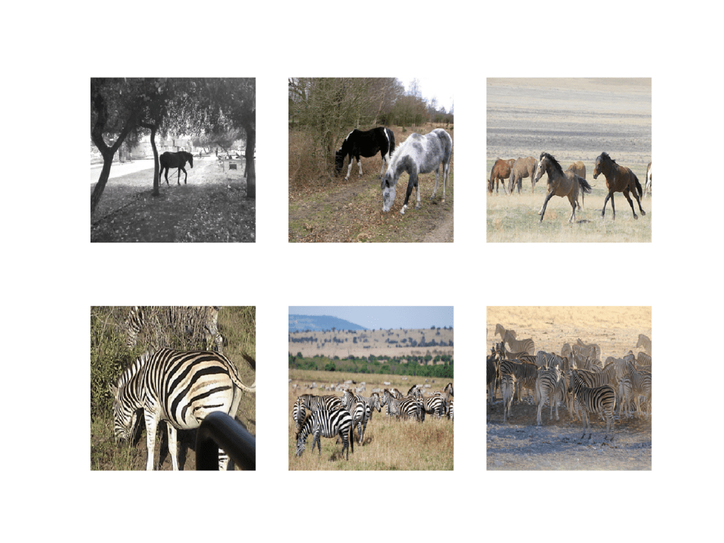
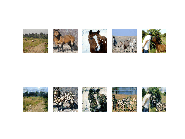
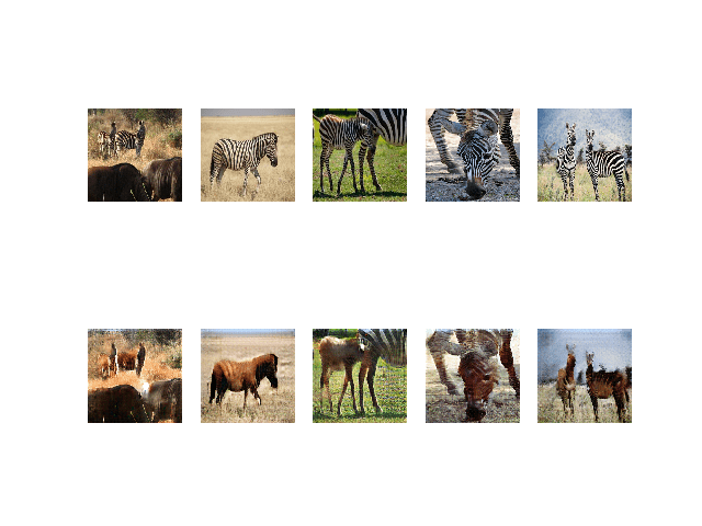
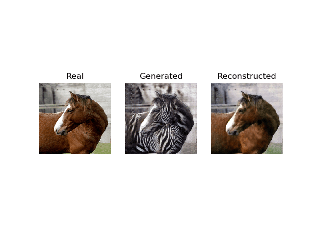
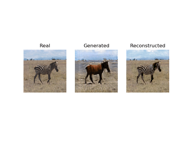
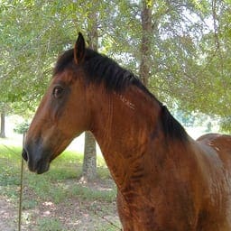
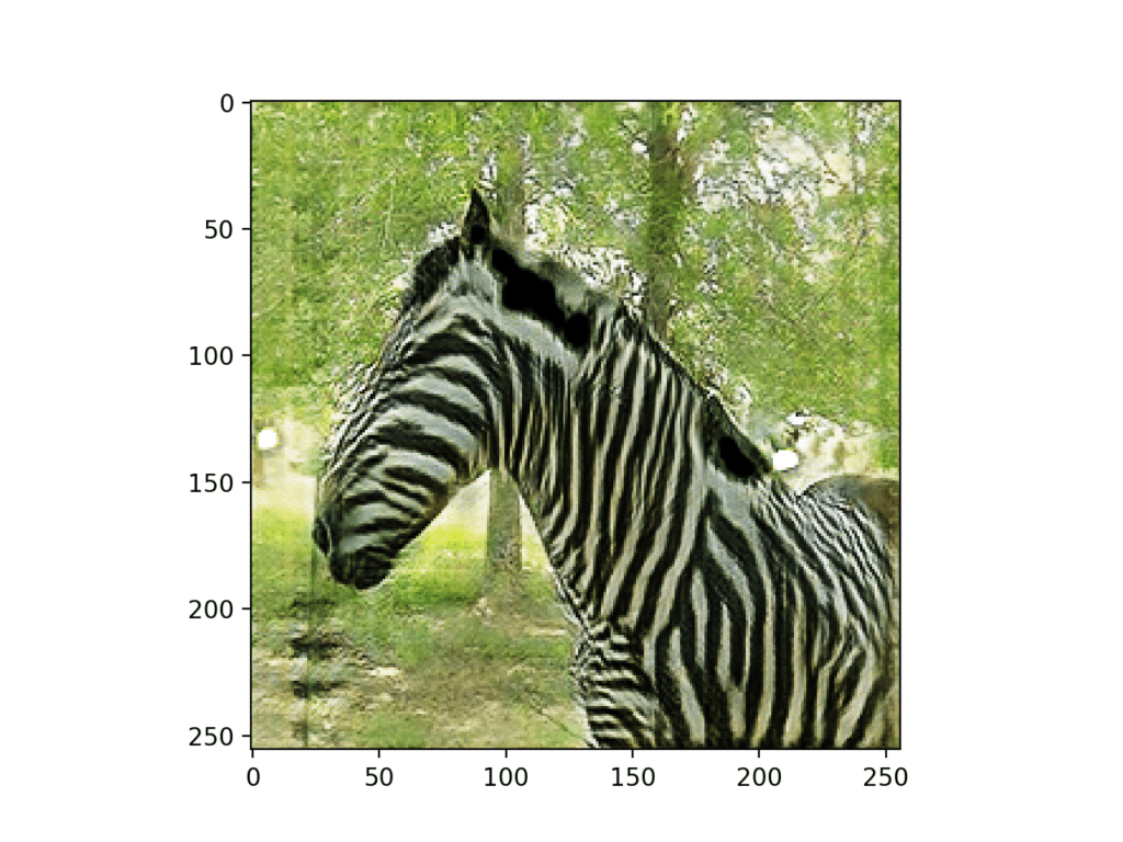


Hello! Very nice article–I have gotten it work for Google Colab.
Can you further elucidate on why we compress the image data into npz files? Why do we need 32 bit color, further increasing the size of the original data set?
Nice work!
Thanks. No need to use npz, I use that format because it is convenient and because raw pixels can take up a lot of space!
Thank you for your great tutorial.
Do you have a plan to write a starGAN tutorial with Keras like this cycleGAN tutorial?
Good question, I may cover it in the future.
Please, put starGAN tutorial with Keras on your radar. Thank you.
Thank you for the suggestion.
How to use multiple gpu’s to train the model?
Good question. I hope to cover that topic in the future.
Nice article, i am writing already asked question but if you provide multi-gpu version of CycleGAN , it will be very helpful because many models are developed on top of cycleGAN like UNIT,MUNIT,starGAN and DRIT. it will cover almost all of them. thanks
Thanks for the suggestion!
I really appreciate your nice article.
I have 2 questions.
first, in this article, the default training is 100 epochs but pytorch implementation is 200. Do I have to chenge n_epochs? or these implementation is same?(the difference is only the count, right?)
second, the original pytorch implementation seems like faster than this implementation.
this means the original implementation is optimized for training? or the difference by platform performance?
You can change the number of epochs if you want.
Yes, I expect my implementation is not as efficient as it could be.
@Ebix, can you please provide a link for the original pytorch implementation!
See the “Further Reading” of the tutorial.
Are the package versions used for the code available somewhere? I am, particularly, looking for the tensorflow version for the exact code of the tutorial.
I end up with a number of deprecation warnings, and an error while saving the model at the end, in the “model.save(filename)” lines.
Examples work with Keras 2.3 and TF2.
Thank you for the great article, everything is very clearly explained! I am working with single channel tiff images that have varying pixel values, going up to more than 300. How can I scale pixel values to the range [-1,1]? Thank you for your help!
Thanks.
This may help:
https://machinelearningmastery.com/how-to-manually-scale-image-pixel-data-for-deep-learning/
And this:
https://machinelearningmastery.com/how-to-normalize-center-and-standardize-images-with-the-imagedatagenerator-in-keras/
I tried to run the code with 1 channel tiff images, but I received an error saying “ValueError: Depth of output (64) is not a multiple of the number of groups (3) for ‘model_4/conv2d_51/convolution’ (op: ‘Conv2D’) with input shapes: [?,?,?,3], [4,4,1,64].” for the line
“c_model_AtoB = define_composite_model(g_model_AtoB, d_model_B, g_model_BtoA, image_shape”
The full error message is as follows:
/base_layer.py in __call__(self, inputs, **kwargs)
449 # Actually call the layer,
450 # collecting output(s), mask(s), and shape(s).
–> 451 output = self.call(inputs, **kwargs)
452 output_mask = self.compute_mask(inputs, previous_mask)
453
/usr/local/lib/python3.6/dist-packages/keras/engine/network.py in call(self, inputs, mask)
568 return self._output_tensor_cache[cache_key]
569 else:
–> 570 output_tensors, _, _ = self.run_internal_graph(inputs, masks)
571 return output_tensors
572
/usr/local/lib/python3.6/dist-packages/keras/engine/network.py in run_internal_graph(self, inputs, masks)
725 kwargs[‘mask’] = computed_mask
726 output_tensors = to_list(
–> 727 layer.call(computed_tensor, **kwargs))
728 output_masks = layer.compute_mask(computed_tensor,
729 computed_mask)
/usr/local/lib/python3.6/dist-packages/keras/layers/convolutional.py in call(self, inputs)
169 padding=self.padding,
170 data_format=self.data_format,
–> 171 dilation_rate=self.dilation_rate)
172 if self.rank == 3:
173 outputs = K.conv3d(
/usr/local/lib/python3.6/dist-packages/keras/backend/tensorflow_backend.py in conv2d(x, kernel, strides, padding, data_format, dilation_rate)
3938 strides=strides,
3939 padding=padding,
-> 3940 data_format=tf_data_format)
3941
3942 if data_format == ‘channels_first’ and tf_data_format == ‘NHWC’:
/usr/local/lib/python3.6/dist-packages/tensorflow_core/python/ops/nn_ops.py in convolution(input, filter, padding, strides, dilation_rate, name, data_format, filters, dilations)
896 data_format=data_format,
897 dilations=dilation_rate,
–> 898 name=name)
899
900
/usr/local/lib/python3.6/dist-packages/tensorflow_core/python/ops/nn_ops.py in convolution_internal(input, filters, strides, padding, data_format, dilations, name, call_from_convolution)
1007 data_format=data_format,
1008 dilations=dilations,
-> 1009 name=name)
1010 else:
1011 if channel_index == 1:
/usr/local/lib/python3.6/dist-packages/tensorflow_core/python/ops/gen_nn_ops.py in conv2d(input, filter, strides, padding, use_cudnn_on_gpu, explicit_paddings, data_format, dilations, name)
1069 padding=padding, use_cudnn_on_gpu=use_cudnn_on_gpu,
1070 explicit_paddings=explicit_paddings,
-> 1071 data_format=data_format, dilations=dilations, name=name)
1072 _result = _op.outputs[:]
1073 _inputs_flat = _op.inputs
/usr/local/lib/python3.6/dist-packages/tensorflow_core/python/framework/op_def_library.py in _apply_op_helper(self, op_type_name, name, **keywords)
792 op = g.create_op(op_type_name, inputs, dtypes=None, name=scope,
793 input_types=input_types, attrs=attr_protos,
–> 794 op_def=op_def)
795
796 # Conditionally invoke tfdbg v2’s op callback(s).
/usr/local/lib/python3.6/dist-packages/tensorflow_core/python/util/deprecation.py in new_func(*args, **kwargs)
505 ‘in a future version’ if date is None else (‘after %s’ % date),
506 instructions)
–> 507 return func(*args, **kwargs)
508
509 doc = _add_deprecated_arg_notice_to_docstring(
/usr/local/lib/python3.6/dist-packages/tensorflow_core/python/framework/ops.py in create_op(***failed resolving arguments***)
3355 raise TypeError(“Input #%d is not a tensor: %s” % (idx, a))
3356 return self._create_op_internal(op_type, inputs, dtypes, input_types, name,
-> 3357 attrs, op_def, compute_device)
3358
3359 def _create_op_internal(
/usr/local/lib/python3.6/dist-packages/tensorflow_core/python/framework/ops.py in _create_op_internal(self, op_type, inputs, dtypes, input_types, name, attrs, op_def, compute_device)
3424 input_types=input_types,
3425 original_op=self._default_original_op,
-> 3426 op_def=op_def)
3427 self._create_op_helper(ret, compute_device=compute_device)
3428 return ret
/usr/local/lib/python3.6/dist-packages/tensorflow_core/python/framework/ops.py in __init__(self, node_def, g, inputs, output_types, control_inputs, input_types, original_op, op_def)
1768 op_def, inputs, node_def.attr)
1769 self._c_op = _create_c_op(self._graph, node_def, grouped_inputs,
-> 1770 control_input_ops)
1771 # pylint: enable=protected-access
1772
/usr/local/lib/python3.6/dist-packages/tensorflow_core/python/framework/ops.py in _create_c_op(graph, node_def, inputs, control_inputs)
1608 except errors.InvalidArgumentError as e:
1609 # Convert to ValueError for backwards compatibility.
-> 1610 raise ValueError(str(e))
1611
1612 return c_op
ValueError: Depth of output (64) is not a multiple of the number of groups (3) for ‘model_4/conv2d_51/convolution’ (op: ‘Conv2D’) with input shapes: [?,?,?,3], [4,4,1,64].
I would really appreciate your help, thank you!
Sorry to hear that, I have some suggestions here:
https://machinelearningmastery.com/faq/single-faq/why-does-the-code-in-the-tutorial-not-work-for-me
Thank you so much Jason, Great tutorial !
I have an error like when checking target: expected model_51 to have shape (14, 12, 1) but got array with shape (14, 14, 1)
If you have an idea , i would be very happy to hear that.
You’re welcome.
Sorry to hear that, perhaps this will help:
https://machinelearningmastery.com/faq/single-faq/why-does-the-code-in-the-tutorial-not-work-for-me
Hi Jason, I’ve just finished studing the code, I’m a nubie at python, so it took me about 2 months to understand what every operation in every line means
So I finally stacked everything together for training
The training runs fine on different CPUs of my linux and Windows 10 .
But when I try to tun it on my 1060 of my Windows 10 (With all the Cudas, cuDNNs, tf 1.14 installed) I get the error
Resource exhausted: OOM when allocating tensor with shape [1,2560,64,64]
I’ve tried CUDA 9 and 10 – I get the same error
is it a normal tensor shape ?
Sorry to hear that. It might be an issue with your environment?
Perhaps try reducing the batch size?
Perhaps try running on EC2:
https://machinelearningmastery.com/develop-evaluate-large-deep-learning-models-keras-amazon-web-services/
Hi, thx for the hints and for the great tutorial!
about the batch size, you wrote there before defining train fcntion
The batch size is fixed at one image to match the description in the paper and the models are fit for 100 epochs
So the batch size is already 1 image…
My gtx 1060 has 3 gb . That’s a pitty that tensorflow can’t distribute the process with ram…
I see.
Perhaps try scaling down the images and the model in turn?
Yeah… That is one of the options…
I just came back to this page to ask you what should I change in code, when I change the resolution… Should the number of filters for example be changed, if I want to train the network on 128×128 or 512×512 res images
Or will it fully automatically adopt to new resolution?
I actually have 5 PCs with Xeon and i7 processors, so I’ve started digging https://www.tensorflow.org/tutorials/distribute/multi_worker_with_keras
Perhaps you tried converting the code for multimachine learning already? If yes,could you please make a tutor about converting the training function to run it on multiple PCs in the local Network ?
Thank you so much
I believe you will have to adapt it for different resolution images. Some experimentation may be required.
Sorry, I don’t have tutorials on distributed machine learning.
Hi Jason, thanks again
Already tested – it finally works. I had to reformat all images to 128×128, and I found
” This can easily be changed to the 6-resnet block version by setting image_shape to (128x128x3) and n_resnet function argument to 6. ”
This line where you say that we should decrease the resnet blocks number for lower res images. (from 9 for 256×256 to 6 for 128×128)
Did this coefficient of 1.5 (0.75) for resolution doubeling came to you by testing?
I guess that the higher the resolution – the stronger the filtering – is this so? If this is correct, what else should I consider changing right after resnet blocks number?
Well done.
No, the implementation is based on the paper I believe.
@Arthur, how long did it take you to do the training on your CPU?
Dear Jason,
Thanks for the nice tutorial. I implemented your code on my dataset (medical images from two different domains). I see a problem of ‘reverse effect’ i.e. the background colour of the generated image should be white instead of black (similar to source image).
Any suggestions. Thank you.
Interesting.
I have seen this sometimes too. Perhaps try re-fitting the model?
I want to ask about image dimensions.
If I use the same model with input dimensions smaller than 256*256 , would it have any impact on the quality of output?
Yes, larger images are harder to generate and may require a larger model with more training.
GPU Dedicated RAM goes full only in defining discriminator & generator. Any help how can I avoid this.
My GPU’s RAM is 6 GB
Perhaps use a smaller model?
Perhaps use smaller images?
Perhaps train on an EC2 instance?
Really cool!
On my machine it takes so long… how can I add checkpoints? So I can restart where I left
In the code i cannot see any ModelCheckpoint()
Where should I add it?
For this if:
if (i+1) % (bat_per_epo * 5) == 0:
Change to:
if True
ok got it, but how can I load the previous?
For example I generate a 200.h5 and 300.h5 file… then power off… after one day how can I resume training from 300.h5 file and keep going?
load_model(filename)
See this for more help:
https://machinelearningmastery.com/save-load-keras-deep-learning-models/
Sorry, can you resume training from 300.h5 file and keep going? can you give advice, how to do it?
Yes, load the model and train as before.
I tried to load the checkpoint as you instructed using the following:
cust = {‘InstanceNormalization’: InstanceNormalization}
g_model_AtoB = load_model(‘g_model_AtoB_005935.h5’, cust)
g_model_BtoA = load_model(‘g_model_BtoA_005935.h5’, cust)
and I run into the error
ValueError: The name “functional_3” is used 2 times in the model. All layer names should be unique.
when calling
model = Model([input_gen, input_id], [output_d, output_id, output_f, output_b])
how do I load it and continue training successfully?
I am loading this in place of the generator should I load this after the composite?
Im still looking for this answer.How can we continue the training from checkpoint or h5 model? .
I have the same issue as Mr.Jones…. Hope Mr.Brownlee can help…
You will need to write custom code, but you load the model and continue the training loop as before.
thanks for your work. if i only want to train dataset with 1 channel(256*256*1 or 512*512*1). what should i modify the code? thanks aganin
Perhaps the input to the discriminator and output of the generator.
thanks for your answer, the input is as same as the shape of training data, I modified the out put of generator(outpatch = conv2d(1,(4,4……..). However the code running failed, I wonder that it involves restnet_block adjustment.
It may. I recommend experimenting and review the output of layer summary() to see how the shapes are changing.
the generator output shape: activation_180 (Activation) (None, 256, 256, 1) 0
ResourceExhaustedError: OOM when allocating tensor of shape [512] and type float
[[node instance_normalization_336/Const (defined at /home/istbi/anaconda3/envs/tf/lib/python3.6/site-packages/keras/backend/tensorflow_backend.py:408) ]]
output shape of generator seams right, but It does not yet.
Looks like you ran out of RAM, try on an EC2 instance with more RAM?
thanks I think u are right, i run the code on jupyter notebook. I stopped the kernel. but it didn’t release the RAM. Now i seems work well . Really appreciate with your help
Well done.
I have a query.
Shall we not compile the generator model in the define_generator() function?
No need.
Is there any way of using a data generator in GANs?
The generator can be used directly, yes.
We do exactly this at the end of the tutorial.
sorry, but I have the dataset with the resolution – 128×128, it is important or not for work with your model?
Images are 256×256.
If you have images of a different size, you can resize them or change the models.
thank you so much, for your answer. it is mean, that i need only change n_resnet from 9 to 6 in –
def define_generator(image_shape, n_resnet=9)?
Sorry, in your code, we can save the model, but my GPU ONLY 6 Gb, CAN I SAVE THE WEIGHT and continue to train the model in another day?
Yes. There are exampels of saving/loading models in the above tutorial.
Dr. Jason thank you for your answer, now I can load the model, but don’t know how after that continue training, can you give me advice
I did how you recommended, and make the next script
g_model_AtoB=load_model(‘g_model_AtoB_0001300.h5′)
g_model_BtoA=load_model(g_model_BtoA_000130.h5’)
g_model_AtoB.summary()
g_model_BtoA.summary()
train(d_model_A, d_model_B, g_model_AtoB, g_model_BtoA, c_model_AtoB, c_model_BtoA, dataset)
but without any success
You can use the same training procedure as you used before.
Sorry, i have the next result after 20 epoch –
dA[0.000,0.000] dB[0.000,0.000] g[0.599,0.812]
it is mean that i need start again?
Perhaps.
sorry – we have the next losses – dA_loss1,dA_loss2, dB_loss1,dB_loss2, g_loss1,g_loss2
but where is it – Adversarial Losses ?
From the tutorial:
They are all adversarial loss values.
Hello!!! thank you, perfect article
please help me understand, can I use one model for training several objects ? for example one model for transform apple to orange and horse to zebra
Today, I have the plan to train with dataset apple and orange,
next day – zebra to horse
Probably not, this model is designed to specific transforms.
Hey, so you’re using concatenate() in the ResNet implementation here and add() in the article you linked. Can you explain what difference this usage would make?
I tried to match the paper and the pytorch implementation in this case.
thanks for your work,
sorry I have the next result –
30032, dA[0.002,0.001] dB[0.003,0.007] g[2.713,2.400] – looks good))
but in fact, the output picture looks same like and the input picture, Mr. Jason, can you recommend ьу, what I can change in the model?
horse photo input and horse photo output
Perhaps try running the example again or for longer?
Jason, thank for your quick answer.
in fact, I use the private dataset,
I try to start again already 3 times, spend much time, but result same
i sure that your code is good because in other the private datasets your model works without problem
but now, I don’t know that can do, if I continue training I will receive the next result –
>1197, dA[0.000,0.000] dB[0.000,0.000] g[0.953,0.819]
but received image is not good
i changed model.compile(loss=’mse’, optimizer=Adam(lr=0.0002, beta_1=0.5), loss_weights=[0.8]) # and loss_weights=[0.3] but result the same
in my case, it looks like discriminator works not correct, but which settings i can change?
Perhaps try making changes to the model, e.g. smaller/larger and see if it has an effect on the generated images?
Hi Mark,
Were you able to find any solution to your problem?, even I am facing the same issue with my private dataset and couldn’t find any solution to it yet. It would be really helpful if you would be able to share you findings. Thanks in advance.
I’m getting through about 750 to 800 iterations per hour, is this very slow? This is using Colab with GPU compute – I’m just wondering if this is a normal training speed, and just curious if there is a particular part of cycleGAN training (or something within Colab) which could be a bottleneck
Many thanks for the tutorials and explanations, they are very helpful!
Well done!
Perhaps explore an ec2 p3 instance?
My bad – I think the GPU switch on Colab didn’t apply at first, I restarted the Colab page and ran again and now its going at about 3100 instances per hour.
Does anyone know if this is still a slow rate for this? Curious if you happen to know the approximate speed on ec2
Thanks!
Nice work!
I am also getting around 900 instances per hour on colab and GPU runtime. Did u do anything else to speed it up?
Hey Jason,
I am using your model and running on summer2winter_Yosemite datasets.
So just wanted to know whether with the same parameters of yours can I run my model ?or for this datasets I have to use some other model or parameters. If I can use this model then what are all the parameter you suggest that I will change for getting a better result?
You may need to tune the model to the dataset.
Try adjusting the model architecture and training parameters.
My model runs in to 0 discriminator error as early as the 25th epoch – I am running with 6 resnet blocks. What could be the possible scenario?
Sounds like it might have failed. Perhaps try running again, perhaps try tuning the architecture/training configuration?
Hello Jason, I am sorry if I seem to be spamming your blogs. I have implemented a 9 resnet block cycle gan, and I am training the model on the summer 2 winter dataset. I found the discriminator loss to be heading dangerously close to 0 for a sustained period of time right from the 8th or 9th epoch and so I modified the discriminator learning rate to a really low value of .000002. Even then the discriminator loss is in the second decimal values of around 0.06-0.1 by the 5th epoch. I am not sure how to proceed. If you can guide me a bit it might be helpful. Thanks a tonne for all your resources.
Perhaps try small changes to the architecture or the learning algorithm and review the effects.
Hello Jason, thanks a tonne for your help. I figured out what the problem is and it was that in the final Cs7-1-3 layer before the tanh activation I also had the relu activation on in the generator. After this I had the tanh activation which had caused the issue.
Well done!
Hello Dr. Jason, thank you for this beautiful piece.
I am getting the folllowing error:
ResourceExhaustedError: OOM when allocating tensor with shape[1,128,128,64] and type float on /job:localhost/replica:0/task:0/device:GPU:0 by allocator GPU_0_bfc
[[{{node model_9/conv2d_101/BiasAdd-0-0-TransposeNCHWToNHWC-LayoutOptimizer}}]]
Hint: If you want to see a list of allocated tensors when OOM happens, add report_tensor_allocations_upon_oom to RunOptions for current allocation info.
[Op:__inference_keras_scratch_graph_94089]
Any advice for me? Thanks
Looks like you’re out of RAM, try an AWS EC2 with more RAM, or change the data/model to be smaller.
Many thanks for your kind response Dr. Jason. Is changing data/model similar to reducing the batch size? I will love to get some explanation on this from you!!
No.
The batch size effects the rate of learning.
Changing the model changes a lot more, e.g. how learning is performed and what is learned.
FYI,
I have Intel Dual Core 3.4GHz CPU and 3G RAM. I am using Python 2.7. I reduced the sample training size from some 1067 images to 500 images for both A and B. I run your first batch code which is downloading images and displaying without a problem. The second batch, I run all the code except the last one which is train models. The code was running for 15 minutes then gave a warning which is :
python2.7/site-packages/keras/engine/training.py:478: UserWarning: Discrepancy between trainable weights and collected trainable weights, did you set
model.trainablewithout callingmodel.compileafter ?‘Discrepancy between trainable weights and collected trainable’
Then after that, after 20 minutes the kernel died.
I believe Kernel dies due to package call for function of cpu that is not present on my cpu.
I guess my PC is not up for the task.
Nevertheless, this site is well written and pedagogical.
Regards.
You can ignore the warning.
Perhaps try python 3.
Ensure you are running from the command line directly:
https://machinelearningmastery.com/faq/single-faq/how-do-i-run-a-script-from-the-command-line
Hi Jason, thanks once again. What is the significance of running directly from the command line?
Running in an IDE/Notebook causes all kinds of issues for many readers:
https://machinelearningmastery.com/faq/single-faq/why-dont-use-or-recommend-notebooks
Running from the command line just works for everyone:
https://machinelearningmastery.com/faq/single-faq/how-do-i-run-a-script-from-the-command-line
Thanks Jason for suggestions, I did as you suggested except I was still using python 2.7.18 64bit. I run your code from command line directly. It works, except that it run very slowly. You can say now that it works on old system pc (dual core) cpu only and python 2 as well. By looking at the epoch and steps during the epoch calculation time, I calculated that it will take me about 4 months to do all 11,000 epoch. So I stopped the PC after two epochs. Python 3 is only 1.3 times faster than python 2, not enough to reduce it to one day. If possible, I will try pypy but I doubt the improvement in speed. Unless, the code has some opportunities to reduce the time needed for calculations such as reducing the batch size (steps per epoch) or epoch needed.
Try running on GPUs via EC2 to speed it up:
https://machinelearningmastery.com/develop-evaluate-large-deep-learning-models-keras-amazon-web-services/
Sorry, I used python 2.7.14 instead 2.7.18
I recommend python 3.6.
Hey Jason
Thanks for all the information on this website. It really helps. I have a query, if you may help.
I’m saving all 6 models, discriminator, generator, and composite and loading then again upon continuing training.
Is this right way, or should I just save and load generator models only?
Cause during training, the value of dA and dB falls below 0.000__.
You’re welcome.
You can save them all if you like. No need though, see the save_models() function.
Yes, save_model() only saves generator models.
So the training shall resume fine irrespective of me using model.load() for all models.
fn = “022553”
cust = {‘InstanceNormalization’: InstanceNormalization}
d_model_A = define_discriminator(image_shape)
d_model_A = load_model(“/content/drive/My Drive/cycleGan/Horses&Zebra/TrainingFiles/d_model_A_”+fn+”.h5″,cust)
d_model_B = define_discriminator(image_shape)
d_model_B = load_model(“/content/drive/My Drive/cycleGan/Horses&Zebra/TrainingFiles/d_model_B_”+fn+”.h5″,cust)
g_model_AtoB = define_generator(image_shape)
g_model_AtoB = load_model(“/content/drive/My Drive/cycleGan/Horses&Zebra/TrainingFiles/g_model_AtoB_”+fn+”.h5″,cust)
g_model_BtoA = define_generator(image_shape)
g_model_BtoA = load_model(“/content/drive/My Drive/cycleGan/Horses&Zebra/TrainingFiles/g_model_BtoA_”+fn+”.h5″,cust)
c_model_AtoB = define_composite_model(g_model_AtoB, d_model_B, g_model_BtoA, image_shape)
c_model_AtoB = load_model(“/content/drive/My Drive/cycleGan/Horses&Zebra/TrainingFiles/c_model_AtoB_”+fn+”.h5″,cust)
c_model_BtoA = define_composite_model(g_model_BtoA, d_model_A, g_model_AtoB, image_shape)
c_model_BtoA = load_model(“/content/drive/My Drive/cycleGan/Horses&Zebra/TrainingFiles/c_model_BtoA_”+fn+”.h5″,cust)
Then what else may have caused training error? I have tried restarting training many times. Anything that may help me train?
Ah I see. Yes, you will need to save all the models, then later load them all.
Sorry, you will have to prepare the function yourself, I don’t have the capacity to write it for you.
Thank you, I just wanted to confirm I’m going in the right direction regarding saving and loading model.
However, I do get a warning while loading the discriminator model, ‘No training configuration found in save file: the model was *not* compiled’.
You can safely ignore that warning.
Right! Thank you for your help.
You’re welcome.
Sir i have found difficulty in installing keras-contrib?? I create an environment in anaconda in which all libraries are installed..
But how can I install keras-contrib in that conda environment??
Step#1: I activate the environment ,and I paste a following command ,
sudo pip install git+https://www.github.com/keras-team/keras-contrib.git
it gives me error that “‘sudo’ is not recognized as an internal or external command,
operable program or batch file”.
I used another cmmand which is ,
git clone https://www.github.com/keras-team/keras-contrib.git
and again it gives me error.
‘git’ is not recognized as an internal or external command,
operable program or batch file.”
ERROR: Cannot find command ‘git’ – do you have ‘git’ installed and in your PATH?
Sir please just guide me?? I have keras version is keras-2.3.1..With tensorflow 1.14.
Perhaps you don’t support sudo on your machine, e.g. your on windows.
Try without the sudo command.
Dear Jason,
Thank you for the very useful tutorial. I was trying to add an extension for learning rate decay to the training process for another 100 epochs (total 200) and I would like to ask you some questions.
Should I only create models (discriminator and composite model) first and compile them after the learning rate conditions like the one shown below?
list_n_steps = list(range(n_steps))
for i in list_n_steps:
if list_n_steps[i] < n_steps/2:
lr = 0.0002
else:
lr = 0.0002 – 0.0002*((i – (n_steps/2)) / (n_steps/2))
Or should I include the for loop within the 'train function' before or within the loop for enumerating epochs to update/decay learning rate?
Or using tf.keras.optimizers.schedules.LearningRateSchedule function will do the job?
Thank you.
It might be easier to manually decay the learning rate as you manually step through epochs/batches.
Thank you for this informative tutorial. I have a question.
Can you please further explain the purpose of update_image_pool() here? What happens if we train the model directly using fake images and labels? How can we use this cycle gans for achieving the feature enhancement?
You’re welcome.
The update_image_pool() helps to maintain a pool of recently generated fake images. The idea is to lessen the impact of model updates on the discriminator – to slow it all down by averaging updates for images already recently seen by the model.
Try fitting the model with and without this feature and compare the results.
Dear Jason
Big fan from Japan.
After I run the code after “Tying all of this together, the complete example of training a CycleGAN model to translate photos of horses to zebras and zebras to horses is listed below.” this sentence, there is a error : module ‘tensorflow.python.framework.ops’ has no attribute ‘_TensorLike’. I tried so many ways ( like update the tensorflow) but still the error appears. can you help me with this ? thank you so much.
Are you able to confirm that you have updated your version of Keras and Tensorflow?
Thank you so much for reply
tensorflow version : 2.3
keras version : 2.3.1
Maybe try the following versions:
tensorflow: 2.3.0
keras: 2.4.3
Also, ensure you copied the code directly and are running from the command line.
More suggestions here:
https://machinelearningmastery.com/faq/single-faq/why-does-the-code-in-the-tutorial-not-work-for-me
thank you so much, after I updated to 2.4.3 it’s solved. !
I’m happy to hear that!
Hello Dr.Jason,
I was trying cyclegan for a different dataset like from sketch/edge to images. But my training stops exactly after 25 epochs not even reaching 100. But the results are not very good, looks it can be better if trained the model further.
Do you have any suggestions? What could be the reason for this? I am using google colab.
Perhaps try training for more epochs.
I was having the same problem. Reducing the image sized from 512 to 256 allowed it to run indefinitely .
Nice!
Hi Jason, may I know where is the plots of generated images stored in since im using google colab?
—-> 1 AtoB_generated_plot_000115.png
2
3 BtoA_generated_plot_000115.png
NameError: name ‘AtoB_generated_plot_000115’ is not defined
&
—-> 1 g_model_AtoB_010925.h5
2 g_model_AtoB_011500.h5
3 …
4 g_model_BtoA_010925.h5
5 g_model_BtoA_011500.h5
NameError: name ‘g_model_AtoB_010925’ is not defined
Sorry, I have never used colab and I cannot give you advice about it.
But then where can I view the generated images?
If running on a workstation or AWS EC2 instance, the images are saved in the same directory as the code file.
Thank you so much for the detailed explanation and implementation.
How to incorporate Attention Layer in the discriminators and the generators?
There may be. Sorry I don’t have an example. Perhaps experiment.
Hi Jason, thanks for the blog, I’ve learned so much about GANs this past week from reading your articles! Do you have any resources/general rules for how to modify the architecture to work on images of different resolutions?
You’re welcome!
Not really. Change the input or output shape, then adjust number of blocks to achieve the desired size.
Hi Jason, thanks for the explanation. I wanted to ask if there are any advantages to using a Resnet over a U-net architecture in the generator model?
Regards,
Joshua
Try it and see.
Thanks for these tutorials Jason, they’re so useful. I am entirely new to python and ML.
I tried running this on SageMaker, using ml.t3.xlarge.
Everything went great until it reached:
>259, dA[0.133,0.145] dB[0.171,0.158] g[6.446,6.557]
>260, dA[0.107,0.142] dB[0.223,0.144] g[9.232,8.902].
Then it just suddenly, stops. no error msg, nothing.
Am retrying on ml.c4.8xlarge. meanwhile, what do you feel could be the cause of abruptly stopping at at 260?
Perhaps there is a problem with your server?
This example, and the blog in general, are amongst the highest quality compared to what else is out there. Thanks! So I’m running this GAN example training on a Quadro P4000 with 8 Gb and it’s shaping up for possibly 30-40 hours for the 100 epochs. Does that sound about right? And that is already 4x faster than my laptop gpu. Compared to some basic Unet’s I have run at similar image matrix which have taken comparatively far less time to converge, I guess I’m surprised at the difference with this GAN network. I’m still new to this, no instinct for it yet I suppose.
Thanks!
Sounds too long. I think it took over night on a good AWS EC2 instance.
Thanks a lot for the tutorials! Very nice work!
I have a project now and I can’t choose between pix2pix GAN and cycle GAN. Could you please help me identify?
So I have a dataset, there are two kinds of data available, one is point cloud generated by the radar device (it has rich point cloud but kind of noisy, up to 64 points, with x,y and z coordinates, so up to 64*3 = 192 every frame), the other is ground truth human keypoint data generated by some depth camera (always 25 key points of human joints, for example, head, shoulder, hands, etc., with 3 axis x, y, and z coordinates. so 25*3 = 75 is the data length for each frame). My data is pair-wise, that is to say, for each frame, I have radar data and corresponding ground truth depth camera data. And my goal is to input one frame radar and get the corresponding human joints data for that frame. I design a CNN, the result is really good. I input one frame radar data (to have the same data length always, I generate some feature map), then do some convolution and fullyconnect, finally predicts that 75 coordinates of human joints. The error for each point is really low. This shows that there is a mapping between the radar point cloud coordinates and the human joint coordinates.
However, after reading pix2pix GAN and cycle GAN, I feel like my goal is more like a style transfer. Radar point cloud -> real human joint point cloud. Since my data is pair-wise, I feel like it is more related to pix2pix GAN? But cycle GAN also seems really relevant. Two bottom line: 1) Input one frame radar point cloud data, get one frame human joints prediction. 2) The prediction error should be low, at least similar to what CNN did.
Could you please give me some advice?
Perhaps this will help:
pix2pix is appropriate when you have paired training data, cyclegan is appropriate when you do not have paired training data.
What is the meaning of this line?
g_loss2, _, _, _, _ = c_model_BtoA.train_on_batch([X_realB, X_realA], [y_realA, X_realA, X_realB, X_realA])
What are the _,_,_,_ values?
It is a python idiom marks returned values from the function call that we wish to ignore.
Great tutorial Jason!
Could you help me with what changes should be made while working with grayscale images?
ValueError: Input 0 of layer conv2d_106 is incompatible with the layer: expected axis -1 of input shape to have value 1 but received input with shape (None, 256, 256, 3)
There is a value error in line 36 while using the define composite model (–>36 c_model_AtoB = define_composite_model(g_model_AtoB, d_model_B, g_model_BtoA, image_shape)
37 # composite: B -> A -> [real/fake, B])
which seems to be this line in define_composite_model —> 11 output_d = d_model(gen1_out)
I’m not sure off hand you might have to do a little trial and error.
I did change g = Conv2D(3, (7,7), padding=’same’, kernel_initializer=init)(g)
in define_generator to
# c7s1-3
g = Conv2D(1, (7,7), padding=’same’, kernel_initializer=init)(g)
which seems to resolve an error stopping the program before
Thank you for your great tutorial..
I’m following most of your tutorials because you explain everything very clearly.. thank you for that.
I’m trying to implement this horse_to_zebra translation in Pycharm using GPU. but I’m getting this error:
‘Process finished with exit code -1073740791 (0xC0000409)’
Could you please help me solve this
Sorry, I can’t help, this tutorial is for keras/tensorflow.
Hi sir,
I am doing a CycleGAN to perform image de-hazing. My dataset contains 5800 hazy and 5800 ground truth images. The images contain a mix of indoor and outdoor scenes. Do I need to change any model parameters? If yes, how do I approach this? I would be of great help to me.
I have a i5 8th gen 12 GB RAM, will it be sufficient to train the model?
Sounds like a great project!
Perhaps experiment with different size models, different learning hyperparameters, etc.
You may need to use progressive loading, depending on whether your data fits into RAM or not.
Will you make a tutorial about Contrastive Unpaired Translation (https://github.com/taesungp/contrastive-unpaired-translation, https://arxiv.org/pdf/2007.15651)?
Thanks for the suggestion.
Hi sir,
I am performing the dehazing project using this architecture. All of my images for sure are 256×256 and have 3 channels.
But, when I define the composite models I get the following warning:
WARNING:tensorflow:Model was constructed with shape (None, 256, 256, 3) for input Tensor(“input_12:0”, shape=(None, 256, 256, 3), dtype=float32), but it was called on an input with incompatible shape (None, 512, 512, 3).
The same warning appears thrice, for each composite model:
# composite: A -> B -> [real/fake, A]
c_model_AtoB = define_composite_model(g_model_AtoB, d_model_B, g_model_BtoA, image_shape)
# composite: B -> A -> [real/fake, B]
c_model_BtoA = define_composite_model(g_model_BtoA, d_model_A, g_model_AtoB, image_shape)
What should I do in this case?
Perhaps double check your loaded image size matches your expectations.
Hi, could you teach on how to generate many reconstructed images instead of translated images? Importantly to save all the reconstructed images only into files.
Thanks for the suggestion.
Hi Jaso, very nice tutorial.
I am having problems when loading a trained model for further training for instance. I use:
c_model_AtoB=keras.models.load_model((dirpath_total+’g_model_AtoB_000020’+’.h5′),custom_objects={‘InstanceNormalization’:keras_contrib.layers.InstanceNormalization},compile=True)
c_model_BtoA=keras.models.load_model((dirpath_total+’g_model_BtoA_000020’+’.h5′),custom_objects={‘InstanceNormalization’:keras_contrib.layers.InstanceNormalization},compile=True)
I am feeding these models to the train function but get the error:
RuntimeError: You must compile your model before training/testing. Use
model.compile(optimizer, loss).Any ideas how to solve this?
Thanks
Chris
Thanks.
You can ignore that warning Chris. Or perhaps compile the model before use if you like.
Hi Jason
It is actually an error, I can not ignore it. I tried compiling by doing before calling the train function:
################
#Load the pre-trained model
################
import keras_contrib
import keras
c_model_AtoB=keras.models.load_model((‘g_model_AtoB_000025’+’.h5′),custom_objects={‘InstanceNormalization’:keras_contrib.layers.InstanceNormalization})
c_model_BtoA=keras.models.load_model((‘g_model_BtoA_000025’+’.h5′),custom_objects={‘InstanceNormalization’:keras_contrib.layers.InstanceNormalization})
opt = Adam(lr=0.0002, beta_1=0.5)
c_model_AtoB.compile(loss=[‘mse’, ‘mae’, ‘mae’, ‘mae’], loss_weights=[1, 5, 10, 10], optimizer=opt)
c_model_BtoA.compile(loss=[‘mse’, ‘mae’, ‘mae’, ‘mae’], loss_weights=[1, 5, 10, 10], optimizer=opt)
################
#Train further
################
train(d_model_A, d_model_B, g_model_AtoB, g_model_BtoA, c_model_AtoB, c_model_BtoA, trainA,trainB)
I am then getting the error:
ValueError: Dimensions must be equal, but are 256 and 16 for ‘{{node mean_squared_error/SquaredDifference}} = SquaredDifference[T=DT_FLOAT](functional_39/activation_101/Tanh, IteratorGetNext:2)’ with input shapes: [1,256,256,3], [1,16,16,1].
Any suggestions?
Thanks in advance
Perhaps these tips will help:
https://machinelearningmastery.com/faq/single-faq/why-does-the-code-in-the-tutorial-not-work-for-me
Hi Jason
How can I save “dA_loss1,dA_loss2, dB_loss1,dB_loss2, g_loss1,g_loss2” output as an excel file and draw their loss into a picture?
Thanks
Chuck
This can help you save arrays to file:
https://machinelearningmastery.com/how-to-save-a-numpy-array-to-file-for-machine-learning/
Sorry, not a picture. Draw their loss into a graph.
You can save the values to file then later load the values and plot using matplotlib.
Hi Jason,
Can we use this model for single image rain removal with unpaired data?
Why you think it cannot?
Hi jason,
I got this error. Could you post the versions of the packages that you used?
————————————————————————–
ValueError Traceback (most recent call last)
/tmp/ipykernel_50911/1939433363.py in
278 c_model_BtoA = define_composite_model(g_model_BtoA, d_model_A, g_model_AtoB, image_shape)
279 # train models
–> 280 train(d_model_A, d_model_B, g_model_AtoB, g_model_BtoA, c_model_AtoB, c_model_BtoA, dataset)
/tmp/ipykernel_50911/1939433363.py in train(d_model_A, d_model_B, g_model_AtoB, g_model_BtoA, c_model_AtoB, c_model_BtoA, dataset)
233 X_realB, y_realB = generate_real_samples(trainB, n_batch, n_patch)
234 # generate a batch of fake samples
–> 235 X_fakeA, y_fakeA = generate_fake_samples(g_model_BtoA, X_realB, n_patch)
236 X_fakeB, y_fakeB = generate_fake_samples(g_model_AtoB, X_realA, n_patch)
237 # update fakes from pool
/tmp/ipykernel_50911/1939433363.py in generate_fake_samples(g_model, dataset, patch_shape)
156 def generate_fake_samples(g_model, dataset, patch_shape):
157 # generate fake instance
–> 158 X = g_model.predict(dataset)
159 # create ‘fake’ class labels (0)
160 y = zeros((len(X), patch_shape, patch_shape, 1))
~/anaconda3/lib/python3.8/site-packages/keras/engine/training.py in predict(self, x, batch_size, verbose, steps, callbacks, max_queue_size, workers, use_multiprocessing)
1718 ‘. Consider setting it to AutoShardPolicy.DATA.’)
1719
-> 1720 data_handler = data_adapter.get_data_handler(
1721 x=x,
1722 batch_size=batch_size,
~/anaconda3/lib/python3.8/site-packages/keras/engine/data_adapter.py in get_data_handler(*args, **kwargs)
1381 if getattr(kwargs[“model”], “_cluster_coordinator”, None):
1382 return _ClusterCoordinatorDataHandler(*args, **kwargs)
-> 1383 return DataHandler(*args, **kwargs)
1384
1385
~/anaconda3/lib/python3.8/site-packages/keras/engine/data_adapter.py in __init__(self, x, y, sample_weight, batch_size, steps_per_epoch, initial_epoch, epochs, shuffle, class_weight, max_queue_size, workers, use_multiprocessing, model, steps_per_execution, distribute)
1135 self._steps_per_execution_value = steps_per_execution.numpy().item()
1136
-> 1137 adapter_cls = select_data_adapter(x, y)
1138 self._adapter = adapter_cls(
1139 x,
~/anaconda3/lib/python3.8/site-packages/keras/engine/data_adapter.py in select_data_adapter(x, y)
971 def select_data_adapter(x, y):
972 “””Selects a data adapter than can handle a given x and y.”””
–> 973 adapter_cls = [cls for cls in ALL_ADAPTER_CLS if cls.can_handle(x, y)]
974 if not adapter_cls:
975 # TODO(scottzhu): This should be a less implementation-specific error.
~/anaconda3/lib/python3.8/site-packages/keras/engine/data_adapter.py in (.0)
971 def select_data_adapter(x, y):
972 “””Selects a data adapter than can handle a given x and y.”””
–> 973 adapter_cls = [cls for cls in ALL_ADAPTER_CLS if cls.can_handle(x, y)]
974 if not adapter_cls:
975 # TODO(scottzhu): This should be a less implementation-specific error.
~/anaconda3/lib/python3.8/site-packages/keras/engine/data_adapter.py in can_handle(x, y)
208 flat_inputs += tf.nest.flatten(y)
209
–> 210 tensor_types = _get_tensor_types()
211
212 def _is_tensor(v):
~/anaconda3/lib/python3.8/site-packages/keras/engine/data_adapter.py in _get_tensor_types()
1652 def _get_tensor_types():
1653 try:
-> 1654 import pandas as pd # pylint: disable=g-import-not-at-top
1655
1656 return (tf.Tensor, np.ndarray, pd.Series, pd.DataFrame)
~/anaconda3/lib/python3.8/site-packages/pandas/__init__.py in
27
28 try:
—> 29 from pandas._libs import hashtable as _hashtable, lib as _lib, tslib as _tslib
30 except ImportError as e: # pragma: no cover
31 # hack but overkill to use re
~/anaconda3/lib/python3.8/site-packages/pandas/_libs/__init__.py in
11
12
—> 13 from pandas._libs.interval import Interval
14 from pandas._libs.tslibs import (
15 NaT,
pandas/_libs/interval.pyx in init pandas._libs.interval()
ValueError: numpy.ndarray size changed, may indicate binary incompatibility. Expected 88 from C header, got 80 from PyObject
Difficult to judge but it is a numpy version mismatch issue. See the different answers here, that might help: https://stackoverflow.com/questions/66060487/valueerror-numpy-ndarray-size-changed-may-indicate-binary-incompatibility-exp
Why does your randint() function have 3 arguments? Can you explain the generate_real_samples a bit more? Thanks.
See https://numpy.org/doc/stable/reference/random/generated/numpy.random.randint.html
that is randint(high, low, size)
Generate real sample is just to take one sample from the dataset (hence it is real) and label it as “1”.
Hi, thank you for an amazing explanation of the code! I have a question about saving the image at the end when you are loading the model in. For the last part that you showed that predicted the horse to a zebra, how can I save the image that was predicted. I wanted to do it for multiple image files in a directory. I wanted to load the images from the directory and predict them, then save them. Could you help me out? Thank you!
One easy way to do is to use imwrite function from OpenCV. See this for an example: https://stackoverflow.com/questions/26681756/how-to-convert-a-python-numpy-array-to-an-rgb-image-with-opencv-2-4
My NVIDIA Graphics card has 4GB memory, and it cannot run this code. It generated an error:
”
File “C:…\AppData\Roaming\Python\Python38\site-packages\tensorflow\python\eager\execute.py”, line 59, in quick_execute
tensors = pywrap_tfe.TFE_Py_Execute(ctx._handle, device_name, op_name,
ResourceExhaustedError: OOM when allocating tensor with shape[1,2560,64,64] and type float on /job:localhost/replica:0/task:0/device:GPU:0 by allocator GPU_0_bfc
[[node model_5/model/concatenate_8/concat_1 (defined at D:/Documents/cycleGAN_TensorFlow_Learn/cyclegan_learn.py:334) ]]
Hint: If you want to see a list of allocated tensors when OOM happens, add report_tensor_allocations_upon_oom to RunOptions for current allocation info. This isn’t available when running in Eager mode.
[Op:__inference_train_function_40064]
Errors may have originated from an input operation.
Input Source operations connected to node model_5/model/concatenate_8/concat_1:
model_5/model/instance_normalization_20/add_3 (defined at D:…\Anaconda3\lib\site-packages\keras_contrib\layers\normalization\instancenormalization.py:130)
Function call stack:
train_function
”
How can the code be optimized to run with 4GB GPU memory?
The batch size is the clue for smaller memory usage, but since this example already using the batch size of 1, probably you already hit the limit.
>121, dA[0.126,0.137] dB[0.193,0.088] g[8.342,8.463]
>122, dA[0.138,0.135] dB[0.176,0.319] g[5.520,5.516]
>123, dA[0.181,0.222] dB[0.174,0.306] g[9.752,11.930]
>124, dA[0.278,0.218] dB[0.218,0.100] g[5.664,5.779]
>125, dA[0.126,0.127] dB[0.246,0.168] g[5.832,5.657]
>126, dA[0.190,0.284] dB[0.166,0.133] g[6.018,7.683]
>127, dA[0.174,0.157] dB[0.078,0.207] g[7.381,9.247]
>128, dA[0.229,0.315] dB[0.241,0.244] g[7.182,8.070]
>129, dA[0.156,0.193] dB[0.186,0.215] g[4.946,5.454]
From >13, dA[0.989,0.453] dB[2.050,0.527] g[13.013,11.449] until now it is giving around 0 values >> is it mean that there is issue ??
Notice: the rainA is masked faces and trainB is nonMasked faces
I did not find the saved model such as:
g_model_AtoB_053415.h5
g_model_AtoB_059350.h5
…
g_model_BtoA_053415.h5
g_model_BtoA_059350.h5
Where can i find it ??
Notice: the rainA is masked faces and trainB is nonMasked faces
Hello,
Thank you for the tutorial, one question to ask:
The define_composite_model function aims to instantiate a neural network whose first output is the output of the discriminative when generated images from g_model_1 are fed to it. Shouldn’t the output of the discriminative be zero, given that the images are generated/fake and not real?
You want it to be zero. That’s the goal of training the discriminative model to identify what is fake and what is not.
Yes, I understand that. But in that case, shouldn’t the output_d be zeros?
Since the generator output fake examples? I’m really not understanding this part.
Ideally, your discriminator should say zero because the images are provided by the generator. But your goal is to make your discriminator guess WRONG by improving your generator. Hence by the time you finish, you should not see the discriminator to output zero, or otherwise you didn’t train your generator enough.
Hi
I removed environment and created new one but when i tried to install this :
sudo pip install git+https://www.github.com/keras-team/keras-contrib.git
I get this error :
return _CleanResult.from_link(link1) == _CleanResult.from_link(link2)
AttributeError: type object ‘_CleanResult’ has no attribute ‘from_link’
I google it and they said :
This looks like yet another Python patch-level typing incompatibility.
Any solution please !!
I wast couple of days trying to run this code but i could not
If you can’t use that version, try to use the one from tensorflow. You do “pip install tensorflow_addons” and then use these headers:
/anaconda3/envs/tensorflow_p36/bin/python setup.py install
in my anaconda3/envs/myEnvNAme/ …. i dont have bin and python folders to install setup.py in it ..
Any advices??
You need to find the path for your python interpreter in your anaconda environment. The command line here is just an example.
Hi, could you guide me how to code on downloading all the reconstructed images directly? Secondly, how do I replace with randint to choose all the images rather than choose randomly?
# select a random sample of images from the dataset
def select_sample(dataset, n_samples):
# choose random instances
ix = randint(0, dataset.shape[0], n_samples)
# retrieve selected images
X = dataset[ix]
return X
Hi Robert…Thanks for asking.
I’m eager to help, but I just don’t have the capacity to debug code for you.
I am happy to make some suggestions:
Consider aggressively cutting the code back to the minimum required. This will help you isolate the problem and focus on it.
Consider cutting the problem back to just one or a few simple examples.
Consider finding other similar code examples that do work and slowly modify them to meet your needs. This might expose your misstep.
Consider posting your question and code to StackOverflow.
Hi, can you teach on how to avoid the repetition of selected samples?
def select_sample(dataset, n_samples):
# choose random instances
ix = randint(0, dataset.shape[0], n_samples)
# retrieve selected images
X = dataset[ix]
return X
Hi Robert,
The following may be of interest to you:
https://machinelearningmastery.com/introduction-to-random-number-generators-for-machine-learning/
Regards,
hi James,
Thank you very much for your tutorial. I learned lot. But when try to trained it takes long time. I have limited recourses. So could you please upload trained h5 files to for only run your code (zebra horse dataset.) I just studying and it will great help to me. So please..
Hi Methmal…We cannot provide h5 files. I would recommend that you investigate Google Colab with the GPU option and increased memory resources.
I am getting error in this line, ‘X1, X2 = data[‘arr_0’], data[‘arr_1′]’
KeyError: ‘arr_0 is not a file in the archive’
could you please help
Hi Ajinkya…Did you copy and paste the code? Also, you may want to try your implementation in Google Colab.
Thank you for your great tutorial.
unfortunately I got this Error:
Loaded (111, 256, 256, 3) (111, 256, 256, 3)
/usr/local/lib/python3.7/dist-packages/keras/optimizer_v2/adam.py:105: UserWarning: The
lrargument is deprecated, uselearning_rateinstead.super(Adam, self).__init__(name, **kwargs)
X_realA: (1, 256, 256, 3)
y_realA: (1, 16, 16, 1)
—————————————————————————
TypeError Traceback (most recent call last)
in ()
274 c_model_BtoA = define_composite_model(g_model_BtoA, d_model_A, g_model_AtoB, image_shape)
275 # train models
–> 276 train(d_model_A, d_model_B, g_model_AtoB, g_model_BtoA, c_model_AtoB, c_model_BtoA, dataset)
in train(d_model_A, d_model_B, g_model_AtoB, g_model_BtoA, c_model_AtoB, c_model_BtoA, dataset)
237 g_loss2, _, _, _, _ = c_model_BtoA.train_on_batch([X_realB, X_realA], [y_realA, X_realA, X_realB, X_realA])
238 # update discriminator A–>[real/fake]
–> 239 dA_loss1, _, _, _, _ = d_model_A.train_on_batch(X_realA, y=y_realA)
240 dA_loss2, _, _, _, _ = d_model_A.train_on_batch(X_fakeA, y_fakeA)
241 # update generator A–>B via adversarial and cycle loss
TypeError: cannot unpack non-iterable float object
I would appreciate it if you could help me with this Error.
Thank you in advance.
Hi Martian…Thanks for asking.
I’m eager to help, but I just don’t have the capacity to debug code for you.
I am happy to make some suggestions:
Consider aggressively cutting the code back to the minimum required. This will help you isolate the problem and focus on it.
Consider cutting the problem back to just one or a few simple examples.
Consider finding other similar code examples that do work and slowly modify them to meet your needs. This might expose your misstep.
Consider posting your question and code to StackOverflow.
Thank you for your help.
Problem Solved.
The code works fine and I got the results.
I wish you all the best.
Thank you for the very informative tutorial.
The outlook is better than a custom loop program using train_step subclassing.
As for the questions from “GAURAV SURESH SINGH” and “israr” in the past regarding the multiGPU implementation, has that been resolved already?
I couldn’t find the link, so could you please tell me.
Hi STN…You are very welcome! Please clarify the questions you are seeking answers to so that we may better assist you.
Thank you very much for your response.
I would like to update this code to work with multi-gpu.
Is there an implementation method to parallelize the loop of train_on_batch in training multiple models?
Alternatively, should I implement as custom training as described in the link below?
https://www.tensorflow.org/tutorials/distribute/multi_worker_with_ctl
Hello James,
Thank you for this tutorial! I am also trying to make it to multi-GPU. At first I thought it should be easy because of the explanation here https://www.tensorflow.org/guide/migrate/mirrored_strategy. However, I have not been successful yet.
Do you have the multi-GPU version of this tutorial? Also, because we are using 1 batch in the implementation, does it make sense to have multi-GPU version with 1 batch input data?
Great tutorial.
I would retrain the model but found a problem with load_model. Is says: “WARNING:tensorflow:No training configuration found in the save file, so the model was *not* compiled. Compile it manually.”
Do you have subbestions to fix it?
Thanks!
Great tutorial.
I would retrain the model but found a problem with load_model. Is says: “WARNING:tensorflow:No training configuration found in the save file, so the model was *not* compiled. Compile it manually.”
Do you have subbestions to fix it?
Thanks!
Great tutorial.
I would retrain the model but I found an error with load_model. It says:
“WARNING:tensorflow:No training configuration found in the save file, so the model was *not* compiled. Compile it manually”
and the train function doesn’t start.
If I run: “c_model_AtoB.compile(loss=’mse’, optimizer=Adam(learning_rate=0.0002, beta_1=0.5), loss_weights=[0.5])” (and the same for c_model_BtoA)
I still have problem with the train function.
Do you have suggestions?
Thank you very much
Hi Oliver…The following discussion may add clarity:
https://stackoverflow.com/questions/53295570/userwarning-no-training-configuration-found-in-save-file-the-model-was-not-c
Many thanks. I’ll go through it.
(sorry for my multiple comments, unfortunately i’m not able to remove them)
The following line is giving me error,
g_loss2, _, _, _, _ = c_model_BtoA.train_on_batch([X_realB, X_realA], [y_realA, X_realA, X_realB, X_realA])
The error is,
Data cardinality is ambiguous:
x sizes: 256, 256
y sizes: 1, 256, 256, 256
Make sure all arrays contain the same number of samples.
Can you tell me what i’m doing wrong?
Hi Nibin…The following resource may be of interest to you:
https://stackoverflow.com/questions/62253289/valueerror-data-cardinality-is-ambiguous
It is a good tutorial for me and I follow the pix2pix which is successfully running. However, I ran the CycleGan and get the running for overflow Error. I am the new learning of python and ML that I don’t know how to fix this bug. I check the version of my CUDA with 11.6, cudnn 8.3, python 3.9.7 and tensorflow 2.10.0. And I also run the programme in window 11. Which version would you prefer ? Should I need to reset the env to run the CycleGan programme? Because I think I can run the Pix2Pix tutorial that I can run the CycleGan same. In the process of setting up the environment I was getting very frustrated as it kept failing and I couldn’t find the problem.
OverflowError Traceback (most recent call last)
Cell In[25], line 8
6 d_model_A = define_discriminator(image_shape)
7 d_model_B = define_discriminator(image_shape)
—-> 8 c_model_AtoB = define_composite_model(g_model_AtoB, d_model_B, g_model_BtoA, image_shape)
9 c_model_BtoA = define_composite_model(g_model_BtoA, d_model_A, g_model_AtoB, image_shape)
10 train(d_model_A, d_model_B, g_model_AtoB, g_model_BtoA, c_model_AtoB, c_model_BtoA, dataset)
Cell In[17], line 10, in define_composite_model(g_model_1, d_model, g_model_2, image_shape)
8 input_id = Input(shape=image_shape)
9 output_id = g_model_1(input_id)
—> 10 output_f = g_model_2(gen1_out)
11 gen2_out = g_model_2(input_id)
12 output_b = g_model_1(gen2_out)
File ~\anaconda3\envs\tensorflow\lib\site-packages\keras\utils\traceback_utils.py:70, in filter_traceback..error_handler(*args, **kwargs)
67 filtered_tb = _process_traceback_frames(e.__traceback__)
68 # To get the full stack trace, call:
69 #
tf.debugging.disable_traceback_filtering()—> 70 raise e.with_traceback(filtered_tb) from None
71 finally:
72 del filtered_tb
File ~\anaconda3\envs\tensorflow\lib\site-packages\tensorflow\python\framework\tensor_util.py:455, in make_tensor_proto(values, dtype, shape, verify_shape, allow_broadcast)
453 else:
454 _AssertCompatible(values, dtype)
–> 455 nparray = np.array(values, dtype=np_dt)
456 # check to them.
457 # We need to pass in quantized values as tuples, so don’t apply the shape
458 if (list(nparray.shape) != _GetDenseDimensions(values) and
459 not is_quantized):
OverflowError: Exception encountered when calling layer “conv2d_transpose_62″ ” f”(type Conv2DTranspose).
Python int too large to convert to C long
Call arguments received by layer “conv2d_transpose_62″ ” f”(type Conv2DTranspose):
• inputs=tf.Tensor(shape=(None, 1073741824, 1073741824, 259), dtype=float32)
Sorry. I had search on google and stackflow but it has not more people get this bug. That why I will so confused of it
It is a good tutorial for me and I follow the pix2pix which is successfully running. However, I ran the CycleGan and get the running for overflow Error. I am the new learning of python and ML that I don’t know how to fix this bug. I check the version of my CUDA with 11.6, cudnn 8.3, python 3.9.7 and tensorflow 2.10.0. And I also run the programme in window 11. Which version would you prefer ? Should I need to reset the env to run the CycleGan programme? Because I think I can run the Pix2Pix tutorial that I can run the CycleGan same. In the process of setting up the environment I was getting very frustrated as it kept failing and I couldn’t find the problem.
OverflowError Traceback (most recent call last)
Cell In[25], line 8
6 d_model_A = define_discriminator(image_shape)
7 d_model_B = define_discriminator(image_shape)
—-> 8 c_model_AtoB = define_composite_model(g_model_AtoB, d_model_B, g_model_BtoA, image_shape)
9 c_model_BtoA = define_composite_model(g_model_BtoA, d_model_A, g_model_AtoB, image_shape)
10 train(d_model_A, d_model_B, g_model_AtoB, g_model_BtoA, c_model_AtoB, c_model_BtoA, dataset)
Cell In[17], line 10, in define_composite_model(g_model_1, d_model, g_model_2, image_shape)
8 input_id = Input(shape=image_shape)
9 output_id = g_model_1(input_id)
—> 10 output_f = g_model_2(gen1_out)
11 gen2_out = g_model_2(input_id)
12 output_b = g_model_1(gen2_out)
File ~\anaconda3\envs\tensorflow\lib\site-packages\keras\utils\traceback_utils.py:70, in filter_traceback..error_handler(*args, **kwargs)
67 filtered_tb = _process_traceback_frames(e.__traceback__)
68 # To get the full stack trace, call:
69 #
tf.debugging.disable_traceback_filtering()—> 70 raise e.with_traceback(filtered_tb) from None
71 finally:
72 del filtered_tb
File ~\anaconda3\envs\tensorflow\lib\site-packages\tensorflow\python\framework\tensor_util.py:455, in make_tensor_proto(values, dtype, shape, verify_shape, allow_broadcast)
453 else:
454 _AssertCompatible(values, dtype)
–> 455 nparray = np.array(values, dtype=np_dt)
456 # check to them.
457 # We need to pass in quantized values as tuples, so don’t apply the shape
458 if (list(nparray.shape) != _GetDenseDimensions(values) and
459 not is_quantized):
OverflowError: Exception encountered when calling layer “conv2d_transpose_62″ ” f”(type Conv2DTranspose).
Python int too large to convert to C long
Call arguments received by layer “conv2d_transpose_62″ ” f”(type Conv2DTranspose):
• inputs=tf.Tensor(shape=(None, 1073741824, 1073741824, 259), dtype=float32)
Hi Andy…Do you have a question we may help with? If so please narrow your query.
I am sorry. I wish to know your version of running this CycleGan. Basically, I use the 4070ti GPU and anaconda env to run. And what should I set the software to this CycleGan? Currently, I find the comment and you prefer keras 2.3 and tensorflow2. Can I all set the latest version to use? I am sorry to bother you because I was so troublesome yesterday.
Hi James,
what would be the best approach to use images with a higher resolution and also non-square images e.g. 1600x1200px.
Thanks!
Hi Daniel…The following resource may be of interst to you:
https://github.com/junyanz/pytorch-CycleGAN-and-pix2pix/issues/163
The access to the dataset is not working. Is there any way around to access the dataset?
Hi Munesh…Are you receiving an error message? That will allow us to better assist you.
The tutorial is great. But is there any good premade model architecture that can be used on custom data.
Hi Pallab…This is an open area of research. The following discussion may be of interest:
https://stats.stackexchange.com/questions/336722/transfer-learning-on-generative-adversarial-networks-gans
why you don’t compile generate model in the generate_model_class? while the discrimination model and combined model are compiled both.
Hi xuemin…Please clarify you question so that we may better guide you.
why there is model.compile in the end of the define_discrimination function, but no compile in the define_generator?
Can anyone tell which specific versions i shall have of keras, tensorflow???
versions i am having are:
python-3.12
tensorflow-2.17
keras-3.5
NumPy-1.26.4
Moreover if anyone came up with PyTorch implementation of the same as easy as this one is???
Thanks in Advance
Hi Rajesh…It looks like you’re using quite recent versions of Python, TensorFlow, Keras, and NumPy. However, there are some important considerations and recommendations to ensure compatibility and stability:
### 1. **Compatibility Check:**
– **Python 3.12**: This is a very recent release, and many packages may not yet be fully compatible with it. You might face issues with certain libraries that haven’t been updated to support Python 3.12.
– **TensorFlow 2.17**: This is a very recent version of TensorFlow. TensorFlow and Keras are tightly integrated, so the versions should generally be compatible if they were released around the same time.
– **Keras 3.5**: Keras 3.x versions are designed to work with TensorFlow 2.x. However, you should verify compatibility with TensorFlow 2.17, as sometimes the latest Keras might require a very specific TensorFlow version.
### 2. **Recommendations:**
– **Python**: Consider using Python 3.10 or 3.9 for better compatibility with more libraries. Python 3.12 is very new, and not all packages may have full support yet.
– **TensorFlow**: Ensure that TensorFlow 2.17 and Keras 3.5 are designed to work together. Check the TensorFlow and Keras release notes for compatibility. If you encounter issues, you might need to downgrade to TensorFlow 2.10-2.12, which are widely tested and stable versions.
– **NumPy**: NumPy 1.26.4 should generally be fine, but if you experience compatibility issues, you might consider downgrading to a version like 1.23.x, which is widely supported by many other libraries.
### 3. **PyTorch Implementation:**
– **PyTorch**: If you’re looking for an alternative to TensorFlow/Keras that’s equally easy to use, PyTorch is a great option. It’s known for being more intuitive, especially for researchers and those who want to have more control over their models.
– **Keras-like API in PyTorch**: While PyTorch itself doesn’t have a direct equivalent to Keras, the **
torch.nn** module is quite user-friendly and allows for easy model building. There are also libraries like **PyTorch Lightning** or **fastai** that offer higher-level abstractions similar to Keras, making it easier to implement models.### 4. **Possible Setup for PyTorch:**
– **Python 3.10**: If you decide to switch to a slightly older Python version for better compatibility.
– **PyTorch**: You can install PyTorch via pip with:
pip install torch torchvision torchaudio
– **PyTorch Lightning or fastai**: These can be installed with:
pip install pytorch-lightning # or fastai
Switching to a more stable Python version and verifying the compatibility of TensorFlow and Keras can save you from potential headaches. PyTorch is also an excellent alternative if you’re looking for something as user-friendly as Keras but with more flexibility.
Would you like guidance on how to migrate your existing TensorFlow/Keras code to PyTorch?
Thanks a lot Dr. James!!
Now, can you help me with
continue_trainoption please?During a office day, model gets trained for 15-20 epochs only. can you tell how can i resume the training from previously saved weights.
Hi Rajesh…You are very welcome! To resume training from previously saved weights in Keras for your CycleGAN, you can use the
continue_trainapproach by loading the saved model weights and restarting training from where it left off. Here’s how you can do it step by step:### Step 1: Save the Model Weights
Ensure that your training script saves the model weights after each epoch or at regular intervals. You can use the
model.save_weightsmethod to do this.For example, after each epoch in your training loop, save the weights:
python
# Saving model weights after each epoch
g_model.save_weights('g_model_weights_epoch_{:02d}.h5'.format(epoch))
d_model.save_weights('d_model_weights_epoch_{:02d}.h5'.format(epoch))
### Step 2: Load the Model Weights
When you want to resume training, you can load the previously saved weights before starting the new training session. This will allow the training to continue from the point where it left off.
Here’s how you can do it:
python
# Loading the saved weights
g_model.load_weights('g_model_weights_epoch_20.h5') # Change to the epoch you want to resume from
d_model.load_weights('d_model_weights_epoch_20.h5')
### Step 3: Continue Training
Once the weights are loaded, you can continue training as usual. Keras will start from the point where the model weights were saved.
### Example Code for Resuming Training
python# Assuming you have defined your generator and discriminator models (g_model, d_model)
initial_epoch = 20 # Set this to the epoch number you want to resume from
# Load the saved weights
g_model.load_weights('g_model_weights_epoch_{:02d}.h5'.format(initial_epoch))
d_model.load_weights('d_model_weights_epoch_{:02d}.h5'.format(initial_epoch))
# Continue training from where you left off
g_model.fit(
train_data,
epochs=100, # Total number of epochs you want to run
initial_epoch=initial_epoch, # Start from the previously completed epoch
callbacks=[...], # Any callbacks you are using (e.g., ModelCheckpoint)
...
)
### Tips:
– Make sure to set the
initial_epochparameter in thefitfunction to the epoch you are resuming from.– Use
ModelCheckpointto save your weights automatically at intervals during training.By using this approach, you can easily pause and resume your CycleGAN training from previously saved checkpoints without losing progress.
Thanks!! Will try, once done with data pre-processing and all. Actually I have large(~40GB) amount of the dataset.
I want to train this on
.tiffimages, where dataset contains Gray-scale and 3-channel images. Is this(different channel images) the reason due to I am facing issues while loading and creating array of the images?Error is
UnidentifiedImageError: cannot identify image fileHelp Please!!
Got it resolved!!
Actually, there were some 4-channel images which were causing the error.
I’m working with a dataset where most of the images have dimensions up to 1280×1280. I’m concerned that resizing these images to 256×256 might result in a loss of important information. To address this, I’m considering preprocessing the images to maintain their original size of 1280×1280, and potentially adding padding if necessary to keep the dimensions consistent. Is this a good approach? If not, what alternative methods should I consider?
Hi, I am training this model for huge dataset(thermal and optical images). after reaching around 20 epochs,
Epoch 20. Batch 6/12000, dA[0.002, 0.485] dB[0.005, 0.511] g[0.547, 0.701]this is the scenerio and while testing, it generates noisy images. this noisy pattern started fromaround epoch 5 and till 20, there are minor fluctuations in the noise.
meanwhile loss of dA, dB, and g dropped down from around ~3-4, ~3-4 and ~15-20 respectively in the range of epoch 5 to 20.
How to tackle this???
Hi rajdeep…The noisy image generation you’re observing during CycleGAN training, along with the significant drop in discriminator (dA, dB) and generator (g) losses, suggests that the model might be experiencing instability or overfitting. Here are some strategies to address the issue:
### 1. **Balance the Generator and Discriminator**
– The low discriminator losses (dA, dB) indicate that the discriminators are becoming too confident, which can overpower the generator and lead to noisy outputs.
– **Solution**: Try tuning the loss weights for the generator and discriminator. You can adjust the relative importance of the adversarial loss and cycle-consistency loss in the overall loss function.
python

     cycle_loss_weight = 10  # Example: increase cycle-consistency loss weight

     identity_loss_weight = 0.5  # Example: increase identity loss weight
### 2. **Introduce Noise Regularization**
– Adding noise to the input of the discriminators (dA, dB) can help prevent them from learning too quickly and overpowering the generator.
– **Solution**: Add Gaussian noise or label smoothing to the input of the discriminators to make them less confident and stabilize training.
python

     # Example of label smoothing (instead of 0 and 1, use values like 0.9 or 0.1)

     real_labels = 0.9

     fake_labels = 0.1
### 3. **Learning Rate Scheduling**
– As training progresses, a constant learning rate can lead to overfitting, which may explain the noisiness starting from epoch 5.
– **Solution**: Implement a learning rate decay or scheduler after a few epochs.
python

     # Example in Keras with Adam optimizer

     learning_rate_scheduler = tf.keras.optimizers.schedules.ExponentialDecay(

         initial_learning_rate=0.0002, decay_steps=10000, decay_rate=0.9)

     optimizer = tf.keras.optimizers.Adam(learning_rate=learning_rate_scheduler)
### 4. **Increase Model Regularization**
– Add dropout or instance normalization layers in the generator and discriminator networks to reduce overfitting and promote more stable training.
– **Solution**: Apply dropout to the generator’s layers (e.g., between 0.2 and 0.5) or use instance normalization instead of batch normalization, which is better suited for image generation tasks.
### 5. **Monitor the Cycle-Consistency Loss**
– The generator’s cycle-consistency loss may have decreased too much, leading to poorer quality reconstructions.
– **Solution**: Increase the weight of the cycle-consistency loss, as mentioned earlier, to prioritize preserving image features over fooling the discriminator.
### 6. **Data Augmentation**
– You might benefit from adding data augmentation (like flips, rotation, or slight scaling) to both thermal and optical images to prevent the model from overfitting to the training set.
– **Solution**: Use Keras’ image data generator to apply augmentation while loading batches.
### 7. **Generator Architecture Adjustments**
– If the generator is not strong enough to produce high-quality images, you can experiment with deeper architectures, such as increasing the number of residual blocks or channels in the generator.
### 8. **PatchGAN Discriminator**
– Ensure you’re using a PatchGAN discriminator, which helps reduce overfitting to local features rather than the entire image.
—
By applying these strategies, you should be able to stabilize your CycleGAN training and reduce the generation of noisy images. If the noise still persists, you may want to monitor the loss trends closely and adjust learning rates dynamically or introduce more regularization.
Let me know which approach you would like to explore first!
I am training this on .tif type of image dataset but it’s generating noisy image. do I need to change the format of the .tif images to .png??
or What else?
Hi rajdeep…No, you don’t necessarily need to convert the
.tifimages to.png, though image format can sometimes impact pre-processing steps like scaling and normalization. Instead, the noisy images could be due to other factors, such as:1. **Normalization and Pre-processing:**
– Ensure your
.tifimages are properly normalized before feeding them into the CycleGAN model. Since.tifimages often have higher bit-depth than.png, their pixel values might range differently (e.g., 0–65535 for 16-bit.tifversus 0–255 for 8-bit.png).– Use a normalization step to scale pixel values between 0 and 1 or -1 and 1, depending on your CycleGAN setup.
Example normalization:
python

   # Normalize to [-1, 1] range for RGB images

   image = (image / 32767.5) - 1  # assuming 16-bit .tif images
2. **Noisy Results Due to Training Setup:**
– **CycleGAN hyperparameters**: Adjust hyperparameters such as learning rate, loss function weights (e.g., cycle consistency loss), or use a more sophisticated optimizer like Adam with gradient clipping.
– **Training epochs**: CycleGANs typically require a high number of epochs to stabilize and avoid producing noisy images. If your model hasn’t trained long enough, try increasing the number of epochs.
– **Batch size**: If you’re using too small a batch size, it might lead to unstable training. Try increasing the batch size if possible.
3. **Dataset Quality:**
– Ensure that your
.tifimages are clean and preprocessed consistently. Sometimes.tifimages might have artifacts or noise that can cause noisy outputs.– Check if
.tifimages contain multiple channels (e.g., multispectral images) and convert them to RGB if needed.4. **CycleGAN Architecture Adjustments:**
– You can also try tweaking the generator and discriminator architectures. Adding dropout layers, batch normalization, or residual connections might help smooth out noisy results.
5. **Learning Rate Scheduling:**
– CycleGAN models can benefit from reducing the learning rate during training. Consider using a learning rate scheduler to adjust the learning rate as training progresses.
If these strategies don’t work, you can try converting
.tifimages to.pngor.jpegto see if that resolves the issue, but it’s more likely that the problem lies in the training process or pre-processing.Let me know if you’d like help implementing any of these steps!