The Cycle Generative adversarial Network, or CycleGAN for short, is a generator model for converting images from one domain to another domain.
For example, the model can be used to translate images of horses to images of zebras, or photographs of city landscapes at night to city landscapes during the day.
The benefit of the CycleGAN model is that it can be trained without paired examples. That is, it does not require examples of photographs before and after the translation in order to train the model, e.g. photos of the same city landscape during the day and at night. Instead, it is able to use a collection of photographs from each domain and extract and harness the underlying style of images in the collection in order to perform the translation.
The model is very impressive but has an architecture that appears quite complicated to implement for beginners.
In this tutorial, you will discover how to implement the CycleGAN architecture from scratch using the Keras deep learning framework.
After completing this tutorial, you will know:
How to implement the discriminator and generator models.
How to define composite models to train the generator models via adversarial and cycle loss.
How to implement the training process to update model weights each training iteration.
The model architecture is comprised of two generator models: one generator (Generator-A) for generating images for the first domain (Domain-A) and the second generator (Generator-B) for generating images for the second domain (Domain-B).
Generator-A -> Domain-A
Generator-B -> Domain-B
The generator models perform image translation, meaning that the image generation process is conditional on an input image, specifically an image from the other domain. Generator-A takes an image from Domain-B as input and Generator-B takes an image from Domain-A as input.
Domain-B -> Generator-A -> Domain-A
Domain-A -> Generator-B -> Domain-B
Each generator has a corresponding discriminator model.
The first discriminator model (Discriminator-A) takes real images from Domain-A and generated images from Generator-A and predicts whether they are real or fake. The second discriminator model (Discriminator-B) takes real images from Domain-B and generated images from Generator-B and predicts whether they are real or fake.
The discriminator and generator models are trained in an adversarial zero-sum process, like normal GAN models.
The generators learn to better fool the discriminators and the discriminators learn to better detect fake images. Together, the models find an equilibrium during the training process.
Additionally, the generator models are regularized not just to create new images in the target domain, but instead create translated versions of the input images from the source domain. This is achieved by using generated images as input to the corresponding generator model and comparing the output image to the original images.
Passing an image through both generators is called a cycle. Together, each pair of generator models are trained to better reproduce the original source image, referred to as cycle consistency.
There is one further element to the architecture referred to as the identity mapping.
This is where a generator is provided with images as input from the target domain and is expected to generate the same image without change. This addition to the architecture is optional, although it results in a better matching of the color profile of the input image.
Domain-A -> Generator-A -> Domain-A
Domain-B -> Generator-B -> Domain-B
Now that we are familiar with the model architecture, we can take a closer look at each model in turn and how they can be implemented.
The paper provides a good description of the models and training process, although the official Torch implementation was used as the definitive description for each model and training process and provides the basis for the the model implementations described below.
Want to Develop GANs from Scratch?
Take my free 7-day email crash course now (with sample code).
Click to sign-up and also get a free PDF Ebook version of the course.
How to Implement the CycleGAN Discriminator Model
The discriminator model is responsible for taking a real or generated image as input and predicting whether it is real or fake.
The discriminator model is implemented as a PatchGAN model.
For the discriminator networks we use 70 × 70 PatchGANs, which aim to classify whether 70 × 70 overlapping image patches are real or fake.
The architecture is described as discriminating an input image as real or fake by averaging the prediction for nxn squares or patches of the source image.
… we design a discriminator architecture – which we term a PatchGAN – that only penalizes structure at the scale of patches. This discriminator tries to classify if each NxN patch in an image is real or fake. We run this discriminator convolutionally across the image, averaging all responses to provide the ultimate output of D.
This can be implemented directly by using a somewhat standard deep convolutional discriminator model.
Instead of outputting a single value like a traditional discriminator model, the PatchGAN discriminator model can output a square or one-channel feature map of predictions. The 70×70 refers to the effective receptive field of the model on the input, not the actual shape of the output feature map.
The receptive field of a convolutional layer refers to the number of pixels that one output of the layer maps to in the input to the layer. The effective receptive field refers to the mapping of one pixel in the output of a deep convolutional model (multiple layers) to the input image. Here, the PatchGAN is an approach to designing a deep convolutional network based on the effective receptive field, where one output activation of the model maps to a 70×70 patch of the input image, regardless of the size of the input image.
The PatchGAN has the effect of predicting whether each 70×70 patch in the input image is real or fake. These predictions can then be averaged to give the output of the model (if needed) or compared directly to a matrix (or a vector if flattened) of expected values (e.g. 0 or 1 values).
The discriminator model described in the paper takes 256×256 color images as input and defines an explicit architecture that is used on all of the test problems. The architecture uses blocks of Conv2D-InstanceNorm-LeakyReLU layers, with 4×4 filters and a 2×2 stride.
Let Ck denote a 4×4 Convolution-InstanceNorm-LeakyReLU layer with k filters and stride 2. After the last layer, we apply a convolution to produce a 1-dimensional output. We do not use InstanceNorm for the first C64 layer. We use leaky ReLUs with a slope of 0.2.
The architecture for the discriminator is as follows:
C64-C128-C256-C512
This is referred to as a 3-layer PatchGAN in the CycleGAN and Pix2Pix nomenclature, as excluding the first hidden layer, the model has three hidden layers that could be scaled up or down to give different sized PatchGAN models.
Not listed in the paper, the model also has a final hidden layer C512 with a 1×1 stride, and an output layer C1, also with a 1×1 stride with a linear activation function. Given the model is mostly used with 256×256 sized images as input, the size of the output feature map of activations is 16×16. If 128×128 images were used as input, then the size of the output feature map of activations would be 8×8.
The model does not use batch normalization; instead, instance normalization is used.
Instance normalization was described in the 2016 paper titled “Instance Normalization: The Missing Ingredient for Fast Stylization.” It is a very simple type of normalization and involves standardizing (e.g. scaling to a standard Gaussian) the values on each feature map.
The intent is to remove image-specific contrast information from the image during image generation, resulting in better generated images.
The key idea is to replace batch normalization layers in the generator architecture with instance normalization layers, and to keep them at test time (as opposed to freeze and simplify them out as done for batch normalization). Intuitively, the normalization process allows to remove instance-specific contrast information from the content image, which simplifies generation. In practice, this results in vastly improved images.
The discriminator model is updated using a least squares loss (L2), a so-called Least-Squared Generative Adversarial Network, or LSGAN.
… we replace the negative log likelihood objective by a least-squares loss. This loss is more stable during training and generates higher quality results.
This can be implemented using “mean squared error” between the target values of class=1 for real images and class=0 for fake images.
Additionally, the paper suggests dividing the loss for the discriminator by half during training, in an effort to slow down updates to the discriminator relative to the generator.
In practice, we divide the objective by 2 while optimizing D, which slows down the rate at which D learns, relative to the rate of G.
This can be achieved by setting the “loss_weights” argument to 0.5 when compiling the model. Note that this weighting does not appear to be implemented in the official Torch implementation when updating discriminator models are defined in the fDx_basic() function.
We can tie all of this together in the example below with a define_discriminator() function that defines the PatchGAN discriminator. The model configuration matches the description in the appendix of the paper with additional details from the official Torch implementation defined in the defineD_n_layers() function.
1
2
3
4
5
6
7
8
9
10
11
12
13
14
15
16
17
18
19
20
21
22
23
24
25
26
27
28
29
30
31
32
33
34
35
36
37
38
39
40
41
42
43
44
45
46
47
48
49
50
51
52
53
54
# example of defining a 70x70 patchgan discriminator model
from keras.optimizers import Adam
from keras.initializers import RandomNormal
from keras.models import Model
from keras.models import Input
from keras.layers import Conv2D
from keras.layers import LeakyReLU
from keras.layers import Activation
from keras.layers import Concatenate
from keras.layers import BatchNormalization
from keras_contrib.layers.normalization.instancenormalization import InstanceNormalization
Note: the plot_model() function requires that both the pydot and pygraphviz libraries are installed. If this is a problem, you can comment out both the import and call to this function.
Running the example summarizes the model showing the size inputs and outputs for each layer.
A plot of the model architecture is also created to help get an idea of the inputs, outputs, and transitions of the image data through the model.
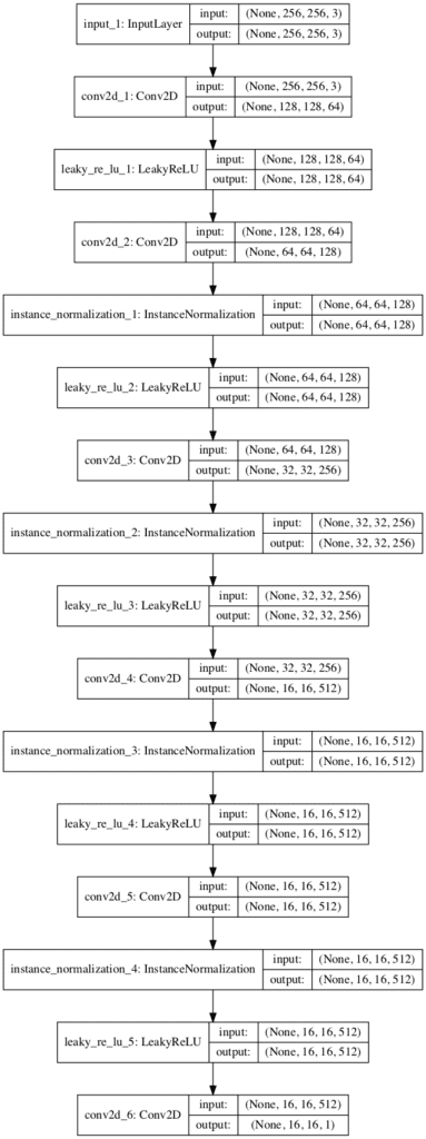
Plot of the PatchGAN Discriminator Model for the CycleGAN
How to Implement the CycleGAN Generator Model
The CycleGAN Generator model takes an image as input and generates a translated image as output.
The model uses a sequence of downsampling convolutional blocks to encode the input image, a number of residual network (ResNet) convolutional blocks to transform the image, and a number of upsampling convolutional blocks to generate the output image.
Let c7s1-k denote a 7×7 Convolution-InstanceNormReLU layer with k filters and stride 1. dk denotes a 3×3 Convolution-InstanceNorm-ReLU layer with k filters and stride 2. Reflection padding was used to reduce artifacts. Rk denotes a residual block that contains two 3 × 3 convolutional layers with the same number of filters on both layer. uk denotes a 3 × 3 fractional-strided-ConvolutionInstanceNorm-ReLU layer with k filters and stride 1/2.
First, we need a function to define the ResNet blocks. These are blocks comprised of two 3×3 CNN layers where the input to the block is concatenated to the output of the block, channel-wise.
This is implemented in the resnet_block() function that creates two Conv-InstanceNorm blocks with 3×3 filters and 1×1 stride and without a ReLU activation after the second block, matching the official Torch implementation in the build_conv_block() function. Same padding is used instead of reflection padded recommended in the paper for simplicity.
Next, we can define a function that will create the 9-resnet block version for 256×256 input images. This can easily be changed to the 6-resnet block version by setting image_shape to (128x128x3) and n_resnet function argument to 6.
Importantly, the model outputs pixel values with the shape as the input and pixel values are in the range [-1, 1], typical for GAN generator models.
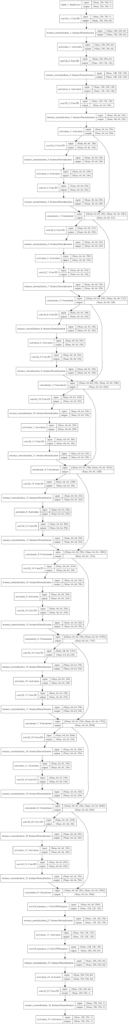
A Plot of the generator model is also created, showing the skip connections in the ResNet blocks.
Plot of the Generator Model for the CycleGAN
How to Implement Composite Models for Least Squares and Cycle Loss
The generator models are not updated directly. Instead, the generator models are updated via composite models.
An update to each generator model involves changes to the model weights based on four concerns:
Adversarial loss (L2 or mean squared error).
Identity loss (L1 or mean absolute error).
Forward cycle loss (L1 or mean absolute error).
Backward cycle loss (L1 or mean absolute error).
The adversarial loss is the standard approach for updating the generator via the discriminator, although in this case, the least squares loss function is used instead of the negative log likelihood (e.g. binary cross entropy).
First, we can use our function to define the two generators and two discriminators used in the CycleGAN.
1
2
3
4
5
6
7
8
9
10
11
...
# input shape
image_shape=(256,256,3)
# generator: A -> B
g_model_AtoB=define_generator(image_shape)
# generator: B -> A
g_model_BtoA=define_generator(image_shape)
# discriminator: A -> [real/fake]
d_model_A=define_discriminator(image_shape)
# discriminator: B -> [real/fake]
d_model_B=define_discriminator(image_shape)
A composite model is required for each generator model that is responsible for only updating the weights of that generator model, although it is required to share the weights with the related discriminator model and the other generator model.
This can be achieved by marking the weights of the other models as not trainable in the context of the composite model to ensure we are only updating the intended generator.
The first step is to define the input of the real image from the source domain, pass it through our generator model, then connect the output of the generator to the discriminator and classify it as real or fake.
1
2
3
4
5
...
# discriminator element
input_gen=Input(shape=image_shape)
gen1_out=g_model_1(input_gen)
output_d=d_model(gen1_out)
Next, we can connect the identity mapping element with a new input for the real image from the target domain, pass it through our generator model, and output the (hopefully) untranslated image directly.
1
2
3
4
...
# identity element
input_id=Input(shape=image_shape)
output_id=g_model_1(input_id)
So far, we have a composite model with two real image inputs and a discriminator classification and identity image output. Next, we need to add the forward and backward cycles.
The forward cycle can be achieved by connecting the output of our generator to the other generator, the output of which can be compared to the input to our generator and should be identical.
1
2
3
...
# forward cycle
output_f=g_model_2(gen1_out)
The backward cycle is more complex and involves the input for the real image from the target domain passing through the other generator, then passing through our generator, which should match the real image from the target domain.
1
2
3
4
...
# backward cycle
gen2_out=g_model_2(input_id)
output_b=g_model_1(gen2_out)
That’s it.
We can then define this composite model with two inputs: one real image for the source and the target domain, and four outputs, one for the discriminator, one for the generator for the identity mapping, one for the other generator for the forward cycle, and one from our generator for the backward cycle.
The adversarial loss for the discriminator output uses least squares loss which is implemented as L2 or mean squared error. The outputs from the generators are compared to images and are optimized using L1 loss implemented as mean absolute error.
The generator is updated as a weighted average of the four loss values. The adversarial loss is weighted normally, whereas the forward and backward cycle loss is weighted using a parameter called lambda and is set to 10, e.g. 10 times more important than adversarial loss. The identity loss is also weighted as a fraction of the lambda parameter and is set to 0.5 * 10 or 5 in the official Torch implementation.
1
2
3
...
# compile model with weighting of least squares loss and L1 loss
This function can then be called to prepare a composite model for training both the g_model_AtoB generator model and the g_model_BtoA model; for example:
Summarizing and plotting the composite model is a bit of a mess as it does not help to see the inputs and outputs of the model clearly.
We can summarize the inputs and outputs for each of the composite models below. Recall that we are sharing or reusing the same set of weights if a given model is used more than once in the composite model.
Generator-A Composite Model
Only Generator-A weights are trainable and weights for other models and not trainable.
Now, we can define the steps of a single training iteration. We will model the order of updates based on the implementation in the official Torch implementation in the OptimizeParameters() function (Note: the official code uses a more confusing inverted naming convention).
Update Generator-B (A->B)
Update Discriminator-B
Update Generator-A (B->A)
Update Discriminator-A
First, we must select a batch of real images by calling generate_real_samples() for both Domain-A and Domain-B.
Typically, the batch size (n_batch) is set to 1. In this case, we will assume 256×256 input images, which means the n_patch for the PatchGAN discriminator will be 16.
The paper describes using a pool of previously generated images from which examples are randomly selected and used to update the discriminator model, where the pool size was set to 50 images.
… [we] update the discriminators using a history of generated images rather than the ones produced by the latest generators. We keep an image buffer that stores the 50 previously created images.
This can be implemented using a list for each domain and a using a function to populate the pool, then randomly replace elements from the pool once it is at capacity.
The update_image_pool() function below implements this based on the official Torch implementation in image_pool.lua.
1
2
3
4
5
6
7
8
9
10
11
12
13
14
15
16
17
# update image pool for fake images
def update_image_pool(pool,images,max_size=50):
selected=list()
forimage inimages:
iflen(pool)<max_size:
# stock the pool
pool.append(image)
selected.append(image)
elif random()<0.5:
# use image, but don't add it to the pool
selected.append(image)
else:
# replace an existing image and use replaced image
ix=randint(0,len(pool))
selected.append(pool[ix])
pool[ix]=image
returnasarray(selected)
We can then update our image pool with generated fake images, the results of which can be used to train the discriminator models.
1
2
3
4
...
# update fakes from pool
X_fakeA=update_image_pool(poolA,X_fakeA)
X_fakeB=update_image_pool(poolB,X_fakeB)
Next, we can update Generator-A.
The train_on_batch() function will return a value for each of the four loss functions, one for each output, as well as the weighted sum (first value) used to update the model weights which we are interested in.
1
2
3
...
# update generator B->A via adversarial and cycle loss
Tying this all together, we can define a function named train() that takes an instance of each of the defined models and a loaded dataset (list of two NumPy arrays, one for each domain) and trains the model.
A batch size of 1 is used as is described in the paper and the models are fit for 100 training epochs.
As an improvement, it may be desirable to combine the update to each discriminator model into a single operation as is performed in the fDx_basic() function of the official implementation.
Additionally, the paper describes updating the models for another 100 epochs (200 in total), where the learning rate is decayed to 0.0. This too can be added as a minor extension to the training process.
Further Reading
This section provides more resources on the topic if you are looking to go deeper.
Hi Jason, thanks for this great tutorial about CycleGAN. I have a physics-based regression problem (~8 input features and 1 response variable) with only 35 data points from the real world lab test results. We have a 1D simulation tool with which we can generate any number of low fidelity artificial data points.
Unfortunately, the low fidelity artificial synthesised data points are not having the same distribution as the real world lab test results and there are differences due to domain shift between real world lab test and simulated data.
Can you please give some tips on applying CycleGAN for a numeric dataset (regression problem) to make the low fidelity (synthesised data) to appear more like the real world lab test data but still being physically consistent?
Hi Jason,
In my case, the 35 lab test points can be said to represent data from Domain A and the 1000s (or seemingly infinite) of points from the 1D Physics Simulator can be said to be from Domain B. I believe the scenario is similar to the case of CycleGANs generating Van Gogh style dog paintings ( https://dmitryulyanov.github.io/feed-forward-neural-doodle/ ) by combining seemingly large number of Dog photos (which are theoretically unlimited) with Van Gogh paintings which are limited in number, so I think CycleGANs are a good choice for my problem. I do have a few simple questions though:
For my scenario synthesizing numeric data is the update_image_pool function needed to keep track of fake samples created by the generator?
Do I have to employ Instance normalization or batch normalization in the architecture of the generator and discriminator?
Since I am only synthesizing numeric data, I am planning to use a simple architecture for the generator and discriminator as below, is this appropriate?
`
def define_discriminator(n_inputs=nr_features):
model = Sequential()
model.add(Dense(n_inputs, activation=’relu’, kernel_initializer=’he_uniform’, input_dim=n_inputs))
model.add(Dense(32,activation=’relu’))
model.add(Dense(1, activation=’sigmoid’))
model.compile(loss=’binary_crossentropy’, optimizer=’adam’, metrics=[‘accuracy’])
return model
def define_generator(nr_features):
model = Sequential()
model.add(Dense(nr_features, activation=’LeakyReLU’,input_shape=(nr_features,)))
model.add(Dense(32, activation=’LeakyReLU’))
model.add(Dense(1, activation=’linear’))
model.compile(loss=’mse’, optimizer=Adam(lr=0.0002, beta_1=0.5), loss_weights=[0.5])
return model
Thanks for the nice post. Just one question regarding update_image_pool function, wouldn’t be a possible issue to reach an index out of range of pool?
++ max_size is set to 50 (if len(pool) < max_size) , hence pool index are from 0 to 49.
++ ix = randint(0, len(pool)), will return an integer between 0 to 50
So there may be a possibility to access pool[50] which is out of range?
First of all, I want o thank you. I really appreciate your post, it really helped me understand the whole “CycleGan” thing, you really did a great thing explaining everything.
Secondly, I want to ask you something. Your training loop is quite different from the other implementations that I have seen(PyTorch official, Keras). Mainly, I reffer to the way you are updating the models G1, D1, G2, D2 instead of G1,G2, D1, D2. Is there any specific reason you have decided to do it this way, or it was just modified for simplicity?
Hey Jason! Thanks for the wonderful and in-depth explanation of this complex topic.
I feel a little stupid asking this but can you please tell me how we are passing the images to the code? We are supposed to feed them as lists but are those lists supposed to be made of 3-dim image data?
Thank you.
I was trying to save and load the model using Keras’ save & load_model but on loading it fails to recognize the InstanceNormalization layer. Can you suggest a workaround?
Also, any way to visualize the training images after some iterations?
Hello and thanks for the very nice tutorials! Could you please make a tutorial on how to implement a recycleGAN model for video retargeting in keras? Thanks
Due to a bug not allowing me to correctly import tensorflow addons (undefined symbol error)
which I hope to figure out at some stage, I cannot use the Instance normalization layer.
Can I just replace this with BatchNormalization (with axis -1 same as here) or do I have to do anything special in addition?
I have some questions about Res-Net architecture in the Generator model. Seems like in your res netblock, are you downsampling and upsampling every time? In the first res block, you feed in 256 x64x64 to the block and concatenate it. The result is 512x64x64. Then you feed that into the rest netblock. It becomes 256x64x64 then for concatenation it becomes 768x54x64. Usually, I thought res-net block would do elt-wise adding not concatenation.
Thanks alot for the very helpful tutorial. This helped me alot in understanding how to perform sequential training of different parts of a single model in Keras.
I have a few questions, and these might be a little stupid given the lack of my expertise in Keras:
1) If you set the discriminator as trainable=FALSE when you create the composite model, don’t you need to set it back to trainable=TRUE before running the train_on_batch of discriminator.
2) Can you expand a little bit more on how the weights are updated for layers shared between multiple models i.e the layers of the generator model which are also part of composite model. Are the layers in Keras global entities and hence can be updated as part of different models, or are the layers specific to each model?
3) When compiling the composite model, there are 4 different loss functions, i.e mae , mse.. . I wanted to ask how the order of these 4 loss functions was decided?
I am trying to use the above tutorial to write another architecture of my own which requires sequential training of various parts of the model and hence my questions.
No, the trainability only affects the scope of the model – to each call to compile(). It is trainable standalone, not trainable as part of the discriminator.
Hi,
Thank you for your in-depth explanations of the model!
I’m trying to a use the related Pix2pix model with Tensorflow and I have a question about your usage of Instance Normalization.
Tensorflow Pix2Pix tutorial uses Batch Normalization on every down(or up)sampling steps instead of Instance Normalization.
From what I understood, Instance Normalization is better than Batch Normalization for image generation, so should I use Instance Normalization in my model?
I mean, is there a reason to not use Instance Normalization over Batch Normalization (I’ll be always using a batch size of 1, if that matters)?
I think it’s what I’m going to do, it’s just that it will take quite some time to train so I’m trying to get things right before training. I’ll compare with some simpler datasets first then.
Thank you again for all the articles you made on this subject!
0%| | 0/533 [00:00<?, ?it/s]C:\Users\acer\Anaconda3\lib\site-packages\keras\engine\training.py:297: UserWarning: Discrepancy between trainable weights and collected trainable weights, did you set model.trainable without calling model.compile after ?
'Discrepancy between trainable weights and collected trainable'
C:\Users\acer\Anaconda3\lib\site-packages\keras\engine\training.py:297: UserWarning: Discrepancy between trainable weights and collected trainable weights, did you set model.trainable without calling model.compile after ?
'Discrepancy between trainable weights and collected trainable'
C:\Users\acer\Anaconda3\lib\site-packages\keras\engine\training.py:297: UserWarning: Discrepancy between trainable weights and collected trainable weights, did you set model.trainable without calling model.compile after ?
'Discrepancy between trainable weights and collected trainable'
C:\Users\acer\Anaconda3\lib\site-packages\keras\engine\training.py:297: UserWarning: Discrepancy between trainable weights and collected trainable weights, did you set model.trainable without calling model.compile after ?
'Discrepancy between trainable weights and collected trainable'
While training the model I got this warning. Do I need to take care of this or is it fine?
In the above tutorial, you have used a batch size of 1 but I am using 2, so do I need to change anything else also in the model architecture to make it give good results or changing batch_size won,t affect the results?
Actually I changed some parts of code and batch size to 4 and also the size of the image to 128. The model is getting trained and has reached the 20th epoch. I just wanted to know if the model will give good results with my batch size also?
I also did one more change to the code. Instead of loading the whole data at once I have created a custom data generator to give 4 images at a time and not using the whole memory to store the whole dataset.
So does these two changes will give me good results or not?
I am very glad and benefited by this post of yours on CycleGAN implementation. You have very lucidly explained this quite complex topic and I very much appreciate it.
I have a small doubt. In the Resnet Block creation function, while you are doing the concatenation of Input layer and g, you have written:
g = Concatenate()[g, input_layer]
Shouldn’t the argument list be [input_layer, g]? Because otherwise the input layer will come after g in the merged layer. But, it should come before g according to the architecture in the paper, isn’t it? Can u kindly clear my doubt?
many thanks for this great tutorial, it really helps to understand the basic idea behind a CycleGAN. I have one question regarding the outputs of the CycleGAN:
When I apply your implementation on the apples2oranges dataset from the official paper and inspect the outputs of the predict() method, the output quality never changes. It starts with a noisy image where the original input image used for prediction can still slightly be seen. However, even after 200 epochs, it appears the same. Despite that, the loss values decrease early but start to stagnate after 30-50 epochs.
thank you so much for the article!
the g_loss1,g_loss2 are huge (around 3000) and it doesnt converge, did you ran into this situation? i havent change the code, just fixed some import issues (random etc.)
If the generator losses are very high, you should check the color values of the images. If they’re in the range of [0..255], the losses are typically very large, whereas for normalized color values to [-1..1] or [0..1] (depending on your activation function) already reduces the loss values for the generator.
Another issue that I encountered when working with composite models was that I accidentally trained the wrong model, i.e. I used the wrong model for generating fake images.
My question might be trivial: I am training the above model (a version inspired by yours but my own code) in Google Colab. Since there are 1200 or so images in the train A folder and if I were to use 100 epochs of training, I will have to run 120000 steps of training. Now even with GPU I most likely will need at least 24 hours of model training for this model. But with the 12 hour GPU limit on Colab this seems to be impossible. So I am thinking of using model checkpoints and also note down the step at which training stopped. Would it be right if I load the model weights at the saved point and start the remaining training from the step at which it stopped?
Hi Jason, great article! Thanks for sharing it online. One doubt, why is the training pattern trains generators first and not the discriminators first, like the simple GAN models.
Hi Jason, I have read many of your articles but can you please include your own results from running this code so people can see what the end result is like and able to assess if this one is worth reading at all?
Hi,
Thank you for your informative article.
I am running it on my 3D data and the problem is the discriminator accuracy after number of steps reaches 100% which I guess is bad. Is this something common? Do you know what can be done in this case?
Except in the case of having unpaired images, what are the benefits of using CycleGAN in comparison to plain GAN? If we have paired images, is it better to use GAN?
I am asking this question because when CycleGAN used in translation tasks, it often leads to results
which lack sharpness and fine-detailed structures.
There is a MAJOR mistake in the construction of the ResNet. ResNet does not concatenate the input and the output, it adds them together. Concatenation leads to feature maps that are thousands of channels deep which slows down learning significantly. To change this all you have to do is replace concatenate with add. It is also missing a Relu at the end (the input to the next res block needs to be activated). This change makes the network have about 1/3 the number of parameters which is extremely significant.
I would definitely take another look to make sure. The paper only says it uses residual blocks. All the implementations on github that I can find for cycleGan use addition like in the ResNet paper.
It’s confusing because the torch implementation uses “concatTable” to do the skip connection while the pytorch implementation uses a straightforward + operator. Other keras implementations I’ve seen use an Add layer. Im not familiar with torch and lua, but maybe concatTable is a misleading name? Anyways, thanks for looking into it and providing a great tutorial.
Hello, I am just a noob in Artificial Intelligence.
The only few AI things that I’ve done have been done with Tensor dataset and have trained pretty quickly. WHereas, when Ive run this code, which works with Numpy Arrays, it runs very slowly. Is this an inherent problem of using NumPy arrays or may I be doing something wrong? In case it is a problem of using NumPy arrays, is there any way to change this code so that it uses tensors?
Thanks for this tutorial, it was very helpful. However, I am currently facing the common problem with GANs (mode collapse) where the discriminator loss falls to zero very quickly and the generator keeps producing the same images for different inputs. Could you please suggest any solution to address this issue?
I had question: why do we used resnet block in the generator model. In the pix2pix’s generator model, we didnt had a resnet block, then why you added it over here, if they both do the same thing (by both i mean cycle gan’s generator and pix2pix’s generator). Then why did we added a resnet block over here.
This might be a dumb question, but what do you mean when you say load a dataset as a list of two numpy arrays? I’m not really experienced and I don’t have much experience with keras.
I am getting an error while evaluating. I have a reference to “How to Develop a GAN for Generating MNIST Handwritten Digits”. I have attempted to implement the “summarize_performance” function in the “How to Implement CycleGAN Models From Scratch With Keras” But I ended with an error.
Hi Jason, thank you so much for this article.
In the “generate_real_samples” function, you choose the images randomly. I wonder why don’t we iterate the whole dataset for each epoch instead? Which one is better?
Hey, thanks so much for this article. Would you know why, the generator models output the same image provided to them as input (output them in a different quality but its the same image). I’m trying to make it work on a custom dataset.
One graphics card has 4GB GPU memory, but it cannot run this code showing OOM.
– How to adjust this code to run with the GPU?
On another computer with 6GB GPU Memory, it runs.
On both computer it shows (although runs):
”
WARNING:tensorflow:5 out of the last 7 calls to <function Model.make_predict_function..predict_function at 0x000001C0BA937310> triggered tf.function retracing. Tracing is expensive and the excessive number of tracings could be due to (1) creating @tf.function repeatedly in a loop, (2) passing tensors with different shapes, (3) passing Python objects instead of tensors. For (1), please define your @tf.function outside of the loop. For (2), @tf.function has experimental_relax_shapes=True option that relaxes argument shapes that can avoid unnecessary retracing. For (3), please refer to https://www.tensorflow.org/guide/function#controlling_retracing and https://www.tensorflow.org/api_docs/python/tf/function for more details.
WARNING:tensorflow:6 out of the last 8 calls to <function Model.make_predict_function..predict_function at 0x000001C0B22F85E0> triggered tf.function retracing. Tracing is expensive and the excessive number of tracings could be due to (1) creating @tf.function repeatedly in a loop, (2) passing tensors with different shapes, (3) passing Python objects instead of tensors. For (1), please define your @tf.function outside of the loop. For (2), @tf.function has experimental_relax_shapes=True option that relaxes argument shapes that can avoid unnecessary retracing. For (3), please refer to https://www.tensorflow.org/guide/function#controlling_retracing and https://www.tensorflow.org/api_docs/python/tf/function for more details.
”
These are warning only. So you can ignore it. But that means your code has something not native to Tensorflow so it cannot run fast. The message says it all: “could be due to (1) creating @tf.function repeatedly in a loop, (2) passing tensors with different shapes, (3) passing Python objects instead of tensors”
My version is:
CUDA = 10.2
Python = 3.7
TF-gpu = 2.3.0
Keras = 2.4.3
I fixed the conflict between the version of TF and Keras
My computer
Processor: Core i9
RAM: 64GB
GPU:2080Ti
However, I just loaded 1000 images for each domain, like (1000,400,400,3), (1000,400,400,3)
I got errors like ‘ResourceExhaustedError’
‘ResourceExhaustedError: OOM when allocating tensor with shape[16,1792,100,100] and type float on /job:localhost/replica:0/task:0/device:GPU:0 by allocator GPU_0_bfc
[[node functional_11/functional_1/concatenate_5/concat (defined at :27) ]]
Hint: If you want to see a list of allocated tensors when OOM happens, add report_tensor_allocations_upon_oom to RunOptions for current allocation info.
[Op:__inference_train_function_39883]
Errors may have originated from an input operation.
Input Source operations connected to node functional_11/functional_1/concatenate_5/concat:
functional_11/functional_1/instance_normalization_14/add_1 (defined at E:\Anaconda3\envs\YOLO-gpu\lib\site-packages\keras_contrib\layers\normalization\instancenormalization.py:130)


 From Scratch in Keras")


Hi Jason, thanks for this great tutorial about CycleGAN. I have a physics-based regression problem (~8 input features and 1 response variable) with only 35 data points from the real world lab test results. We have a 1D simulation tool with which we can generate any number of low fidelity artificial data points.
Unfortunately, the low fidelity artificial synthesised data points are not having the same distribution as the real world lab test results and there are differences due to domain shift between real world lab test and simulated data.
Can you please give some tips on applying CycleGAN for a numeric dataset (regression problem) to make the low fidelity (synthesised data) to appear more like the real world lab test data but still being physically consistent?
Good question.
Perhaps you can try adapting the above example for your data?
Perhaps try a gaussian process or kde approach to modeling the distribution of points and sample it randomly?
Hi Jason,
In my case, the 35 lab test points can be said to represent data from Domain A and the 1000s (or seemingly infinite) of points from the 1D Physics Simulator can be said to be from Domain B. I believe the scenario is similar to the case of CycleGANs generating Van Gogh style dog paintings ( https://dmitryulyanov.github.io/feed-forward-neural-doodle/ ) by combining seemingly large number of Dog photos (which are theoretically unlimited) with Van Gogh paintings which are limited in number, so I think CycleGANs are a good choice for my problem. I do have a few simple questions though:
For my scenario synthesizing numeric data is the
update_image_poolfunction needed to keep track of fake samples created by the generator?Do I have to employ
Instance normalizationorbatch normalizationin the architecture of the generator and discriminator?Since I am only synthesizing numeric data, I am planning to use a simple architecture for the generator and discriminator as below, is this appropriate?
`def define_discriminator(n_inputs=nr_features):
model = Sequential()
model.add(Dense(n_inputs, activation=’relu’, kernel_initializer=’he_uniform’, input_dim=n_inputs))
model.add(Dense(32,activation=’relu’))
model.add(Dense(1, activation=’sigmoid’))
model.compile(loss=’binary_crossentropy’, optimizer=’adam’, metrics=[‘accuracy’])
return model
def define_generator(nr_features):
model = Sequential()
model.add(Dense(nr_features, activation=’LeakyReLU’,input_shape=(nr_features,)))
model.add(Dense(32, activation=’LeakyReLU’))
model.add(Dense(1, activation=’linear’))
model.compile(loss=’mse’, optimizer=Adam(lr=0.0002, beta_1=0.5), loss_weights=[0.5])
return model
If it is just numerical data, perhaps use a gaussian process or other much simpler generative model?
Hi Jason,
Can you elaborate about batch normalization and instance normalization? Why in instance normalization, axis is set to -1.
Thanks,
Prisilla
Excellent question.
Basically, batch norm normalizes (standardizes) across the batch, instance norm normalizes (standardizes) across the instance only.
This paper explains it:
https://arxiv.org/abs/1607.08022
The axis of -1 indicates we are normalizing over channels for one image, assuming a channels-last image format. You can see this from the API documentation here:
https://github.com/keras-team/keras-contrib/blob/master/keras_contrib/layers/normalization/instancenormalization.py
I hope that helps.
Hi Jason,
Thanks for the nice post. Just one question regarding update_image_pool function, wouldn’t be a possible issue to reach an index out of range of pool?
++ max_size is set to 50 (if len(pool) < max_size) , hence pool index are from 0 to 49.
++ ix = randint(0, len(pool)), will return an integer between 0 to 50
So there may be a possibility to access pool[50] which is out of range?
Nice catch!
I should do len(pool)-1.
Nevertheless, python does not do out of bounds, an index of 50 will become an index of 0.
Hi Jason,
First of all, I want o thank you. I really appreciate your post, it really helped me understand the whole “CycleGan” thing, you really did a great thing explaining everything.
Secondly, I want to ask you something. Your training loop is quite different from the other implementations that I have seen(PyTorch official, Keras). Mainly, I reffer to the way you are updating the models G1, D1, G2, D2 instead of G1,G2, D1, D2. Is there any specific reason you have decided to do it this way, or it was just modified for simplicity?
Thank you,
Radu
Thanks Radu.
Yes, the update order of the models is based on the official implementation provided with the paper.
Hey Jason! Thanks for the wonderful and in-depth explanation of this complex topic.
I feel a little stupid asking this but can you please tell me how we are passing the images to the code? We are supposed to feed them as lists but are those lists supposed to be made of 3-dim image data?
Thank you.
No stupid questions here!
Images are loaded as numpy arrays, to learn more about this see this tutorial:
https://machinelearningmastery.com/how-to-load-and-manipulate-images-for-deep-learning-in-python-with-pil-pillow/
And here:
https://machinelearningmastery.com/how-to-load-convert-and-save-images-with-the-keras-api/
Thanks for the well explained article.
I was trying to save and load the model using Keras’ save & load_model but on loading it fails to recognize the InstanceNormalization layer. Can you suggest a workaround?
Also, any way to visualize the training images after some iterations?
Good question, use:
Hello and thanks for the very nice tutorials! Could you please make a tutorial on how to implement a recycleGAN model for video retargeting in keras? Thanks
Thanks for the suggestion!
Hi Jason, thanks for the excellent walkthrough.
Due to a bug not allowing me to correctly import tensorflow addons (undefined symbol error)
which I hope to figure out at some stage, I cannot use the Instance normalization layer.
Can I just replace this with BatchNormalization (with axis -1 same as here) or do I have to do anything special in addition?
Thanks
Not really.
You can install InstanceNormalziation as a Keras extension, not a tensorflow extension.
Or perhaps try just skipping the layer?
Hi,
I have some questions about Res-Net architecture in the Generator model. Seems like in your res netblock, are you downsampling and upsampling every time? In the first res block, you feed in 256 x64x64 to the block and concatenate it. The result is 512x64x64. Then you feed that into the rest netblock. It becomes 256x64x64 then for concatenation it becomes 768x54x64. Usually, I thought res-net block would do elt-wise adding not concatenation.
Yes, it is modified to match what was implemented in the cyclegan paper.
Hi,
Thanks alot for the very helpful tutorial. This helped me alot in understanding how to perform sequential training of different parts of a single model in Keras.
I have a few questions, and these might be a little stupid given the lack of my expertise in Keras:
1) If you set the discriminator as trainable=FALSE when you create the composite model, don’t you need to set it back to trainable=TRUE before running the train_on_batch of discriminator.
2) Can you expand a little bit more on how the weights are updated for layers shared between multiple models i.e the layers of the generator model which are also part of composite model. Are the layers in Keras global entities and hence can be updated as part of different models, or are the layers specific to each model?
3) When compiling the composite model, there are 4 different loss functions, i.e mae , mse.. . I wanted to ask how the order of these 4 loss functions was decided?
I am trying to use the above tutorial to write another architecture of my own which requires sequential training of various parts of the model and hence my questions.
You’re welcome.
No, the trainability only affects the scope of the model – to each call to compile(). It is trainable standalone, not trainable as part of the discriminator.
Yes, I cover this in another post, this one I think:
https://machinelearningmastery.com/how-to-develop-a-generative-adversarial-network-for-a-1-dimensional-function-from-scratch-in-keras/
The order matters, but is the linear order we specified.
It’s a fun model this one! Hang in there!
Hi,
Thank you for your in-depth explanations of the model!
I’m trying to a use the related Pix2pix model with Tensorflow and I have a question about your usage of Instance Normalization.
Tensorflow Pix2Pix tutorial uses Batch Normalization on every down(or up)sampling steps instead of Instance Normalization.
On the other hand, their tutorial code on github (https://github.com/tensorflow/examples/blob/master/tensorflow_examples/models/pix2pix/pix2pix.py) offer an Instance Normalization option (disabled by default) which is similar to your implementation.
From what I understood, Instance Normalization is better than Batch Normalization for image generation, so should I use Instance Normalization in my model?
I mean, is there a reason to not use Instance Normalization over Batch Normalization (I’ll be always using a batch size of 1, if that matters)?
Thank you for your help!
I’m not familiar with the tensorflow implementation, sorry. Perhaps contact the authors.
I implemented the model based on the paper.
To see if it matters, perhaps test with each and compare the results?
I think it’s what I’m going to do, it’s just that it will take quite some time to train so I’m trying to get things right before training. I’ll compare with some simpler datasets first then.
Thank you again for all the articles you made on this subject!
Sounds like a good plan!
0%| | 0/533 [00:00<?, ?it/s]C:\Users\acer\Anaconda3\lib\site-packages\keras\engine\training.py:297: UserWarning: Discrepancy between trainable weights and collected trainable weights, did you set
model.trainablewithout callingmodel.compileafter ?'Discrepancy between trainable weights and collected trainable'
C:\Users\acer\Anaconda3\lib\site-packages\keras\engine\training.py:297: UserWarning: Discrepancy between trainable weights and collected trainable weights, did you set
model.trainablewithout callingmodel.compileafter ?'Discrepancy between trainable weights and collected trainable'
C:\Users\acer\Anaconda3\lib\site-packages\keras\engine\training.py:297: UserWarning: Discrepancy between trainable weights and collected trainable weights, did you set
model.trainablewithout callingmodel.compileafter ?'Discrepancy between trainable weights and collected trainable'
C:\Users\acer\Anaconda3\lib\site-packages\keras\engine\training.py:297: UserWarning: Discrepancy between trainable weights and collected trainable weights, did you set
model.trainablewithout callingmodel.compileafter ?'Discrepancy between trainable weights and collected trainable'
While training the model I got this warning. Do I need to take care of this or is it fine?
You can ignore the warnings.
I’ve searched a little bit and find a solution.
First why keras show this warning : https://github.com/tensorflow/tensorflow/issues/22012#issuecomment-421694071
Second how to solve : https://github.com/tensorflow/tensorflow/issues/22012#issuecomment-422177897
So no need to put
g_model_1.trainable = True
d_model.trainable = True
g_model_2.trainable = True
after compile. It doesn’t affect anything.
Great tip!
In the above tutorial, you have used a batch size of 1 but I am using 2, so do I need to change anything else also in the model architecture to make it give good results or changing batch_size won,t affect the results?
The code is developed for a batch size of 1, I believe. You may need to make large changes to support other batch sizes.
Actually I changed some parts of code and batch size to 4 and also the size of the image to 128. The model is getting trained and has reached the 20th epoch. I just wanted to know if the model will give good results with my batch size also?
I also did one more change to the code. Instead of loading the whole data at once I have created a custom data generator to give 4 images at a time and not using the whole memory to store the whole dataset.
So does these two changes will give me good results or not?
I don’t know, I would think a batch size of 1 is important.
Test and compare.
I am getting a resource exhausted error. So do I need to upgrade my RAM or GPU?
Perhaps, or try running on AWS EC2.
So the resource exhausted error is because of RAM or because of GPU?
I don’t know, sorry. It has never happened to me. Perhaps post your question to stackoverflow.
That’s out of GPU memory usually.
Hi Jason,
I am very glad and benefited by this post of yours on CycleGAN implementation. You have very lucidly explained this quite complex topic and I very much appreciate it.
I have a small doubt. In the Resnet Block creation function, while you are doing the concatenation of Input layer and g, you have written:
g = Concatenate()[g, input_layer]
Shouldn’t the argument list be [input_layer, g]? Because otherwise the input layer will come after g in the merged layer. But, it should come before g according to the architecture in the paper, isn’t it? Can u kindly clear my doubt?
Many Thanks,
Shuvam Ghosal
Thanks.
Doesn’t matter I believe. Perhaps test and confirm.
Ok, Jason. Thank you.
Hi Jason,
many thanks for this great tutorial, it really helps to understand the basic idea behind a CycleGAN. I have one question regarding the outputs of the CycleGAN:
When I apply your implementation on the apples2oranges dataset from the official paper and inspect the outputs of the predict() method, the output quality never changes. It starts with a noisy image where the original input image used for prediction can still slightly be seen. However, even after 200 epochs, it appears the same. Despite that, the loss values decrease early but start to stagnate after 30-50 epochs.
Do you have an idea what could cause this issue?
Many thanks again and in advance!
You’re welcome.
Very cool!
You might need to tune the model and learning algorithm for the change in the dataset.
hey,
thank you so much for the article!
the g_loss1,g_loss2 are huge (around 3000) and it doesnt converge, did you ran into this situation? i havent change the code, just fixed some import issues (random etc.)
thanks!
forgot to mansion that i used the horse2zebra dataset, so far i ran 1000 iteration and its still huge, mybe it should be trained for a couple of days?
If the generator losses are very high, you should check the color values of the images. If they’re in the range of [0..255], the losses are typically very large, whereas for normalized color values to [-1..1] or [0..1] (depending on your activation function) already reduces the loss values for the generator.
Another issue that I encountered when working with composite models was that I accidentally trained the wrong model, i.e. I used the wrong model for generating fake images.
Great tip!
GANs do not converge:
https://machinelearningmastery.com/faq/single-faq/why-is-my-gan-not-converging
My question might be trivial: I am training the above model (a version inspired by yours but my own code) in Google Colab. Since there are 1200 or so images in the train A folder and if I were to use 100 epochs of training, I will have to run 120000 steps of training. Now even with GPU I most likely will need at least 24 hours of model training for this model. But with the 12 hour GPU limit on Colab this seems to be impossible. So I am thinking of using model checkpoints and also note down the step at which training stopped. Would it be right if I load the model weights at the saved point and start the remaining training from the step at which it stopped?
That sounds like a great solution!
Once I use predict after training the image pixel values are between 0-1. Is this right?
Any input to the model must be prepared in an identical manner as the training data.
Hi Jason, great article! Thanks for sharing it online. One doubt, why is the training pattern trains generators first and not the discriminators first, like the simple GAN models.
You’re welcome.
Hi Jason, I have read many of your articles but can you please include your own results from running this code so people can see what the end result is like and able to assess if this one is worth reading at all?
I always do (use the blog search)! For example:
https://machinelearningmastery.com/cyclegan-tutorial-with-keras/
I can’t get over how helpful your articles are. I will be buying the book to help support what you are doing.
Hi,
Thank you for your informative article.
I am running it on my 3D data and the problem is the discriminator accuracy after number of steps reaches 100% which I guess is bad. Is this something common? Do you know what can be done in this case?
Accuracy is a poor metric of generate image quality. Ignore it.
Generate images along the way and look at them to see if it is a good time to stop training.
Except in the case of having unpaired images, what are the benefits of using CycleGAN in comparison to plain GAN? If we have paired images, is it better to use GAN?
I am asking this question because when CycleGAN used in translation tasks, it often leads to results
which lack sharpness and fine-detailed structures.
Paired images you would use pix2pix
Unpaired you would use cyclegan.
A plain gan cannot do conditional image generation.
There is a MAJOR mistake in the construction of the ResNet. ResNet does not concatenate the input and the output, it adds them together. Concatenation leads to feature maps that are thousands of channels deep which slows down learning significantly. To change this all you have to do is replace concatenate with add. It is also missing a Relu at the end (the input to the next res block needs to be activated). This change makes the network have about 1/3 the number of parameters which is extremely significant.
Sure, but we are not implementing resnet. The implementation here matches the modified resnet blocks from the cyclegan paper.
I would definitely take another look to make sure. The paper only says it uses residual blocks. All the implementations on github that I can find for cycleGan use addition like in the ResNet paper.
Thanks for the tip.
Looks like an add:
https://github.com/junyanz/CycleGAN/blob/master/models/architectures.lua#L221
I’ll look into updating it.
It’s confusing because the torch implementation uses “concatTable” to do the skip connection while the pytorch implementation uses a straightforward + operator. Other keras implementations I’ve seen use an Add layer. Im not familiar with torch and lua, but maybe concatTable is a misleading name? Anyways, thanks for looking into it and providing a great tutorial.
Agreed.
You’re welcome.
Hi, when using PathchGAN as Discriminator, why sometimes the loss function is mse, and sometimes the loss function is binary_crossenropy?
Here, you use mse as lossfuction, but in pix2pix model, you use binary_crossentropy.
Yes, different approaches to defining the adversarial loss.
Hello, I am just a noob in Artificial Intelligence.
The only few AI things that I’ve done have been done with Tensor dataset and have trained pretty quickly. WHereas, when Ive run this code, which works with Numpy Arrays, it runs very slowly. Is this an inherent problem of using NumPy arrays or may I be doing something wrong? In case it is a problem of using NumPy arrays, is there any way to change this code so that it uses tensors?
Thank you very much!
Not sure I follow sorry, a tensor if a numpy array (or can be represented by one):
https://machinelearningmastery.com/introduction-to-tensors-for-machine-learning/
Perhaps you mean running code on the GPU vs CPU, yes there is a big difference and this tutorial can help you run code on the GPU via AWS EC2:
https://machinelearningmastery.com/develop-evaluate-large-deep-learning-models-keras-amazon-web-services/
Hi Jason,
Thanks for this tutorial, it was very helpful. However, I am currently facing the common problem with GANs (mode collapse) where the discriminator loss falls to zero very quickly and the generator keeps producing the same images for different inputs. Could you please suggest any solution to address this issue?
Again, thank you very much for the post.
Yes, try some of these ideas:
https://machinelearningmastery.com/how-to-code-generative-adversarial-network-hacks/
Hello sir.. This tutorial was wonderful!
I had question: why do we used resnet block in the generator model. In the pix2pix’s generator model, we didnt had a resnet block, then why you added it over here, if they both do the same thing (by both i mean cycle gan’s generator and pix2pix’s generator). Then why did we added a resnet block over here.
Please Help sir.
Thank You
Thanks!
We are meeting the description of the model from the paper. Perhaps check the paper for their rationale.
Hello sir, I had one more question.
How can we develop models by our self!
It is more fun to create our own models and code them!, so how can we build our own models?
[By Models i mean, models like CycleGan, A Normal Gan, or just a simple model that does some task]
Again, The turtorial was awesome sir!!!!
Generally, academics develop new stuff from scratch, practitioners and engineers use what works to solve problems.
I focus on teaching to practitioners and engineers.
sir will you please explain the concept of using identity images (image id)
Yes, I recommend reading the cyclegan paper, it does a good job.
This might be a dumb question, but what do you mean when you say load a dataset as a list of two numpy arrays? I’m not really experienced and I don’t have much experience with keras.
This may help if you are getting started with arrays:
https://machinelearningmastery.com/gentle-introduction-n-dimensional-arrays-python-numpy/
And this will help with Python lists:
https://docs.python.org/3/tutorial/datastructures.html
I am getting an error while evaluating. I have a reference to “How to Develop a GAN for Generating MNIST Handwritten Digits”. I have attempted to implement the “summarize_performance” function in the “How to Implement CycleGAN Models From Scratch With Keras” But I ended with an error.
_, acc_realB = d_model_B.evaluate(X_realB, y_realB, verbose=1)
TypeError: cannot unpack non-iterable float object
def summarize_performance(epoch, g_model_AtoB, d_model_B, dataset, n_batch, n_patch):
# unpack dataset
trainA, trainB = dataset
# select a batch of real samples
X_realA, _ = generate_real_samples(trainA, n_batch, n_patch)
X_realB, y_realB = generate_real_samples(trainB, n_batch, n_patch)
# generate a batch of fake samples
X_fakeB, y_fakeB = generate_fake_samples(g_model_AtoB, X_realA, n_patch)
# evaluate discriminator on real examples
_, acc_realB = d_model_B.evaluate(X_realB, y_realB, verbose=2)
# evaluate discriminator on fake examples
_, acc_fakeB = d_model_B.evaluate(X_fakeB, y_fakeB, verbose=2)
# summarize discriminator performance
print(‘>Accuracy real: %.0f%%, fake: %.0f%%’ % (acc_realB * 100, acc_fakeB * 100))
# save plot
save_plot(X_fakeB, epoch)
# save the generator model tile file
filename_g_model_AtoB = ‘generator_model_g_model_AtoB_%03d.h5’ % (epoch + 1)
filename_d_model_B = ‘generator_model_d_model_B_%03d.h5’ % (epoch + 1)
g_model_AtoB.save(filename_g_model_AtoB)
d_model_B.save(filename_d_model_B)
Sorry to hear that, perhaps these tips will help:
https://machinelearningmastery.com/faq/single-faq/why-does-the-code-in-the-tutorial-not-work-for-me
Hi Jason, thank you so much for this article.
In the “generate_real_samples” function, you choose the images randomly. I wonder why don’t we iterate the whole dataset for each epoch instead? Which one is better?
To keep the example simple.
You can change it to enumerate all images, it would be a good change.
Hey, thanks so much for this article. Would you know why, the generator models output the same image provided to them as input (output them in a different quality but its the same image). I’m trying to make it work on a custom dataset.
It may be a failure mode:
https://machinelearningmastery.com/practical-guide-to-gan-failure-modes/
Dear Jason,
I have just finished the whole training processing, yet, I got the following error while I tried to make a transformed photo.
Here is the code for transforming photos.
img_x = data_photo[5]
monet_style_img = g_model_AtoB.predict(
img_x)
And here is the error info.
ValueError: Input 0 is incompatible with layer model_2: expected shape=(None, 256, 256, 3), found shape=(32, 256, 3)
Which part did I miss?
Dear Jason,
I figured out the answer. The code should be
‘monet_style_img = g_model_AtoB.predict_on_batch(img_x)’.
Excellent!
One graphics card has 4GB GPU memory, but it cannot run this code showing OOM.
– How to adjust this code to run with the GPU?
On another computer with 6GB GPU Memory, it runs.
On both computer it shows (although runs):
”
WARNING:tensorflow:5 out of the last 7 calls to <function Model.make_predict_function..predict_function at 0x000001C0BA937310> triggered tf.function retracing. Tracing is expensive and the excessive number of tracings could be due to (1) creating @tf.function repeatedly in a loop, (2) passing tensors with different shapes, (3) passing Python objects instead of tensors. For (1), please define your @tf.function outside of the loop. For (2), @tf.function has experimental_relax_shapes=True option that relaxes argument shapes that can avoid unnecessary retracing. For (3), please refer to https://www.tensorflow.org/guide/function#controlling_retracing and https://www.tensorflow.org/api_docs/python/tf/function for more details.
WARNING:tensorflow:6 out of the last 8 calls to <function Model.make_predict_function..predict_function at 0x000001C0B22F85E0> triggered tf.function retracing. Tracing is expensive and the excessive number of tracings could be due to (1) creating @tf.function repeatedly in a loop, (2) passing tensors with different shapes, (3) passing Python objects instead of tensors. For (1), please define your @tf.function outside of the loop. For (2), @tf.function has experimental_relax_shapes=True option that relaxes argument shapes that can avoid unnecessary retracing. For (3), please refer to https://www.tensorflow.org/guide/function#controlling_retracing and https://www.tensorflow.org/api_docs/python/tf/function for more details.
”
How to correct for those?
Thanks.
Apple
These are warning only. So you can ignore it. But that means your code has something not native to Tensorflow so it cannot run fast. The message says it all: “could be due to (1) creating @tf.function repeatedly in a loop, (2) passing tensors with different shapes, (3) passing Python objects instead of tensors”
Hi Jason,
May I ask the environment questions? For your code, what is the version of CUDA, python, Tensorflow-gpu, and Keras compatible? I always have GPU error
My version is:
CUDA = 10.2
Python = 3.7
TF-gpu = 2.0.0
Keras = 2.3.0
How can I change the version in my environment?
Hi Shenglin…Please provide the error message you are receiving so that we may better assist you.
My version is:
CUDA = 10.2
Python = 3.7
TF-gpu = 2.3.0
Keras = 2.4.3
I fixed the conflict between the version of TF and Keras
My computer
Processor: Core i9
RAM: 64GB
GPU:2080Ti
However, I just loaded 1000 images for each domain, like (1000,400,400,3), (1000,400,400,3)
I got errors like ‘ResourceExhaustedError’
‘ResourceExhaustedError: OOM when allocating tensor with shape[16,1792,100,100] and type float on /job:localhost/replica:0/task:0/device:GPU:0 by allocator GPU_0_bfc
[[node functional_11/functional_1/concatenate_5/concat (defined at :27) ]]
Hint: If you want to see a list of allocated tensors when OOM happens, add report_tensor_allocations_upon_oom to RunOptions for current allocation info.
[Op:__inference_train_function_39883]
Errors may have originated from an input operation.
Input Source operations connected to node functional_11/functional_1/concatenate_5/concat:
functional_11/functional_1/instance_normalization_14/add_1 (defined at E:\Anaconda3\envs\YOLO-gpu\lib\site-packages\keras_contrib\layers\normalization\instancenormalization.py:130)
Function call stack:
train_function’
How can I fix this problem, thank you very much
Hi Jason,
I have a question about the batch size, why set up batch size as 1 that is very easy to stuck in the local minimum.