There are discrete architectural elements from milestone models that you can use in the design of your own convolutional neural networks.
Specifically, models that have achieved state-of-the-art results for tasks like image classification use discrete architecture elements repeated multiple times, such as the VGG block in the VGG models, the inception module in the GoogLeNet, and the residual module in the ResNet.
Once you able to implement parameterized versions of these architecture elements, you can use them in the design of your own models for computer vision and other applications.
In this tutorial, you will discover how to implement the key architecture elements from milestone convolutional neural network models, from scratch.
After completing this tutorial, you will know:
- How to implement a VGG module used in the VGG-16 and VGG-19 convolutional neural network models.
- How to implement the naive and optimized inception module used in the GoogLeNet model.
- How to implement the identity residual module used in the ResNet model.
Kick-start your project with my new book Deep Learning for Computer Vision, including step-by-step tutorials and the Python source code files for all examples.
Let’s get started.

How to Implement Major Architecture Innovations for Convolutional Neural Networks
Photo by daveynin, some rights reserved.
Tutorial Overview
This tutorial is divided into three parts; they are:
- How to implement VGG Blocks
- How to implement the Inception Module
- How to implement the Residual Module
Want Results with Deep Learning for Computer Vision?
Take my free 7-day email crash course now (with sample code).
Click to sign-up and also get a free PDF Ebook version of the course.
How to Implement VGG Blocks
The VGG convolutional neural network architecture, named for the Visual Geometry Group at Oxford, was an important milestone in the use of deep learning methods for computer vision.
The architecture was described in the 2014 paper titled “Very Deep Convolutional Networks for Large-Scale Image Recognition” by Karen Simonyan and Andrew Zisserman and achieved top results in the LSVRC-2014 computer vision competition.
The key innovation in this architecture was the definition and repetition of what we will refer to as VGG-blocks. These are groups of convolutional layers that use small filters (e.g. 3×3 pixels) followed by a max pooling layer.
The image is passed through a stack of convolutional (conv.) layers, where we use filters with a very small receptive field: 3 x 3 (which is the smallest size to capture the notion of left/right, up/down, center). […] Max-pooling is performed over a 2 x 2 pixel window, with stride 2.
— Very Deep Convolutional Networks for Large-Scale Image Recognition, 2014.
A convolutional neural network with VGG-blocks is a sensible starting point when developing a new model from scratch as it is easy to understand, easy to implement, and very effective at extracting features from images.
We can generalize the specification of a VGG-block as one or more convolutional layers with the same number of filters and a filter size of 3×3, a stride of 1×1, same padding so the output size is the same as the input size for each filter, and the use of a rectified linear activation function. These layers are then followed by a max pooling layer with a size of 2×2 and a stride of the same dimensions.
We can define a function to create a VGG-block using the Keras functional API with a given number of convolutional layers and with a given number of filters per layer.
|
1 2 3 4 5 6 7 8 |
# function for creating a vgg block def vgg_block(layer_in, n_filters, n_conv): # add convolutional layers for _ in range(n_conv): layer_in = Conv2D(n_filters, (3,3), padding='same', activation='relu')(layer_in) # add max pooling layer layer_in = MaxPooling2D((2,2), strides=(2,2))(layer_in) return layer_in |
To use the function, one would pass in the layer prior to the block and receive the layer for the end of the block that can be used to integrate into the model.
For example, the first layer might be an input layer which could be passed into the function as an argument. The function then returns a reference to the final layer in the block, the pooling layer, that could be connected to a flatten layer and subsequent dense layers for making a classification prediction.
We can demonstrate how to use this function by defining a small model that expects square color images as input and adds a single VGG block to the model with two convolutional layers, each with 64 filters.
|
1 2 3 4 5 6 7 8 9 10 11 12 13 14 15 16 17 18 19 20 21 22 23 24 25 26 |
# Example of creating a CNN model with a VGG block from keras.models import Model from keras.layers import Input from keras.layers import Conv2D from keras.layers import MaxPooling2D from keras.utils import plot_model # function for creating a vgg block def vgg_block(layer_in, n_filters, n_conv): # add convolutional layers for _ in range(n_conv): layer_in = Conv2D(n_filters, (3,3), padding='same', activation='relu')(layer_in) # add max pooling layer layer_in = MaxPooling2D((2,2), strides=(2,2))(layer_in) return layer_in # define model input visible = Input(shape=(256, 256, 3)) # add vgg module layer = vgg_block(visible, 64, 2) # create model model = Model(inputs=visible, outputs=layer) # summarize model model.summary() # plot model architecture plot_model(model, show_shapes=True, to_file='vgg_block.png') |
Running the example creates the model and summarizes the structure.
We can see that, as intended, the model added a single VGG block with two convolutional layers each with 64 filters, followed by a max pooling layer.
|
1 2 3 4 5 6 7 8 9 10 11 12 13 14 15 |
_________________________________________________________________ Layer (type) Output Shape Param # ================================================================= input_1 (InputLayer) (None, 256, 256, 3) 0 _________________________________________________________________ conv2d_1 (Conv2D) (None, 256, 256, 64) 1792 _________________________________________________________________ conv2d_2 (Conv2D) (None, 256, 256, 64) 36928 _________________________________________________________________ max_pooling2d_1 (MaxPooling2 (None, 128, 128, 64) 0 ================================================================= Total params: 38,720 Trainable params: 38,720 Non-trainable params: 0 _________________________________________________________________ |
A plot is also created of the model architecture that may help to make the model layout more concrete.
Note, creating the plot assumes that you have pydot and pygraphviz installed. If this is not the case, you can comment out the import statement and call to the plot_model() function in the example.
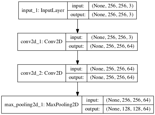
Plot of Convolutional Neural Network Architecture With a VGG Block
Using VGG blocks in your own models should be common because they are so simple and effective.
We can expand the example and demonstrate a single model that has three VGG blocks, the first two blocks have two convolutional layers with 64 and 128 filters respectively, the third block has four convolutional layers with 256 filters. This is a common usage of VGG blocks where the number of filters is increased with the depth of the model.
The complete code listing is provided below.
|
1 2 3 4 5 6 7 8 9 10 11 12 13 14 15 16 17 18 19 20 21 22 23 24 25 26 27 28 29 30 |
# Example of creating a CNN model with many VGG blocks from keras.models import Model from keras.layers import Input from keras.layers import Conv2D from keras.layers import MaxPooling2D from keras.utils import plot_model # function for creating a vgg block def vgg_block(layer_in, n_filters, n_conv): # add convolutional layers for _ in range(n_conv): layer_in = Conv2D(n_filters, (3,3), padding='same', activation='relu')(layer_in) # add max pooling layer layer_in = MaxPooling2D((2,2), strides=(2,2))(layer_in) return layer_in # define model input visible = Input(shape=(256, 256, 3)) # add vgg module layer = vgg_block(visible, 64, 2) # add vgg module layer = vgg_block(layer, 128, 2) # add vgg module layer = vgg_block(layer, 256, 4) # create model model = Model(inputs=visible, outputs=layer) # summarize model model.summary() # plot model architecture plot_model(model, show_shapes=True, to_file='multiple_vgg_blocks.png') |
Again, running the example summarizes the model architecture and we can clearly see the pattern of VGG blocks.
|
1 2 3 4 5 6 7 8 9 10 11 12 13 14 15 16 17 18 19 20 21 22 23 24 25 26 27 28 29 30 31 |
_________________________________________________________________ Layer (type) Output Shape Param # ================================================================= input_1 (InputLayer) (None, 256, 256, 3) 0 _________________________________________________________________ conv2d_1 (Conv2D) (None, 256, 256, 64) 1792 _________________________________________________________________ conv2d_2 (Conv2D) (None, 256, 256, 64) 36928 _________________________________________________________________ max_pooling2d_1 (MaxPooling2 (None, 128, 128, 64) 0 _________________________________________________________________ conv2d_3 (Conv2D) (None, 128, 128, 128) 73856 _________________________________________________________________ conv2d_4 (Conv2D) (None, 128, 128, 128) 147584 _________________________________________________________________ max_pooling2d_2 (MaxPooling2 (None, 64, 64, 128) 0 _________________________________________________________________ conv2d_5 (Conv2D) (None, 64, 64, 256) 295168 _________________________________________________________________ conv2d_6 (Conv2D) (None, 64, 64, 256) 590080 _________________________________________________________________ conv2d_7 (Conv2D) (None, 64, 64, 256) 590080 _________________________________________________________________ conv2d_8 (Conv2D) (None, 64, 64, 256) 590080 _________________________________________________________________ max_pooling2d_3 (MaxPooling2 (None, 32, 32, 256) 0 ================================================================= Total params: 2,325,568 Trainable params: 2,325,568 Non-trainable params: 0 _________________________________________________________________ |
A plot of the model architecture is created providing a different perspective on the same linear progression of layers.
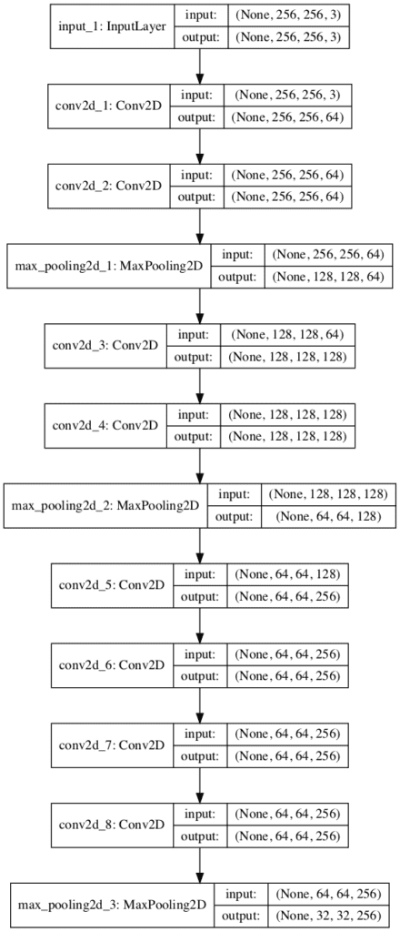
Plot of Convolutional Neural Network Architecture With Multiple VGG Blocks
How to Implement the Inception Module
The inception module was described and used in the GoogLeNet model in the 2015 paper by Christian Szegedy, et al. titled “Going Deeper with Convolutions.”
Like the VGG model, the GoogLeNet model achieved top results in the 2014 version of the ILSVRC challenge.
The key innovation on the inception model is called the inception module. This is a block of parallel convolutional layers with different sized filters (e.g. 1×1, 3×3, 5×5) and a and 3×3 max pooling layer, the results of which are then concatenated.
In order to avoid patch-alignment issues, current incarnations of the Inception architecture are restricted to filter sizes 1×1, 3×3 and 5×5; this decision was based more on convenience rather than necessity. […] Additionally, since pooling operations have been essential for the success of current convolutional networks, it suggests that adding an alternative parallel pooling path in each such stage should have additional beneficial effect, too
— Going Deeper with Convolutions, 2015.
This is a very simple and powerful architectural unit that allows the model to learn not only parallel filters of the same size, but parallel filters of differing sizes, allowing learning at multiple scales.
We can implement an inception module directly using the Keras functional API. The function below will create a single inception module with a fixed number of filters for each of the parallel convolutional layers. From the GoogLeNet architecture described in the paper, it does not appear to use a systematic sizing of filters for parallel convolutional layers as the model is highly optimized. As such, we can parameterize the module definition so that we can specify the number of filters to use in each of the 1×1, 3×3, and 5×5 filters.
|
1 2 3 4 5 6 7 8 9 10 11 12 13 |
# function for creating a naive inception block def inception_module(layer_in, f1, f2, f3): # 1x1 conv conv1 = Conv2D(f1, (1,1), padding='same', activation='relu')(layer_in) # 3x3 conv conv3 = Conv2D(f2, (3,3), padding='same', activation='relu')(layer_in) # 5x5 conv conv5 = Conv2D(f3, (5,5), padding='same', activation='relu')(layer_in) # 3x3 max pooling pool = MaxPooling2D((3,3), strides=(1,1), padding='same')(layer_in) # concatenate filters, assumes filters/channels last layer_out = concatenate([conv1, conv3, conv5, pool], axis=-1) return layer_out |
To use the function, provide the reference to the prior layer as input, the number of filters, and it will return a reference to the concatenated filters layer that you can then connect to more inception modules or a submodel for making a prediction.
We can demonstrate how to use this function by creating a model with a single inception module. In this case, the number of filters is based on “inception (3a)” from Table 1 in the paper.
The complete example is listed below.
|
1 2 3 4 5 6 7 8 9 10 11 12 13 14 15 16 17 18 19 20 21 22 23 24 25 26 27 28 29 30 31 32 |
# example of creating a CNN with an inception module from keras.models import Model from keras.layers import Input from keras.layers import Conv2D from keras.layers import MaxPooling2D from keras.layers.merge import concatenate from keras.utils import plot_model # function for creating a naive inception block def naive_inception_module(layer_in, f1, f2, f3): # 1x1 conv conv1 = Conv2D(f1, (1,1), padding='same', activation='relu')(layer_in) # 3x3 conv conv3 = Conv2D(f2, (3,3), padding='same', activation='relu')(layer_in) # 5x5 conv conv5 = Conv2D(f3, (5,5), padding='same', activation='relu')(layer_in) # 3x3 max pooling pool = MaxPooling2D((3,3), strides=(1,1), padding='same')(layer_in) # concatenate filters, assumes filters/channels last layer_out = concatenate([conv1, conv3, conv5, pool], axis=-1) return layer_out # define model input visible = Input(shape=(256, 256, 3)) # add inception module layer = naive_inception_module(visible, 64, 128, 32) # create model model = Model(inputs=visible, outputs=layer) # summarize model model.summary() # plot model architecture plot_model(model, show_shapes=True, to_file='naive_inception_module.png') |
Running the example creates the model and summarizes the layers.
We know the convolutional and pooling layers are parallel, but this summary does not capture the structure easily.
|
1 2 3 4 5 6 7 8 9 10 11 12 13 14 15 16 17 18 19 20 21 22 |
__________________________________________________________________________________________________ Layer (type) Output Shape Param # Connected to ================================================================================================== input_1 (InputLayer) (None, 256, 256, 3) 0 __________________________________________________________________________________________________ conv2d_1 (Conv2D) (None, 256, 256, 64) 256 input_1[0][0] __________________________________________________________________________________________________ conv2d_2 (Conv2D) (None, 256, 256, 128 3584 input_1[0][0] __________________________________________________________________________________________________ conv2d_3 (Conv2D) (None, 256, 256, 32) 2432 input_1[0][0] __________________________________________________________________________________________________ max_pooling2d_1 (MaxPooling2D) (None, 256, 256, 3) 0 input_1[0][0] __________________________________________________________________________________________________ concatenate_1 (Concatenate) (None, 256, 256, 227 0 conv2d_1[0][0] conv2d_2[0][0] conv2d_3[0][0] max_pooling2d_1[0][0] ================================================================================================== Total params: 6,272 Trainable params: 6,272 Non-trainable params: 0 __________________________________________________________________________________________________ |
A plot of the model architecture is also created that helps to clearly see the parallel structure of the module as well as the matching shapes of the output of each element of the module that allows their direct concatenation by the third dimension (filters or channels).
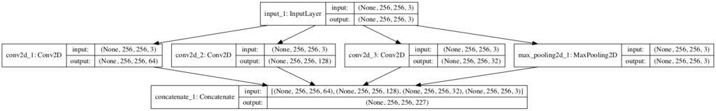
Plot of Convolutional Neural Network Architecture With a Naive Inception Module
The version of the inception module that we have implemented is called the naive inception module.
A modification to the module was made in order to reduce the amount of computation required. Specifically, 1×1 convolutional layers were added to reduce the number of filters before the 3×3 and 5×5 convolutional layers, and to increase the number of filters after the pooling layer.
This leads to the second idea of the Inception architecture: judiciously reducing dimension wherever the computational requirements would increase too much otherwise. […] That is, 1×1 convolutions are used to compute reductions before the expensive 3×3 and 5×5 convolutions. Besides being used as reductions, they also include the use of rectified linear activation making them dual-purpose
— Going Deeper with Convolutions, 2015.
If you intend to use many inception modules in your model, you may require this computational performance-based modification.
The function below implements this optimization improvement with parameterization so that you can control the amount of reduction in the number of filters prior to the 3×3 and 5×5 convolutional layers and the number of increased filters after max pooling.
|
1 2 3 4 5 6 7 8 9 10 11 12 13 14 15 16 |
# function for creating a projected inception module def inception_module(layer_in, f1, f2_in, f2_out, f3_in, f3_out, f4_out): # 1x1 conv conv1 = Conv2D(f1, (1,1), padding='same', activation='relu')(layer_in) # 3x3 conv conv3 = Conv2D(f2_in, (1,1), padding='same', activation='relu')(layer_in) conv3 = Conv2D(f2_out, (3,3), padding='same', activation='relu')(conv3) # 5x5 conv conv5 = Conv2D(f3_in, (1,1), padding='same', activation='relu')(layer_in) conv5 = Conv2D(f3_out, (5,5), padding='same', activation='relu')(conv5) # 3x3 max pooling pool = MaxPooling2D((3,3), strides=(1,1), padding='same')(layer_in) pool = Conv2D(f4_out, (1,1), padding='same', activation='relu')(pool) # concatenate filters, assumes filters/channels last layer_out = concatenate([conv1, conv3, conv5, pool], axis=-1) return layer_out |
We can create a model with two of these optimized inception modules to get a concrete idea of how the architecture looks in practice.
In this case, the number of filter configurations are based on “inception (3a)” and “inception (3b)” from Table 1 in the paper.
The complete example is listed below.
|
1 2 3 4 5 6 7 8 9 10 11 12 13 14 15 16 17 18 19 20 21 22 23 24 25 26 27 28 29 30 31 32 33 34 35 36 37 |
# example of creating a CNN with an efficient inception module from keras.models import Model from keras.layers import Input from keras.layers import Conv2D from keras.layers import MaxPooling2D from keras.layers.merge import concatenate from keras.utils import plot_model # function for creating a projected inception module def inception_module(layer_in, f1, f2_in, f2_out, f3_in, f3_out, f4_out): # 1x1 conv conv1 = Conv2D(f1, (1,1), padding='same', activation='relu')(layer_in) # 3x3 conv conv3 = Conv2D(f2_in, (1,1), padding='same', activation='relu')(layer_in) conv3 = Conv2D(f2_out, (3,3), padding='same', activation='relu')(conv3) # 5x5 conv conv5 = Conv2D(f3_in, (1,1), padding='same', activation='relu')(layer_in) conv5 = Conv2D(f3_out, (5,5), padding='same', activation='relu')(conv5) # 3x3 max pooling pool = MaxPooling2D((3,3), strides=(1,1), padding='same')(layer_in) pool = Conv2D(f4_out, (1,1), padding='same', activation='relu')(pool) # concatenate filters, assumes filters/channels last layer_out = concatenate([conv1, conv3, conv5, pool], axis=-1) return layer_out # define model input visible = Input(shape=(256, 256, 3)) # add inception block 1 layer = inception_module(visible, 64, 96, 128, 16, 32, 32) # add inception block 1 layer = inception_module(layer, 128, 128, 192, 32, 96, 64) # create model model = Model(inputs=visible, outputs=layer) # summarize model model.summary() # plot model architecture plot_model(model, show_shapes=True, to_file='inception_module.png') |
Running the example creates a linear summary of the layers that does not really help to understand what is going on.
|
1 2 3 4 5 6 7 8 9 10 11 12 13 14 15 16 17 18 19 20 21 22 23 24 25 26 27 28 29 30 31 32 33 34 35 36 37 38 39 40 41 42 43 44 45 46 47 |
__________________________________________________________________________________________________ Layer (type) Output Shape Param # Connected to ================================================================================================== input_1 (InputLayer) (None, 256, 256, 3) 0 __________________________________________________________________________________________________ conv2d_2 (Conv2D) (None, 256, 256, 96) 384 input_1[0][0] __________________________________________________________________________________________________ conv2d_4 (Conv2D) (None, 256, 256, 16) 64 input_1[0][0] __________________________________________________________________________________________________ max_pooling2d_1 (MaxPooling2D) (None, 256, 256, 3) 0 input_1[0][0] __________________________________________________________________________________________________ conv2d_1 (Conv2D) (None, 256, 256, 64) 256 input_1[0][0] __________________________________________________________________________________________________ conv2d_3 (Conv2D) (None, 256, 256, 128 110720 conv2d_2[0][0] __________________________________________________________________________________________________ conv2d_5 (Conv2D) (None, 256, 256, 32) 12832 conv2d_4[0][0] __________________________________________________________________________________________________ conv2d_6 (Conv2D) (None, 256, 256, 32) 128 max_pooling2d_1[0][0] __________________________________________________________________________________________________ concatenate_1 (Concatenate) (None, 256, 256, 256 0 conv2d_1[0][0] conv2d_3[0][0] conv2d_5[0][0] conv2d_6[0][0] __________________________________________________________________________________________________ conv2d_8 (Conv2D) (None, 256, 256, 128 32896 concatenate_1[0][0] __________________________________________________________________________________________________ conv2d_10 (Conv2D) (None, 256, 256, 32) 8224 concatenate_1[0][0] __________________________________________________________________________________________________ max_pooling2d_2 (MaxPooling2D) (None, 256, 256, 256 0 concatenate_1[0][0] __________________________________________________________________________________________________ conv2d_7 (Conv2D) (None, 256, 256, 128 32896 concatenate_1[0][0] __________________________________________________________________________________________________ conv2d_9 (Conv2D) (None, 256, 256, 192 221376 conv2d_8[0][0] __________________________________________________________________________________________________ conv2d_11 (Conv2D) (None, 256, 256, 96) 76896 conv2d_10[0][0] __________________________________________________________________________________________________ conv2d_12 (Conv2D) (None, 256, 256, 64) 16448 max_pooling2d_2[0][0] __________________________________________________________________________________________________ concatenate_2 (Concatenate) (None, 256, 256, 480 0 conv2d_7[0][0] conv2d_9[0][0] conv2d_11[0][0] conv2d_12[0][0] ================================================================================================== Total params: 513,120 Trainable params: 513,120 Non-trainable params: 0 __________________________________________________________________________________________________ |
A plot of the model architecture is created that does make the layout of each module clear and how the first model feeds the second module.
Note that the first 1×1 convolution in each inception module is on the far right for space reasons, but besides that, the other layers are organized left to right within each module.
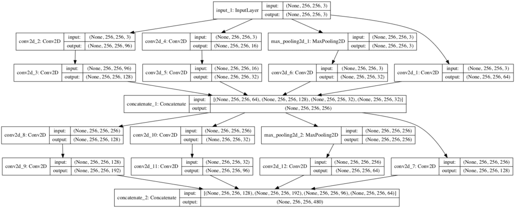
Plot of Convolutional Neural Network Architecture With a Efficient Inception Module
How to Implement the Residual Module
The Residual Network, or ResNet, architecture for convolutional neural networks was proposed by Kaiming He, et al. in their 2016 paper titled “Deep Residual Learning for Image Recognition,” which achieved success on the 2015 version of the ILSVRC challenge.
A key innovation in the ResNet was the residual module. The residual module, specifically the identity residual model, is a block of two convolutional layers with the same number of filters and a small filter size where the output of the second layer is added with the input to the first convolutional layer. Drawn as a graph, the input to the module is added to the output of the module and is called a shortcut connection.
We can implement this directly in Keras using the functional API and the add() merge function.
|
1 2 3 4 5 6 7 8 9 10 11 |
# function for creating an identity residual module def residual_module(layer_in, n_filters): # conv1 conv1 = Conv2D(n_filters, (3,3), padding='same', activation='relu', kernel_initializer='he_normal')(layer_in) # conv2 conv2 = Conv2D(n_filters, (3,3), padding='same', activation='linear', kernel_initializer='he_normal')(conv1) # add filters, assumes filters/channels last layer_out = add([conv2, layer_in]) # activation function layer_out = Activation('relu')(layer_out) return layer_out |
A limitation with this direct implementation is that if the number of filters in the input layer does not match the number of filters in the last convolutional layer of the module (defined by n_filters), then we will get an error.
One solution is to use a 1×1 convolution layer, often referred to as a projection layer, to either increase the number of filters for the input layer or reduce the number of filters for the last convolutional layer in the module. The former solution makes more sense, and is the approach proposed in the paper, referred to as a projection shortcut.
When the dimensions increase […], we consider two options: (A) The shortcut still performs identity mapping, with extra zero entries padded for increasing dimensions. This option introduces no extra parameter; (B) The projection shortcut […] is used to match dimensions (done by 1×1 convolutions).
— Deep Residual Learning for Image Recognition, 2015.
Below is an updated version of the function that will use the identity if possible, otherwise a projection of the number of filters in the input does not match the n_filters argument.
|
1 2 3 4 5 6 7 8 9 10 11 12 13 14 15 |
# function for creating an identity or projection residual module def residual_module(layer_in, n_filters): merge_input = layer_in # check if the number of filters needs to be increase, assumes channels last format if layer_in.shape[-1] != n_filters: merge_input = Conv2D(n_filters, (1,1), padding='same', activation='relu', kernel_initializer='he_normal')(layer_in) # conv1 conv1 = Conv2D(n_filters, (3,3), padding='same', activation='relu', kernel_initializer='he_normal')(layer_in) # conv2 conv2 = Conv2D(n_filters, (3,3), padding='same', activation='linear', kernel_initializer='he_normal')(conv1) # add filters, assumes filters/channels last layer_out = add([conv2, merge_input]) # activation function layer_out = Activation('relu')(layer_out) return layer_out |
We can demonstrate the usage of this module in a simple model.
The complete example is listed below.
|
1 2 3 4 5 6 7 8 9 10 11 12 13 14 15 16 17 18 19 20 21 22 23 24 25 26 27 28 29 30 31 32 33 34 35 |
# example of a CNN model with an identity or projection residual module from keras.models import Model from keras.layers import Input from keras.layers import Activation from keras.layers import Conv2D from keras.layers import MaxPooling2D from keras.layers import add from keras.utils import plot_model # function for creating an identity or projection residual module def residual_module(layer_in, n_filters): merge_input = layer_in # check if the number of filters needs to be increase, assumes channels last format if layer_in.shape[-1] != n_filters: merge_input = Conv2D(n_filters, (1,1), padding='same', activation='relu', kernel_initializer='he_normal')(layer_in) # conv1 conv1 = Conv2D(n_filters, (3,3), padding='same', activation='relu', kernel_initializer='he_normal')(layer_in) # conv2 conv2 = Conv2D(n_filters, (3,3), padding='same', activation='linear', kernel_initializer='he_normal')(conv1) # add filters, assumes filters/channels last layer_out = add([conv2, merge_input]) # activation function layer_out = Activation('relu')(layer_out) return layer_out # define model input visible = Input(shape=(256, 256, 3)) # add vgg module layer = residual_module(visible, 64) # create model model = Model(inputs=visible, outputs=layer) # summarize model model.summary() # plot model architecture plot_model(model, show_shapes=True, to_file='residual_module.png') |
Running the example first creates the model then prints a summary of the layers.
Because the module is linear, this summary is helpful to see what is going on.
|
1 2 3 4 5 6 7 8 9 10 11 12 13 14 15 16 17 18 19 20 |
__________________________________________________________________________________________________ Layer (type) Output Shape Param # Connected to ================================================================================================== input_1 (InputLayer) (None, 256, 256, 3) 0 __________________________________________________________________________________________________ conv2d_2 (Conv2D) (None, 256, 256, 64) 1792 input_1[0][0] __________________________________________________________________________________________________ conv2d_3 (Conv2D) (None, 256, 256, 64) 36928 conv2d_2[0][0] __________________________________________________________________________________________________ conv2d_1 (Conv2D) (None, 256, 256, 64) 256 input_1[0][0] __________________________________________________________________________________________________ add_1 (Add) (None, 256, 256, 64) 0 conv2d_3[0][0] conv2d_1[0][0] __________________________________________________________________________________________________ activation_1 (Activation) (None, 256, 256, 64) 0 add_1[0][0] ================================================================================================== Total params: 38,976 Trainable params: 38,976 Non-trainable params: 0 __________________________________________________________________________________________________ |
A plot of the model architecture is also created.
We can see the module with the inflation of the number of filters in the input and the addition of the two elements at the end of the module.
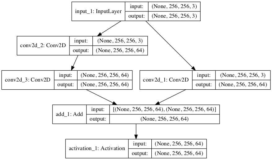
Plot of Convolutional Neural Network Architecture With an Residual Module
The paper describes other types of residual connections such as bottlenecks. These are left as an exercise for the reader that can be implemented easily by updating the residual_module() function.
Further Reading
This section provides more resources on the topic if you are looking to go deeper.
Posts
Papers
- Gradient-based learning applied to document recognition, (PDF) 1998.
- ImageNet Classification with Deep Convolutional Neural Networks, 2012.
- Very Deep Convolutional Networks for Large-Scale Image Recognition, 2014.
- Going Deeper with Convolutions, 2015.
- Deep Residual Learning for Image Recognition, 2016
API
Summary
In this tutorial, you discovered how to implement key architecture elements from milestone convolutional neural network models, from scratch.
Specifically, you learned:
- How to implement a VGG module used in the VGG-16 and VGG-19 convolutional neural network models.
- How to implement the naive and optimized inception module used in the GoogLeNet model.
- How to implement the identity residual module used in the ResNet model.
Do you have any questions?
Ask your questions in the comments below and I will do my best to answer.
Develop Deep Learning Models for Vision Today!

Develop Your Own Vision Models in Minutes
...with just a few lines of python code
Discover how in my new Ebook:
Deep Learning for Computer Vision
It provides self-study tutorials on topics like:
classification, object detection (yolo and rcnn), face recognition (vggface and facenet), data preparation and much more...
Finally Bring Deep Learning to your Vision Projects
Skip the Academics. Just Results.
 for Evaluating GANs")
 for Evaluating GANs")


 From Scratch with Keras")

I love your code-snippets and practical examples on implementation. These are exactly the time-savers and error-avoiders that a beginner needs to get experimenting. Thanks a lot. I’m still struggling a bit with the concept of the 1×1 convolution filters, though. A post on that topic alone – but in more detail on what the layer actually does and how it works – would be very helpful. (I will need to re-read and try this post here a few times, I guess. Comment written after first read-through.)
Thanks.
I hope to have a post dedicated to the topic soon.
Thank you for your effort. I learn a lot from you.
You’re welcome.
Thanks Jason,
Your blogs and the explanations are always very useful and distilled.Your books are equally excellent.
I have a lot of interest in combination of CNN and LSTM having read all your blogs, purchased time series and the latest book, particularly in handling temporal sequential problems concerning acquiring images from a plant for the diagnosis of disease development over time.
Would appreciate if a blog on combination of this two models is done for clarity with a unique example.Your advice is more than welcome.
Thanks for the suggestion.
I believe there is an example of processing images over time in the LSTM book. I hope to cover more examples in the future.
I suppose that in the last section there is an error , when using merge_input the conv1 must be attached not to layer_in but to the merge_input , wasn’t it ?
I don’t believe there’s an error.
Which example are you referring to exactly?
The last code in the 17th line .
You’re right, thanks! Fixed.
Update, no, that is not an error.
The 1×1 projection is only needed of the number of channels for the input does not match the number of channels in the output.
Hi Jason! This is a great tutorial on VGG and inception. Thank you for that. I have a question, though. This way you developed your codes in this tutorial is kind of new to me. In your previous posts, you use sequential models and then you use ‘model.add’. Is this a specific way to develop VGG or we can still use that format (e.g. ‘model.add’) to develop these architectures? Thank you in advance!
Yes, here we are using the functional API, you can learn more about it here:
https://machinelearningmastery.com/keras-functional-api-deep-learning/
Oh, thank you! You are the best, Jason!
No problem.
Thanks Jason for another great tutorial as always!
Many models from Keras application requires 224×224 images.
Is there a way to use bigger image with the pre-trained models without resizing?
If not, is there a way to at least use their architectures without their weights, and train from scratch?
Thanks!
Yes, you can specific a new input layer with your preferred size.
This might help:
https://machinelearningmastery.com/how-to-use-transfer-learning-when-developing-convolutional-neural-network-models/
Wow, very simple! “input_tensor=new_input” Thanks! By the way, am I supposed to get an email notification if I get a reply to my comment?
Yes, very simple.
No, I don’t have email notifications on the blog comments – at least not at this stage.
Amazing Tutorials!!!
Thanks.
Hi Jason,
We added 1×1 convolutional layer prior to 3×3 and 5×5 layers in the projected inception module in order to reduce the amount of computation. We can, however, easily see that for example the number of parameters has increased to 110720 from 3584 for 128 filters of size 3×3 in the naive inception module. I wonder why it increased while we intended to reduce it! And would you mind if you give me a hint about how it calculates the number of parameters? Much obligied!
Nice observation. We are trading off space complexity for time complexity. E.g. less compute but more weights.
Thank you! But I guess this way we’re putting the burden on memory rather than on GPU. Like I got OOM when I wanted to use this module for sequential data i.e. replacing CONV2D by CONVLSTM2D because I got >500M parameters! While with VGA I got 40M which was calculable by my RAM (16Gb)
And I don’t know why but for some reasons when I used only one block, the number of parameters became negative!!
That is surprising!
Your stuff is very helpful for the newcomers. Thank you!!
Thanks, I’m happy to hear that.
Jason I really love your tutorials. If I want to use the above models for single class object detection how can I do that.
Thanks!
Perhaps start with this:
https://machinelearningmastery.com/how-to-train-an-object-detection-model-with-keras/
Jason, in the above mentioned link you have used a predefined mrcnn model. I wanted to know how a deep learning modules (like SSD, VGG, Inception and Resent) is used in object detection. I understood how an above mentioned models are used as a classifiers, but I confuse when I tried to use the same models for object detection.
What is the major difference between SSD based image classifier and SSD based object detection.
Your help is highly appreciated.
Object detection and image classification are very different problems, and use different models.
E.g. Mask RCNN and YOLO are used for object detection. VGG is used for image classification.
This post will help with the differences:
https://machinelearningmastery.com/object-recognition-with-deep-learning/
Janson,
Thank you for the fast reply. I have gone through the suggested material. In that blog you have mentioned VGG-16 as a feature extractor model for object detection. I am interested to know a little more information about the object detection architecture.
I have tutorials on rcnn and yolo if you want to learn more about them. Beyond that, you can dive into the papers on those topics.
Hi Jason,
Thank you for this impressive article.
I am trying to implement naive inception modul but i have error “ValueError: Error when checking target: expected concatenate_2 to have 4 dimensions, but got array with shape (2, 5)” If you do not mind could you help me to understand what is it about? specifically about “shape (2,5)”. For your information I plug and play the naive inception modul as your explanation.
Thank you very much.
Sorry to hear that.
Perhaps start with the simple example in the blog post, get that working first, then slowly adapt it for your needs?
Thank your post about CNN archictectures,
I am trying your “projected inception module” with my dataset, then add:
x = Flatten()(layer)
x =(Dense(128, activation=’sigmoid’))(x)
x = (Dense(15, activation=’softmax’))(x)
model = Model(inputs=visible, outputs=x, name=’Simple_inception_v3′)
model.compile(loss=’categorical_crossentropy’, optimizer=’adam’, metrics=[‘accuracy’])
Unfortunatly, I get the same acc and loss all epochs.
Epoch 1/10
1811675/1811675 [=========] – 516s 285us/step – loss: 0.7715 – accuracy: 0.8030 – val_loss: 0.7724 – val_accuracy: 0.8027
Epoch 2/10
1811675/1811675 [=========] – 512s 282us/step – loss: 0.7713 – accuracy: 0.8031 – val_loss: 0.7691 – val_accuracy: 0.8027
Epoch 3/10
1811675/1811675 [=========] – 480s 265us/step – loss: 0.7712 – accuracy: 0.8031 – val_loss: 0.7706 – val_accuracy: 0.8027
Epoch 4/10
1811675/1811675 [=========] – 477s 263us/step – loss: 0.7712 – accuracy: 0.8031 – val_loss: 0.7711 – val_accuracy: 0.8027
Epoch 10/10
1811675/1811675 [=========] – 508s 280us/step – loss: 0.7713 – accuracy: 0.8031 – val_loss: 0.7720 – val_accuracy: 0.8027
Can you give me some points to improve my model
Thank you very much
Well done.
Yes, the general suggestions here will help you improve the performance of your model:
https://machinelearningmastery.com/start-here/#better
hello, thank you for your efforts, i am a beginner in machine learning and i have a project with monocular depth from single image with kitti dataset could you please guide me how to start the code .thank you in advance
Perhaps start with the tutorials here to get familiar with this type of project:
https://machinelearningmastery.com/start-here/#dlfcv
what kind of resnet is in that exampled?? thanks
The paper is cited and linked directly.
Hi Jason!
In the ResNet module, you have chosen to use linear activation. May I know the reason why you chose this particular activation? And in case, we wish to Batch Norm, would you prefer using it before t
The example implements the resnset block as defined in the paper.
Hi Jason,
Thank you so much for your nice explanation.
I have a question regarding backpropagation in ResNet architecture. Does the BP updates the parameters via short-cut connections, however there are no parameters to learn?, and same question implies in addition process, becasue if we see summary of the model, add layer also has nothing to learn. So, my question is that how backpropagation is performed to the lower layers? I am bit confused at this point. It would be a great help.
Thank you!
You’re welcome.
Yes, backprop flows over all connections when propagating error back through the net.
Hi Jason.
For Resnet, we know that skip connection help network to learn Indentity(in the main branch).
But how to prove that that certain block of resnet already learn the indentity? any idea?
Thanks
Mike
Not offhand, perhaps you can experiment with small modifications and compare the results.
Thank you very much your tutorials , i used to read your tutorials , i would ask do you have more implementation (examples ) in inception and Resnet? I read there are inception3 and inception4 and i don’t find implementation in you website .
I don’t think so.
Nice introduction about how to implement different models. I am a beginner at deep learning concepts. I was working on forgery images(copy-move/Image splicing). I wanted to find the exact regions of an image where the copy-pasted regions are present in an image. Sir, can you suggest keeping learning concepts to identify forgery regions present in images.
Perhaps you can explore the problem as an object detection type problem, e.g. train a model to locate these edited regions on a dataset you have prepared.
Hi. Thanks for your work.
I have a question – I didn’t found an answer in the ResNet paper. On shortcut conv layer you have activation=’relu’
if layer_in.shape[-1] != n_filters:
merge_input = Conv2D(n_filters, (1,1), padding=’same’, activation=’relu’ …
should that activation be linear ?
It is always linear before layer ADD in Inception-V4 paper
https://arxiv.org/pdf/1602.07261.pdf
Great!
I don’t think so.
Hi Jason,
is there any way to use Keras Applications (like VGG, Resnet, and Inception) for non-image-like data? All examples above required image-like data with shapes like (256, 256,3). For instance, I have temporal data like sound with shape (300,1). I can extract a spectrogram of sound which has an image-like data shape, but I want to avoid it since it is time-consuming. I want to directly input temporal features to architecture like VGG of ResNet.
It would not really make sense given the layers have learned features for image data.
Dear Jason
I would like to use ResNet defined model to my (340,340,1) 3 class classification.
Tensors include data points, they are not images.
I made these changes in definition:
visible = Input(shape=(340, 340, 1))
Then I am using:
model.compile(loss=’categorical_crossentropy’, optimizer=’Adam’, metrics = [‘accuracy’])
model.fit(X_train, y_train, batch_size = 4, epochs = 2, validation_data=(X_test, y_test),callbacks=[callback])
results = model.evaluate(X_test, y_test)
I am using one hot encoding for labeling.
I received this error:
ValueError: Shapes (None, 3) and (None, 340, 340, 64) are incompatible
What do you recommend to solve this problem?
Best.
Hi Mesut…Are you implementing a CNN model?