Pooling can be used to down sample the content of feature maps, reducing their width and height whilst maintaining their salient features.
A problem with deep convolutional neural networks is that the number of feature maps often increases with the depth of the network. This problem can result in a dramatic increase in the number of parameters and computation required when larger filter sizes are used, such as 5×5 and 7×7.
To address this problem, a 1×1 convolutional layer can be used that offers a channel-wise pooling, often called feature map pooling or a projection layer. This simple technique can be used for dimensionality reduction, decreasing the number of feature maps whilst retaining their salient features. It can also be used directly to create a one-to-one projection of the feature maps to pool features across channels or to increase the number of feature maps, such as after traditional pooling layers.
In this tutorial, you will discover how to use 1×1 filters to control the number of feature maps in a convolutional neural network.
After completing this tutorial, you will know:
The 1×1 filter can be used to create a linear projection of a stack of feature maps.
The projection created by a 1×1 can act like channel-wise pooling and be used for dimensionality reduction.
The projection created by a 1×1 can also be used directly or be used to increase the number of feature maps in a model.
Kick-start your project with my new book Deep Learning for Computer Vision, including step-by-step tutorials and the Python source code files for all examples.
Let’s get started.
A Gentle Introduction to 1×1 Convolutions to Reduce the Complexity of Convolutional Neural Networks Photo copyright, some rights reserved.
Tutorial Overview
This tutorial is divided into five parts; they are:
Convolutions Over Channels
Problem of Too Many Feature Maps
Downsample Feature Maps With 1×1 Filters
Examples of How to Use 1×1 Convolutions
Examples of 1×1 Filters in CNN Model Architectures
Convolutions Over Channels
Recall that a convolutional operation is a linear application of a smaller filter to a larger input that results in an output feature map.
A filter applied to an input image or input feature map always results in a single number. The systematic left-to-right and top-to-bottom application of the filter to the input results in a two-dimensional feature map. One filter creates one corresponding feature map.
A filter must have the same depth or number of channels as the input, yet, regardless of the depth of the input and the filter, the resulting output is a single number and one filter creates a feature map with a single channel.
Let’s make this concrete with some examples:
If the input has one channel such as a grayscale image, then a 3×3 filter will be applied in 3x3x1 blocks.
If the input image has three channels for red, green, and blue, then a 3×3 filter will be applied in 3x3x3 blocks.
If the input is a block of feature maps from another convolutional or pooling layer and has the depth of 64, then the 3×3 filter will be applied in 3x3x64 blocks to create the single values to make up the single output feature map.
The depth of the output of one convolutional layer is only defined by the number of parallel filters applied to the input.
Want Results with Deep Learning for Computer Vision?
Take my free 7-day email crash course now (with sample code).
Click to sign-up and also get a free PDF Ebook version of the course.
Problem of Too Many Feature Maps
The depth of the input or number of filters used in convolutional layers often increases with the depth of the network, resulting in an increase in the number of resulting feature maps. It is a common model design pattern.
Further, some network architectures, such as the inception architecture, may also concatenate the output feature maps from multiple convolutional layers, which may also dramatically increase the depth of the input to subsequent convolutional layers.
A large number of feature maps in a convolutional neural network can cause a problem as a convolutional operation must be performed down through the depth of the input. This is a particular problem if the convolutional operation being performed is relatively large, such as 5×5 or 7×7 pixels, as it can result in considerably more parameters (weights) and, in turn, computation to perform the convolutional operations (large space and time complexity).
Pooling layers are designed to downscale feature maps and systematically halve the width and height of feature maps in the network. Nevertheless, pooling layers do not change the number of filters in the model, the depth, or number of channels.
Deep convolutional neural networks require a corresponding pooling type of layer that can downsample or reduce the depth or number of feature maps.
Downsample Feature Maps With 1×1 Filters
The solution is to use a 1×1 filter to down sample the depth or number of feature maps.
A 1×1 filter will only have a single parameter or weight for each channel in the input, and like the application of any filter results in a single output value. This structure allows the 1×1 filter to act like a single neuron with an input from the same position across each of the feature maps in the input. This single neuron can then be applied systematically with a stride of one, left-to-right and top-to-bottom without any need for padding, resulting in a feature map with the same width and height as the input.
The 1×1 filter is so simple that it does not involve any neighboring pixels in the input; it may not be considered a convolutional operation. Instead, it is a linear weighting or projection of the input. Further, a nonlinearity is used as with other convolutional layers, allowing the projection to perform non-trivial computation on the input feature maps.
This simple 1×1 filter provides a way to usefully summarize the input feature maps. The use of multiple 1×1 filters, in turn, allows the tuning of the number of summaries of the input feature maps to create, effectively allowing the depth of the feature maps to be increased or decreased as needed.
A convolutional layer with a 1×1 filter can, therefore, be used at any point in a convolutional neural network to control the number of feature maps. As such, it is often referred to as a projection operation or projection layer, or even a feature map or channel pooling layer.
Now that we know that we can control the number of feature maps with 1×1 filters, let’s make it concrete with some examples.
Examples of How to Use 1×1 Convolutions
We can make the use of a 1×1 filter concrete with some examples.
Consider that we have a convolutional neural network that expected color images input with the square shape of 256x256x3 pixels.
These images then pass through a first hidden layer with 512 filters, each with the size of 3×3 with the same padding, followed by a ReLU activation function.
A 1×1 filter can be used to create a projection of the feature maps.
The number of feature maps created will be the same number and the effect may be a refinement of the features already extracted. This is often called channel-wise pooling, as opposed to traditional feature-wise pooling on each channel. It can be implemented as follows:
1
model.add(Conv2D(512,(1,1),activation='relu'))
We can see that we use the same number of features and still follow the application of the filter with a rectified linear activation function.
Running the example creates the model and summarizes the architecture.
We can see that no change is made to the width or height of the feature maps, and by design, the number of feature maps is kept constant with a simple projection operation applied.
The 1×1 filter can be used to decrease the number of feature maps.
This is the most common application of this type of filter and in this way, the layer is often called a feature map pooling layer.
In this example, we can decrease the depth (or channels) from 512 to 64. This might be useful if the subsequent layer we were going to add to our model would be another convolutional layer with 7×7 filters. These filters would only be applied at a depth of 64 rather than 512.
1
model.add(Conv2D(64,(1,1),activation='relu'))
The composition of the 64 feature maps is not the same as the original 512, but contains a useful summary of dimensionality reduction that captures the salient features, such that the 7×7 operation may have a similar effect on the 64 feature maps as it might have on the original 512.
Further, a 7×7 convolutional layer with 64 filters itself applied to the 512 feature maps output by the first hidden layer would result in approximately one million parameters (weights). If the 1×1 filter is used to reduce the number of feature maps to 64 first, then the number of parameters required for the 7×7 layer is only approximately 200,000, an enormous difference.
The complete example of using a 1×1 filter for dimensionality reduction is listed below.
1
2
3
4
5
6
7
8
9
# example of a 1x1 filter for dimensionality reduction
The 1×1 filter can be used to increase the number of feature maps.
This is a common operation used after a pooling layer prior to applying another convolutional layer.
The projection effect of the filter can be applied as many times as needed to the input, allowing the number of feature maps to be scaled up and yet have a composition that captures the salient features of the original.
We can increase the number of feature maps from 512 input from the first hidden layer to double the size at 1,024 feature maps.
1
model.add(Conv2D(1024,(1,1),activation='relu'))
The complete example is listed below.
1
2
3
4
5
6
7
8
9
# example of a 1x1 filter to increase dimensionality
Running the example creates the model and summarizes its structure.
We can see that the width and height of the feature maps are unchanged and that the number of feature maps was increased from 512 to double the size at 1,024.
Now that we are familiar with how to use 1×1 filters, let’s look at some examples where they have been used in the architecture of convolutional neural network models.
Examples of 1×1 Filters in CNN Model Architectures
In this section, we will highlight some important examples where 1×1 filters have been used as key elements in modern convolutional neural network model architectures.
Network in Network
The 1×1 filter was perhaps first described and popularized in the 2013 paper by Min Lin, et al. in their paper titled “Network In Network.”
In the paper, the authors propose the need for an MLP convolutional layer and the need for cross-channel pooling to promote learning across channels.
This cascaded cross channel parametric pooling structure allows complex and learnable interactions of cross channel information.
They describe a 1×1 convolutional layer as a specific implementation of cross-channel parametric pooling, which, in effect, that is exactly what a 1×1 filter achieves.
Each pooling layer performs weighted linear recombination on the input feature maps, which then go through a rectifier linear unit. […] The cross channel parametric pooling layer is also equivalent to a convolution layer with 1×1 convolution kernel.
The 1×1 filter was used explicitly for dimensionality reduction and for increasing the dimensionality of feature maps after pooling in the design of the inception module, used in the GoogLeNet model by Christian Szegedy, et al. in their 2014 paper titled “Going Deeper with Convolutions.”
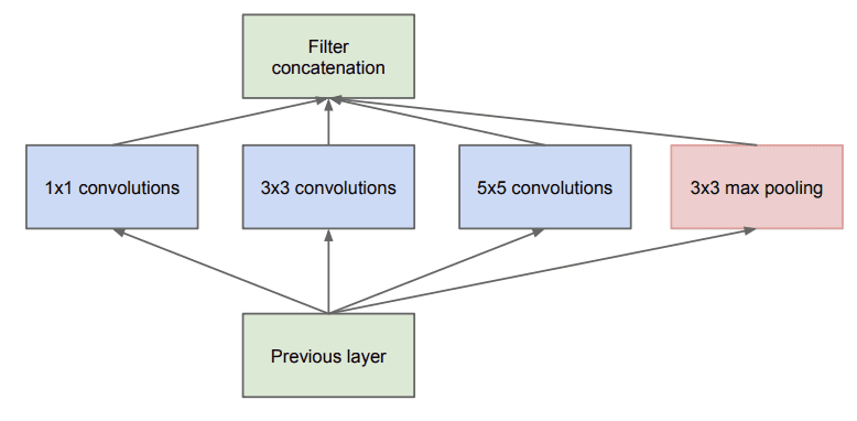
The paper describes an “inception module” where an input block of feature maps is processed in parallel by different convolutional layers each with differently sized filters, where a 1×1 size filter is one of the layers used.
Example of the Naive Inception Module Taken from Going Deeper with Convolutions, 2014.
The output of the parallel layers are then stacked, channel-wise, resulting in very deep stacks of convolutional layers to be processed by subsequent inception modules.
The merging of the output of the pooling layer with the outputs of convolutional layers would lead to an inevitable increase in the number of outputs from stage to stage. Even while this architecture might cover the optimal sparse structure, it would do it very inefficiently, leading to a computational blow up within a few stages.
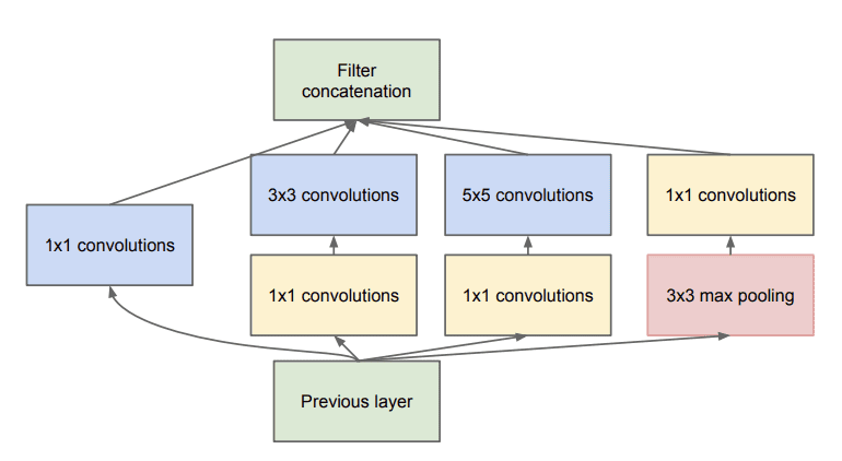
The inception module is then redesigned to use 1×1 filters to reduce the number of feature maps prior to parallel convolutional layers with 5×5 and 7×7 sized filters.
This leads to the second idea of the proposed architecture: judiciously applying dimension reductions and projections wherever the computational requirements would increase too much otherwise. […] That is, 1×1 convolutions are used to compute reductions before the expensive 3×3 and 5×5 convolutions. Besides being used as reductions, they also include the use of rectified linear activation which makes them dual-purpose
The 1×1 filter is also used to increase the number of feature maps after pooling, artificially creating more projections of the downsampled feature map content.
Example of the Inception Module With Dimensionality Reduction Taken from Going Deeper with Convolutions, 2014.
Residual Architecture
The 1×1 filter was used as a projection technique to match the number of filters of input to the output of residual modules in the design of the residual network by Kaiming He, et al. in their 2015 paper titled “Deep Residual Learning for Image Recognition.”
The authors describe an architecture comprised of “residual modules” where the input to a module is added to the output of the module in what is referred to as a shortcut connection.
Because the input is added to the output of the module, the dimensionality must match in terms of width, height, and depth. Width and height can be maintained via padding, although a 1×1 filter is used to change the depth of the input as needed so that it can be added with the output of the module. This type of connection is referred to as a projection shortcut connection.
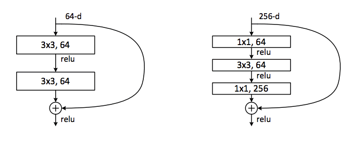
Further, the residual modules use a bottleneck design with 1×1 filters to reduce the number of feature maps for computational efficiency reasons.
The three layers are 1×1, 3×3, and 1×1 convolutions, where the 1×1 layers are responsible for reducing and then increasing (restoring) dimensions, leaving the 3×3 layer a bottleneck with smaller input/output dimensions.
It provides self-study tutorials on topics like: classification, object detection (yolo and rcnn), face recognition (vggface and facenet), data preparation and much more...
Finally Bring Deep Learning to your Vision Projects
dear jason, what do you mean by
1- single parameter or weight for each channel in the input.
2- act like a single neuron with an input from the same position across each of the feature maps.
thank you for your nice article.
Would you like to share your work with pytorch version.
Pytorh is popular and if you can add a version of your code written by pytorch, we will appreciate you very much.
I’m wondering what is the difference between a Conv2D(512, (1,1), activation=’relu’) layer and a Dense(512, activation=’relu’) layer? I’m a beginner (a few months of NN experience) and probably missing something, but from my perspective, a Conv2D layer with kernel_size=(1,1) is equivalent to a weight in a Dense layer, and both Dense layers and Conv2D layers have bias, so is there another difference that I am missing? Or is there a benefit to Conv2D with kernel_size=(1,1) instead of Dense?
Thanks in advance, this article was super helpful!
Practically, I think there may be a difference in how the inputs are processed, e.g. conv does a good job of reduction channels, not sure dense would do the same thing.
Analysis is required to give a helpful/real answer.
Thanks! I’m training some models to do some real-world analysis on it, and it seems to give comparable results, but I just wanted to check that those results weren’t specific to my applications.
In regards to 1×1 convolution, you have made this statement “These filters would only be applied at a depth of 64 rather than 512” but as per Andrew Ng these each filter is of size 1x1x previous channel size so it will be 1x1x512 for a single filter- if you need to reduce the channel from 512 to 64, itcan be reduced only by adding 64 such filters. Your statement and his are contradicting.
Not sure if this is obvious thing to everyone, at least not for me. In the first simple example you said that “the output of the first hidden layer is … 256x256x512.” I was wondering that how to calculate the total number of parameters 14336 in the model, that is shown in the summary. You can probably get it by calculating 3x3x3x512+512=14336.
Maybe you’ve covered this issue in another tutorial?
There are standard calculations for the number of weights and number of outputs based on the specified model architecture. Sorry, I don’t have a tutorial on the topic – at least I don’t think I do.
i dont quite follow about “decreasing feature maps” with 1×1 conv.
In your example, a 512 filters 3×3 conv2d followed by a 64 filters 1×1 conv2d “reduces” the feature maps:
Result from the first line is 512 feature maps of 1 channel. After the 1×1 layer, the result becomes 64 feature maps of 512 channels. The data amount INCREASE not DECREASE. Why do you consider using the 1×1 conv is simplifying the complexity?
im so confused
Think about it as a transform for the output of another Conv layer. It gives us fine grained control over how many maps to transform the input into. This makes sense if you look at the worked code example of increasing and decreasing the number of maps.
This is the first guide that eactually explains the depth of filters! All other guides (that I watched/read so far) about convolutional NN leave out the fact that the filters / kernels have the same depth as the input layer and do a relu that calculates one output scalar for a block of kernel width x kernel height x kernel depth values (3D!), and with that reducing the depth to 1 (and inreaseing it again with number of kernels).
Thank you very much for explaining this correcly here!
I have a question to comment from Bernd.
Let’s say I have a esoteric feature map depth, I want to reduce to with 1×1 Conv:
model.add(Conv2D(512, (3,3), padding=’same’, activation=’relu’, input_shape=(256, 256, 3)))
model.add(Conv2D(42, (1,1), activation=’relu’))
How does this work under the hood (If it works)?
From the comment I assume a 1x1x1 convolution to get feature map with depth 1, and then
42 repeated projections to increase the depth to 42. Does it always work this way when decreasing feature maps?
And also, this was the best explanation what are 1×1 Convolution is for and how it works.
“It can also be used directly to create a one-to-one projection of the feature maps to pool features across channels or to increase the number of feature maps, such as after traditional pooling layers.”
What is one-to-one projection, in case we are reducing the number of feature maps how can things be one-to-one? Or do you simply mean sth different ?
one-to-one projection is a mathematical term to mean translation. It just means we look at the features a different way rather than combining/separating features. To reduce the number of features, it is the job of some other layers in the network (e.g., pooling layers).


Hi Jason,do you know how to implement temporal convolutional network(TCN) for multivariate time series forecasting.I don’t know how to write the code.
Sorry, I don’t have a tutorial on that topic, I hope to cover it in the future.
Thank you! Your tutorials have helped me a lot! Looking forward to your tutorial about TCN.
Thanks.
Great sir, this method can we use for semantic segmentation ? for decoder
Typically a method such as Mask RCNN is used for semantic segmentation of images.
Nice article,
How if we want to implement in dynamic pooling layer?
Waiting for advice.
Thank you
What is a dynamic pooling layer?
Jason,
if i have model that you are training
say
model.add(Conv2D(512, (3,3), padding=’same’, activation=’relu’, input_shape=(256, 256, 3)))
model.add(Conv2D(1024, (1,1), activation=’relu’))
How would i consider the blocks for feature maps
If you summarize the model, you can see the output shape of each layer.
Jason,
I tried feature maps for CNN model and got the output now i wanted to try for the different blocks to be displayed for the same model
Let’s say
model.add(Conv2D(512, (3,3), padding=’same’, activation=’relu’, input_shape=(256, 256, 3)))
model.add(Conv2D(1024, (1,1), activation=’relu’))
How do i consider the blocks
What do you mean exactly?
dear jason, what do you mean by
1- single parameter or weight for each channel in the input.
2- act like a single neuron with an input from the same position across each of the feature maps.
thank you for your nice article.
1. Each filter has weight or learnable parameter.
2. The single weight is used to interpret the entire input or create the entire output feature map.
Does that help? make sense?
Would you like to share your work with pytorch version.
Pytorh is popular and if you can add a version of your code written by pytorch, we will appreciate you very much.
Thanks for the suggestion.
Hi Jason,
I’m wondering what is the difference between a Conv2D(512, (1,1), activation=’relu’) layer and a Dense(512, activation=’relu’) layer? I’m a beginner (a few months of NN experience) and probably missing something, but from my perspective, a Conv2D layer with kernel_size=(1,1) is equivalent to a weight in a Dense layer, and both Dense layers and Conv2D layers have bias, so is there another difference that I am missing? Or is there a benefit to Conv2D with kernel_size=(1,1) instead of Dense?
Thanks in advance, this article was super helpful!
Very little difference.
Practically, I think there may be a difference in how the inputs are processed, e.g. conv does a good job of reduction channels, not sure dense would do the same thing.
Analysis is required to give a helpful/real answer.
Thanks! I’m training some models to do some real-world analysis on it, and it seems to give comparable results, but I just wanted to check that those results weren’t specific to my applications.
Well done!
very helpful.
Thanks.
In regards to 1×1 convolution, you have made this statement “These filters would only be applied at a depth of 64 rather than 512” but as per Andrew Ng these each filter is of size 1x1x previous channel size so it will be 1x1x512 for a single filter- if you need to reduce the channel from 512 to 64, itcan be reduced only by adding 64 such filters. Your statement and his are contradicting.
Sorry for the confusion.
Do you have any tutorial for SRCNN for single image?
Not at this stage.
What is the affect of 1*1 convolution before 3*3 convolution in bottleneck residual block?
Good question, from the tutorial:
Hi Jason,
Not sure if this is obvious thing to everyone, at least not for me. In the first simple example you said that “the output of the first hidden layer is … 256x256x512.” I was wondering that how to calculate the total number of parameters 14336 in the model, that is shown in the summary. You can probably get it by calculating 3x3x3x512+512=14336.
Maybe you’ve covered this issue in another tutorial?
There are standard calculations for the number of weights and number of outputs based on the specified model architecture. Sorry, I don’t have a tutorial on the topic – at least I don’t think I do.
i dont quite follow about “decreasing feature maps” with 1×1 conv.
In your example, a 512 filters 3×3 conv2d followed by a 64 filters 1×1 conv2d “reduces” the feature maps:
model.add( Conv2D(512, (3,3), …
model.add( Conv2D(64, (1,1), …
Result from the first line is 512 feature maps of 1 channel. After the 1×1 layer, the result becomes 64 feature maps of 512 channels. The data amount INCREASE not DECREASE. Why do you consider using the 1×1 conv is simplifying the complexity?
im so confused
Good question.
Think about it as a transform for the output of another Conv layer. It gives us fine grained control over how many maps to transform the input into. This makes sense if you look at the worked code example of increasing and decreasing the number of maps.
Hi,
I am trying to implement a paper and I am stuck now. Can you please help me to solve the problem:
https://stackoverflow.com/q/65676671/14922100
Best Regards,
This is a common question that I answer here:
https://machinelearningmastery.com/faq/single-faq/can-you-comment-on-my-stackoverflow-question
This is the first guide that eactually explains the depth of filters! All other guides (that I watched/read so far) about convolutional NN leave out the fact that the filters / kernels have the same depth as the input layer and do a relu that calculates one output scalar for a block of kernel width x kernel height x kernel depth values (3D!), and with that reducing the depth to 1 (and inreaseing it again with number of kernels).
Thank you very much for explaining this correcly here!
Thanks!
I have a question to comment from Bernd.
Let’s say I have a esoteric feature map depth, I want to reduce to with 1×1 Conv:
model.add(Conv2D(512, (3,3), padding=’same’, activation=’relu’, input_shape=(256, 256, 3)))
model.add(Conv2D(42, (1,1), activation=’relu’))
How does this work under the hood (If it works)?
From the comment I assume a 1x1x1 convolution to get feature map with depth 1, and then
42 repeated projections to increase the depth to 42. Does it always work this way when decreasing feature maps?
And also, this was the best explanation what are 1×1 Convolution is for and how it works.
Thank you very much.
Hi Thomas…The following resource may be helpful:
https://machinelearningmastery.com/how-to-visualize-filters-and-feature-maps-in-convolutional-neural-networks/
Hi Jason, could you explain how you got the 262656 parameters with 1×1 convolution?
The 256×256 input was chosen as an example, it is not special.
Hey Thank you for your tutorial
Do you know what is the algoritme to compute de conv 1*1
Are you asking for an explanation of some of the example code above?
What do you exactly mean by the following:
“It can also be used directly to create a one-to-one projection of the feature maps to pool features across channels or to increase the number of feature maps, such as after traditional pooling layers.”
What is one-to-one projection, in case we are reducing the number of feature maps how can things be one-to-one? Or do you simply mean sth different ?
one-to-one projection is a mathematical term to mean translation. It just means we look at the features a different way rather than combining/separating features. To reduce the number of features, it is the job of some other layers in the network (e.g., pooling layers).
Isn’t there an alternative to using a 1×1 convolution? Something simpler to perform a summation of all channels?
Maybe tensor.sum(axis)