Develop a Deep Convolutional Neural Network Step-by-Step to Classify Photographs of Dogs and Cats
The Dogs vs. Cats dataset is a standard computer vision dataset that involves classifying photos as either containing a dog or cat.
Although the problem sounds simple, it was only effectively addressed in the last few years using deep learning convolutional neural networks. While the dataset is effectively solved, it can be used as the basis for learning and practicing how to develop, evaluate, and use convolutional deep learning neural networks for image classification from scratch.
This includes how to develop a robust test harness for estimating the performance of the model, how to explore improvements to the model, and how to save the model and later load it to make predictions on new data.
In this tutorial, you will discover how to develop a convolutional neural network to classify photos of dogs and cats.
After completing this tutorial, you will know:
How to load and prepare photos of dogs and cats for modeling.
How to develop a convolutional neural network for photo classification from scratch and improve model performance.
How to develop a model for photo classification using transfer learning.
Kick-start your project with my new book Deep Learning for Computer Vision, including step-by-step tutorials and the Python source code files for all examples.
Let’s get started.
Updated Oct/2019: Updated for Keras 2.3 and TensorFlow 2.0.
Updated Dec/2021: Fix typo in code of section “Pre-Process Photo Sizes (Optional)”
How to Develop a Convolutional Neural Network to Classify Photos of Dogs and Cats Photo by Cohen Van der Velde, some rights reserved.
Tutorial Overview
This tutorial is divided into six parts; they are:
Dogs vs. Cats Prediction Problem
Dogs vs. Cats Dataset Preparation
Develop a Baseline CNN Model
Develop Model Improvements
Explore Transfer Learning
How to Finalize the Model and Make Predictions
Dogs vs. Cats Prediction Problem
The dogs vs cats dataset refers to a dataset used for a Kaggle machine learning competition held in 2013.
The dataset is comprised of photos of dogs and cats provided as a subset of photos from a much larger dataset of 3 million manually annotated photos. The dataset was developed as a partnership between Petfinder.com and Microsoft.
The dataset was originally used as a CAPTCHA (or Completely Automated Public Turing test to tell Computers and Humans Apart), that is, a task that it is believed a human finds trivial, but cannot be solved by a machine, used on websites to distinguish between human users and bots. Specifically, the task was referred to as “Asirra” or Animal Species Image Recognition for Restricting Access, a type of CAPTCHA. The task was described in the 2007 paper titled “Asirra: A CAPTCHA that Exploits Interest-Aligned Manual Image Categorization“.
We present Asirra, a CAPTCHA that asks users to identify cats out of a set of 12 photographs of both cats and dogs. Asirra is easy for users; user studies indicate it can be solved by humans 99.6% of the time in under 30 seconds. Barring a major advance in machine vision, we expect computers will have no better than a 1/54,000 chance of solving it.
At the time that the competition was posted, the state-of-the-art result was achieved with an SVM and described in a 2007 paper with the title “Machine Learning Attacks Against the Asirra CAPTCHA” (PDF) that achieved 80% classification accuracy. It was this paper that demonstrated that the task was no longer a suitable task for a CAPTCHA soon after the task was proposed.
… we describe a classifier which is 82.7% accurate in telling apart the images of cats and dogs used in Asirra. This classifier is a combination of support-vector machine classifiers trained on color and texture features extracted from images. […] Our results suggest caution against deploying Asirra without safeguards.
The Kaggle competition provided 25,000 labeled photos: 12,500 dogs and the same number of cats. Predictions were then required on a test dataset of 12,500 unlabeled photographs. The competition was won by Pierre Sermanet (currently a research scientist at Google Brain) who achieved a classification accuracy of about 98.914% on a 70% subsample of the test dataset. His method was later described as part of the 2013 paper titled “OverFeat: Integrated Recognition, Localization and Detection using Convolutional Networks.”
The dataset is straightforward to understand and small enough to fit into memory. As such, it has become a good “hello world” or “getting started” computer vision dataset for beginners when getting started with convolutional neural networks.
As such, it is routine to achieve approximately 80% accuracy with a manually designed convolutional neural network and 90%+ accuracy using transfer learning on this task.
Want Results with Deep Learning for Computer Vision?
Take my free 7-day email crash course now (with sample code).
Click to sign-up and also get a free PDF Ebook version of the course.
Dogs vs. Cats Dataset Preparation
The dataset can be downloaded for free from the Kaggle website, although I believe you must have a Kaggle account.
If you do not have a Kaggle account, sign-up first.
This will download the 850-megabyte file “dogs-vs-cats.zip” to your workstation.
Unzip the file and you will see train.zip, train1.zip and a .csv file. Unzip the train.zip file, as we will be focusing only on this dataset.
You will now have a folder called ‘train/‘ that contains 25,000 .jpg files of dogs and cats. The photos are labeled by their filename, with the word “dog” or “cat“. The file naming convention is as follows:
1
2
3
4
5
cat.0.jpg
...
cat.124999.jpg
dog.0.jpg
dog.124999.jpg
Plot Dog and Cat Photos
Looking at a few random photos in the directory, you can see that the photos are color and have different shapes and sizes.
For example, let’s load and plot the first nine photos of dogs in a single figure.
The complete example is listed below.
1
2
3
4
5
6
7
8
9
10
11
12
13
14
15
16
17
# plot dog photos from the dogs vs cats dataset
from matplotlib import pyplot
from matplotlib.image import imread
# define location of dataset
folder='train/'
# plot first few images
foriinrange(9):
# define subplot
pyplot.subplot(330+1+i)
# define filename
filename=folder+'dog.'+str(i)+'.jpg'
# load image pixels
image=imread(filename)
# plot raw pixel data
pyplot.imshow(image)
# show the figure
pyplot.show()
Running the example creates a figure showing the first nine photos of dogs in the dataset.
We can see that some photos are landscape format, some are portrait format, and some are square.
Plot of the First Nine Photos of Dogs in the Dogs vs Cats Dataset
We can update the example and change it to plot cat photos instead; the complete example is listed below.
1
2
3
4
5
6
7
8
9
10
11
12
13
14
15
16
17
# plot cat photos from the dogs vs cats dataset
from matplotlib import pyplot
from matplotlib.image import imread
# define location of dataset
folder='train/'
# plot first few images
foriinrange(9):
# define subplot
pyplot.subplot(330+1+i)
# define filename
filename=folder+'cat.'+str(i)+'.jpg'
# load image pixels
image=imread(filename)
# plot raw pixel data
pyplot.imshow(image)
# show the figure
pyplot.show()
Again, we can see that the photos are all different sizes.
We can also see a photo where the cat is barely visible (bottom left corner) and another that has two cats (lower right corner). This suggests that any classifier fit on this problem will have to be robust.
Plot of the First Nine Photos of Cats in the Dogs vs Cats Dataset
Select Standardized Photo Size
The photos will have to be reshaped prior to modeling so that all images have the same shape. This is often a small square image.
There are many ways to achieve this, although the most common is a simple resize operation that will stretch and deform the aspect ratio of each image and force it into the new shape.
We could load all photos and look at the distribution of the photo widths and heights, then design a new photo size that best reflects what we are most likely to see in practice.
Smaller inputs mean a model that is faster to train, and typically this concern dominates the choice of image size. In this case, we will follow this approach and choose a fixed size of 200×200 pixels.
Pre-Process Photo Sizes (Optional)
If we want to load all of the images into memory, we can estimate that it would require about 12 gigabytes of RAM.
That is 25,000 images with 200x200x3 pixels each, or 3,000,000,000 32-bit pixel values.
We could load all of the images, reshape them, and store them as a single NumPy array. This could fit into RAM on many modern machines, but not all, especially if you only have 8 gigabytes to work with.
We can write custom code to load the images into memory and resize them as part of the loading process, then save them ready for modeling.
The example below uses the Keras image processing API to load all 25,000 photos in the training dataset and reshapes them to 200×200 square photos. The label is also determined for each photo based on the filenames. A tuple of photos and labels is then saved.
1
2
3
4
5
6
7
8
9
10
11
12
13
14
15
16
17
18
19
20
21
22
23
24
25
26
27
28
29
# load dogs vs cats dataset, reshape and save to a new file
from os import listdir
from numpy import asarray
from numpy import save
from keras.preprocessing.image import load_img
from keras.preprocessing.image import img_to_array
# define location of dataset
folder='train/'
photos,labels=list(),list()
# enumerate files in the directory
forfile inlistdir(folder):
# determine class
output=0.0
iffile.startswith('dog'):
output=1.0
# load image
photo=load_img(folder+file,target_size=(200,200))
# convert to numpy array
photo=img_to_array(photo)
# store
photos.append(photo)
labels.append(output)
# convert to a numpy arrays
photos=asarray(photos)
labels=asarray(labels)
print(photos.shape,labels.shape)
# save the reshaped photos
save('dogs_vs_cats_photos.npy',photos)
save('dogs_vs_cats_labels.npy',labels)
Running the example may take about one minute to load all of the images into memory and prints the shape of the loaded data to confirm it was loaded correctly.
Note: running this example assumes you have more than 12 gigabytes of RAM. You can skip this example if you do not have sufficient RAM; it is only provided as a demonstration.
1
(25000, 200, 200, 3) (25000,)
At the end of the run, two files with the names ‘dogs_vs_cats_photos.npy‘ and ‘dogs_vs_cats_labels.npy‘ are created that contain all of the resized images and their associated class labels. The files are only about 12 gigabytes in size together and are significantly faster to load than the individual images.
The prepared data can be loaded directly; for example:
1
2
3
4
5
# load and confirm the shape
from numpy import load
photos=load('dogs_vs_cats_photos.npy')
labels=load('dogs_vs_cats_labels.npy')
print(photos.shape,labels.shape)
Pre-Process Photos into Standard Directories
Alternately, we can load the images progressively using the Keras ImageDataGenerator class and flow_from_directory() API. This will be slower to execute but will run on more machines.
This API prefers data to be divided into separate train/ and test/ directories, and under each directory to have a subdirectory for each class, e.g. a train/dog/ and a train/cat/ subdirectories and the same for test. Images are then organized under the subdirectories.
We can write a script to create a copy of the dataset with this preferred structure. We will randomly select 25% of the images (or 6,250) to be used in a test dataset.
First, we need to create the directory structure as follows:
1
2
3
4
5
6
7
dataset_dogs_vs_cats
├── test
│ ├── cats
│ └── dogs
└── train
├── cats
└── dogs
We can create directories in Python using the makedirs() function and use a loop to create the dog/ and cat/ subdirectories for both the train/ and test/ directories.
1
2
3
4
5
6
7
8
9
# create directories
dataset_home='dataset_dogs_vs_cats/'
subdirs=['train/','test/']
forsubdir insubdirs:
# create label subdirectories
labeldirs=['dogs/','cats/']
forlabldir inlabeldirs:
newdir=dataset_home+subdir+labldir
makedirs(newdir,exist_ok=True)
Next, we can enumerate all image files in the dataset and copy them into the dogs/ or cats/ subdirectory based on their filename.
Additionally, we can randomly decide to hold back 25% of the images into the test dataset. This is done consistently by fixing the seed for the pseudorandom number generator so that we get the same split of data each time the code is run.
1
2
3
4
5
6
7
8
9
10
11
12
13
14
15
16
17
# seed random number generator
seed(1)
# define ratio of pictures to use for validation
val_ratio=0.25
# copy training dataset images into subdirectories
src_directory='train/'
forfile inlistdir(src_directory):
src=src_directory+'/'+file
dst_dir='train/'
ifrandom()<val_ratio:
dst_dir='test/'
iffile.startswith('cat'):
dst=dataset_home+dst_dir+'cats/'+file
copyfile(src,dst)
elif file.startswith('dog'):
dst=dataset_home+dst_dir+'dogs/'+file
copyfile(src,dst)
The complete code example is listed below and assumes that you have the images in the downloaded train.zip unzipped in the current working directory in train/.
1
2
3
4
5
6
7
8
9
10
11
12
13
14
15
16
17
18
19
20
21
22
23
24
25
26
27
28
29
30
31
32
# organize dataset into a useful structure
from os import makedirs
from os import listdir
from shutil import copyfile
from random import seed
from random import random
# create directories
dataset_home='dataset_dogs_vs_cats/'
subdirs=['train/','test/']
forsubdir insubdirs:
# create label subdirectories
labeldirs=['dogs/','cats/']
forlabldir inlabeldirs:
newdir=dataset_home+subdir+labldir
makedirs(newdir,exist_ok=True)
# seed random number generator
seed(1)
# define ratio of pictures to use for validation
val_ratio=0.25
# copy training dataset images into subdirectories
src_directory='train/'
forfile inlistdir(src_directory):
src=src_directory+'/'+file
dst_dir='train/'
ifrandom()<val_ratio:
dst_dir='test/'
iffile.startswith('cat'):
dst=dataset_home+dst_dir+'cats/'+file
copyfile(src,dst)
elif file.startswith('dog'):
dst=dataset_home+dst_dir+'dogs/'+file
copyfile(src,dst)
After running the example, you will now have a new dataset_dogs_vs_cats/ directory with a train/ and val/ subfolders and further dogs/ can cats/ subdirectories, exactly as designed.
Develop a Baseline CNN Model
In this section, we can develop a baseline convolutional neural network model for the dogs vs. cats dataset.
A baseline model will establish a minimum model performance to which all of our other models can be compared, as well as a model architecture that we can use as the basis of study and improvement.
A good starting point is the general architectural principles of the VGG models. These are a good starting point because they achieved top performance in the ILSVRC 2014 competition and because the modular structure of the architecture is easy to understand and implement. For more details on the VGG model, see the 2015 paper “Very Deep Convolutional Networks for Large-Scale Image Recognition.”
The architecture involves stacking convolutional layers with small 3×3 filters followed by a max pooling layer. Together, these layers form a block, and these blocks can be repeated where the number of filters in each block is increased with the depth of the network such as 32, 64, 128, 256 for the first four blocks of the model. Padding is used on the convolutional layers to ensure the height and width shapes of the output feature maps matches the inputs.
We can explore this architecture on the dogs vs cats problem and compare a model with this architecture with 1, 2, and 3 blocks.
Each layer will use the ReLU activation function and the He weight initialization, which are generally best practices. For example, a 3-block VGG-style architecture where each block has a single convolutional and pooling layer can be defined in Keras as follows:
We can create a function named define_model() that will define a model and return it ready to be fit on the dataset. This function can then be customized to define different baseline models, e.g. versions of the model with 1, 2, or 3 VGG style blocks.
The model will be fit with stochastic gradient descent and we will start with a conservative learning rate of 0.001 and a momentum of 0.9.
The problem is a binary classification task, requiring the prediction of one value of either 0 or 1. An output layer with 1 node and a sigmoid activation will be used and the model will be optimized using the binary cross-entropy loss function.
Below is an example of the define_model() function for defining a convolutional neural network model for the dogs vs. cats problem with one vgg-style block.
It can be called to prepare a model as needed, for example:
1
2
# define model
model=define_model()
Next, we need to prepare the data.
This involves first defining an instance of the ImageDataGenerator that will scale the pixel values to the range of 0-1.
1
2
# create data generator
datagen=ImageDataGenerator(rescale=1.0/255.0)
Next, iterators need to be prepared for both the train and test datasets.
We can use the flow_from_directory() function on the data generator and create one iterator for each of the train/ and test/ directories. We must specify that the problem is a binary classification problem via the “class_mode” argument, and to load the images with the size of 200×200 pixels via the “target_size” argument. We will fix the batch size at 64.
We can then fit the model using the train iterator (train_it) and use the test iterator (test_it) as a validation dataset during training.
The number of steps for the train and test iterators must be specified. This is the number of batches that will comprise one epoch. This can be specified via the length of each iterator, and will be the total number of images in the train and test directories divided by the batch size (64).
The model will be fit for 20 epochs, a small number to check if the model can learn the problem.
Finally, we can create a plot of the history collected during training stored in the “history” directory returned from the call to fit_generator().
The History contains the model accuracy and loss on the test and training dataset at the end of each epoch. Line plots of these measures over training epochs provide learning curves that we can use to get an idea of whether the model is overfitting, underfitting, or has a good fit.
The summarize_diagnostics() function below takes the history directory and creates a single figure with a line plot of the loss and another for the accuracy. The figure is then saved to file with a filename based on the name of the script. This is helpful if we wish to evaluate many variations of the model in different files and create line plots automatically for each.
Running this example first prints the size of the train and test datasets, confirming that the dataset was loaded correctly.
The model is then fit and evaluated, which takes approximately 20 minutes on modern GPU hardware.
1
2
3
Found 18697 images belonging to 2 classes.
Found 6303 images belonging to 2 classes.
> 72.331
Note: Your results may vary given the stochastic nature of the algorithm or evaluation procedure, or differences in numerical precision. Consider running the example a few times and compare the average outcome.
In this case, we can see that the model achieved an accuracy of about 72% on the test dataset.
A figure is also created showing a line plot for the loss and another for the accuracy of the model on both the train (blue) and test (orange) datasets.
Reviewing this plot, we can see that the model has overfit the training dataset at about 12 epochs.
Line Plots of Loss and Accuracy Learning Curves for the Baseline Model With One VGG Block on the Dogs and Cats Dataset
Two Block VGG Model
The two-block VGG model extends the one block model and adds a second block with 64 filters.
The define_model() function for this model is provided below for completeness.
Running this example again prints the size of the train and test datasets, confirming that the dataset was loaded correctly.
The model is fit and evaluated and the performance on the test dataset is reported.
1
2
3
Found 18697 images belonging to 2 classes.
Found 6303 images belonging to 2 classes.
> 76.646
Note: Your results may vary given the stochastic nature of the algorithm or evaluation procedure, or differences in numerical precision. Consider running the example a few times and compare the average outcome.
In this case, we can see that the model achieved a small improvement in performance from about 72% with one block to about 76% accuracy with two blocks
Reviewing the plot of the learning curves, we can see that again the model appears to have overfit the training dataset, perhaps sooner, in this case at around eight training epochs.
This is likely the result of the increased capacity of the model, and we might expect this trend of sooner overfitting to continue with the next model.
Line Plots of Loss and Accuracy Learning Curves for the Baseline Model With Two VGG Block on the Dogs and Cats Dataset
Three Block VGG Model
The three-block VGG model extends the two block model and adds a third block with 128 filters.
The define_model() function for this model was defined in the previous section but is provided again below for completeness.
Running this example prints the size of the train and test datasets, confirming that the dataset was loaded correctly.
The model is fit and evaluated and the performance on the test dataset is reported.
1
2
3
Found 18697 images belonging to 2 classes.
Found 6303 images belonging to 2 classes.
> 80.184
Note: Your results may vary given the stochastic nature of the algorithm or evaluation procedure, or differences in numerical precision. Consider running the example a few times and compare the average outcome.
In this case, we can see that we achieved a further lift in performance from about 76% with two blocks to about 80% accuracy with three blocks. This result is good, as it is close to the prior state-of-the-art reported in the paper using an SVM at about 82% accuracy.
Reviewing the plot of the learning curves, we can see a similar trend of overfitting, in this case perhaps pushed back as far as to epoch five or six.
Line Plots of Loss and Accuracy Learning Curves for the Baseline Model With Three VGG Block on the Dogs and Cats Dataset
Discussion
We have explored three different models with a VGG-based architecture.
The results can be summarized below, although we must assume some variance in these results given the stochastic nature of the algorithm:
VGG 1: 72.331%
VGG 2: 76.646%
VGG 3: 80.184%
We see a trend of improved performance with the increase in capacity, but also a similar case of overfitting occurring earlier and earlier in the run.
The results suggest that the model will likely benefit from regularization techniques. This may include techniques such as dropout, weight decay, and data augmentation. The latter can also boost performance by encouraging the model to learn features that are further invariant to position by expanding the training dataset.
Develop Model Improvements
In the previous section, we developed a baseline model using VGG-style blocks and discovered a trend of improved performance with increased model capacity.
In this section, we will start with the baseline model with three VGG blocks (i.e. VGG 3) and explore some simple improvements to the model.
From reviewing the learning curves for the model during training, the model showed strong signs of overfitting. We can explore two approaches to attempt to address this overfitting: dropout regularization and data augmentation.
Both of these approaches are expected to slow the rate of improvement during training and hopefully counter the overfitting of the training dataset. As such, we will increase the number of training epochs from 20 to 50 to give the model more space for refinement.
Dropout Regularization
Dropout regularization is a computationally cheap way to regularize a deep neural network.
Dropout works by probabilistically removing, or “dropping out,” inputs to a layer, which may be input variables in the data sample or activations from a previous layer. It has the effect of simulating a large number of networks with very different network structures and, in turn, making nodes in the network generally more robust to the inputs.
Typically, a small amount of dropout can be applied after each VGG block, with more dropout applied to the fully connected layers near the output layer of the model.
Below is the define_model() function for an updated version of the baseline model with the addition of Dropout. In this case, a dropout of 20% is applied after each VGG block, with a larger dropout rate of 50% applied after the fully connected layer in the classifier part of the model.
Running the example first fits the model, then reports the model performance on the hold out test dataset.
Note: Your results may vary given the stochastic nature of the algorithm or evaluation procedure, or differences in numerical precision. Consider running the example a few times and compare the average outcome.
In this case, we can see a small lift in model performance from about 80% accuracy for the baseline model to about 81% with the addition of dropout.
1
2
3
Found 18697 images belonging to 2 classes.
Found 6303 images belonging to 2 classes.
> 81.279
Reviewing the learning curves, we can see that dropout has had an effect on the rate of improvement of the model on both the train and test sets.
Overfitting has been reduced or delayed, although performance may begin to stall towards the end of the run.
The results suggest that further training epochs may result in further improvement of the model. It may also be interesting to explore perhaps a slightly higher dropout rate after the VGG blocks in addition to the increase in training epochs.
Line Plots of Loss and Accuracy Learning Curves for the Baseline Model With Dropout on the Dogs and Cats Dataset
Image Data Augmentation
Image data augmentation is a technique that can be used to artificially expand the size of a training dataset by creating modified versions of images in the dataset.
Training deep learning neural network models on more data can result in more skillful models, and the augmentation techniques can create variations of the images that can improve the ability of the fit models to generalize what they have learned to new images.
Data augmentation can also act as a regularization technique, adding noise to the training data, and encouraging the model to learn the same features, invariant to their position in the input.
Small changes to the input photos of dogs and cats might be useful for this problem, such as small shifts and horizontal flips. These augmentations can be specified as arguments to the ImageDataGenerator used for the training dataset. The augmentations should not be used for the test dataset, as we wish to evaluate the performance of the model on the unmodified photographs.
This requires that we have a separate ImageDataGenerator instance for the train and test dataset, then iterators for the train and test sets created from the respective data generators. For example:
In this case, photos in the training dataset will be augmented with small (10%) random horizontal and vertical shifts and random horizontal flips that create a mirror image of a photo. Photos in both the train and test steps will have their pixel values scaled in the same way.
The full code listing of the baseline model with training data augmentation for the dogs and cats dataset is listed below for completeness.
1
2
3
4
5
6
7
8
9
10
11
12
13
14
15
16
17
18
19
20
21
22
23
24
25
26
27
28
29
30
31
32
33
34
35
36
37
38
39
40
41
42
43
44
45
46
47
48
49
50
51
52
53
54
55
56
57
58
59
60
61
62
63
64
65
66
67
68
69
70
# baseline model with data augmentation for the dogs vs cats dataset
import sys
from matplotlib import pyplot
from keras.utils import to_categorical
from keras.models import Sequential
from keras.layers import Conv2D
from keras.layers import MaxPooling2D
from keras.layers import Dense
from keras.layers import Flatten
from keras.optimizers import SGD
from keras.preprocessing.image import ImageDataGenerator
Running the example first fits the model, then reports the model performance on the hold out test dataset.
Note: Your results may vary given the stochastic nature of the algorithm or evaluation procedure, or differences in numerical precision. Consider running the example a few times and compare the average outcome.
In this case, we can see a lift in performance of about 5% from about 80% for the baseline model to about 85% for the baseline model with simple data augmentation.
1
> 85.816
Reviewing the learning curves, we can see that it appears the model is capable of further learning with both the loss on the train and test dataset still decreasing even at the end of the run. Repeating the experiment with 100 or more epochs will very likely result in a better performing model.
It may be interesting to explore other augmentations that may further encourage the learning of features invariant to their position in the input, such as minor rotations and zooms.
Line Plots of Loss and Accuracy Learning Curves for the Baseline Model With Data Augmentation on the Dogs and Cats Dataset
Discussion
We have explored three different improvements to the baseline model.
The results can be summarized below, although we must assume some variance in these results given the stochastic nature of the algorithm:
Baseline VGG3 + Dropout: 81.279%
Baseline VGG3 + Data Augmentation: 85.816
As suspected, the addition of regularization techniques slows the progression of the learning algorithms and reduces overfitting, resulting in improved performance on the holdout dataset. It is likely that the combination of both approaches with further increase in the number of training epochs will result in further improvements.
This is just the beginning of the types of improvements that can be explored on this dataset. In addition to tweaks to the regularization methods described, other regularization methods could be explored such as weight decay and early stopping.
It may be worth exploring changes to the learning algorithm such as changes to the learning rate, use of a learning rate schedule, or an adaptive learning rate such as Adam.
Alternate model architectures may also be worth exploring. The chosen baseline model is expected to offer more capacity than may be required for this problem and a smaller model may faster to train and in turn could result in better performance.
Explore Transfer Learning
Transfer learning involves using all or parts of a model trained on a related task.
Keras provides a range of pre-trained models that can be loaded and used wholly or partially via the Keras Applications API.
A useful model for transfer learning is one of the VGG models, such as VGG-16 with 16 layers that at the time it was developed, achieved top results on the ImageNet photo classification challenge.
The model is comprised of two main parts, the feature extractor part of the model that is made up of VGG blocks, and the classifier part of the model that is made up of fully connected layers and the output layer.
We can use the feature extraction part of the model and add a new classifier part of the model that is tailored to the dogs and cats dataset. Specifically, we can hold the weights of all of the convolutional layers fixed during training, and only train new fully connected layers that will learn to interpret the features extracted from the model and make a binary classification.
This can be achieved by loading the VGG-16 model, removing the fully connected layers from the output-end of the model, then adding the new fully connected layers to interpret the model output and make a prediction. The classifier part of the model can be removed automatically by setting the “include_top” argument to “False“, which also requires that the shape of the input also be specified for the model, in this case (224, 224, 3). This means that the loaded model ends at the last max pooling layer, after which we can manually add a Flatten layer and the new clasifier layers.
The define_model() function below implements this and returns a new model ready for training.
Once created, we can train the model as before on the training dataset.
Not a lot of training will be required in this case, as only the new fully connected and output layer have trainable weights. As such, we will fix the number of training epochs at 10.
The VGG16 model was trained on a specific ImageNet challenge dataset. As such, it is configured to expected input images to have the shape 224×224 pixels. We will use this as the target size when loading photos from the dogs and cats dataset.
The model also expects images to be centered. That is, to have the mean pixel values from each channel (red, green, and blue) as calculated on the ImageNet training dataset subtracted from the input. Keras provides a function to perform this preparation for individual photos via the preprocess_input() function. Nevertheless, we can achieve the same effect with the ImageDataGenerator by setting the “featurewise_center” argument to “True” and manually specifying the mean pixel values to use when centering as the mean values from the ImageNet training dataset: [123.68, 116.779, 103.939].
The full code listing of the VGG model for transfer learning on the dogs vs. cats dataset is listed below.
1
2
3
4
5
6
7
8
9
10
11
12
13
14
15
16
17
18
19
20
21
22
23
24
25
26
27
28
29
30
31
32
33
34
35
36
37
38
39
40
41
42
43
44
45
46
47
48
49
50
51
52
53
54
55
56
57
58
59
60
61
62
63
64
65
66
67
68
69
70
# vgg16 model used for transfer learning on the dogs and cats dataset
import sys
from matplotlib import pyplot
from keras.utils import to_categorical
from keras.applications.vgg16 import VGG16
from keras.models import Model
from keras.layers import Dense
from keras.layers import Flatten
from keras.optimizers import SGD
from keras.preprocessing.image import ImageDataGenerator
Running the example first fits the model, then reports the model performance on the hold out test dataset.
Note: Your results may vary given the stochastic nature of the algorithm or evaluation procedure, or differences in numerical precision. Consider running the example a few times and compare the average outcome.
In this case, we can see that the model achieved very impressive results with a classification accuracy of about 97% on the holdout test dataset.
1
2
3
Found 18697 images belonging to 2 classes.
Found 6303 images belonging to 2 classes.
> 97.636
Reviewing the learning curves, we can see that the model fits the dataset quickly. It does not show strong overfitting, although the results suggest that perhaps additional capacity in the classifier and/or the use of regularization might be helpful.
There are many improvements that could be made to this approach, including adding dropout regularization to the classifier part of the model and perhaps even fine-tuning the weights of some or all of the layers in the feature detector part of the model.
Line Plots of Loss and Accuracy Learning Curves for the VGG16 Transfer Learning Model on the Dogs and Cats Dataset
How to Finalize the Model and Make Predictions
The process of model improvement may continue for as long as we have ideas and the time and resources to test them out.
At some point, a final model configuration must be chosen and adopted. In this case, we will keep things simple and use the VGG-16 transfer learning approach as the final model.
First, we will finalize our model by fitting a model on the entire training dataset and saving the model to file for later use. We will then load the saved model and use it to make a prediction on a single image.
Prepare Final Dataset
A final model is typically fit on all available data, such as the combination of all train and test datasets.
In this tutorial, we will demonstrate the final model fit only on the training dataset as we only have labels for the training dataset.
The first step is to prepare the training dataset so that it can be loaded by the ImageDataGenerator class via flow_from_directory() function. Specifically, we need to create a new directory with all training images organized into dogs/ and cats/ subdirectories without any separation into train/ or test/ directories.
This can be achieved by updating the script we developed at the beginning of the tutorial. In this case, we will create a new finalize_dogs_vs_cats/ folder with dogs/ and cats/ subfolders for the entire training dataset.
The structure will look as follows:
1
2
3
finalize_dogs_vs_cats
├── cats
└── dogs
The updated script is listed below for completeness.
1
2
3
4
5
6
7
8
9
10
11
12
13
14
15
16
17
18
19
20
21
# organize dataset into a useful structure
from os import makedirs
from os import listdir
from shutil import copyfile
# create directories
dataset_home='finalize_dogs_vs_cats/'
# create label subdirectories
labeldirs=['dogs/','cats/']
forlabldir inlabeldirs:
newdir=dataset_home+labldir
makedirs(newdir,exist_ok=True)
# copy training dataset images into subdirectories
src_directory='dogs-vs-cats/train/'
forfile inlistdir(src_directory):
src=src_directory+'/'+file
iffile.startswith('cat'):
dst=dataset_home+'cats/'+file
copyfile(src,dst)
elif file.startswith('dog'):
dst=dataset_home+'dogs/'+file
copyfile(src,dst)
Save Final Model
We are now ready to fit a final model on the entire training dataset.
The flow_from_directory() must be updated to load all of the images from the new finalize_dogs_vs_cats/ directory.
After running this example, you will now have a large 81-megabyte file with the name ‘final_model.h5‘ in your current working directory.
Make Prediction
We can use our saved model to make a prediction on new images.
The model assumes that new images are color and they have been segmented so that one image contains at least one dog or cat.
Below is an image extracted from the test dataset for the dogs and cats competition. It has no label, but we can clearly tell it is a photo of a dog. You can save it in your current working directory with the filename ‘sample_image.jpg‘.
We will pretend this is an entirely new and unseen image, prepared in the required way, and see how we might use our saved model to predict the integer that the image represents. For this example, we expect class “1” for “Dog“.
Note: the subdirectories of images, one for each class, are loaded by the flow_from_directory() function in alphabetical order and assigned an integer for each class. The subdirectory “cat” comes before “dog“, therefore the class labels are assigned the integers: cat=0, dog=1. This can be changed via the “classes” argument in calling flow_from_directory() when training the model.
First, we can load the image and force it to the size to be 224×224 pixels. The loaded image can then be resized to have a single sample in a dataset. The pixel values must also be centered to match the way that the data was prepared during the training of the model. The load_image() function implements this and will return the loaded image ready for classification.
1
2
3
4
5
6
7
8
9
10
11
12
# load and prepare the image
def load_image(filename):
# load the image
img=load_img(filename,target_size=(224,224))
# convert to array
img=img_to_array(img)
# reshape into a single sample with 3 channels
img=img.reshape(1,224,224,3)
# center pixel data
img=img.astype('float32')
img=img-[123.68,116.779,103.939]
returnimg
Next, we can load the model as in the previous section and call the predict() function to predict the content in the image as a number between “0” and “1” for “cat” and “dog” respectively.
1
2
# predict the class
result=model.predict(img)
The complete example is listed below.
1
2
3
4
5
6
7
8
9
10
11
12
13
14
15
16
17
18
19
20
21
22
23
24
25
26
27
28
29
30
# make a prediction for a new image.
from keras.preprocessing.image import load_img
from keras.preprocessing.image import img_to_array
from keras.models import load_model
# load and prepare the image
def load_image(filename):
# load the image
img=load_img(filename,target_size=(224,224))
# convert to array
img=img_to_array(img)
# reshape into a single sample with 3 channels
img=img.reshape(1,224,224,3)
# center pixel data
img=img.astype('float32')
img=img-[123.68,116.779,103.939]
returnimg
# load an image and predict the class
def run_example():
# load the image
img=load_image('sample_image.jpg')
# load model
model=load_model('final_model.h5')
# predict the class
result=model.predict(img)
print(result[0])
# entry point, run the example
run_example()
Running the example first loads and prepares the image, loads the model, and then correctly predicts that the loaded image represents a ‘dog‘ or class ‘1‘.
1
1
Extensions
This section lists some ideas for extending the tutorial that you may wish to explore.
Tune Regularization. Explore minor changes to the regularization techniques used on the baseline model, such as different dropout rates and different image augmentation.
Tune Learning Rate. Explore changes to the learning algorithm used to train the baseline model, such as alternate learning rate, a learning rate schedule, or an adaptive learning rate algorithm such as Adam.
Alternate Pre-Trained Model. Explore an alternate pre-trained model for transfer learning on the problem, such as Inception or ResNet.
If you explore any of these extensions, I’d love to know.
Post your findings in the comments below.
Further Reading
This section provides more resources on the topic if you are looking to go deeper.
It provides self-study tutorials on topics like: classification, object detection (yolo and rcnn), face recognition (vggface and facenet), data preparation and much more...
Finally Bring Deep Learning to your Vision Projects
Thank you! This tutorial is amazing. I’ve gone through your example but was curious how long it took for your model to generate. The code has been running on a laptop for close to 4 hours now. Not sure if that is a long time or not. Thanks
Paul, I tried the model on Mac – ran without any issues, successfully compiled the code for all the test cases
Trained
500 cats, 500 dogs –
Test
250 cats + dogs
With large datasets, I ran out of memory – I will run it on cloud
Thank you! This tutorial is great. I’ve gone through your code with my own collected data set for fish species classification. It becomes a multi-class problem, but the model is not fit on that multi-class problem. I gain the accuracy of 66.667 for the final model you stated above. Any suggestion to increase the accuracy will be appreciated. Thanks
Hello. Tank you for this tutorial.
I am interested in something similar using R instead of Python. By chance do you know analogous code mainly for the data preparation.
Hello, thank you for this sharing, i started to learn your lessons from March 2019, really helpful ! Now I plan to go through your sample with my data set for children’s hand writing text classification, looking forward to your suggestions, thanks in advance!
The Chinese Text looks like “你”, “我”,”他”,”她” and etc, about 2000 in all, but they’re not print by computer but write by child and i have the picture of text.
Currently i have two ideas in my mind to do below job, they’re
Parent speak out the word and children do the listening homework, ( AI check the children if they write the correct texts.
1. The first one is train one super model to distinguish all the texts,
2. Train a model for each text and use this model to check children’s homework ( this could work because i do know what text the child is going to write )
which one do you think it’s better or do you have any other good suggests, thank you so much!
i have fixed the failure, please ignore above question, i am now doing option 2 : pair compare, like the dog and cat, do you have any sample code for multiple compare? such as dog, cat, monkey, bird and etc.
Get it, i will try to lean 10 photo classification, i had fix the model load issue,
share the error in my case, maybe someone will meet the same issue, hope this helpful.
Charles : below code works fine with sample code but fail to load my text image trained model, wired to me
=============================================
from keras.models import load_model
loaded_model = load_model(‘text_model’)
Charles : i use another way to load, seems works fine for me :
=============================================
from keras.models import model_from_json
loaded_model = model_from_json(‘text_model’)
BTW, i have a question for dataset rotation, as i don’t have that many images, i tried to rotate the image in order to increase the dataset, i got classification accuracy quickly drop from 97% to 53%.
What i did is create 3 folders, copy my data set into each of them, then
Do you have any example of image segmentation for feature selection before applying the classification model?
Actually, i am having problem with the region based image segmentation.
Here is my code!
# plot cat photos from the dogs vs cats dataset
from matplotlib import pyplot
from matplotlib.image import imread
from PIL import Image
from skimage.color import rgb2gray
import numpy as np
import cv2
import matplotlib.pyplot as plt
from scipy import ndimage
import os, sys
# define location of dataset
folder = ‘test/’
folder1 = ‘ (‘
folder2 = ‘)’
folder3 = ‘2/’
# plot first few images
path = ‘1/’
dirs = os.listdir( path )
def resize():
for item in dirs:
if os.path.isfile(path+item):
im = Image.open(path+item)
f, e = os.path.splitext(path+item)
g, d = os.path.splitext(folder3+item)
gray = rgb2gray(im)
gray_r = gray.reshape(gray.shape[0]*gray.shape[1])
for i in range(gray_r.shape[0]):
if gray_r[i] > gray_r.mean():
gray_r[i] = 3
elif gray_r[i] > 0.5:
gray_r[i] = 2
elif gray_r[i] > 0.25:
gray_r[i] = 1
else:
gray_r[i] = 0
gray = gray_r.reshape(gray.shape[0],gray.shape[1])
great tutorial as usual.
Could you maybe explain why you used SGD as GD optimizer?
Did you maybe try with RSMProp and Adam and empirically noticed a greater accuracy with SGD or is there a different reason?
It is good to start with Adam or similar, but if you have time, SGD and fine tuning the learning rate and momentum can often give great or even better results.
can I compile and run the test harness for evaluating a model which contain only fully convolutional neural network blocks with out fully connected layers ( dense layers) for edge detection purposes thank you very much
Hy I need your help. I am confused at that line of code.
history = model.fit_generator(train_it, steps_per_epoch=len(train_it),
validation_data=test_it, validation_steps=len(test_it), epochs=50, verbose=0)
I know here, train_it is the training images, which we are going to use for training purpose. But where you are passing the labels list of the data ? I know it is must to pass labels class as well for classification related problems.
Can you please help me out?
Did I get it right that, when we use flow_from_directory method, then automatically the names of the folders (in which the training images are present) are used as the labels? is it true?
I am not getting that why you did use two dense layers in the model. Moreover, what is the purpose of Dense layer and how you did choose the numbers of neuron in the dense layer. What is criteria of that selection. . .?
As per my knowledge, we mention the number of total output classes in the dense layer, which is 2 in your case (Cats and Dogs), so why you mentioned 1 in dense layer ?
Second, what is the purpose of dense layer, which you added with 128 nodes at end?
Please help me to grab that concept?
Yes, I got it that second Dense layer make classification predication. But in your case there are two classes (Cats and Dogs) then why you are using 1 node on Dense layer..
Hi there,
Thank you very much for this tutorial. It’s clearly explained and it’s working for me.
I want to extend the program and make it recognize in real-time using a camera. Is there’s any way that you can help? Or do you have a different tutorial for it?
In the transfer learning section, i do not see how you initialize the weights on VGG16 to “imagenet”. So are you just using the VGG16 structure or using it with the weights initialized. I could be missing something here
Thank you for this tutorial. Your tutorial is amazing and I found it very useful. I do not understand why did we pass only training data to save the final model? do not we need to pass validation data as well? Why did you use fit_generator instead of fit? When I run the saved model, during training I did not get any feedback or output while running the transfer learning I get output on each step and I can see the loss is going done. How can I change the save model section to get feedback from the model while it is training?
I am trying to add the class activation map to your final model code. Based on my understanding all I need to do the following:
replace
# add new classifier layers
flat1 = Flatten()(model.layers[-1].output)
class1 = Dense(128, activation=’relu’, kernel_initializer=’he_uniform’)(flat1)
output = Dense(1, activation=’sigmoid’)(class1)
Then train the model and finally, generate the heat map. I am not sure my heatmap is correct. Do you have any tutorial that I can follow step by step to generate the Class activation map?
HI again, I tried to modify your code to use model.fit() instead of model.fit_generator() but I get a very bad result, actually, my loss gets close to zero on 1st epoch.
I tried everything to the best of my knowledge to improve the result but I failed. I appreciate if you look at my code and tell me what is wrong with this code?
This is the output while I was training my model:
++++++++++++++++++++++++++++++++++++++
import keras
from keras.layers import Dropout
from keras.models import Sequential
from keras.layers import Conv2D
from keras.layers import MaxPooling2D
from keras.layers import Dense
from keras.layers import Flatten
from keras.optimizers import SGD
from sklearn.model_selection import train_test_split
from sklearn.metrics import classification_report
from keras.callbacks import TensorBoard, ModelCheckpoint, EarlyStopping
import numpy as np
import os
import cv2
import random
import matplotlib.pyplot as plt
from os import listdir
from numpy import save, load
import time
# define location of dataset
folder = os.path.join(data_path, ‘train/’)
# enumerate files in the directory
for file in listdir(folder):
imagePath = os.path.join(folder, file) # create path to dogs and cats
imagePaths.append(imagePath)
NAME = f’Cat-vs-dog-cnn-64×2-{int(time.time())}’
filepath = “Model-{epoch:02d}-{val_acc:.3f}” # unique file name that will include the epoch and the validation acc for that epoch
checkpoint = ModelCheckpoint(“Models/{}.model”.format(filepath, monitor=’val_acc’, verbose=1, save_best_only=True,
mode=’max’)) # saves only the best ones
tensorBoard = TensorBoard(log_dir=’Models\logs\{}’.format(NAME))
I’m bit of a noob here but can you explain how a low loss and high accuracy is a bad result ? How are you inferring it just on the basis of that? The validation accuracy looks good too! So how is it a bad result? Idk if I’m missing something here
You are amazing zing !!. You replied me within few hours.It’s great.
BTW, I missed below lines. That’s why I had to ask that question.
Note: the subdirectories of images, one for each class, are loaded by the flow_from_directory() function in alphabetical order and assigned an integer for each class. The subdirectory “cat” comes before “dog“, therefore the class labels are assigned the integers: cat=0, dog=1. This can be changed via the “classes” argument in calling flow_from_directory() when training the model.
I have also a binary classification problem. I want to classify synthetic depth images against real depth images. I developed a binary classifier like your model but the accuracy remains at 0.5 after 50 epochs and the loss gets 0.7. I have 500images from each class -> totally 1000 images. Images are grayscale.
Do you have any idea, how I Could improve the problem?
Here you can find an example image pair: https://github.com/junyanz/pytorch-CycleGAN-and-pix2pix/issues/735
Thank you so much Jason for writing all these articles and tutorials about ML, and I appreciate all the effort you do to answer every single question on the blog.
I have a similar situation, would like prediction to be like “dog”, or “cat”, or “neither”. How best to train for an “unknown” class please? Would I just use random photos without cats or dogs for the unknown class?
You need photos in your training dataset that don’t match either class (and are like what you expect to see in the future) and train the model to assign the class “neither” to these photos.
Hy I need your help.
I am trying to run just one block of CNN model on limited data for testing purpose. But with same parameters I get different accuracy output, every time I run the code.
How I can get the same results on every time I run the code?
I tried to do it by fixing the seeds using numpy.random.seeds. . .But it is not working.
Can you help me out to fix it?
Hy Jason,
Actually, I am training my model on limited data with limited numbers of epochs. I have also fixed the seeds (as i mentioned in my question). But still I am facing different output on same configuration, every time I run the model. . . .
Can you please suggest me that what else can be the possible issue ?
hi jason wonderful article.
I have question that most of the image classification problems i have seen are trying to classify ,all the categories that are given to them.
what is meant to say is that suppose we want to classify 10 birds and 10 animals so total 20 categories then how can we make a CNN which first decide whether the image is bird or animal and then based on that it classify on the basis of that in which of the 10 categories it falls.
would ‘t it be easy for CNN to classify in this way rather than classifying whole 20 categories ?
Thanks.One of the best article for Image classification I ever come across.But I am little confused about steps_per_epoch.you have defined it as len(train_it) but I have seen it defined as len(train_it)/batch_size in few other blogs .
I am getting a different dataset with total 8000 images of cat and dog and getting 70% accuracy(You are getting 85%.Wow) .I am using 3 layer VGG with dropout and augmentation.
Can I extend this VGG 3 model for multi class(around 10 classes) ?
I’ve used ImageDataGenerator and flow_from_directory for training and validation.
By using model checkpoints, I have got my trained model name as model.hdf5.
Now I want to make prediction on a single image. How I can do that? In the training data my input_shape is (90,90,3)
Can you please help me out that how I can make prediction on a single image?
Perhaps collapse the style directories into class directories.
You could write a script to copy the files for you or you could do it manually. Alternately, you could write a custom data generator to load the data with this structure. I have examples on the blog you could use as a starting point.
I used the following 2D CNN for binary classification with the dataset {14189 samples (rows, 400 features (columns),1 label (column)}. The data shape is (20,20,1) as input in the first zero-padding layer. Now I want to add the LSTM layer after the last 2D CNN block in my code. Please let me know about the LSTM layer code. My 2D CNN code and data shape are given below:
trn_file = ‘PSSM_4_Seg_400_DCT_1_14189_CNN.csv’
nb_classes = 2
nb_kernels = 3
nb_pools = 2
# load training dataset
dataset = numpy.loadtxt(trn_file, delimiter = “,”) # , ndmin = 2)
print(dataset.shape)
# split into input (X) and output (Y) variables
X = dataset[:,1:401].reshape(len(dataset),20,20,1)
Y = dataset[:, 0]
yeah, LSTM would not be appropriate for image classification. I just want to show the performance of LSTM for images. Please let me know LSTM code after last CNN layer.
When we preprocess the data without using ImageDataGenerator, as in the optional example you provide for resizing the images that takes 12 gigabytes of RAM to run, why are the pixel values not rescaled to 1.0/255.0 as is done with the ImageDataGenerator?
Sorry I don’t understand the question as the ImageDataGenerator is used in all examples.
If you mean, why do we sometimes normalize and sometimes standardize the pixels – then the former is a good practice, the latter is a requirement for using the pre-trained models.
Hy,
I want to ask that during the training the model we have to define various layers like conv, activation, pooling, dense etc. From these layers the training data has to pass various stages.
Then why we do not have to define these various layers during the testing? I meant to say that we should also mold our data using various layers, as we do during the training stages. In short, we should also apply the various layers on testing data, then make predictions using trained model. . .
Waiting for your reply. . .
Hi,
I’ve implemented this algorithm (code example) using labeled satellite photos (binary prediction – has a certain object or not) instead of cats and dogs.
My training and test accuracy is pretty good around 95% and 82% respectively.
However, when I run the model on a large holdout set (14K images), I essentially get a large number of false positive predictions with much lower accuracy
and virtually no true positives.
I will say I only have a training set of about 1400 images and test set of 1120 images, so I admit my data is small.
However, I’m not sure why i’m seeing such poor performance on holdout ? My assumption is the model is overfitting ?
Very good article. It was very well written and reasonably understandable for a ML mere mortal such as myself. After training the model with the set of 25k images, it very reliably predicted cat/dog when I fed it random pictures of said animals. For fun, I fed it a picture of a boat, and it told me it was neither a cat nor a dog. Success! However, when I fed it a picture of a mouse, the prediction thought it was a cat, and when fed a picture of a kangaroo, it said it was a dog. Is there a way to make this more accurate? Perhaps using a much larger data set?
1 other question I had was on the target size argument. My images are originally 640×640 satellite images.
However, if I want to use a pretrained model like MobileNet, it appears the max size I can use is 224.
I’m ok with that so long as it does not reduce performance or accuracy. I’m not clear what the impact is of reducing target_size from 640 to 224 ?
Hi Jason, I have a question about ImageDataGenerator.flow_from_directory, i am using VGG-16 for transfer learning, how to add VGG16 preprocess_input for datagen.flow_from_directory and model.fit_generator? the code is as below:
datagen = ImageDataGenerator()
train_gen = datagen.flow_from_directory()
model.fit_generator(train_gen)
Hi.. do you have a example to use the cnn to comparison pets and not only recognize? Like, I have a picture of my dog and I want to know if my dog is in other pictures of my dataset.
I don’t if I was clearly. But is like to know if a specific pet is in other pictures.
When running the script
“vgg16 model used for transfer learning on the cats and cats dataset”
my computer always crashes. Unfortunately, I have only 8 RAM work spreader.
Can I change something in the settings for it to go through?
hi, maybe I was wrong.
I only used my pictures, max 150, per label for the realization
All other scripts worked, except for the script:
“vgg16 model used for transfer learning on the cats and cats dataset”
Here are the images for creating the VGG16 model converted. (if I understood that correctly)
The script also starts, but after a short time the process freezes and eventually comes from Windows the message that a problem has occurred and the computer must be restarted. This may actually only have to do with the memory.
I have a question on this statement regarding improvements to the pretrained VGG16 model:
“There are many improvements that could be made to this approach, including adding dropout regularization to the classifier part of the model and perhaps even fine-tuning the weights of some or all of the layers in the feature detector part of the model.”
How would I add dropout reg. to the layers already contained in the VGG16 model ?
How would I fine-tune the weights of some or all of the layers ?
You can re-define the abstract model to have dropout layers whilst using the same weight layers. Some work would be required, sorry, I don’t have an example.
Fine tuning means training on your dataset with a small learning rate.
I found your tutorial to be very helpful for dogs Vs Cats classification. However do you have any tutorial that walks us through how to submit our model prediction on kaggle? I am very new to programming and have never participated in any kaggle competitions so would be very helpful if I can follow any of your tutorials for that
Hi, I am trying to run the load_image and run_example functions using the plain vanilla model (NON Transferring learning , not VGG 16), but all predictions are zero. Do I need to make a small adjustment to the functions load_image and run_example (i.e., rescale ?) so the plain vanilla model can work properly ?
I don’t think it’s the learning rate as the train and validation results are near 90%. What’s happening is when I attempt to predict on a holdout set of images using the saved model via run_example, I get 100% zero predictions. I believe i need to adjust the code in load_image and run_example functions to work for your first CNN model which does not use transfer learning ?
Hi Jason, this is really a helpful tutorial on the topic.
I have been reading from different sources, and have a couple of questions though.
1. For a classification problem, should the labels be categorical encoded or one-hot encoded, for example, using the to_categorical command?
For binary classification, there are only 2 classes, 0 and 1.
But how to label when there are >2 classes?
2. In the output layer, you use Dense(1) with sigmoid activation.
I have seen the use of Dense(2) with softmax activation, on another website, for binary classification.
What guides this choice? Are both options equivalent?
Another question: what metric should be used if there is imbalance in the number of images in the different classes, say 9:1 in the 2 classes?
Usually most deep learning tutorials show loss and accuracy. But accuracy is not supposed to be a good metric in case of data imbalance
I have data imbalance among the classes, and I am getting low accuracy on both train and test set.
I am trying out data augmentation and model improvement (changing the number of layers and nodes).
I would also like to “see the predictions” for some examples in the test data, and what their actual class label was. Any idea/ code how to do this, since I am using generator functions (model.fit_generator and model.evaluate_generator) to fit and evaluate the model performance?
I have a basic question about the deep learning model – my project:
The live cam is aimed at our cat flap and the model should recognize whether the cat has prey in its mouth or not.
I have created an h5 model image size 64×64, when I test the model on images, I get a high hit rate.
If I test the model on video files (from the video files I also created the images for training), the hit rate is also very good.
If I test the model with the live cam, the recognition does not work well or not at all.
As I said, in the end the video files and therefore the photos all come from the live cam. The conditions are basically the same. That’s why I don’t understand the low hit rate on the Live Cam. Do you have to pay special attention here? Do you have an idea?
You might have to play detective and explore the data pipeline and seek out anyway the data could be different in the two cases. Even review the data manually.
Hey Jason,
thanks for this great tutorial! I def have a better understanding by now but I’m unfortunautely still running in an error running your code. I always get:
File “C:/Users/Rafael/Desktop/Python/Test Cats vs Dogs/temp.py”, line 99, in summarize_diagnostics
pyplot.plot(history.history[‘accuracy’], color=’blue’, label=’train’)
KeyError: ‘accuracy’
Any idea why I’m getting a KeyError for accuracy?
Thank you so much in advance! Really appreciate your work!
Cheers
Rafael
Hi Jason, amazing tutorial very easy to follow and has good pointers if you want more depth ! Took me about 4 hours to digest it as a complete beginner.
Quick question is there a way to get the probability of the prediction ? I tried calling predict() with just one image (with images of both cats, dogs or other random objects) but it always returns either 0 or 1.
Thanks you for this Image classification with transfer learning tutorial !
Running on my Mac it takes around 5 hours training the whole model (VGG16 frozen model + top fully connected layer trainable) using flow_from_directory Iterator to load images by batchs .
I got 97.98% Accuracy but I also implement Dropout, BatchNormalization, and l2 weight decay as regularizers on my top fully connected model trainable. No improvement vs the one you proposed t us.
I also transform de Images on directories on a numpy file, but instead of a big npy format I apply numpy npz compressed file (including images and labels) and I got 3.7 GB as final volume (less than yours 12 G). But the cost of compressing file takes 10 minutes time and for reading (load) to convert in standard array it takes another 10 minutes, in addition to RAM requirements to handle it.
In order to save CPU time instead of using ‘flow_from_directory’ as an Iterator to load images by batches, I want to take advantage of the already numpy files to get directly the whole X inputs, and Y labels arrays, transforming these X inputs on new inputs for the trainable top fully connected model, avoiding passing them each time through the VGG16 ‘frozen’ model (used as feature extractor).
I am getting less CPU time (1.5 hours vs 5 hours before), but for wherever coding reason I am getting bad validation image accuracy (50% not learning at all) even if I get the same image training learning results (about 99.8%). So something wrong on my code for sure…
So I will like to know if you have some tutorial recommendation explaining the piece of code to get the images input transformation through the Transfer learning (such as VGG16 or others) frozen model, and the new trainable top fully connected model top training methods in order to check out the appropriate codes lines.
Thanks for this tutorial. I’m following this learning stuff and testing this tutorial but I’m having a problem with some of the code in the post(see this http://prntscr.com/qxocpy). May I know what kernel are you using in AWS?
I am attempting to generate a trained model for this so I can load it onto my Jetson Nano and run inference for a blog post and podcast about GPU benchmarking. I understand why you don’t share models. They could be big and people need to actually go through the process themselves or they will not learn.
So, I have gone through this tutorial and it looks very straightforward up until I realize this cannot be run either on my OSX/16gb ram system or Colab. So, I am investigating doing the training on AWS (I have a free-tier acct) but I notice it will require the “p3.2xlarge” instance @ $3.00/hr.
So the question is:
How many hours on EC2 did it take to complete the training for the highest accuracy and lowest error?
I would build in 20% uptime for getting everything running correctly just as a precaution.
I learned with notebooks. I have also coded with an IDE writing scripts that run stand-alone. But notebooks are a good way to share code and to help others learn. It allows one to try out things in a live environment where you can see individual cells running.
Sorry you don’t think notebooks are a good idea. Many do.
Hi Jason, I have not understood the concept of specifying 1 in the last dense layer.Many articles say that it is the number of classes that we have. So, should not it be 2 above?
In what case should we write 2, and what would that mean?
In the case of binary classification we can use 1 and use it to predict the probability of class 1, because we can get the probabiltiy of class value as 1 – yhat.
This is called a binomial probability distribution.
Thank you, Jason, for this informative tutorial.
Just for education and fun, I took Jason’s code snippets and substituted SGD with the Adam optimizer. By using the learning rate of 0.001, I got the following results.
For the one-block VGG model, the SGD optimizer achieved an accuracy of 72.331% after 20 epochs. The Adam optimizer achieved an accuracy of 69.253% using the same number of epochs.
For the two-block VGG model, the SGD optimizer achieved an accuracy of 76.646% after 20 epochs. The Adam optimizer achieved an accuracy of 71.759% using the same number of epochs.
For the three-block VGG model, the SGD optimizer achieved an accuracy of 80.184% after 20 epochs. The Adam optimizer achieved an accuracy of 73.870% using the same number of epochs.
For the VGG-3 with Dropout (0.2, 0.2, 0.2, 0.5) model, the SGD optimizer achieved an accuracy of 81.279% after 50 epochs. The Adam optimizer achieved an accuracy of 84.769% after the same number of epochs. Furthermore, another VGG-3 with Dropout (0.2, 0.3, 0.4, 0.5) model achieved an accuracy of 85.118% using Adam.
For the VGG-3 and image data augmentation model, the SGD optimizer achieved an accuracy of 85.816% after 50 epochs. The Adam optimizer achieved an accuracy of 91.449% after the same number of epochs.
For the VGG-3 with Dropout (0.2, 0.3, 0.4, 0.5) and image data augmentation model, the Adam optimizer achieved an accuracy of 90.227% after 50 epochs.
The Colab script is available from https://github.com/daines-analytics/deep-learning-projects/tree/master/py-keras-classification-cats-vs-dogs-take9, in case anyone else would like to check it out or try something different.
Thank you for your tutorials that inspire me to explore so many questions to get deeper and extensive machine learning concepts.
Here are some of the results that I would like to share, after performing some modifications to your code answering other questions:
1) Training the whole model (frozen VGG16 -without head – plus my own top Head – with several regularizers layers as dropout, batchnormalisation and l1_l2 weight decay.
I use a direct npz file of 15 GB! (summarising all images Dataset dogs and cats of (224,224,3), because if I use the compressed format (only 3.78 GB it takes 10 minutes to read it !)
In all of them it takes around 5 hours of CPU code execution.
1.1) I got 88.8 % Accuracy using No Data Augmentation and Data Normalisation between 0-1
1.2) I got the 96.4% Accuracy using No data preprocessing (neither recommended VGG16 preprocess_input, nor normalisation between 0 and 1, and No data-augmentation).
I am surprise of it, because those are raw image data!, and even not overflow happens.
1.3) I got 96.8% Accuracy using your Data_Augmentation (featurewise_center) and simple data preprocessing (rest image the mean of featurewise_center).
1.4) I got 98.1% (maximum) Accuracy, but using my own data_augmentation plus preprocess_input of VGG16.
2) when I train my top model alone, to avoid passing every time the images trough the VGG16, so I get onetime the images exit of VGG16 (25000, 7,7,512) corresponding to my images (25000, 224,224,3), in order to save time it takes around total 40 minutes (2 minutes to train any time and 38 minutes to get the first time new file of images (transformed) at the exit of VGG16.
So a lot reduction time compare of 5 hours of cpu of total model. So it is Highly recommended to train top model alone !
2.1) I got 97.9% of accuracy of my top model alone when using my own data_aumentation plus preprocess input of VGG16.
2.2) I got 97.7 % accuracy of my top model alone when using not data_augmentation plus de preprocess input of VGG16
3) I also replace VGG16 transfer model (19 frozen layers model inside 5 convolutionals blocks ) for XCEPTION (132 frozen layers model inside 14 blocks and according to Keras a better image recognition model)
3.1) I got 98.6 maximum accuracy !for my own data-augmentation and preprocess input of XCEPTION…and the code run on 8 minutes, after getting the images transformation through XCEPTION model (25000, 7,7, 2048) !
the h5 model weight it is 102 MB
4) Conclusions :
4.1) when I try to use Top Model (my Top) alone (without any transfer learning e.g. VGG16 model) and I use (not the flow_from_directory method, but directly the npz file of images (15 GB) plus all the weights in it to be fitted (the h5 file is 154 MB), …
the python collapse!…due to not enough RAM (I have 16 GB).
4.2) The main conclusion when I solved it (by training on batchs as iterators to bypass the RAM memory issue)…and I not using any transfer learning as VGG16, …
The top Model alone (dense model) does not learn !. I mean accuracy is between 49.9 and 50.1 %.
So previous convolutionals layers or the use of feature extraction it is critical/vital if we want the model learn !
4.3) Not big differences using different normalization preprocess inputs or even data_augmentation…
4.4) training top model, after getting features extraction onetime only takes few minutes of training and you get the maximum accuracy !
4.5) I try also to reTrain the top model after loading h5 model weights of previous 10 epochs training (for another 10 more epochs for example) does not improve the accuracy…so it seems that 10 epochs training it is enough to get ‘learning maturity’ !
You are asked to train a model to classify between a dog and a cat. You have 7000 data-points of cat features, and only 50 data-points of dog features. You get an accuracy of 97%.
Is this accuracy value reliable?
What metrics can you use to test the performance?
What measures can you take to improve performance?
One question related this thread – I want to run a binary image classification problem.
One category has 200 images of only one animal species, and other category has also
200 images but has images of all other animals combined – and, the number of these ‘other’ animals are not in equal number within the category. For instance – if this category has the images of dogs and cats then they are not equal in number – 150 and 50.
can we rely on the overall classification accuracy we get?
Amazing tutorial! I have been using this tutorial on a different dataset (benign vs malignant skin cancer). Everything was going great until I got to drop out. Accuracy drops from 79.697% to 45.455%. More specifically, judging by the graph, this happens at about the 15th epoch. I will fiddle around with the dropout value more, but could you provide me with more insight into what exactly I’m fiddling around with? Or direct me to another resource you might find helpful? This way I can get a feel of what may work for this data.
Thank you again for your tutorials, and I’m so glad I found your website. Seems like I will be spending a lot more time on here!
Hello
tahnks for your graet work. I need a help to do it for capsule net instead of CNN? I have found codes for capsul net as below:
import numpy as np
from keras import layers, models, optimizers
from keras import backend as K
from keras.utils import to_categorical
import matplotlib.pyplot as plt
from utils import combine_images
from PIL import Image
from capsulelayers import CapsuleLayer, PrimaryCap, Length, Mask
K.set_image_data_format(‘channels_last’)
def CapsNet(input_shape, n_class, routings):
“””
A Capsule Network on MNIST.
:param input_shape: data shape, 3d, [width, height, channels]
:param n_class: number of classes
:param routings: number of routing iterations
:return: Two Keras Models, the first one used for training, and the second one for evaluation. eval_model can also be used for training.
“””
x = layers.Input(shape=input_shape)
# Layer 1: Just a conventional Conv2D layer
conv1 = layers.Conv2D(filters=256, kernel_size=9, strides=1, padding=’valid’, activation=’relu’, name=’conv1′)(x)
# Layer 2: Conv2D layer with squash activation, then reshape to [None, num_capsule, dim_capsule]
primarycaps = PrimaryCap(conv1, dim_capsule=8, n_channels=32, kernel_size=9, strides=2, padding=’valid’)
# Layer 4: This is an auxiliary layer to replace each capsule with its length. Just to match the true label’s shape.
# If using tensorflow, this will not be necessary. 🙂
out_caps = Length(name=’capsnet’)(digitcaps)
# Decoder network.
y = layers.Input(shape=(n_class,))
masked_by_y = Mask()([digitcaps, y]) # The true label is used to mask the output of capsule layer. For training
masked = Mask()(digitcaps) # Mask using the capsule with maximal length. For prediction
# Shared Decoder model in training and prediction
decoder = models.Sequential(name=’decoder’)
decoder.add(layers.Dense(512, activation=’relu’, input_dim=16*n_class))
decoder.add(layers.Dense(1024, activation=’relu’))
decoder.add(layers.Dense(np.prod(input_shape), activation=’sigmoid’))
decoder.add(layers.Reshape(target_shape=input_shape, name=’out_recon’))
# Models for training and evaluation (prediction)
train_model = models.Model([x, y], [out_caps, decoder(masked_by_y)])
eval_model = models.Model(x, [out_caps, decoder(masked)])
def margin_loss(y_true, y_pred):
“””
Margin loss for Eq.(4). When y_true[i, :] contains not just one 1, this loss should work too. Not test it.
:param y_true: [None, n_classes]
:param y_pred: [None, num_capsule]
:return: a scalar loss value.
“””
L = y_true * K.square(K.maximum(0., 0.9 – y_pred)) + \
0.5 * (1 – y_true) * K.square(K.maximum(0., y_pred – 0.1))
return K.mean(K.sum(L, 1))
def train(model, data, args):
“””
Training a CapsuleNet
:param model: the CapsuleNet model
:param data: a tuple containing training and testing data, like ((x_train, y_train), (x_test, y_test))
:param args: arguments
:return: The trained model
“””
# unpacking the data
(x_train, y_train), (x_test, y_test) = data
Thanks for another great tutorial. I wanted to let you know that the axes label of one of your top plot overlaps with the title of the bottom plot, and you can fix with using pyplot.tight_layout like so:
Really helpful guide, though I have some suggestions.
1) Use the optimizer Nadam
2) Use 3 Layers with 0.1 dropout on each layer and 0.3 at the end
3) Use Augmentation
4) Load the dataset into a Numpy Array without the flow_from_directory as suggested in above comments
Hi Jason, this is an amazing tutorial! I am new to this subject and got everything working. I am curious if there is a way to find out which features of the input images contribute to the classification result the most. Like, is it the eyes of the cats or the noses of the dogs? Is there a way to highlight such relevant features in the original images? Maybe the cat pictures are identified in part correctly because they were photographed predominantly indoor, while dogs were outside? I read somewhere that a rare species of fish was differentiated from other fish based on the hands of lucky fisherman who were holding their rare catch :).
Well..Im getting messed up results. when accuracy %95 confusion matrix shows that all predictions are cats. I would be glad if I can get any advice on this.
Apparently, VGG16 model also takes input size (200*200) on top of (224 *224). Are there any bad consequences when we use 200*200 based on your experience or knowledge?
Not off hand. The model is quite generic, you can snip off the input and re-define it to many different sizes and the model will continue to work well.
As always amazing work Thank You so much. at the end you tested the saved model on one image, how to test the saved model on test set of more than one image ?
You can test the model on multiple images either by calling predict for each, or loading multiple images into an array and calling predict on the array.
I used your code to develop a dichotomous classifier. I followed your approach step-by-step i.e. first with 1 block VGG, then 2 block VGG and in the last I tried with the 3VGG. I didn’t get any significance rise in the accuracy rate of the model. It stayed below 55% in all cases. However, when i used transfer learning, it attained 100% accuracy rate in the 4rth epoch and the loss was in negative exponentials. Does it make sense?
Shall i keep epoch 4(or 5) as training and validation accuracy both are 100% after 3rd epoch. After 5th epoch, there is .02 fall in accuracy. Do i still need to run 10 epochs?
Jason! If i have to identify some particular objects like gloves and cars from various images, how will i train the dataset and how many files would i be needing as a dataset(e.g. JASON, .csv, and Images). can you refer to any article?
Hey Jason!
Btw Excellent Blog!
Learnt So much that my udemy teacher couldnt teach me.
I have a doubt. I am using Google colab to train my dataset(which is little less than yours 10000 images).
Q1)So should I use the same imagenet mean? If not How can I find mean of my dataset?
Since google colab trains really slow if the images have to be loaded every epoch, I preloaded my images.Now I am using datagen.flow instead of datagen.flow from directory.
Q2s)My doubt is ,In Your final model are your images rescaled to fit b/w(0,1) pixels or did you just use mean normalization. What if I want to rescale them before mean normalization.In that case will my mean change.
Also are you on patreon .I really want to donate for your excellent work..
Jason! this is the best machine learning blog I ever visited and get benefitted. Have you written something about openpose or pose estimation/detection?
Hello Mr.Brownlee I’ve followed your instruction and my Cats and Dogs Classification model worked perfectly but when I use this code to make my facial expression recognition model my code
result = model.predict(image)
print(result[0])
return [nan]
I already divided my pics into 8 separate folders (so the flow_from_directory() will know there are 8 labels)
With your experience can you please tell me what is the possible reason for this. I’m new to this machine learning thing just know it for this semester
OMG! Thank you for your reply. It’s there any change that because my dataset is mixing black and white with color pictures, sir?
And please just 1 more question. So I can still use the same setting of your define_model() VGG16 version and datagen.mean = [123.68, 116.779, 103.939] in your run_test_harness() right sir ?
Hey Jason,
I am interested in ML and AI. I want to learn everything. I am an intermediate in Python but I want to understand everything from simple linear regression to deep neural networks. I know some theory (Just the 3Blue1Brown videos haha). But I want to be at a point where I am able to train whatever model comes to my mind. What steps should I take? What should be my first step? Please assist me.
Please I’m having an issue in writing the cats & dogs files in their respective subdirectories created with ‘makedir()’. The error message is:
PermissionError: [Errno 13] Permission denied: C:\Users\Wolf\Documents\LETI-LTM\Code \CNN\dataset_dogs_vs_cats.
It is an issue I often solve by closing all the working directories or files before runing the code. I am runing my jupyter notebook on anaconda as administrator, and yet the problem cannot get fixed!
I have an 8 GB RAM machine. Could this issue arise from RAM memory? I am thinking about moving on cloud but not know if it will fix the problem.
Any suggestion from anyone would be welcome.
Thank you for replying!
I always run my jupyter nobooks using the Run button and I solve permission problems simply as I explained in my precedent post. But I do not know what’s wrong with this example. Despite the use of Command Promt as you suggested, it still do not work. The error message is the same.
I do not understant what’s is going wrong? Any further explanation please?
I am suspecting the RAM to be small I and would like to know if this kind of problem may also hapen in the cloud account, if I open one?
i found out what casuse of the error, it cause by the ImageDatagenerator, in notebook checkpoints folder are created automatically, which are hidden in your data folder. that is why it detect 3 classes instead of two, so i have to list all contents, and then remove checkpoints folder.
Jason – thanks for the tutorial. I am trying to create a confusion matrix in tensorboard. I have the same type of data set but struggling to make it work. I followed Tensor tutorial https://www.tensorflow.org/tensorboard/image_summaries. But it has pre labelled .gz file so not sure how to make it work. Any pointer of references? Basically problem statement is – if I am trying create tensorboard confusion matrix for cats and dogs problem, how do it? Any references/pointers will be useful.
Tensorboard is not an issue. I am struggling with coming up with predicted values for examples like cats / dogs where data is in folder with jpeg images and classes are ‘folder names’. Example of cifar on your site is very clear but unable to come up with true/predicted values in terms of numbers. so how do I get (train_images, train_labels), (test_images, test_labels) with cats/dogs example. e.g. confusion matrix as per https://www.tensorflow.org/tensorboard/image_summaries is as follows,
def log_confusion_matrix(epoch, logs):
# Use the model to predict the values from the validation dataset.
test_pred_raw = model.predict(test_images)
test_pred = np.argmax(test_pred_raw, axis=1)
# Calculate the confusion matrix.
cm = sklearn.metrics.confusion_matrix(test_labels, test_pred)
# Log the confusion matrix as an image summary.
figure = plot_confusion_matrix(cm, class_names=class_names)
cm_image = plot_to_image(figure)
# Log the confusion matrix as an image summary.
with file_writer_cm.as_default():
tf.summary.image(“Confusion Matrix”, cm_image, step=epoch)
# Define the per-epoch callback.
cm_callback = keras.callbacks.LambdaCallback(on_epoch_end=log_confusion_matrix)
I do not get how to get make this work – “test_pred_raw = model.predict(test_images)” – with current cats/dogs example. Cifar structure is also not ‘visually’ same as cats/dogs.
when i execute the program i haven’t the graphs why ? i did exactly as you and i have resultat bur field empty of (traincats/traindogs and testcats/testdogs)
tthanks for answering me
Hello,
First of all, thank you very much for this tutorial, I really appreciate it but I have a problem.
I was wondering if you could help me fixing it.
Everything works perfectly, I ran the script from Anaconda’s command prompt, but I’m having a problem : the graph is empty.
I don’t know why is that but if you could tell me, it would helps a lot.
Thank you for this example. I just started computer vision as a hobby, so everything is new. I’ve been running the code for a while, and It’s on Epoch 5/10, it’s been going for several hours. Is this normal? It keeps counting up 72/293… etc.. I”m getting loss: 8.3727e-04, and accuracy: 1.0000 is that normal? Do I just let it run? I was expecting it to see the final_model.h5 file, but it hasn’t shown up yet.
I”m a chemist, so this is all kind of new to me. I just installed Linux for the first time a week ago.
hi thank you so much for this tutoriel, i wondered if i can enter 2 fields one for train and one for test i won’t separete train to (train and test) i have alredy two fields to put.
can you help me please ?
a field named train and another named test (this one is not took from train).
the code changed is like this :
—–
from shutil import copyfile
from random import seed
from random import random
# create directories
dataset_home = ‘C:/Users/T/dataset_dogs_vs_cats/’
subdirs = [‘train/’]
dataset_home2 = ‘C:/Users/T/dataset_dogs_vs_cats/’
subdirs2 = [‘test/’]
for subdir in subdirs:
# create label subdirectories
labeldirs = [‘dogs/’, ‘cats/’]
for labldir in labeldirs:
newdir = dataset_home + subdir + labldir
makedirs(newdir, exist_ok=True)
for subdir2 in subdirs2:
# create label subdirectories
labeldirs2 = [‘dogs/’, ‘cats/’]
for labldir2 in labeldirs2:
newdir2 = dataset_home2 + subdir2 + labldir2
makedirs(newdir2, exist_ok=True)
# copy training dataset images into subdirectories
src_directory = ‘C:/Users/T/train/’
for file in listdir(src_directory):
src = src_directory + ‘/’ + file
dst_dir = ‘train/’
if file.startswith(‘cat’):
dst = dataset_home + dst_dir + ‘cats/’ + file
copyfile(src, dst)
elif file.startswith(‘dog’):
dst = dataset_home + dst_dir + ‘dogs/’ + file
copyfile(src, dst)
for file in listdir(src_directory):
src = src_directory + ‘/’ + file
dst_dir = ‘test/’
#if file.startswith(‘cat’):
dst = dataset_home + dst_dir + ‘cat/’ + file
copyfile(src, dst)
—-
i don’t know how to apload the test fied now
can you please help me
the probleme that is that the picturs of the test aren’t named cat. and dos. as the train so i don’t now how to apload it into my program
thank you so much for your time
Thank you very much for such a great tutorial, I ran it and it’s working as expected, even I manage to modify this code for multi class classification and I did it with more than 98% of accuracy and prediction is going fantastic on unknown data as well. Now I’ve one doubt i.e. how can I make this code to extract both the animals if cat and dog both present in the image, this is how I manage to predict from this model on camera feed. Do I have to develop some animal detection using openCV and feed each detection to this model? Please help.
First of all thanks for this post.
But I wonder why this graph seems like that? And how can I fix that? It seems like overlapping. If you could can you fix the code?
Hi Jason,
your graph’s title is overlapping. That is why I added this code to your code as advised to you before ( pyplot.tight_layout(h_pad=2).
Although it seems okay in code, when I look at the .png document there is a still problem. Can you fix that problem?
Hi Jason!
Thank you for this amazing tutorial !
Please I have 2 question :
The first is why should I create a model and train it from scratch while I can use transfer learning? in other word, when I should use transfer learning technique?
The second is where did you get the mean values used to centering the dataset “[123.68, 116.779, 103.939]” and is the centering is required?
Thanks for advance
history = model.fit_generator(train_it, steps_per_epoch=len(train_it),
validation_data=test_it, validation_steps=len(test_it), epochs=20, verbose=0)
ValueError: Asked to retrieve element 0, but the Sequence has length 0
I have the above error, it would be of great help if you correct me.
I am very new to machine learning, this might not be very appreciable/cheerful question. But plz don’t ignore..
Thank you very much!
~\anaconda3\lib\site-packages\keras_preprocessing\image\utils.py in load_img(path, grayscale, color_mode, target_size, interpolation)
111 raise ImportError(‘Could not import PIL.Image. ‘
112 ‘The use of load_img requires PIL.’)
–> 113 with open(path, ‘rb’) as f:
114 img = pil_image.open(io.BytesIO(f.read()))
115 if color_mode == ‘grayscale’:
PermissionError: [Errno 13] Permission denied: ‘C:\\Users\\Owner\\Documents\\Deep learning with keras and tensor flow\\Pet_classfication_project\\train\\cats’
I didn’t explain the situation properly. I want to use all the data found on kaggle (tain and test) but you only worked with the train (you divided it into train and test).
then to use all the data:
I will use train-it (25000) pictures labeled (cat / dog)
validate-it (I have to use the same pictures from train-it but “splite = 0.1 or 0.3”) i don’t now how because you worked with fit_generator.
test-it (15000) pictures not labeled.
my question is : do i have to label the test-it or not ?
thank you for responding me
I believe the labels are not available for the official test set.
If you want to make use of all of the data, perhaps you can first train an autoencoder on all unlabelled images, then train a supervised learning model on the training set only.
if I do as shown on your tutorial and I add a test file (which is not labeled) is that wrong?
like this:
# prepare iterators
train_it = datagen.flow_from_directory(‘dataset_dogs_vs_cats/train/’,
class_mode=’binary’, batch_size=64, target_size=(200, 200))
test_it = datagen.flow_from_directory(‘dataset_dogs_vs_cats/test/’,
class_mode=’binary’, batch_size=64, target_size=(200, 200))
test = datagen.flow_from_directory(‘dataset_dogs_vs_cats/test1/’,
class_mode=’binary’, batch_size=64, target_size=(200, 200))
# fit model
history = model.fit_generator(train_it, steps_per_epoch=len(train_it),
validation_data=test_it, validation_steps=len(test_it), epochs=20, verbose=0)
# evaluate model
_, acc = model.evaluate_generator(test, steps=len(test), verbose=0)
print(‘> %.3f’ % (acc * 100.0))
Hi Dr. Jason,
May i ask one question about the label or training data?
The training data show all label are in series, like CAT.1 CAT.2 and so on.
if one of this file is missing, does it crash the training?
Hi, I am Zhi.
In the tutorial, I am facing some troubles. I am using the code but I can’t seem to get the graph for vgg model (accuracy). For your information, I am using google collab in this case.
I have one basic doubt. How to consider “not categorised class / unknown class”. Suppose, in the above model, I give CT scan image of lungs or Car image which has neither match of dog category nor cat category. In this case, what outcome is expected and is there any way to cater it?
Perhaps interpret predicted probabilities and mark as “unknown” for low probabilities.
Perhaps add an “other” class to the dataset during training with some examples.
Perhaps check the literature to see other ways that this case can be handled.
assalam-o-alaikum sir here i ask a question how to label five objects, every objects at least have 10 images and use classify SVM to classify different objects in python code.. Plz help me..
Hi Jason, thanks for this great tutorial! I have one question regarding fitting the model. Over the epochs, the validation accuracy on the test set improves gradually and during the last few epochs, the accuraries decline again. If I finally run ‘model.evaluate_generator’, it returns the validation accuracy of the last epoch, what definitely has a lower value than the validation accuracy of let’s say epoch nr. 13. How can I make sure that ‘model.evaluate_generator’ returns the highest validation accuracy of the respective epoch and not only the validation accuracy of the last epoch?
Great question! You can use a technique like “early stopping” that will stop training or save the model to file at the point when it performs the best on unseen/validation data.
I recognized if you would add the line ‘pyplot.tight_layout()’ within the summarize_diagnostics function, it can help to increase the readability of the sub plots:)
Worked myself through the end of your tutorial and compiled an own repository: https://github.com/MartinTschendel/ImageClassifier Now I am really interested to know how to put such a model into production, so that people e.g. could use a mobile app, scan a picture and get an answer from the app if it’s a cat or a dog:)
Hi Jason,
Thank you for your post. When I load my saved model and use model.predict, I get the following:
WARNING:tensorflow:6 out of the last 7 calls to <function Model.make_predict_function..predict_function at 0x00000199DD2CBAF0> triggered tf.function retracing. Tracing is expensive and the excessive number of tracings could be due to (1) creating @tf.function repeatedly in a loop, (2) passing tensors with different shapes, (3) passing Python objects instead of tensors. For (1), please define your @tf.function outside of the loop. For (2), @tf.function has experimental_relax_shapes=True option that relaxes argument shapes that can avoid unnecessary retracing. For (3), please refer to https://www.tensorflow.org/tutorials/customization/performance#python_or_tensor_args and https://www.tensorflow.org/api_docs/python/tf/function for more details.
Do you know why this happens. It happens when I load the model. If after training I use model.predict this will not happen.
Thank you.
I think I really understood transfer learning here. I was able to achieve 99.40% accuracy with Xception. The only thing – I had to remove (featurewise_center=True) as results were significantly worse. Do you have any articles that explain that parameter?
Thanks for this great post. I wanted to ask about the flow_from_dictionary method you used for the ImageDataGenerator class and its difference from the flow method you employed in other posts. Could you please elaborate on their pros and cons?
I have a problem with my validation cross entropy .whereby it starts of really low and stays low at like 0.1. what can i do to fix it? this is for the transfer learning model. we are using your exact code but we cant produce the same cross entropy graph or similar to yours .
Perhaps check you are using the most recent python libraries?
Perhaps check you copied the code exactly?
Perhaps try running the example a few times?
Perhaps try adjusting the learning hyperparameters?
Hi. I experimented with modifying your feature extractor to be “Inception like” for the same parameter budget. I.e. 3 blocks of 6 convolutions each :
(3×1)(1×3)BatchNorm(3×1)(1×3)BatchNorm(3×1)(1×3)MaxPool2D+Drop.
This model has 108K parameters comparable to your VGG3 model size – 101.5K parameters. It achieved 91.68% accuracy on 35 epochs.
Hey Jason, great tutorial! One question on using GPU…
I run successfully the code in an Anaconda environment with Tensorflow GPU on my laptop with a NVIDIA Quadro RTX 5000. But while running, my GPU is not used at all, only my CPU is used 100%. Do we need to change the code somehow to assign the computations to the GPU instead or I am doing something else wrong… Thank you in advance!
Hello.
Thank you for your tutorial.
I just make that example. I already get final.h5. But I can’t make a prediction. There is an error. Please help me
Here is the code of yours:
# make a prediction for a new image.
from keras.preprocessing.image import load_img
from keras.preprocessing.image import img_to_array
from keras.models import load_model
# load and prepare the image
def load_image(filename):
# load the image
img = load_img(filename, target_size=(224, 224))
# convert to array
img = img_to_array(img)
# reshape into a single sample with 3 channels
img = img.reshape(1, 224, 224, 3)
# center pixel data
img = img.astype(‘float32’)
img = img – [123.68, 116.779, 103.939]
return img
# load an image and predict the class
def run_example():
# load the image
img = load_image(‘sample_image.jpg’)
# load model
model = load_model(‘final_model.h5’)
# predict the class
result = model.predict(img)
print(result[0])
File “D:\Doctorant\муур нохой таних\dog_cat\train\dog_cat_final.py”, line 37, in
run_example()
File “D:\Doctorant\муур нохой таних\dog_cat\train\dog_cat_final.py”, line 31, in run_example
model = load_model(‘final_model.h5’)
File “D:\Doctorant\anaconda\envs\tf-gpu\lib\site-packages\tensorflow\python\keras\saving\save.py”, line 181, in load_model
isinstance(filepath, h5py.File) or h5py.is_hdf5(filepath))):
File “D:\Doctorant\anaconda\envs\tf-gpu\lib\site-packages\h5py\_hl\base.py”, line 44, in is_hdf5
return h5f.is_hdf5(filename_encode(fname))
File “D:\Doctorant\anaconda\envs\tf-gpu\lib\site-packages\h5py\_hl\compat.py”, line 114, in filename_encode
return filename.encode(WINDOWS_ENCODING, “strict”)
UnicodeEncodeError: ‘mbcs’ codec can’t encode characters in position 0–1: invalid character
When running the script of making directory of the finalize dataset i’m getting an error
here is the code copied directly from here # organize dataset into a useful structure
from os import makedirs
from os import listdir
from shutil import copyfile
# create directories
dataset_home = 'finalize_dogs_vs_cats/'
# create label subdirectories
labeldirs = ['dogs/', 'cats/']
for labldir in labeldirs:
newdir = dataset_home + labldir
makedirs(newdir, exist_ok=True)
# copy training dataset images into subdirectories
src_directory = 'dataset_dogs_vs_cats/train/'
for file in listdir(src_directory):
src = src_directory + '/' + file
if file.startswith('cat'):
dst = dataset_home + 'cats/' + file
copyfile(src, dst)
elif file.startswith('dog'):
dst = dataset_home + 'dogs/' + file
copyfile(src, dst)
and the error
IsADirectoryError Traceback (most recent call last)
in ()
16 if file.startswith(‘cat’):
17 dst = dataset_home + ‘cats/’ + file
—> 18 copyfile(src, dst)
19 elif file.startswith(‘dog’):
20 dst = dataset_home + ‘dogs/’ + file
/usr/lib/python3.7/shutil.py in copyfile(src, dst, follow_symlinks)
118 os.symlink(os.readlink(src), dst)
119 else:
–> 120 with open(src, ‘rb’) as fsrc:
121 with open(dst, ‘wb’) as fdst:
122 copyfileobj(fsrc, fdst)
IsADirectoryError: [Errno 21] Is a directory: ‘dataset_dogs_vs_cats/train//cats’
since there were 2’/’ after train i removed one from the src directory
and now same error comes except in last line instead of 2 ‘/’ there are one now
Does the finalized dataset and the dataset we created in the start are the same, do the finalize one have all the images or it copies the dataset we created earlier with val_ratio = 0.25??
For the final model we ran a script which makes a finalized directory, so that directory differs from the one which we used while developing the model before finalizing it? Does it contains the whole dataset or some part of the dataset
Sir,
I would like to download the images of cats and dogs, and kaggle is not working for me (I am in Romania, East Europe). I would like ot ask if I could download the images from other site? It is very helpful your site, but because I cannot download, I cannot work further on it.
Thank in advance.
Sincerely,
Gheorghe Gardu
hello,professor,Could you tell me if i want to do an black and white image analysis, how to get the pixel mean, like datagen.mean = [123.68, 116.779, 103.939]? Thank you very much for your reply!
Hey, Jason, great post once again. I love how you structured this program.
I ran this today and got 2 warnings on 2 lines saying that model.fit_generator and model.evaluate_generator are deprecated. I replaced those 2 method calls with model.fit and model.evaluate and the program worked.
HI,
I got this error, in Transfer Learning code. (Tensor 2.6.0 & keras 2.6.0) :
flat1 = tf.keras.layers.Flatten()(model.layers[-1].output)
File “C:\Program Files\Python39\lib\site-packages\keras\engine\base_layer.py”, line 1037, in __call__
outputs = call_fn(inputs, *args, **kwargs)
File “C:\Program Files\Python39\lib\site-packages\keras\layers\core.py”, line 656, in call
flattened_shape = tf.constant([inputs.shape[0], -1])
File “C:\Program Files\Python39\lib\site-packages\tensorflow\python\framework\constant_op.py”, line 271, in constant
return _constant_impl(value, dtype, shape, name, verify_shape=False,
File “C:\Program Files\Python39\lib\site-packages\tensorflow\python\framework\constant_op.py”, line 283, in _constant_impl
return _constant_eager_impl(ctx, value, dtype, shape, verify_shape)
File “C:\Program Files\Python39\lib\site-packages\tensorflow\python\framework\constant_op.py”, line 308, in _constant_eager_impl
t = convert_to_eager_tensor(value, ctx, dtype)
File “C:\Program Files\Python39\lib\site-packages\tensorflow\python\framework\constant_op.py”, line 106, in convert_to_eager_tensor
return ops.EagerTensor(value, ctx.device_name, dtype)
ValueError: Attempt to convert a value (None) with an unsupported type () to a Tensor.
I’m running the code from the cmd and looke upond StackOverFlow for a while, but I can’t get my head wrapped around it since I’m not using a io.BytesIO function.
Thank you very much!
Further, I would like to know that is it possible to train the Multiple Input Model using the flow_from_directory function instead of using Keras functional API ( as you explained in the blog: https://machinelearningmastery.com/keras-functional-api-deep-learning/)?. I am not able to concatenate two input channels.
I have two inputs and one output. Kindly share any example/sample code for guidance.
Thanks for your valuable guidance and suggestions.
Hi Maira…The actual output of classification networks represent probabilities of being a 0 or a 1. So for your example, that number would represent a very low probability of being a 1 so it would be considered 0. The following resource discusses the “softmax” activation function that is used to convert outputs to relative probabilities.
Hello Jason, thank you so much for sharing such a good tutorial!
However, I got a bit confused in the “Pre-Process Photo Sizes (Optional)” section. In code line 14 and 15, the output class will be 1.0 if we have a cat image.
Isn’t that opposite to what we want (cat = 0 and dog = 1)? Or do I misunderstand anything?
Thank you for providing such a brilliant tutorial! However, when I try to classify with 4 classes, output printed was all “1”. What changes should be made to classify more than 2 classes?
Thanks for this tutorial! I am new to machine learning and hope you can kindly help answer some questions I have below.
May I know why when fitting the model you used test data as validation data instead of having a separate validation dataset? Test data was used again when evaluating the model… wouldn’t this inflate the testing accuracy because the model was already exposed to the same dataset during validation:
history = model.fit_generator(train_it, steps_per_epoch=len(train_it),
validation_data=test_it, validation_steps=len(test_it), epochs=11, verbose=1
Hi Xuan…in this case you are correct that they were used interchangeably. The following resource will help clarify the differences between training, testing and validation datasets.
Hi,
thanks so much for answering my previous question 🙂
I have another question regarding the output layer for the transfer learning example: why is it that the output dense layer only has 1 node? I thought that since we are classifying cats and dogs, we should have 2 nodes?
Hi Lee…If your goal is binary classification, you would only need one output. This output could be either a 1 or 0 to represent a “dog” as value 1 and a “cat” as value 0.
While predicting an image what should we do to the image besides loading and resizing it, as you here converted it to float type and subtracted.
what are the changes which should be made to image befor prediction.
To be specific I want to create a deel learning model which detects eye so its data would be live.
May I know why when fitting the model you used test data as validation data instead of having a separate validation dataset? Test data was used again when evaluating the model… wouldn’t this inflate the testing accuracy because the model was already exposed to the same dataset during validation:
history = model.fit_generator(train_it, steps_per_epoch=len(train_it),
validation_data=test_it, validation_steps=len(test_it), epochs=11, verbose=1
You are correct Prakhar. Test and Validation datasets in general are different datasets. The essential concept is that they both should be datasets never seen by the trained network.
At the beginning of the tutorial you have an optional section on “Pre-Process Photo Sizes” whereby you save the photos and labels into .npy files. Besides how you load them in as numpy arrays, I can’t see where you make reference to these files again. That is, how do you split these files into training and validation arrays; and fit them to your model?
Hi James, thank you for this absolutely wonderful tutorial.
I’m having trouble adapting this model to use K-fold Cross-Validation instead of train/test split, especially because of the use of iterators directly into model.fit(). It doesn’t really work together with the cross-validation tutorials/documentation I’ve found online, mainly because those expect a .csv with the labels, and usually aren’t image classification examples.
Could you please point me in the right direction? Thank you in advance.
Everything is working perfectly in the context of this tutorial, but I would like to switch to cross-validation instead of train/test split and am struggling to find adequate material online.
hi Jason – love your work and I am trying to become much more adept at ImageProcessing. I’ve worked the program to the end and it’s all fine. It took a lot of work though, especially as I moved to a MacBookPro with gpu – which took a great deal of work to get Tensorflow working with gpu).
I have a question related to the Kaggle data set and the VGG16 model. How would I predict the images in the test1 data set?
I get..
Found 18697 images belonging to 2 classes.
Found 6303 images belonging to 2 classes.
Found 0 images belonging to 0 classes.
So that does not seem right. Any advice or do one of your books explain this. I’ve looked at the red car blu car blog but that does not seem to help.
Thanks!
Hi again Jason – so I went through the first 108 images and classified them manually. It was quite enjoyable to see the different pics of cats and dogs. Then using your code
final result = model.predict(img)
result = result[0]
and then created a list of the first 108 filenames, including the path to the file.
then created a list of 108 img ‘s from that first list
then predicted them in a loop using the code above and put the result (s) in another list. Converted them to integers and compared to my manually predicted list. Got an accuracy of 90%. So I am pretty pleased. Thanks for the great code and discussion.
Hi James, thanks for your tutorial it’s actually awesome and I learn more about the process of how to generate your own model.
I was wondering a couple of things, it was taken ages to generate the model, so I reduced the number of images to 600 instead of 15k per each animal. So I have 600 cat images and 600 dog images instead. I guess that by doing this, the accuracy might drop a good amount, right?
The reason behind of doing that is that for some reason, Tensorflow doesn’t recognize my GPU, so I can only run my CPU and I thinks takes longer(besides I do’t wanna burn it down lol), I tried to reinstall Cuda and Cudnn so many times, running on a Windows, but no luck, any suggestion welcome.
However, doing that I was able to generate the model, and I should expect float values between 0.(cat) and 1.(dog), but there is one cat image that returns me [4.047696e-22], and I’m not sure what that means. Could you help me understand which other values can this gave me and why please?
with the help of above final_model.h5 i want to detect cats and dogs through video. and want to put rectangle on detected cats and dogs. would you suggest me logic. I am beginner.
please reply.
The resulting validation loss is increasing and the validation accuracy is very slighlty increasing at fisrt 2,3 epochs and then decreases with very small rate.
Hi James, So I am doing this with only cat dataset. I mean I want to recognize if the image is of cat or not. But when running this everytime it gives 0 even if the image is not of cat. What should I do?
Hi Samiun…You may be working on a regression problem and achieve zero prediction errors.
Alternately, you may be working on a classification problem and achieve 100% accuracy.
This is unusual and there are many possible reasons for this, including:
You are evaluating model performance on the training set by accident.
Your hold out dataset (train or validation) is too small or unrepresentative.
You have introduced a bug into your code and it is doing something different from what you expect.
Your prediction problem is easy or trivial and may not require machine learning.
The most common reason is that your hold out dataset is too small or not representative of the broader problem.
This can be addressed by:
Using k-fold cross-validation to estimate model performance instead of a train/test split.
Gather more data.
Use a different split of data for train and test, such as 50/50.
Great tutorial! I got the ai to run and it works great. However, when the picture looks like it could be either a dog or cat, my ai always returns this one number: 0.6123894. Could anyone please tell me why this is? Is this supposed to happen? Thank you so much in advance!
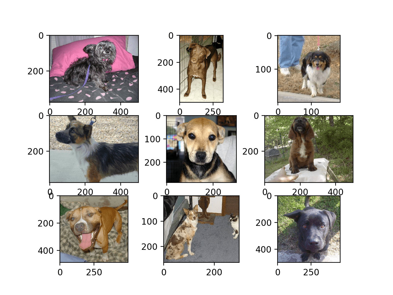
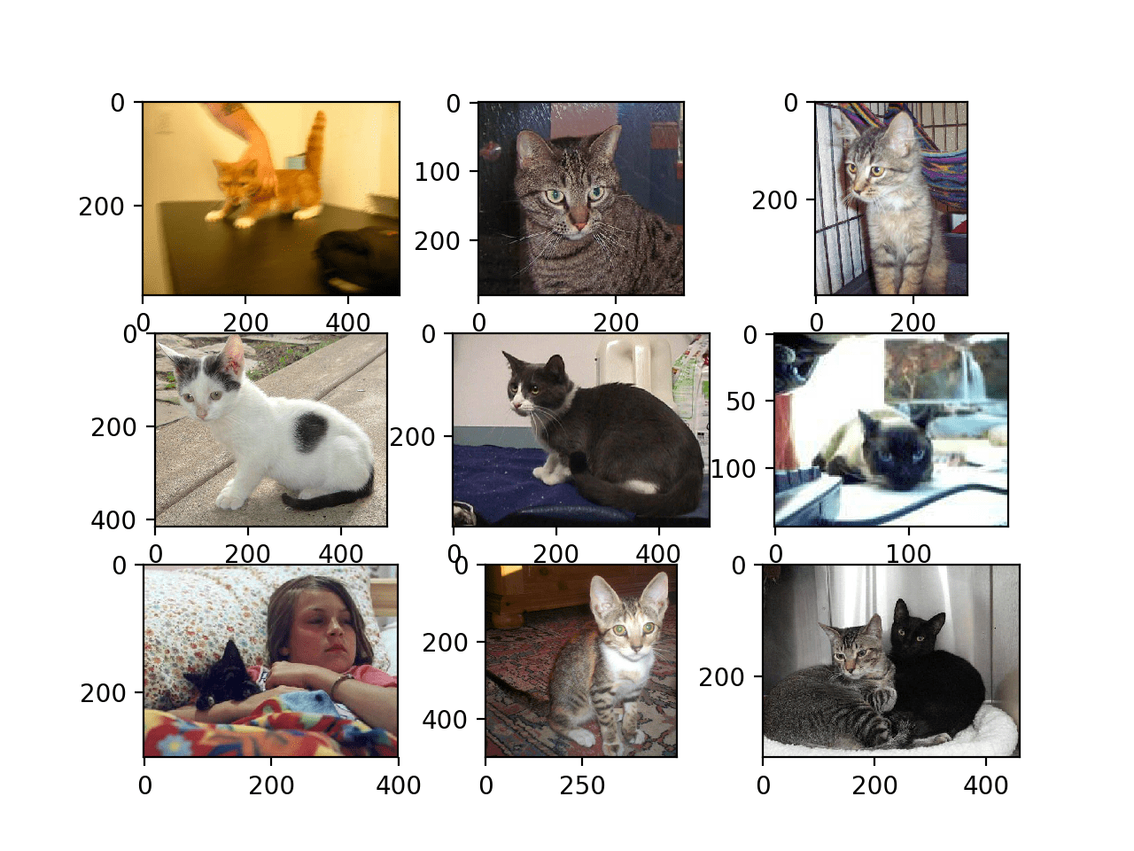
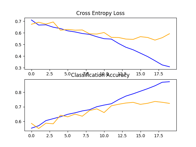
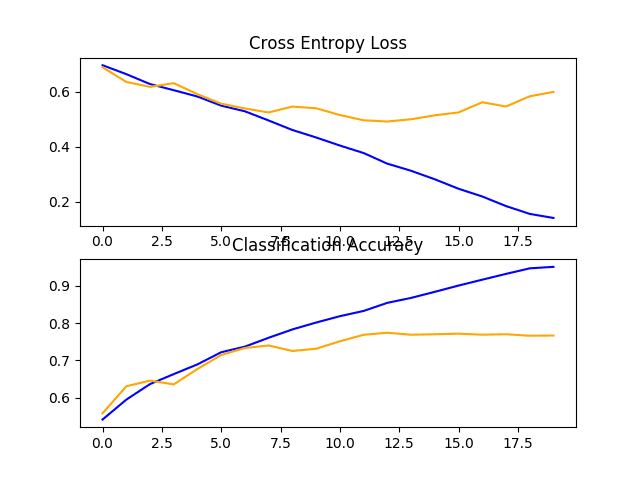
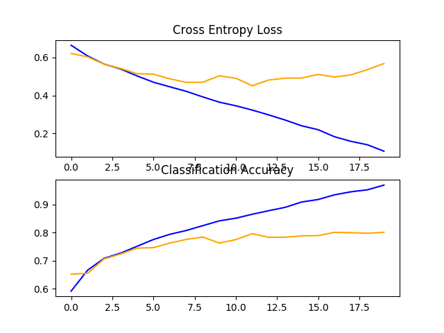
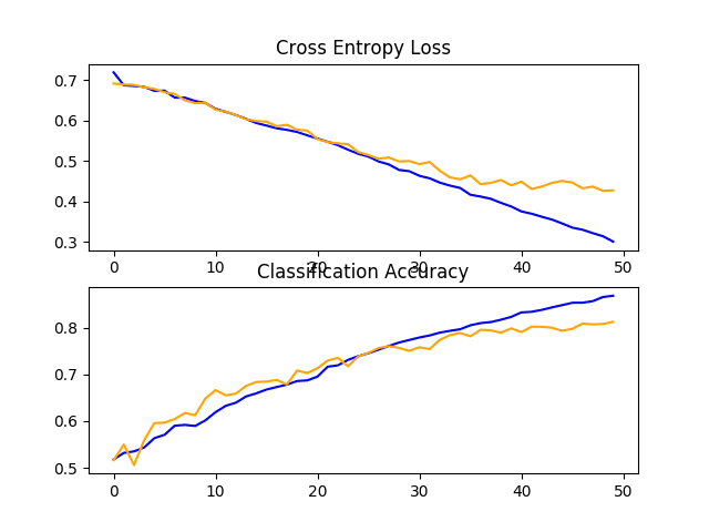
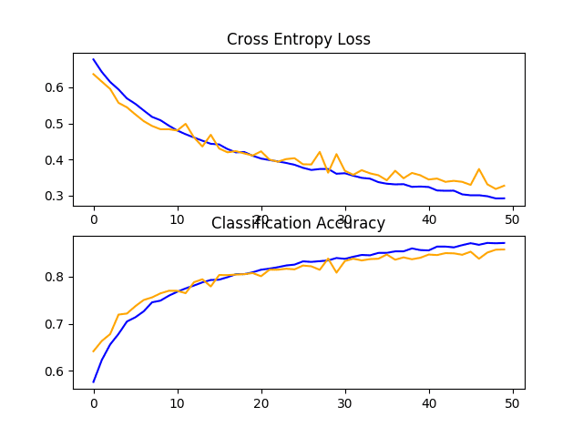
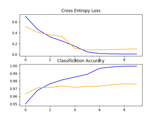
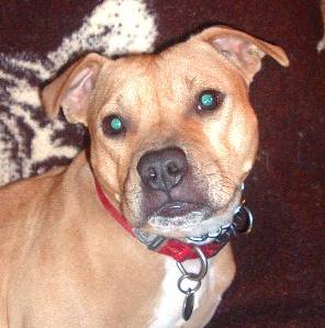


Thank you! This tutorial is amazing. I’ve gone through your example but was curious how long it took for your model to generate. The code has been running on a laptop for close to 4 hours now. Not sure if that is a long time or not. Thanks
I believe I ran it on AWS with a p3 instance (GPU). I don’t recall how long it took sorry. Perhaps a few hours?
Paul, I tried the model on Mac – ran without any issues, successfully compiled the code for all the test cases
Trained
500 cats, 500 dogs –
Test
250 cats + dogs
With large datasets, I ran out of memory – I will run it on cloud
Thank you! This tutorial is great. I’ve gone through your code with my own collected data set for fish species classification. It becomes a multi-class problem, but the model is not fit on that multi-class problem. I gain the accuracy of 66.667 for the final model you stated above. Any suggestion to increase the accuracy will be appreciated. Thanks
Well done!
Yes, I have some suggestions here:
https://machinelearningmastery.com/start-here/#better
you need to add a ‘softmax’ layer instead of sigmoid, right.
model.add(Dense(num_classes, activation=’softmax’)).
I hope it will work for you.
Hello. Tank you for this tutorial.
I am interested in something similar using R instead of Python. By chance do you know analogous code mainly for the data preparation.
Sorry, I don’t have examples of Keras in R.
Hello, thank you for this sharing, i started to learn your lessons from March 2019, really helpful ! Now I plan to go through your sample with my data set for children’s hand writing text classification, looking forward to your suggestions, thanks in advance!
The Chinese Text looks like “你”, “我”,”他”,”她” and etc, about 2000 in all, but they’re not print by computer but write by child and i have the picture of text.
Currently i have two ideas in my mind to do below job, they’re
Parent speak out the word and children do the listening homework, ( AI check the children if they write the correct texts.
1. The first one is train one super model to distinguish all the texts,
2. Train a model for each text and use this model to check children’s homework ( this could work because i do know what text the child is going to write )
which one do you think it’s better or do you have any other good suggests, thank you so much!
-Charles
Sounds like fun!
Perhaps try prototyping each and double down on the case that is the most interesting/fun/likely to pay off?
Hello Jason, when i try train one model, it seems fine but when i try to load the model it throws below error:
ValueError(‘Cannot create group in read only mode.’)
do you have any idea what’s wrong here?
thanks a lot!
i have fixed the failure, please ignore above question, i am now doing option 2 : pair compare, like the dog and cat, do you have any sample code for multiple compare? such as dog, cat, monkey, bird and etc.
Thanks!
No problem.
Yes, right here:
https://machinelearningmastery.com/how-to-develop-a-cnn-from-scratch-for-cifar-10-photo-classification/
I have not seen this error before, sorry.
Perhaps double check that all libraries are up to date?
Perhaps try searching/posting on stackoverflow?
Get it, i will try to lean 10 photo classification, i had fix the model load issue,
share the error in my case, maybe someone will meet the same issue, hope this helpful.
Charles : below code works fine with sample code but fail to load my text image trained model, wired to me
=============================================
from keras.models import load_model
loaded_model = load_model(‘text_model’)
Charles : i use another way to load, seems works fine for me :
=============================================
from keras.models import model_from_json
loaded_model = model_from_json(‘text_model’)
BTW, i have a question for dataset rotation, as i don’t have that many images, i tried to rotate the image in order to increase the dataset, i got classification accuracy quickly drop from 97% to 53%.
What i did is create 3 folders, copy my data set into each of them, then
folder 1. rotate image 90 degree
folder 2. rotate image 180 degree
folder 3. rotate image 270 degree
copy all images into folderX and train model base on all images.
More on model loading here:
https://machinelearningmastery.com/save-load-keras-deep-learning-models/
Perhaps try image augmentation instead:
https://machinelearningmastery.com/how-to-configure-image-data-augmentation-when-training-deep-learning-neural-networks/
Thanks for the totorial!
Do you have any example of image segmentation for feature selection before applying the classification model?
Actually, i am having problem with the region based image segmentation.
Here is my code!
# plot cat photos from the dogs vs cats dataset
from matplotlib import pyplot
from matplotlib.image import imread
from PIL import Image
from skimage.color import rgb2gray
import numpy as np
import cv2
import matplotlib.pyplot as plt
from scipy import ndimage
import os, sys
# define location of dataset
folder = ‘test/’
folder1 = ‘ (‘
folder2 = ‘)’
folder3 = ‘2/’
# plot first few images
path = ‘1/’
dirs = os.listdir( path )
def resize():
for item in dirs:
if os.path.isfile(path+item):
im = Image.open(path+item)
f, e = os.path.splitext(path+item)
g, d = os.path.splitext(folder3+item)
gray = rgb2gray(im)
gray_r = gray.reshape(gray.shape[0]*gray.shape[1])
for i in range(gray_r.shape[0]):
if gray_r[i] > gray_r.mean():
gray_r[i] = 3
elif gray_r[i] > 0.5:
gray_r[i] = 2
elif gray_r[i] > 0.25:
gray_r[i] = 1
else:
gray_r[i] = 0
gray = gray_r.reshape(gray.shape[0],gray.shape[1])
imResize = gray.resize((200,200), Image.ANTIALIAS)
imResize.save(g + ‘.jpg’, ‘JPEG’, quality=100)
resize()
i am getting the error ” if rgb.ndim == 2:
AttributeError: ‘JpegImageFile’ object has no attribute ‘ndim'”
Can you help!
Not exactly, but perhaps this model will help:
https://machinelearningmastery.com/how-to-train-an-object-detection-model-with-keras/
Hello Jason,
great tutorial as usual.
Could you maybe explain why you used SGD as GD optimizer?
Did you maybe try with RSMProp and Adam and empirically noticed a greater accuracy with SGD or is there a different reason?
Thanks
It is good to start with Adam or similar, but if you have time, SGD and fine tuning the learning rate and momentum can often give great or even better results.
can I compile and run the test harness for evaluating a model which contain only fully convolutional neural network blocks with out fully connected layers ( dense layers) for edge detection purposes thank you very much
Probably.
Hy I need your help. I am confused at that line of code.
history = model.fit_generator(train_it, steps_per_epoch=len(train_it),
validation_data=test_it, validation_steps=len(test_it), epochs=50, verbose=0)
I know here, train_it is the training images, which we are going to use for training purpose. But where you are passing the labels list of the data ? I know it is must to pass labels class as well for classification related problems.
Can you please help me out?
It fits the model.
We are using a data generator, you can learn more about it here:
https://machinelearningmastery.com/how-to-configure-image-data-augmentation-when-training-deep-learning-neural-networks/
Did I get it right that, when we use flow_from_directory method, then automatically the names of the folders (in which the training images are present) are used as the labels? is it true?
Yes, the folders in the directory represent the classes.
In your mentioned link, u did mention that
# create iterator
it = datagen.flow_from_directory(X, y, …)
mean you are passing X, and labels list as well. But in that classification problem, you are just passing the path of training images.. .
Please help me out. I am really confuse at that point. . .
The flow_from_directory() function takes a path, see here for an example:
https://machinelearningmastery.com/how-to-load-large-datasets-from-directories-for-deep-learning-with-keras/
Is that code open source? Can we use that code in our projects? Can anybody guide me in that regard . . .
My code is copyright, but you can use it in your own projects, more details here:
https://machinelearningmastery.com/faq/single-faq/can-i-use-your-code-in-my-own-project
I am not getting that why you did use two dense layers in the model. Moreover, what is the purpose of Dense layer and how you did choose the numbers of neuron in the dense layer. What is criteria of that selection. . .?
I used a little trial and error.
More here:
https://machinelearningmastery.com/faq/single-faq/how-many-layers-and-nodes-do-i-need-in-my-neural-network
As per my knowledge, we mention the number of total output classes in the dense layer, which is 2 in your case (Cats and Dogs), so why you mentioned 1 in dense layer ?
Second, what is the purpose of dense layer, which you added with 128 nodes at end?
Please help me to grab that concept?
The first dense layer interprets the features. The second makes a classification prediction.
Yes, I got it that second Dense layer make classification predication. But in your case there are two classes (Cats and Dogs) then why you are using 1 node on Dense layer..
model.add(Dense(1, activation=’sigmoid’))
So there should be 2, isn’t it?
The sigmoid activation function is used for binary classification problems.
A 0 is for the first class and a 1 is for the second class.
This is called a Bernoulli response.
Would this code work if I have a Cat and Dog in the same image. Is there a way for me to count the number of pets in the image.
No. The problem assumes one “thing” in the image that is a dog or a cat.
We have to make assumptions when framing a problem, e.g. to constrain the problem in order to make it easier to solve.
Hi there,
Thank you very much for this tutorial. It’s clearly explained and it’s working for me.
I want to extend the program and make it recognize in real-time using a camera. Is there’s any way that you can help? Or do you have a different tutorial for it?
You could use the model on each frame of video, or a subset of frames.
Hi Jason,
In the transfer learning section, i do not see how you initialize the weights on VGG16 to “imagenet”. So are you just using the VGG16 structure or using it with the weights initialized. I could be missing something here
Thanks,
They are initialized to imagnet by default in Keras.
Thank you for this tutorial. Your tutorial is amazing and I found it very useful. I do not understand why did we pass only training data to save the final model? do not we need to pass validation data as well? Why did you use fit_generator instead of fit? When I run the saved model, during training I did not get any feedback or output while running the transfer learning I get output on each step and I can see the loss is going done. How can I change the save model section to get feedback from the model while it is training?
We used fit_generator() because we used progressive loading.
You can change verbose=1 or verbose=2 to get feedback during training.
Thank you.
I am trying to add the class activation map to your final model code. Based on my understanding all I need to do the following:
replace
# add new classifier layers
flat1 = Flatten()(model.layers[-1].output)
class1 = Dense(128, activation=’relu’, kernel_initializer=’he_uniform’)(flat1)
output = Dense(1, activation=’sigmoid’)(class1)
with
# add new classifier layers
class1 = GlobalAveragePooling2D()(model.layers[-1].output)
output = Dense(1, activation=’sigmoid’)(class1)
Then train the model and finally, generate the heat map. I am not sure my heatmap is correct. Do you have any tutorial that I can follow step by step to generate the Class activation map?
Thanks
Great question.
I don’t have an example, but thanks for the suggestion!
Great tutorial!
A question, in the 3% that model.predict(img) does not recognize a dog or a cat, what does he return?
Thanks.
It makes an error. Dog when it is a cat or cat when it is a dog.
In fact, if you look at the hard cases, it get them wrong because they are hard or the data is rubbish.
HI again, I tried to modify your code to use model.fit() instead of model.fit_generator() but I get a very bad result, actually, my loss gets close to zero on 1st epoch.
I tried everything to the best of my knowledge to improve the result but I failed. I appreciate if you look at my code and tell me what is wrong with this code?
This is the output while I was training my model:
++++++++++++++++++++++++++++++++++++++
Epoch 1/10
32/18750 […………………………] – ETA: 46:03 – loss: 3.0541 – acc: 0.2812
64/18750 […………………………] – ETA: 23:30 – loss: 1.5280 – acc: 0.6406
96/18750 […………………………] – ETA: 15:58 – loss: 1.0187 – acc: 0.7604
128/18750 […………………………] – ETA: 12:11 – loss: 0.7641 – acc: 0.8203
160/18750 […………………………] – ETA: 9:55 – loss: 0.6113 – acc: 0.8562
192/18750 […………………………] – ETA: 8:24 – loss: 0.5094 – acc: 0.8802
224/18750 […………………………] – ETA: 7:20 – loss: 0.4366 – acc: 0.8973
256/18750 […………………………] – ETA: 6:31 – loss: 0.3820 – acc: 0.9102
288/18750 […………………………] – ETA: 5:53 – loss: 0.3396 – acc: 0.9201
320/18750 […………………………] – ETA: 5:23 – loss: 0.3056 – acc: 0.9281
352/18750 […………………………] – ETA: 4:58 – loss: 0.2778 – acc: 0.9347
384/18750 […………………………] – ETA: 4:38 – loss: 0.2547 – acc: 0.9401
416/18750 […………………………] – ETA: 4:21 – loss: 0.2351 – acc: 0.9447
448/18750 […………………………] – ETA: 4:06 – loss: 0.2183 – acc: 0.9487
480/18750 […………………………] – ETA: 3:53 – loss: 0.2038 – acc: 0.9521
512/18750 […………………………] – ETA: 3:42 – loss: 0.1910 – acc: 0.9551
544/18750 […………………………] – ETA: 3:32 – loss: 0.1798 – acc: 0.9577
576/18750 […………………………] – ETA: 3:23 – loss: 0.1698 – acc: 0.9601
608/18750 […………………………] – ETA: 3:15 – loss: 0.1609 – acc: 0.9622
640/18750 [>………………………..] – ETA: 3:07 – loss: 0.1528 – acc: 0.9641
672/18750 [>………………………..] – ETA: 3:01 – loss: 0.1455 – acc: 0.9658
704/18750 [>………………………..] – ETA: 2:55 – loss: 0.1389 – acc: 0.9673
736/18750 [>………………………..] – ETA: 2:50 – loss: 0.1329 – acc: 0.9688
768/18750 [>………………………..] – ETA: 2:47 – loss: 0.1273 – acc: 0.9701
800/18750 [>………………………..] – ETA: 2:47 – loss: 0.1223 – acc: 0.9712
18750/18750 [==============================] – 84s 4ms/step – loss: 0.0052 – acc: 0.9988 – val_loss: 1.2813e-07 – val_acc: 1.0000
Here is my code:
+++++++++++++
import keras
from keras.layers import Dropout
from keras.models import Sequential
from keras.layers import Conv2D
from keras.layers import MaxPooling2D
from keras.layers import Dense
from keras.layers import Flatten
from keras.optimizers import SGD
from sklearn.model_selection import train_test_split
from sklearn.metrics import classification_report
from keras.callbacks import TensorBoard, ModelCheckpoint, EarlyStopping
import numpy as np
import os
import cv2
import random
import matplotlib.pyplot as plt
from os import listdir
from numpy import save, load
import time
data_dir = os.path.join(“data”,”finalize_dogs_vs_cats”)
image_size = 224
EPOCHS = 10
num_classes = 2
save_model = ‘Models\simple_nn.model’
save_label = ‘Models\simple_nn_lb.pickle’
save_plot = ‘Models\simple_nn_plot.png’
data_path = ‘data/dogs-vs-cats’
photoes_name = os.path.join(data_path, ‘simple_dogs_vs_cats_photos.npy’)
labels_name = os.path.join(data_path, ‘simple_dogs_vs_cats_labels.npy’)
def prepare_data(in_data_dir, in_image_size):
imagePaths = []
# define location of dataset
folder = os.path.join(data_path, ‘train/’)
# enumerate files in the directory
for file in listdir(folder):
imagePath = os.path.join(folder, file) # create path to dogs and cats
imagePaths.append(imagePath)
random.seed(42)
random.shuffle(imagePaths)
data, labels = list(), list()
for imagePath in imagePaths:
image = cv2.imread(imagePath)
image = cv2.resize(image, (in_image_size, in_image_size))
data.append(image)
label = imagePath.split(os.path.sep)[-2]
# determine class
output = 0.0
if label.lower().startswith(‘cat’):
output = 1.0
labels.append(output)
# scale the raw pixel intensities to the range [0, 1]
data = np.array(data, dtype=”float”) / 255.0
labels = np.array(labels)
print(data.shape, labels.shape)
# save the reshaped photos
save(photoes_name, data)
save(labels_name, labels)
return data, labels
def define_model():
model = Sequential()
model.add(Conv2D(32, (3, 3), activation=’relu’, kernel_initializer=’he_uniform’, padding=’same’, input_shape=(image_size, image_size, 3)))
model.add(MaxPooling2D((2, 2)))
model.add(Dropout(0.2))
model.add(Conv2D(64, (3, 3), activation=’relu’, kernel_initializer=’he_uniform’, padding=’same’))
model.add(MaxPooling2D((2, 2)))
model.add(Dropout(0.2))
model.add(Conv2D(128, (3, 3), activation=’relu’, kernel_initializer=’he_uniform’, padding=’same’))
model.add(MaxPooling2D((2, 2)))
model.add(Dropout(0.2))
model.add(Flatten())
model.add(Dense(128, activation=’relu’, kernel_initializer=’he_uniform’))
model.add(Dropout(0.5))
model.add(Dense(num_classes, activation=”softmax”))
# compile model
opt = SGD(lr=0.0001, momentum=0.9)
model.compile(optimizer=opt, loss=’categorical_crossentropy’, metrics=[‘accuracy’])
model .summary()
return model
def main():
do_data_preparation = False
if(do_data_preparation):
data, labels = prepare_data(data_dir, image_size)
data = load(photoes_name)
labels = load(labels_name)
(trainX, testX, trainY, testY) = train_test_split(data, labels, test_size=0.25, random_state=42)
trainY = keras.utils.to_categorical(trainY, num_classes)
testY = keras.utils.to_categorical(testY, num_classes)
model = define_model()
NAME = f’Cat-vs-dog-cnn-64×2-{int(time.time())}’
filepath = “Model-{epoch:02d}-{val_acc:.3f}” # unique file name that will include the epoch and the validation acc for that epoch
checkpoint = ModelCheckpoint(“Models/{}.model”.format(filepath, monitor=’val_acc’, verbose=1, save_best_only=True,
mode=’max’)) # saves only the best ones
tensorBoard = TensorBoard(log_dir=’Models\logs\{}’.format(NAME))
early_stop = EarlyStopping(monitor=’val_loss’, patience=1, verbose=1, mode=’auto’)
callback_list = [checkpoint, early_stop, tensorBoard]
# train the neural network
H = model.fit(trainX, trainY, validation_data=(testX, testY),
epochs=EPOCHS, batch_size=32, verbose=1, callbacks=callback_list)
# evaluate the network
print(“[INFO] evaluating network…”)
predictions = model.predict(testX, batch_size=32)
print(classification_report(testY.argmax(axis=1),
predictions.argmax(axis=1), target_names=num_classes))
# plot the training loss and accuracy
N = np.arange(0, EPOCHS)
plt.style.use(“ggplot”)
plt.figure()
plt.plot(N, H.history[“loss”], label=”train_loss”)
plt.plot(N, H.history[“val_loss”], label=”val_loss”)
plt.plot(N, H.history[“acc”], label=”train_acc”)
plt.plot(N, H.history[“val_acc”], label=”val_acc”)
plt.title(“Training Loss and Accuracy (Simple NN)”)
plt.xlabel(“Epoch #”)
plt.ylabel(“Loss/Accuracy”)
plt.legend()
plt.savefig(save_plot)
# save the model and label binarizer to disk
print(“[INFO] serializing network and label binarizer…”)
model.save(save_model)
main()
I’m eager to answer specific questions, but I don’t have the capacity to review and debug your code, sorry.
I have some suggestions here:
https://machinelearningmastery.com/faq/single-faq/can-you-read-review-or-debug-my-code
I’m bit of a noob here but can you explain how a low loss and high accuracy is a bad result ? How are you inferring it just on the basis of that? The validation accuracy looks good too! So how is it a bad result? Idk if I’m missing something here
how do we decide if the model.predict(img) gives the output as 1 and then on what basis this 1 means Dog ?
Great question.
We prepare the data by mapping classes to integers. It just so happens that we mapped cat to 0 and dog to 1, but we could map it any way we wish.
Hi Jason,
You are amazing zing !!. You replied me within few hours.It’s great.
BTW, I missed below lines. That’s why I had to ask that question.
Note: the subdirectories of images, one for each class, are loaded by the flow_from_directory() function in alphabetical order and assigned an integer for each class. The subdirectory “cat” comes before “dog“, therefore the class labels are assigned the integers: cat=0, dog=1. This can be changed via the “classes” argument in calling flow_from_directory() when training the model.
Thanks for sharing your knowledge to the world.
Thanks.
No problem, I’m happy the tutorial helped!
Hi,
I have also a binary classification problem. I want to classify synthetic depth images against real depth images. I developed a binary classifier like your model but the accuracy remains at 0.5 after 50 epochs and the loss gets 0.7. I have 500images from each class -> totally 1000 images. Images are grayscale.
Do you have any idea, how I Could improve the problem?
Here you can find an example image pair: https://github.com/junyanz/pytorch-CycleGAN-and-pix2pix/issues/735
Best Regards
Yes, you can learn how to diagnose issues with models and improve performance here:
https://machinelearningmastery.com/start-here/#better
I just want to thank you for the time and efforts.
Whenever I try to give the model a picture that does NOT include a cat or dog, it predicts a dog or cat.
How to show the percentage of assumption accuracy?
and how to print a message that the model is not sure or “No cats nor dogs are found”
if result[0] == 0:
print(‘I think this is a Dog’)
elif result[0] == 1:
print(‘I think this is a Cat’)
else:
print(‘No cats nor dogs are found’)
Yes, the model is only trained on dogs/cats therefore that is all it expects to see during inference.
You can call predict() with one image to get a probability of the prediction.
There is no “unknown” class, you could train it that way if you wanted.
Thank you so much Jason for writing all these articles and tutorials about ML, and I appreciate all the effort you do to answer every single question on the blog.
I think you are a superhero.
<3
Thanks for your support, I deeply appreciate it!
I have a similar situation, would like prediction to be like “dog”, or “cat”, or “neither”. How best to train for an “unknown” class please? Would I just use random photos without cats or dogs for the unknown class?
You need photos in your training dataset that don’t match either class (and are like what you expect to see in the future) and train the model to assign the class “neither” to these photos.
I am unable to understand that . . .
steps_per_epoch=len(train_it)
I mean why you did mention that steps_per_epoch = len(train_it) in the code?
It indicates that the number of “steps” in one epoch is the number of samples (images) in the training dataset.
For more on samples and epochs, see this:
https://machinelearningmastery.com/faq/single-faq/what-is-the-difference-between-a-batch-and-an-epoch
Hy I need your help.
I am trying to run just one block of CNN model on limited data for testing purpose. But with same parameters I get different accuracy output, every time I run the code.
How I can get the same results on every time I run the code?
I tried to do it by fixing the seeds using numpy.random.seeds. . .But it is not working.
Can you help me out to fix it?
This is a very common question that I answer here:
https://machinelearningmastery.com/faq/single-faq/why-do-i-get-different-results-each-time-i-run-the-code
Hy Jason,
Actually, I am training my model on limited data with limited numbers of epochs. I have also fixed the seeds (as i mentioned in my question). But still I am facing different output on same configuration, every time I run the model. . . .
Can you please suggest me that what else can be the possible issue ?
Yes, fixing the seed might be a loosing battle, I don’t recommend it:
https://machinelearningmastery.com/reproducible-results-neural-networks-keras/
C:\Users\Yali\Desktop\dogvscat\data\train\
Traceback (most recent call last):
File “data_processing.py”, line 25, in
photo = load_img(image_path + file, target_size=(200, 200))
File “C:\Users\Yali\Anaconda3\envs\DC\lib\site-packages\keras_preprocessing\image\utils.py”, line 110, in load_img
img = pil_image.open(path)
File “C:\Users\Yali\Anaconda3\envs\DC\lib\site-packages\PIL\Image.py”, line 2770, in open
fp = builtins.open(filename, “rb”)
PermissionError: [Errno 13] Permission denied: ‘C:\\Users\\Yali\\Desktop\\Melanoma\\data\\train\\cat’
Hi, I met this problem, could you help me?
Looks like a problem with your Python installation?
Perhaps try re-installing:
https://machinelearningmastery.com/setup-python-environment-machine-learning-deep-learning-anaconda/
HI, I had the problem as well and have it with:
solved
pip pytest-shutil install
sorry, my problem did not solve itself.
I still get the error:
copyfile (src, dst)
File “C: \ Python \ Python37 \ lib \ shutil.py”, line 120, in copyfile
with open (src, ‘rb’) as fsrc:
PermissionError: [Errno 13] Permission denied: ‘train // cats’
maybe the problem is with the use of backslash while it should use slash instead?
I had an error that i dont know how can fix it. I got the error during model creation. I shared in below.
TypeError: fit_generator() got an unexpected keyword argument ‘step_per_epoch’
Sorry to hear that I have some suggestions here:
https://machinelearningmastery.com/faq/single-faq/why-does-the-code-in-the-tutorial-not-work-for-me
hi jason wonderful article.
I have question that most of the image classification problems i have seen are trying to classify ,all the categories that are given to them.
what is meant to say is that suppose we want to classify 10 birds and 10 animals so total 20 categories then how can we make a CNN which first decide whether the image is bird or animal and then based on that it classify on the basis of that in which of the 10 categories it falls.
would ‘t it be easy for CNN to classify in this way rather than classifying whole 20 categories ?
is there any such implementation of CNN?
Good question, that might be a two-step classification problem, e.g. first classify type of animal, then specific species.
It is often more effective to predict the species directly. The reason is that errors on the first step make the second step irrelevant.
Nevertheless, you can try both approaches for your dataset and compare the results.
Can you share the final trained model – I’m curious how this compares to several other solutions
Sorry, I don’t share final models because of their large size.
Thanks.One of the best article for Image classification I ever come across.But I am little confused about steps_per_epoch.you have defined it as len(train_it) but I have seen it defined as len(train_it)/batch_size in few other blogs .
I am getting a different dataset with total 8000 images of cat and dog and getting 70% accuracy(You are getting 85%.Wow) .I am using 3 layer VGG with dropout and augmentation.
Can I extend this VGG 3 model for multi class(around 10 classes) ?
Thanks.
train_it is already split into batches.
Yes, VGG is a multi-class model under the covers.
Hy, I need your help.
I’ve used ImageDataGenerator and flow_from_directory for training and validation.
By using model checkpoints, I have got my trained model name as model.hdf5.
Now I want to make prediction on a single image. How I can do that? In the training data my input_shape is (90,90,3)
Can you please help me out that how I can make prediction on a single image?
See the section “How to Finalize the Model and Make Predictions”
I show exactly this!
I have another question.
Why you did do that in making prediction on single image.
img = img – [123.68, 116.779, 103.939]
What are these values, which you just subtracted?
When I applied your code for prediction on single image, I got these results.
[0. 1. 0. 0.]
What does that mean? What these results are showing.
Please answer in detail
As I mention in the post – to prepare the image in the same way as the training data was prepared:
It is a nice post,But sir I have a problem in which my dataset is in following form
I want to maintain the data set like above mention,So I used Data Image Generator to the problem like this.Can You guide me about this
Perhaps collapse the style directories into class directories.
You could write a script to copy the files for you or you could do it manually. Alternately, you could write a custom data generator to load the data with this structure. I have examples on the blog you could use as a starting point.
Also see this:
https://machinelearningmastery.com/how-to-load-large-datasets-from-directories-for-deep-learning-with-keras/
style is a sub diretory………which contain images
Hi Jason,
I used the following 2D CNN for binary classification with the dataset {14189 samples (rows, 400 features (columns),1 label (column)}. The data shape is (20,20,1) as input in the first zero-padding layer. Now I want to add the LSTM layer after the last 2D CNN block in my code. Please let me know about the LSTM layer code. My 2D CNN code and data shape are given below:
trn_file = ‘PSSM_4_Seg_400_DCT_1_14189_CNN.csv’
nb_classes = 2
nb_kernels = 3
nb_pools = 2
# load training dataset
dataset = numpy.loadtxt(trn_file, delimiter = “,”) # , ndmin = 2)
print(dataset.shape)
# split into input (X) and output (Y) variables
X = dataset[:,1:401].reshape(len(dataset),20,20,1)
Y = dataset[:, 0]
model = Sequential()
model.add(ZeroPadding2D((1, 1), input_shape = ( 20, 20,1)))
model.add(Conv2D(4, nb_kernels, nb_kernels, activation = ‘relu’))
model.add(MaxPooling2D(strides = (nb_pools, nb_pools), dim_ordering = ‘th’))
model.add(ZeroPadding2D((1, 1)))
model.add(Conv2D(8, nb_kernels, nb_kernels, activation = ‘relu’))
model.add(MaxPooling2D(strides = (nb_pools, nb_pools), dim_ordering = ‘th’))
model.add(ZeroPadding2D((1, 1)))
model.add(Conv2D(16, nb_kernels, nb_kernels, activation = ‘relu’))
model.add(MaxPooling2D(strides = (nb_pools, nb_pools), dim_ordering = ‘th’))
## add the model on top of the convolutional base
model.add(Flatten())
model.add(Dense(32, activation = ‘relu’))
model.add(Dropout(0.5))
model.add(Dense(nb_classes)) #fully connected layer
model.add(Activation(‘sigmoid’))
LSTM would not be appropriate for classifying images.
yeah, LSTM would not be appropriate for image classification. I just want to show the performance of LSTM for images. Please let me know LSTM code after last CNN layer.
It’s not just “inappropriate”, I don’t believe it is feasible.
Hi Jason,
When we preprocess the data without using ImageDataGenerator, as in the optional example you provide for resizing the images that takes 12 gigabytes of RAM to run, why are the pixel values not rescaled to 1.0/255.0 as is done with the ImageDataGenerator?
Your articles are awesome!!!
Thanks.
Sorry I don’t understand the question as the ImageDataGenerator is used in all examples.
If you mean, why do we sometimes normalize and sometimes standardize the pixels – then the former is a good practice, the latter is a requirement for using the pre-trained models.
The example is provided in the part of this article titled “Pre-Process Photo Sizes (Optional)”, where you write
“If we want to load all of the images into memory, we can estimate that it would require about 12 gigabytes of RAM.”
In that example the images are never rescaled.
The image is resized as part of a call to load_img(), e.g. to the size of 200 pixels width and height.
Oh Yikes! I meant rescaling the pixels, not resizing, sorry.
This is done in the examples with ImageDataGenerator you provide as follows:
datagen = ImageDataGenerator(rescale=1.0/255.0)
My question is:
At what point during the example “Pre-Process Photo Sizes (Optional)” is this rescaling of the pixel values done?
Sorry about the misleading question
It’s not. Pixel scaling is done when we fit the model.
Hy,
I want to ask that during the training the model we have to define various layers like conv, activation, pooling, dense etc. From these layers the training data has to pass various stages.
Then why we do not have to define these various layers during the testing? I meant to say that we should also mold our data using various layers, as we do during the training stages. In short, we should also apply the various layers on testing data, then make predictions using trained model. . .
Waiting for your reply. . .
During testing, the model has already been defined and trained. We simply load it and use it like a “program”.
Hi,
I’ve implemented this algorithm (code example) using labeled satellite photos (binary prediction – has a certain object or not) instead of cats and dogs.
My training and test accuracy is pretty good around 95% and 82% respectively.
However, when I run the model on a large holdout set (14K images), I essentially get a large number of false positive predictions with much lower accuracy
and virtually no true positives.
I will say I only have a training set of about 1400 images and test set of 1120 images, so I admit my data is small.
However, I’m not sure why i’m seeing such poor performance on holdout ? My assumption is the model is overfitting ?
Well done!
Perhaps the hold out set is significantly different from the train set?
Perhaps the model overfit the training set?
This can help in diagnosing the problem:
https://machinelearningmastery.com/start-here/#better
Hello, Im getting below error when i run the code.
AttributeError: module ‘tensorflow’ has no attribute ‘get_default_graph’
Thanks,
Karthik
Sorry to hear that, I have some suggestions here:
https://machinelearningmastery.com/faq/single-faq/why-does-the-code-in-the-tutorial-not-work-for-me
i have a train model In cnn now i want to test a random image how can i do this….?
Load the image and use the model to make a prediction.
See the section “Make Prediction” for an exact example of this.
Very good article. It was very well written and reasonably understandable for a ML mere mortal such as myself. After training the model with the set of 25k images, it very reliably predicted cat/dog when I fed it random pictures of said animals. For fun, I fed it a picture of a boat, and it told me it was neither a cat nor a dog. Success! However, when I fed it a picture of a mouse, the prediction thought it was a cat, and when fed a picture of a kangaroo, it said it was a dog. Is there a way to make this more accurate? Perhaps using a much larger data set?
Thanks.
Very cool!
Yes, you could feed in images of other stuff and encourage it to predict a third label of “I don’t know” or “not cat or dog”.
Thanks for the reply Jason. Would a much larger data set be the way to lessen the kangaroo/mouse false positives? Or should I look elsewhere?
It may, but it is good to test many candidate solutions to see what gives the biggest effect.
How did it give you a boat ?
Doesn’t predict always return either 0 or 1 ?
1 other question I had was on the target size argument. My images are originally 640×640 satellite images.
However, if I want to use a pretrained model like MobileNet, it appears the max size I can use is 224.
I’m ok with that so long as it does not reduce performance or accuracy. I’m not clear what the impact is of reducing target_size from 640 to 224 ?
I believe most models, like the vgg will scale up with image size.
I recommend running tests to calculate the impact of image scaling, if it is a concern.
Hi Jason, I have a question about ImageDataGenerator.flow_from_directory, i am using VGG-16 for transfer learning, how to add VGG16 preprocess_input for datagen.flow_from_directory and model.fit_generator? the code is as below:
datagen = ImageDataGenerator()
train_gen = datagen.flow_from_directory()
model.fit_generator(train_gen)
where to add the preprocess_input ?
You can use the example here:
https://machinelearningmastery.com/how-to-load-large-datasets-from-directories-for-deep-learning-with-keras/
Hi, great blog!
could one also distinguish whether a cat has booty in its mouth or not?
I have pictures of my cat with prey and picture of the cat without prey.
Or would the comparison only prove that it is a cat?
Yes, but you would have to train the model on that class, e.g. “cat” vs dog vs “cat with something in month”
Thanks for the answer 🙂
Would it be enough, a label :
my cat with booty
and a label:
my cat without booty?
Yes, if that is the goal of the project.
Hi.. do you have a example to use the cnn to comparison pets and not only recognize? Like, I have a picture of my dog and I want to know if my dog is in other pictures of my dataset.
I don’t if I was clearly. But is like to know if a specific pet is in other pictures.
Could you help me?
Sounds like image search. Sorry, I don’t.
Hi, I have another question:
When running the script
“vgg16 model used for transfer learning on the cats and cats dataset”
my computer always crashes. Unfortunately, I have only 8 RAM work spreader.
Can I change something in the settings for it to go through?
Perhaps try using progressive loading:
https://machinelearningmastery.com/how-to-load-large-datasets-from-directories-for-deep-learning-with-keras/
Perhaps try running it on an ec2 instance:
https://machinelearningmastery.com/develop-evaluate-large-deep-learning-models-keras-amazon-web-services/
hi, maybe I was wrong.
I only used my pictures, max 150, per label for the realization
All other scripts worked, except for the script:
“vgg16 model used for transfer learning on the cats and cats dataset”
Here are the images for creating the VGG16 model converted. (if I understood that correctly)
The script also starts, but after a short time the process freezes and eventually comes from Windows the message that a problem has occurred and the computer must be restarted. This may actually only have to do with the memory.
Perhaps the model itself is too large for your machine?
Perhaps try running on aws ec2?
Do you have an example, how to upload the local images into the AWS and then train with the python scripts?
In your blog:
https://machinelearningmastery.com/develop-evaluate-large-deep-learning-models-keras-amazon-web-services/
is it all about the establishment of the AWS. But how does it continue?
I want to run all the scripts from the example of you in the AWS and then save the created model locally, so I can use in my program.
Yes, I show how to copy files to an AWS instance here:
https://machinelearningmastery.com/command-line-recipes-deep-learning-amazon-web-services/
I have a question on this statement regarding improvements to the pretrained VGG16 model:
“There are many improvements that could be made to this approach, including adding dropout regularization to the classifier part of the model and perhaps even fine-tuning the weights of some or all of the layers in the feature detector part of the model.”
How would I add dropout reg. to the layers already contained in the VGG16 model ?
How would I fine-tune the weights of some or all of the layers ?
You can re-define the abstract model to have dropout layers whilst using the same weight layers. Some work would be required, sorry, I don’t have an example.
Fine tuning means training on your dataset with a small learning rate.
Hi,
I tried … but:
I’m a bit desperate.
I could not choose the AWS from your example, since I can only opt for free products.
Then I set up an AWS following the instructions below.
https://aws.amazon.com/de/getting-started/tutorials/launch-a-virtual-machine/
I thought I could install an environment with Keras and Tensorflwo here.
Access via Git-Bash works.
tensorflow_p36
it does not work 🙁
‘source activate tensorflow_p36’
Do you have an idea?
I found your tutorial to be very helpful for dogs Vs Cats classification. However do you have any tutorial that walks us through how to submit our model prediction on kaggle? I am very new to programming and have never participated in any kaggle competitions so would be very helpful if I can follow any of your tutorials for that
Thanks.
No, sorry, I don’t have a tutorial on that topic.
Hi, I am trying to run the load_image and run_example functions using the plain vanilla model (NON Transferring learning , not VGG 16), but all predictions are zero. Do I need to make a small adjustment to the functions load_image and run_example (i.e., rescale ?) so the plain vanilla model can work properly ?
Perhaps, and the model may require careful choice of learning rate.
I don’t think it’s the learning rate as the train and validation results are near 90%. What’s happening is when I attempt to predict on a holdout set of images using the saved model via run_example, I get 100% zero predictions. I believe i need to adjust the code in load_image and run_example functions to work for your first CNN model which does not use transfer learning ?
Perhaps confirm that you are preparing the test data in an identical manner to the training data, e.g. pixel scaling.
Hi,
I have now come so far that I can run the code on a jupyter notebook.
Unfortunately, I get an error message:
KeyError traceback (most recent call last)
in ()
68
69 # entry point, run the test harness
—> 70 run_test_harness ()
in run_test_harness ()
65 print (‘>% .3f’% (acc * 100.0))
66 # learning curves
—> 67 summarize_diagnostics (history)
68
69 # entry point, run the test harness
in summarize_diagnostics (history)
38 pyplot.subplot (212)
39 pyplot.title (‘Classification Accuracy’)
—> 40 pyplot.plot (history.history [‘accuracy’], color = ‘blue’, label = ‘train’)
41 pyplot.plot (history.history [‘val_accuracy’], color = ‘orange’, label = ‘test’)
42 # save plot to file
KeyError: ‘accuracy’
3 functions do not seem to work.
I use a jupyter notebook with the “conda_tensorflow_p36”
I recommend not running in a notebook, and instead run from the command line:
https://machinelearningmastery.com/faq/single-faq/how-do-i-run-a-script-from-the-command-line
Hi Jason, this is really a helpful tutorial on the topic.
I have been reading from different sources, and have a couple of questions though.
1. For a classification problem, should the labels be categorical encoded or one-hot encoded, for example, using the to_categorical command?
For binary classification, there are only 2 classes, 0 and 1.
But how to label when there are >2 classes?
2. In the output layer, you use Dense(1) with sigmoid activation.
I have seen the use of Dense(2) with softmax activation, on another website, for binary classification.
What guides this choice? Are both options equivalent?
Thanks in advance for your response 🙂
Yes, one hot encoding is used for class labels, see this:
https://machinelearningmastery.com/why-one-hot-encode-data-in-machine-learning/
Yes, for multi-class the output is changed to n node for the n classes and the softmax activation.
I have tens of examples, perhaps start here:
https://machinelearningmastery.com/multi-class-classification-tutorial-keras-deep-learning-library/
Hi Jason, Thanks for the quick reply.
Another question: what metric should be used if there is imbalance in the number of images in the different classes, say 9:1 in the 2 classes?
Usually most deep learning tutorials show loss and accuracy. But accuracy is not supposed to be a good metric in case of data imbalance
You’re welcome.
Great question.
If both classes are equal, g-mean, if not, f-measure. If you are predicting probabilities roc auc or pr auc.
Does that help?
Sorry, it is not very clear to me. Did you mean F1 Score?
And what metric should be used for multi-class classification with data imbalance?
F1-score is the F-measure.
You can use the same measures.
Hi Jason, My understanding is that the default metric in keras is accuracy.
How do we obtain F1 score on the test dataset?
Another question, what will be the value of class_mode in the iterator for a multi-class problem?
No, the default is the loss you have chosen to optimize.
Here are examples of using other metrics:
https://machinelearningmastery.com/how-to-calculate-precision-recall-f1-and-more-for-deep-learning-models/
class_mode would be set to ‘categorical’. You can see the API here:
https://keras.io/preprocessing/image/
Hi Jason,
I have data imbalance among the classes, and I am getting low accuracy on both train and test set.
I am trying out data augmentation and model improvement (changing the number of layers and nodes).
I would also like to “see the predictions” for some examples in the test data, and what their actual class label was. Any idea/ code how to do this, since I am using generator functions (model.fit_generator and model.evaluate_generator) to fit and evaluate the model performance?
I have checked your tutorial
https://machinelearningmastery.com/how-to-calculate-precision-recall-f1-and-more-for-deep-learning-models/
https://machinelearningmastery.com/custom-metrics-deep-learning-keras-python/
Although I can readily compute the metrics for numeric data, I am unsure how to do this for custom images.
Thanks in advance.
The metrics operate on the predictions, not the images.
Hi Jason,
Thanks for the reply.
I am using this tutorial to develop a sample classifier for 3 classes – all images are in grayscale.
I have modified the first line in the model definition to:
model.add(Conv2D(32, (3, 3), activation=’relu’, kernel_initializer=’he_uniform’, padding=’same’, input_shape=(200, 200, 1)))
However, when I run model.fit_generator, I get the following error:
ValueError: Error when checking input: expected conv2d_1_input to have shape (200, 200, 1) but got array with shape (200, 200, 3)
But I have run a check on all the images with the command
image_name.mode (Pillow library)
All images returned ‘L’, which would indicate grayscale.
Any suggestions?
The error suggests your images have 3 channels. Perhaps change them to grayscale.
This might help:
https://machinelearningmastery.com/how-to-load-and-manipulate-images-for-deep-learning-in-python-with-pil-pillow/
Hi,
Adding the color_mode option solved the issue.
train_it = train_datagen.flow_from_directory(‘./runData/train/’, color_mode=’grayscale’, class_mode=’categorical’, batch_size=64, target_size=(200, 200))
test_it = test_datagen.flow_from_directory(‘./runData/test/’, color_mode=’grayscale’, class_mode=’categorical’, batch_size=64, target_size=(200, 200))
==========================================================
Another question: what does ’32/32′ mean? I obtain it during model fitting.
Epoch 1/50
32/32 [==============================] – 199s 6s/step – loss: 10.2217 – acc: 0.3450 – val_loss: 11.4814 – val_acc: 0.2877
Happy to hear that!
Hello Jason,
I have a basic question about the deep learning model – my project:
The live cam is aimed at our cat flap and the model should recognize whether the cat has prey in its mouth or not.
I have created an h5 model image size 64×64, when I test the model on images, I get a high hit rate.
If I test the model on video files (from the video files I also created the images for training), the hit rate is also very good.
If I test the model with the live cam, the recognition does not work well or not at all.
As I said, in the end the video files and therefore the photos all come from the live cam. The conditions are basically the same. That’s why I don’t understand the low hit rate on the Live Cam. Do you have to pay special attention here? Do you have an idea?
Well done on your progress.
You might have to play detective and explore the data pipeline and seek out anyway the data could be different in the two cases. Even review the data manually.
Hey Jason,
thanks for this great tutorial! I def have a better understanding by now but I’m unfortunautely still running in an error running your code. I always get:
File “C:/Users/Rafael/Desktop/Python/Test Cats vs Dogs/temp.py”, line 99, in summarize_diagnostics
pyplot.plot(history.history[‘accuracy’], color=’blue’, label=’train’)
KeyError: ‘accuracy’
Any idea why I’m getting a KeyError for accuracy?
Thank you so much in advance! Really appreciate your work!
Cheers
Rafael
You need to update to Keras 2.3.
Very interesting!
However how to classify cats and dogs and filter out everything else like e.g. cars?
Great question!
Perhaps add an “other” class during training.
Hi Jason, amazing tutorial very easy to follow and has good pointers if you want more depth ! Took me about 4 hours to digest it as a complete beginner.
Quick question is there a way to get the probability of the prediction ? I tried calling predict() with just one image (with images of both cats, dogs or other random objects) but it always returns either 0 or 1.
Thanks!
Yes, this is the probability for the binomial distribution for the sample:
https://machinelearningmastery.com/discrete-probability-distributions-for-machine-learning/
You can interpret it as:
P(class==1) = yhat
P(class==0) = 1 – yhat
By default cat is class 0 and dog is class 1 I believe.
Thanks for the tutorial!
If I use the above code for classification of 6 human faces, what changes do i need to make?
Perhaps see this tutorial:
https://machinelearningmastery.com/how-to-perform-face-detection-with-classical-and-deep-learning-methods-in-python-with-keras/
Thank you Sir! But I wanted to know is how can I use VGG16 for classification of human faces?
I don’t think it is an appropriate model.
Is it possible to modify the above code for classification of 6 human faces?
No, it is not an appropriate model for face detection or face recognition.
Thank you Sir, your tutorials are the best among all the sources available on internet especially, for beginners. And thank you for your quick reply.
Thanks!
Hi Jason,
Thanks you for this Image classification with transfer learning tutorial !
Running on my Mac it takes around 5 hours training the whole model (VGG16 frozen model + top fully connected layer trainable) using flow_from_directory Iterator to load images by batchs .
I got 97.98% Accuracy but I also implement Dropout, BatchNormalization, and l2 weight decay as regularizers on my top fully connected model trainable. No improvement vs the one you proposed t us.
I also transform de Images on directories on a numpy file, but instead of a big npy format I apply numpy npz compressed file (including images and labels) and I got 3.7 GB as final volume (less than yours 12 G). But the cost of compressing file takes 10 minutes time and for reading (load) to convert in standard array it takes another 10 minutes, in addition to RAM requirements to handle it.
In order to save CPU time instead of using ‘flow_from_directory’ as an Iterator to load images by batches, I want to take advantage of the already numpy files to get directly the whole X inputs, and Y labels arrays, transforming these X inputs on new inputs for the trainable top fully connected model, avoiding passing them each time through the VGG16 ‘frozen’ model (used as feature extractor).
I am getting less CPU time (1.5 hours vs 5 hours before), but for wherever coding reason I am getting bad validation image accuracy (50% not learning at all) even if I get the same image training learning results (about 99.8%). So something wrong on my code for sure…
So I will like to know if you have some tutorial recommendation explaining the piece of code to get the images input transformation through the Transfer learning (such as VGG16 or others) frozen model, and the new trainable top fully connected model top training methods in order to check out the appropriate codes lines.
thanks
JG
Nice work as always JG!
Very cool. I’d take larger file than slower speed any day. I’m impatient 🙂 RAM and Disk are cheap.
Not sure, maybe this:
https://machinelearningmastery.com/how-to-use-transfer-learning-when-developing-convolutional-neural-network-models/
Hi Jason,
Thanks for this tutorial. I’m following this learning stuff and testing this tutorial but I’m having a problem with some of the code in the post(see this http://prntscr.com/qxocpy). May I know what kernel are you using in AWS?
See this:
https://machinelearningmastery.com/develop-evaluate-large-deep-learning-models-keras-amazon-web-services/
Hi Jason,
Great tutorial.
I am attempting to generate a trained model for this so I can load it onto my Jetson Nano and run inference for a blog post and podcast about GPU benchmarking. I understand why you don’t share models. They could be big and people need to actually go through the process themselves or they will not learn.
So, I have gone through this tutorial and it looks very straightforward up until I realize this cannot be run either on my OSX/16gb ram system or Colab. So, I am investigating doing the training on AWS (I have a free-tier acct) but I notice it will require the “p3.2xlarge” instance @ $3.00/hr.
So the question is:
How many hours on EC2 did it take to complete the training for the highest accuracy and lowest error?
I would build in 20% uptime for getting everything running correctly just as a precaution.
Thanks
I don’t recall sorry, but it was not many hours.
Jason,
Do you know that Colab has a $9.95/mo upgrade called ‘Colab Pro’. It doubles processor memory to 32gb and has four CPUs and A GPU.
I am seriously considering using that to train the model you speak about in this tutorial.
What do you think?
Sorry, its 24Gb of ram with Google Colab Pro.
I don’t currently have plans to use colab. I don’t think notebooks are a good idea.
Jason,
I learned with notebooks. I have also coded with an IDE writing scripts that run stand-alone. But notebooks are a good way to share code and to help others learn. It allows one to try out things in a live environment where you can see individual cells running.
Sorry you don’t think notebooks are a good idea. Many do.
They may or may not be objectively good.
I teach beginners and 6 years of working with beginners has shown me how much of a pain they are for engineers new to the platform:
https://machinelearningmastery.com/faq/single-faq/why-dont-use-or-recommend-notebooks
Hi Jason, I have not understood the concept of specifying 1 in the last dense layer.Many articles say that it is the number of classes that we have. So, should not it be 2 above?
In what case should we write 2, and what would that mean?
In the case of binary classification we can use 1 and use it to predict the probability of class 1, because we can get the probabiltiy of class value as 1 – yhat.
This is called a binomial probability distribution.
Thanks! So, essentially, if there are more than two classes, we need to specify three then?
If there are more than 2 classes, you must specify the number of nodes in the output layer to match the number of classes, use softmax activation and categorical cross entropy loss. Here is an example:
https://machinelearningmastery.com/how-to-develop-a-cnn-from-scratch-for-cifar-10-photo-classification/
Thanks!
Thank you, Jason, for this informative tutorial.
Just for education and fun, I took Jason’s code snippets and substituted SGD with the Adam optimizer. By using the learning rate of 0.001, I got the following results.
For the one-block VGG model, the SGD optimizer achieved an accuracy of 72.331% after 20 epochs. The Adam optimizer achieved an accuracy of 69.253% using the same number of epochs.
For the two-block VGG model, the SGD optimizer achieved an accuracy of 76.646% after 20 epochs. The Adam optimizer achieved an accuracy of 71.759% using the same number of epochs.
For the three-block VGG model, the SGD optimizer achieved an accuracy of 80.184% after 20 epochs. The Adam optimizer achieved an accuracy of 73.870% using the same number of epochs.
For the VGG-3 with Dropout (0.2, 0.2, 0.2, 0.5) model, the SGD optimizer achieved an accuracy of 81.279% after 50 epochs. The Adam optimizer achieved an accuracy of 84.769% after the same number of epochs. Furthermore, another VGG-3 with Dropout (0.2, 0.3, 0.4, 0.5) model achieved an accuracy of 85.118% using Adam.
For the VGG-3 and image data augmentation model, the SGD optimizer achieved an accuracy of 85.816% after 50 epochs. The Adam optimizer achieved an accuracy of 91.449% after the same number of epochs.
For the VGG-3 with Dropout (0.2, 0.3, 0.4, 0.5) and image data augmentation model, the Adam optimizer achieved an accuracy of 90.227% after 50 epochs.
The Colab script is available from https://github.com/daines-analytics/deep-learning-projects/tree/master/py-keras-classification-cats-vs-dogs-take9, in case anyone else would like to check it out or try something different.
Very cool, thanks for sharing!
Hi Jason,
Thank you for your tutorials that inspire me to explore so many questions to get deeper and extensive machine learning concepts.
Here are some of the results that I would like to share, after performing some modifications to your code answering other questions:
1) Training the whole model (frozen VGG16 -without head – plus my own top Head – with several regularizers layers as dropout, batchnormalisation and l1_l2 weight decay.
I use a direct npz file of 15 GB! (summarising all images Dataset dogs and cats of (224,224,3), because if I use the compressed format (only 3.78 GB it takes 10 minutes to read it !)
In all of them it takes around 5 hours of CPU code execution.
1.1) I got 88.8 % Accuracy using No Data Augmentation and Data Normalisation between 0-1
1.2) I got the 96.4% Accuracy using No data preprocessing (neither recommended VGG16 preprocess_input, nor normalisation between 0 and 1, and No data-augmentation).
I am surprise of it, because those are raw image data!, and even not overflow happens.
1.3) I got 96.8% Accuracy using your Data_Augmentation (featurewise_center) and simple data preprocessing (rest image the mean of featurewise_center).
1.4) I got 98.1% (maximum) Accuracy, but using my own data_augmentation plus preprocess_input of VGG16.
2) when I train my top model alone, to avoid passing every time the images trough the VGG16, so I get onetime the images exit of VGG16 (25000, 7,7,512) corresponding to my images (25000, 224,224,3), in order to save time it takes around total 40 minutes (2 minutes to train any time and 38 minutes to get the first time new file of images (transformed) at the exit of VGG16.
So a lot reduction time compare of 5 hours of cpu of total model. So it is Highly recommended to train top model alone !
2.1) I got 97.9% of accuracy of my top model alone when using my own data_aumentation plus preprocess input of VGG16.
2.2) I got 97.7 % accuracy of my top model alone when using not data_augmentation plus de preprocess input of VGG16
3) I also replace VGG16 transfer model (19 frozen layers model inside 5 convolutionals blocks ) for XCEPTION (132 frozen layers model inside 14 blocks and according to Keras a better image recognition model)
3.1) I got 98.6 maximum accuracy !for my own data-augmentation and preprocess input of XCEPTION…and the code run on 8 minutes, after getting the images transformation through XCEPTION model (25000, 7,7, 2048) !
the h5 model weight it is 102 MB
4) Conclusions :
4.1) when I try to use Top Model (my Top) alone (without any transfer learning e.g. VGG16 model) and I use (not the flow_from_directory method, but directly the npz file of images (15 GB) plus all the weights in it to be fitted (the h5 file is 154 MB), …
the python collapse!…due to not enough RAM (I have 16 GB).
4.2) The main conclusion when I solved it (by training on batchs as iterators to bypass the RAM memory issue)…and I not using any transfer learning as VGG16, …
The top Model alone (dense model) does not learn !. I mean accuracy is between 49.9 and 50.1 %.
So previous convolutionals layers or the use of feature extraction it is critical/vital if we want the model learn !
4.3) Not big differences using different normalization preprocess inputs or even data_augmentation…
4.4) training top model, after getting features extraction onetime only takes few minutes of training and you get the maximum accuracy !
4.5) I try also to reTrain the top model after loading h5 model weights of previous 10 epochs training (for another 10 more epochs for example) does not improve the accuracy…so it seems that 10 epochs training it is enough to get ‘learning maturity’ !
regards,
JG
Wonderful explorations, thank you for sharing!
You are asked to train a model to classify between a dog and a cat. You have 7000 data-points of cat features, and only 50 data-points of dog features. You get an accuracy of 97%.
Is this accuracy value reliable?
What metrics can you use to test the performance?
What measures can you take to improve performance?
could you answer these qustions?
No.
See this for metrics:
https://machinelearningmastery.com/tour-of-evaluation-metrics-for-imbalanced-classification/
Hi Jason,
One question related this thread – I want to run a binary image classification problem.
One category has 200 images of only one animal species, and other category has also
200 images but has images of all other animals combined – and, the number of these ‘other’ animals are not in equal number within the category. For instance – if this category has the images of dogs and cats then they are not equal in number – 150 and 50.
can we rely on the overall classification accuracy we get?
Perhaps use controlled experiments to test and discover the answer.
Thanks Jason – cheers .
You’re welcome!
Thank you for very useful tutorial.
I have one question:
how to print name (dog) instead number (1)?
Perhaps use an if-statement.
🙂
train_it = datagen.flow_from_directory(………)
label_map = (train_it.class_indices)
.
.
.
# load and prepare the image
def load_image(filename):
# load the image
img = load_img(filename, color_mode = “grayscale”, target_size=(28, 28))
# convert to array
img = img_to_array(img)
# reshape into a single sample with 1 channel
img = img.reshape(1, 28, 28, 1)
# prepare pixel data
img = img.astype(‘float32’)
img = img / 255.0
return img
# predict the class
img = load_image(‘/content/znak9_4779.png’)
pred = model.predict_classes(img)
for name, znak in label_map.items():
if znak == pred[0]:
print(name)
Hi marcus! Could you kindly provide me the code for printing cat or dog instead of “0” or “1”.
Hi Jason,
Amazing tutorial! I have been using this tutorial on a different dataset (benign vs malignant skin cancer). Everything was going great until I got to drop out. Accuracy drops from 79.697% to 45.455%. More specifically, judging by the graph, this happens at about the 15th epoch. I will fiddle around with the dropout value more, but could you provide me with more insight into what exactly I’m fiddling around with? Or direct me to another resource you might find helpful? This way I can get a feel of what may work for this data.
Thank you again for your tutorials, and I’m so glad I found your website. Seems like I will be spending a lot more time on here!
Best,
Chidi
Perhaps dropout is not appropriate for your dataset.
You can learn more about dropout here:
https://machinelearningmastery.com/dropout-for-regularizing-deep-neural-networks/
Hello
tahnks for your graet work. I need a help to do it for capsule net instead of CNN? I have found codes for capsul net as below:
import numpy as np
from keras import layers, models, optimizers
from keras import backend as K
from keras.utils import to_categorical
import matplotlib.pyplot as plt
from utils import combine_images
from PIL import Image
from capsulelayers import CapsuleLayer, PrimaryCap, Length, Mask
K.set_image_data_format(‘channels_last’)
def CapsNet(input_shape, n_class, routings):
“””
A Capsule Network on MNIST.
:param input_shape: data shape, 3d, [width, height, channels]
:param n_class: number of classes
:param routings: number of routing iterations
:return: Two Keras Models, the first one used for training, and the second one for evaluation.
eval_modelcan also be used for training.“””
x = layers.Input(shape=input_shape)
# Layer 1: Just a conventional Conv2D layer
conv1 = layers.Conv2D(filters=256, kernel_size=9, strides=1, padding=’valid’, activation=’relu’, name=’conv1′)(x)
# Layer 2: Conv2D layer with
squashactivation, then reshape to [None, num_capsule, dim_capsule]primarycaps = PrimaryCap(conv1, dim_capsule=8, n_channels=32, kernel_size=9, strides=2, padding=’valid’)
# Layer 3: Capsule layer. Routing algorithm works here.
digitcaps = CapsuleLayer(num_capsule=n_class, dim_capsule=16, routings=routings,
name=’digitcaps’)(primarycaps)
# Layer 4: This is an auxiliary layer to replace each capsule with its length. Just to match the true label’s shape.
# If using tensorflow, this will not be necessary. 🙂
out_caps = Length(name=’capsnet’)(digitcaps)
# Decoder network.
y = layers.Input(shape=(n_class,))
masked_by_y = Mask()([digitcaps, y]) # The true label is used to mask the output of capsule layer. For training
masked = Mask()(digitcaps) # Mask using the capsule with maximal length. For prediction
# Shared Decoder model in training and prediction
decoder = models.Sequential(name=’decoder’)
decoder.add(layers.Dense(512, activation=’relu’, input_dim=16*n_class))
decoder.add(layers.Dense(1024, activation=’relu’))
decoder.add(layers.Dense(np.prod(input_shape), activation=’sigmoid’))
decoder.add(layers.Reshape(target_shape=input_shape, name=’out_recon’))
# Models for training and evaluation (prediction)
train_model = models.Model([x, y], [out_caps, decoder(masked_by_y)])
eval_model = models.Model(x, [out_caps, decoder(masked)])
# manipulate model
noise = layers.Input(shape=(n_class, 16))
noised_digitcaps = layers.Add()([digitcaps, noise])
masked_noised_y = Mask()([noised_digitcaps, y])
manipulate_model = models.Model([x, y, noise], decoder(masked_noised_y))
return train_model, eval_model, manipulate_model
def margin_loss(y_true, y_pred):
“””
Margin loss for Eq.(4). When y_true[i, :] contains not just one
1, this loss should work too. Not test it.:param y_true: [None, n_classes]
:param y_pred: [None, num_capsule]
:return: a scalar loss value.
“””
L = y_true * K.square(K.maximum(0., 0.9 – y_pred)) + \
0.5 * (1 – y_true) * K.square(K.maximum(0., y_pred – 0.1))
return K.mean(K.sum(L, 1))
def train(model, data, args):
“””
Training a CapsuleNet
:param model: the CapsuleNet model
:param data: a tuple containing training and testing data, like
((x_train, y_train), (x_test, y_test)):param args: arguments
:return: The trained model
“””
# unpacking the data
(x_train, y_train), (x_test, y_test) = data
# callbacks
log = callbacks.CSVLogger(args.save_dir + ‘/log.csv’)
tb = callbacks.TensorBoard(log_dir=args.save_dir + ‘/tensorboard-logs’,
batch_size=args.batch_size, histogram_freq=int(args.debug))
checkpoint = callbacks.ModelCheckpoint(args.save_dir + ‘/weights-{epoch:02d}.h5′, monitor=’val_capsnet_acc’,
save_best_only=True, save_weights_only=True, verbose=1)
lr_decay = callbacks.LearningRateScheduler(schedule=lambda epoch: args.lr * (args.lr_decay ** epoch))
# compile the model
model.compile(optimizer=optimizers.Adam(lr=args.lr),
loss=[margin_loss, ‘mse’],
loss_weights=[1., args.lam_recon],
metrics={‘capsnet’: ‘accuracy’})
“””
# Training without data augmentation:
model.fit([x_train, y_train], [y_train, x_train], batch_size=args.batch_size, epochs=args.epochs,
validation_data=[[x_test, y_test], [y_test, x_test]], callbacks=[log, tb, checkpoint, lr_decay])
This is a common question that I answer here:
https://machinelearningmastery.com/faq/single-faq/can-you-read-review-or-debug-my-code
Thanks for another great tutorial. I wanted to let you know that the axes label of one of your top plot overlaps with the title of the bottom plot, and you can fix with using
pyplot.tight_layoutlike so:# plot loss
plt.subplot(211)
plt.tight_layout(h_pad=2)
plt.title('Cross Entropy Loss')
plt.plot(history.history['loss'], color='blue', label='train')
plt.plot(history.history['val_loss'], color='orange', label='test')
# plot accuracy
plt.subplot(212)
plt.title('Classification Accuracy')
plt.plot(history.history['accuracy'], color='blue', label='train')
plt.plot(history.history['val_accuracy'], color='orange', label='test')
Thanks.
Really helpful guide, though I have some suggestions.
1) Use the optimizer Nadam
2) Use 3 Layers with 0.1 dropout on each layer and 0.3 at the end
3) Use Augmentation
4) Load the dataset into a Numpy Array without the flow_from_directory as suggested in above comments
Hope this info helps.
Thanks.
Great suggestion, thanks!
Hi Jason, this is an amazing tutorial! I am new to this subject and got everything working. I am curious if there is a way to find out which features of the input images contribute to the classification result the most. Like, is it the eyes of the cats or the noses of the dogs? Is there a way to highlight such relevant features in the original images? Maybe the cat pictures are identified in part correctly because they were photographed predominantly indoor, while dogs were outside? I read somewhere that a rare species of fish was differentiated from other fish based on the hands of lucky fisherman who were holding their rare catch :).
Thanks!
Maybe. There are techniques that highlight parts of the image that the model “sees” the best or focuses on when making a prediction.
I don’t really have tutorials on this, perhaps the closest would be:
https://machinelearningmastery.com/how-to-visualize-filters-and-feature-maps-in-convolutional-neural-networks/
Thank you, Jason! I will give it a try :)!
can you share to show confusion matrix of this classification.
Yes, see this:
https://machinelearningmastery.com/confusion-matrix-machine-learning/
Well..Im getting messed up results. when accuracy %95 confusion matrix shows that all predictions are cats. I would be glad if I can get any advice on this.
Perhaps try training the model again from scratch?
Hi Jason,
Apparently, VGG16 model also takes input size (200*200) on top of (224 *224). Are there any bad consequences when we use 200*200 based on your experience or knowledge?
Thanks
Not off hand. The model is quite generic, you can snip off the input and re-define it to many different sizes and the model will continue to work well.
Thanks!
Hi Jason,
How can i use the VGG19 model for a classification problem? what parameters should i change.
Perhaps you can use the code in the above tutorial as a starting point?
Can we use the same approach for scene classification?
Perhaps try it out?
As always amazing work Thank You so much. at the end you tested the saved model on one image, how to test the saved model on test set of more than one image ?
Thanks.
You can test the model on multiple images either by calling predict for each, or loading multiple images into an array and calling predict on the array.
If you need help calling predict on keras models, see this:
https://machinelearningmastery.com/how-to-make-classification-and-regression-predictions-for-deep-learning-models-in-keras/
Thank You So Much, I am going to try it.
Good luck.
Is there a gitrepository for the code of this tutorial?
No, you can copy it directly, here’s how:
https://machinelearningmastery.com/faq/single-faq/how-do-i-copy-code-from-a-tutorial
WHere can I find the tensorflow 1.x / keras version of this tutorial
The tutorial requires keras 2.3 and tensorflow 2, I don’t have tutorials for tensorflow 1 sorry.
Perhaps you can adapt the example for that version of tensorflow – I’m sure very little changes if any would be required.
how to know that dogs are labeled as 1 and cats labeled as 0??
thank you in advance!
The labels are first sorted => [“cats”, “dogs”], then encoded => [0, 1]
Hi Jason!
I used your code to develop a dichotomous classifier. I followed your approach step-by-step i.e. first with 1 block VGG, then 2 block VGG and in the last I tried with the 3VGG. I didn’t get any significance rise in the accuracy rate of the model. It stayed below 55% in all cases. However, when i used transfer learning, it attained 100% accuracy rate in the 4rth epoch and the loss was in negative exponentials. Does it make sense?
Well done!
Yes, pre-trained model are significantly more effective.
Shall i keep epoch 4(or 5) as training and validation accuracy both are 100% after 3rd epoch. After 5th epoch, there is .02 fall in accuracy. Do i still need to run 10 epochs?
Yes, perhaps use early stopping:
https://machinelearningmastery.com/how-to-stop-training-deep-neural-networks-at-the-right-time-using-early-stopping/
Jason! I wonder if you have published anything regarding image annotations or semantic segmentation?
Not really, this might be the closest:
https://machinelearningmastery.com/how-to-train-an-object-detection-model-with-keras/
Jason! If i have to identify some particular objects like gloves and cars from various images, how will i train the dataset and how many files would i be needing as a dataset(e.g. JASON, .csv, and Images). can you refer to any article?
Sounds like object detection:
https://machinelearningmastery.com/how-to-perform-object-detection-with-yolov3-in-keras/
Hey Jason!
Btw Excellent Blog!
Learnt So much that my udemy teacher couldnt teach me.
I have a doubt. I am using Google colab to train my dataset(which is little less than yours 10000 images).
Q1)So should I use the same imagenet mean? If not How can I find mean of my dataset?
Since google colab trains really slow if the images have to be loaded every epoch, I preloaded my images.Now I am using datagen.flow instead of datagen.flow from directory.
Q2s)My doubt is ,In Your final model are your images rescaled to fit b/w(0,1) pixels or did you just use mean normalization. What if I want to rescale them before mean normalization.In that case will my mean change.
Also are you on patreon .I really want to donate for your excellent work..
Thanks!
Perhaps try it and see!
Thanks, yes, you can donate here:
https://machinelearningmastery.com/support/
Jason! this is the best machine learning blog I ever visited and get benefitted. Have you written something about openpose or pose estimation/detection?
Thanks!
No, not yet.
Hello Mr.Brownlee I’ve followed your instruction and my Cats and Dogs Classification model worked perfectly but when I use this code to make my facial expression recognition model my code
result = model.predict(image)
print(result[0])
return [nan]
I already divided my pics into 8 separate folders (so the flow_from_directory() will know there are 8 labels)
With your experience can you please tell me what is the possible reason for this. I’m new to this machine learning thing just know it for this semester
Thank you !
That is surprising. You may need to carefully debug your model/data to understand why it is predicting a nan.
OMG! Thank you for your reply. It’s there any change that because my dataset is mixing black and white with color pictures, sir?
And please just 1 more question. So I can still use the same setting of your define_model() VGG16 version and datagen.mean = [123.68, 116.779, 103.939] in your run_test_harness() right sir ?
Yes, mixing back and white images with color images in the dataset might be challenging.
Perhaps try just color or just b&w and compare results.
Hey Jason,
I am interested in ML and AI. I want to learn everything. I am an intermediate in Python but I want to understand everything from simple linear regression to deep neural networks. I know some theory (Just the 3Blue1Brown videos haha). But I want to be at a point where I am able to train whatever model comes to my mind. What steps should I take? What should be my first step? Please assist me.
Good question, see this:
https://machinelearningmastery.com/faq/single-faq/how-do-i-self-study-machine-learning
Hello Jason,
Please I’m having an issue in writing the cats & dogs files in their respective subdirectories created with ‘makedir()’. The error message is:
PermissionError: [Errno 13] Permission denied: C:\Users\Wolf\Documents\LETI-LTM\Code \CNN\dataset_dogs_vs_cats.
It is an issue I often solve by closing all the working directories or files before runing the code. I am runing my jupyter notebook on anaconda as administrator, and yet the problem cannot get fixed!
I have an 8 GB RAM machine. Could this issue arise from RAM memory? I am thinking about moving on cloud but not know if it will fix the problem.
Any suggestion from anyone would be welcome.
Thank you much.
Looks like a permission problem.
Ensure you are running examples from the command line:
https://machinelearningmastery.com/faq/single-faq/how-do-i-run-a-script-from-the-command-line
Hello Jason,
Thank you for replying!
I always run my jupyter nobooks using the Run button and I solve permission problems simply as I explained in my precedent post. But I do not know what’s wrong with this example. Despite the use of Command Promt as you suggested, it still do not work. The error message is the same.
I do not understant what’s is going wrong? Any further explanation please?
I am suspecting the RAM to be small I and would like to know if this kind of problem may also hapen in the cloud account, if I open one?
Sorry to hear that, my best general advice is here:
https://machinelearningmastery.com/faq/single-faq/why-does-the-code-in-the-tutorial-not-work-for-me
Hey Jason!
can be use this for classifying more than two animals ,
Yes, you can adapt it, or perhaps start with this tutorial:
https://machinelearningmastery.com/how-to-develop-a-cnn-from-scratch-for-cifar-10-photo-classification/
Thank You for this amazing work, while i was running the code it says,
Found 10100 images belonging to 3 classes.
Found 2000 images belonging to 3 classes.
i have the exact code, and my data folder structure is following.
Data
————test
—cat
—dog
————train
—cat
—dog
why are there 3 classes instead two, due this loss goes ‘nan” and model fails completly.
I don’t know sorry. Perhaps some of these suggestions will help:
https://machinelearningmastery.com/faq/single-faq/why-does-the-code-in-the-tutorial-not-work-for-me
Fixed: Classes Error.
i found out what casuse of the error, it cause by the ImageDatagenerator, in notebook checkpoints folder are created automatically, which are hidden in your data folder. that is why it detect 3 classes instead of two, so i have to list all contents, and then remove checkpoints folder.
Nice work!
Jason – thanks for the tutorial. I am trying to create a confusion matrix in tensorboard. I have the same type of data set but struggling to make it work. I followed Tensor tutorial https://www.tensorflow.org/tensorboard/image_summaries. But it has pre labelled .gz file so not sure how to make it work. Any pointer of references? Basically problem statement is – if I am trying create tensorboard confusion matrix for cats and dogs problem, how do it? Any references/pointers will be useful.
Sorry, I don’t have tutorials on tensorboard, I cannot give you good advice on the topic.
Tensorboard is not an issue. I am struggling with coming up with predicted values for examples like cats / dogs where data is in folder with jpeg images and classes are ‘folder names’. Example of cifar on your site is very clear but unable to come up with true/predicted values in terms of numbers. so how do I get (train_images, train_labels), (test_images, test_labels) with cats/dogs example. e.g. confusion matrix as per https://www.tensorflow.org/tensorboard/image_summaries is as follows,
def log_confusion_matrix(epoch, logs):
# Use the model to predict the values from the validation dataset.
test_pred_raw = model.predict(test_images)
test_pred = np.argmax(test_pred_raw, axis=1)
# Calculate the confusion matrix.
cm = sklearn.metrics.confusion_matrix(test_labels, test_pred)
# Log the confusion matrix as an image summary.
figure = plot_confusion_matrix(cm, class_names=class_names)
cm_image = plot_to_image(figure)
# Log the confusion matrix as an image summary.
with file_writer_cm.as_default():
tf.summary.image(“Confusion Matrix”, cm_image, step=epoch)
# Define the per-epoch callback.
cm_callback = keras.callbacks.LambdaCallback(on_epoch_end=log_confusion_matrix)
I do not get how to get make this work – “test_pred_raw = model.predict(test_images)” – with current cats/dogs example. Cifar structure is also not ‘visually’ same as cats/dogs.
Not sure I understand the problem you are having.
– Generally, load the images and known labels.
– Make predictions of labels
– Compare predicted labels to expected labels using the sklearn function.
Try loading some images and labels manually using the above code if you are having trouble with that part.
That’s good idea. I did not think about it. Thanks…let me try that.
Thanks.
when i execute the program i haven’t the graphs why ? i did exactly as you and i have resultat bur field empty of (traincats/traindogs and testcats/testdogs)
tthanks for answering me
Ensure you run the example from the command line and not a notebook:
https://machinelearningmastery.com/faq/single-faq/how-do-i-run-a-script-from-the-command-line
j’execute de jupyter avec une extension de .pynb, vous pensez que ça pose un probleme ?dois-je installer l’extension .py ?
I recommend not using a notebook:
https://machinelearningmastery.com/faq/single-faq/why-dont-use-or-recommend-notebooks
I just tried with command prompt and it still doesn’t work
Sorry to hear that, here are some suggestions:
https://machinelearningmastery.com/faq/single-faq/why-does-the-code-in-the-tutorial-not-work-for-me
thanks it’s working now
Happy to hear it!
Hello,
First of all, thank you very much for this tutorial, I really appreciate it but I have a problem.
I was wondering if you could help me fixing it.
Everything works perfectly, I ran the script from Anaconda’s command prompt, but I’m having a problem : the graph is empty.
I don’t know why is that but if you could tell me, it would helps a lot.
it’s working now thanks
Excellent, well done!
Sorry to hear that, I don’ know why that could be. Perhaps try running it again and ensure all of your libraries are up to date?
Thank you for this example. I just started computer vision as a hobby, so everything is new. I’ve been running the code for a while, and It’s on Epoch 5/10, it’s been going for several hours. Is this normal? It keeps counting up 72/293… etc.. I”m getting loss: 8.3727e-04, and accuracy: 1.0000 is that normal? Do I just let it run? I was expecting it to see the final_model.h5 file, but it hasn’t shown up yet.
I”m a chemist, so this is all kind of new to me. I just installed Linux for the first time a week ago.
Yes, it might be faster to run the code on an AWS EC2 instance with GPUs:
https://machinelearningmastery.com/develop-evaluate-large-deep-learning-models-keras-amazon-web-services/
Or try fewer epochs to just to see the end to end process.
It finished and just went to the command line. I don’t see the final_model.h5 file anywhere. Am I missing something?
and thank you for your previous reply. I’ll look into AWS.
It will be in the same directory as the Python script that you executed.
hi thank you so much for this tutoriel, i wondered if i can enter 2 fields one for train and one for test i won’t separete train to (train and test) i have alredy two fields to put.
can you help me please ?
What do you mean by “two fields”? Can you elaborate please?
a field named train and another named test (this one is not took from train).
the code changed is like this :
—–
from shutil import copyfile
from random import seed
from random import random
# create directories
dataset_home = ‘C:/Users/T/dataset_dogs_vs_cats/’
subdirs = [‘train/’]
dataset_home2 = ‘C:/Users/T/dataset_dogs_vs_cats/’
subdirs2 = [‘test/’]
for subdir in subdirs:
# create label subdirectories
labeldirs = [‘dogs/’, ‘cats/’]
for labldir in labeldirs:
newdir = dataset_home + subdir + labldir
makedirs(newdir, exist_ok=True)
for subdir2 in subdirs2:
# create label subdirectories
labeldirs2 = [‘dogs/’, ‘cats/’]
for labldir2 in labeldirs2:
newdir2 = dataset_home2 + subdir2 + labldir2
makedirs(newdir2, exist_ok=True)
# copy training dataset images into subdirectories
src_directory = ‘C:/Users/T/train/’
for file in listdir(src_directory):
src = src_directory + ‘/’ + file
dst_dir = ‘train/’
if file.startswith(‘cat’):
dst = dataset_home + dst_dir + ‘cats/’ + file
copyfile(src, dst)
elif file.startswith(‘dog’):
dst = dataset_home + dst_dir + ‘dogs/’ + file
copyfile(src, dst)
# copy testing dataset images into subdirectories
src_directory = ‘C:/Users/Nour/test/cat/’
src_directory2 = ‘C:/Users/Nour/test/dog/’
for file in listdir(src_directory):
src = src_directory + ‘/’ + file
dst_dir = ‘test/’
#if file.startswith(‘cat’):
dst = dataset_home + dst_dir + ‘cat/’ + file
copyfile(src, dst)
—-
i don’t know how to apload the test fied now
can you please help me
the probleme that is that the picturs of the test aren’t named cat. and dos. as the train so i don’t now how to apload it into my program
thank you so much for your time
I’m sorry that you’re having trouble, but I don’t have the capacity to debug your code, perhaps this will help:
https://machinelearningmastery.com/faq/single-faq/can-you-read-review-or-debug-my-code
Also, perhaps start with the working code from the tutorial and adapt it for your use case to save time.
Hi Jason,
Thank you very much for such a great tutorial, I ran it and it’s working as expected, even I manage to modify this code for multi class classification and I did it with more than 98% of accuracy and prediction is going fantastic on unknown data as well. Now I’ve one doubt i.e. how can I make this code to extract both the animals if cat and dog both present in the image, this is how I manage to predict from this model on camera feed. Do I have to develop some animal detection using openCV and feed each detection to this model? Please help.
Thanks
You’re welcome.
Both animals is a different problem, you might want to use object detection:
https://machinelearningmastery.com/how-to-perform-object-detection-in-photographs-with-mask-r-cnn-in-keras/
First of all thanks for this post.
But I wonder why this graph seems like that? And how can I fix that? It seems like overlapping. If you could can you fix the code?
I found it (:
def summarize_diagnostics(history):
# plot loss
# plot loss
pyplot.subplot(211)
pyplot.tight_layout(h_pad=2)
pyplot.title(‘Cross Entropy Loss’)
pyplot.plot(history.history[‘loss’], color=’blue’, label=’train’)
pyplot.plot(history.history[‘val_loss’], color=’orange’, label=’test’)
# plot accuracy
pyplot.subplot(212)
pyplot.title(‘Classification Accuracy’)
pyplot.plot(history.history[‘accuracy’], color=’blue’, label=’train’)
pyplot.plot(history.history[‘val_accuracy’], color=’orange’, label=’test’)
# pyplot.show()
filename = sys.argv[0].split(‘/’)[-1]
pyplot.savefig(filename + ‘_plot.png’)
pyplot.close()
Sorry, I don’t understand your question, can you please elaborate or restate it?
Hi Jason,
your graph’s title is overlapping. That is why I added this code to your code as advised to you before ( pyplot.tight_layout(h_pad=2).
Although it seems okay in code, when I look at the .png document there is a still problem. Can you fix that problem?
I see.
Perhaps you can check/review the matplotlib API to change the title size/position in the figure.
How many hidden layer did the model use? Plz do reply
Also plz do specify their sizes too (the output neuron is one and input is length times breadth times no of channels
The model summary shows all of this information.
You can call model.summary() and count the layers.
Hi Jason!
Thank you for this amazing tutorial !
Please I have 2 question :
The first is why should I create a model and train it from scratch while I can use transfer learning? in other word, when I should use transfer learning technique?
The second is where did you get the mean values used to centering the dataset “[123.68, 116.779, 103.939]” and is the centering is required?
Thanks for advance
You’re welcome.
Start with transfer learning and then perhaps explore a from scratch model if you have time/resources to see if you can do better.
Good question. A paper I think.
Hi Jason, after running the code
history = model.fit_generator(train_it, steps_per_epoch=len(train_it),
validation_data=test_it, validation_steps=len(test_it), epochs=20, verbose=0)
ValueError: Asked to retrieve element 0, but the Sequence has length 0
I have the above error, it would be of great help if you correct me.
I am very new to machine learning, this might not be very appreciable/cheerful question. But plz don’t ignore..
Thank you very much!
I’m sorry to hear that you’re having an error, perhaps this will help:
https://machinelearningmastery.com/faq/single-faq/why-does-the-code-in-the-tutorial-not-work-for-me
Hi Jason,
Please tell if you used the same dataset for test and validation? If so what can be the distribution of train val and test dataset?
No, we split the data into train and test sets. Perhaps re-read the tutorial.
but where is the validation dataset.Perhaps you are using test data for validation and then predicting using evaluate_generator() on the test data.
Please my other reply. You are correct that validation and test sets are different from each other and must be data never seen by the trained network.
When i tried to read the image of the train and test ,it generated the errors below:
—————————————————————————
PermissionError Traceback (most recent call last)
in
15 output = 1.0
16 # load image
—> 17 photo = load_img(folder + file, target_size=(200, 200))
18 # convert to numpy array
19 photo = img_to_array(photo)
~\anaconda3\lib\site-packages\keras_preprocessing\image\utils.py in load_img(path, grayscale, color_mode, target_size, interpolation)
111 raise ImportError(‘Could not import PIL.Image. ‘
112 ‘The use of
load_imgrequires PIL.’)–> 113 with open(path, ‘rb’) as f:
114 img = pil_image.open(io.BytesIO(f.read()))
115 if color_mode == ‘grayscale’:
PermissionError: [Errno 13] Permission denied: ‘C:\\Users\\Owner\\Documents\\Deep learning with keras and tensor flow\\Pet_classfication_project\\train\\cats’
Looks like you have a permission problem on your workstation.
Perhaps talk to your administartor.
hello, thank you so much for this awsome tutoriel. I have a question :
I will use all the images in kaggle.
– the train data labeled by their filename, with the word “dog” or “cat“.
– the data are not they are nemed with numbers (1,2,…..).
so i need to labeled all the test data with the word “dog” or “cat“ ?
Yes, when we load the data, cat will be mapped to class 0 and dog will be mapped to class 1.
I didn’t explain the situation properly. I want to use all the data found on kaggle (tain and test) but you only worked with the train (you divided it into train and test).
then to use all the data:
I will use train-it (25000) pictures labeled (cat / dog)
validate-it (I have to use the same pictures from train-it but “splite = 0.1 or 0.3”) i don’t now how because you worked with fit_generator.
test-it (15000) pictures not labeled.
my question is : do i have to label the test-it or not ?
thank you for responding me
I believe the labels are not available for the official test set.
If you want to make use of all of the data, perhaps you can first train an autoencoder on all unlabelled images, then train a supervised learning model on the training set only.
I didn’t understand, how can I do that ?
Sorry, I don’t have a tutorial on autoencoders for image data.
if I do as shown on your tutorial and I add a test file (which is not labeled) is that wrong?
like this:
# prepare iterators
train_it = datagen.flow_from_directory(‘dataset_dogs_vs_cats/train/’,
class_mode=’binary’, batch_size=64, target_size=(200, 200))
test_it = datagen.flow_from_directory(‘dataset_dogs_vs_cats/test/’,
class_mode=’binary’, batch_size=64, target_size=(200, 200))
test = datagen.flow_from_directory(‘dataset_dogs_vs_cats/test1/’,
class_mode=’binary’, batch_size=64, target_size=(200, 200))
# fit model
history = model.fit_generator(train_it, steps_per_epoch=len(train_it),
validation_data=test_it, validation_steps=len(test_it), epochs=20, verbose=0)
# evaluate model
_, acc = model.evaluate_generator(test, steps=len(test), verbose=0)
print(‘> %.3f’ % (acc * 100.0))
You can only evaluate on a dataset where you have the target labels. In this case, photos organized into dogs and cats directories.
If you have the “labels” for the test1 dataset, then your approach will work I believe.
okey thank you so much.
and i found the solution for the plot problem: the title is not on the second plot for your update.
import matplotlib.pyplot as plt
# plot diagnostic learning curves
def summarize_diagnostics(history):
# plot loss
plt.subplot(211)
plt.title(‘Cross Entropy Loss’)
plt.plot(history.history[‘loss’], color=’blue’, label=’train’)
plt.plot(history.history[‘val_loss’], color=’orange’, label=’test’)
# plot accuracy
plt.subplot(212)
plt.title(‘Classification Accuracy’)
plt.plot(history.history[‘accuracy’], color=’blue’, label=’train’)
plt.plot(history.history[‘val_accuracy’], color=’orange’, label=’test’)
plt.tight_layout()
# save plot to file
filename = sys.argv[0].split(‘/’)[-1]
plt.savefig(filename + ‘_plot.png’)
plt.close()
I’m happy to hear that you have solved your issue.
Hi Dr. Jason,
May i ask one question about the label or training data?
The training data show all label are in series, like CAT.1 CAT.2 and so on.
if one of this file is missing, does it crash the training?
Not sure I understand, sorry. Perhaps try it and see.
Hi, I am Zhi.
In the tutorial, I am facing some troubles. I am using the code but I can’t seem to get the graph for vgg model (accuracy). For your information, I am using google collab in this case.
Perhaps try running from the command line on your own workstation.
Some questions, please:
1-) Why the image used in the prediction was not normalized (divide by 255)?
2-) Wouldn’t it be more appropriate to use the “binary_accuracy” metric instead of “accuracy”?
3-) Wouldn’t it be more appropriate to use a threshold to perform the prediction? (sigmoid!)
if (result> 0.5)
print (‘dog’)
else
print (‘cat’)
Thanks a lot!
The new image pixels were centered, perhaps re-check the code.
Accuracy works for 2 classes or multiple classes. It’s the same measure.
Yes, you should interpret the predicted probability for your application.
Hello Mr Jason,
Thanks for your Great support.
I have one basic doubt. How to consider “not categorised class / unknown class”. Suppose, in the above model, I give CT scan image of lungs or Car image which has neither match of dog category nor cat category. In this case, what outcome is expected and is there any way to cater it?
Good question.
Perhaps interpret predicted probabilities and mark as “unknown” for low probabilities.
Perhaps add an “other” class to the dataset during training with some examples.
Perhaps check the literature to see other ways that this case can be handled.
how can I test the model with multiple pictures and save the results to a csv file
You can pass multiple pictures as input directly to your model.
This tutorial shows you how to save an array of results to file:
https://machinelearningmastery.com/how-to-save-a-numpy-array-to-file-for-machine-learning/
assalam-o-alaikum sir here i ask a question how to label five objects, every objects at least have 10 images and use classify SVM to classify different objects in python code.. Plz help me..
Perhaps start with a pre-trained model to see if it is good enough for your images as-is without change.
If not, perhaps use the above tutorial to train a custom model for your dataset.
Hi Jason, thanks for this great tutorial! I have one question regarding fitting the model. Over the epochs, the validation accuracy on the test set improves gradually and during the last few epochs, the accuraries decline again. If I finally run ‘model.evaluate_generator’, it returns the validation accuracy of the last epoch, what definitely has a lower value than the validation accuracy of let’s say epoch nr. 13. How can I make sure that ‘model.evaluate_generator’ returns the highest validation accuracy of the respective epoch and not only the validation accuracy of the last epoch?
You’re welcome.
Great question! You can use a technique like “early stopping” that will stop training or save the model to file at the point when it performs the best on unseen/validation data.
Theory on early stopping:
https://machinelearningmastery.com/early-stopping-to-avoid-overtraining-neural-network-models/
Examples of early stopping:
https://machinelearningmastery.com/how-to-stop-training-deep-neural-networks-at-the-right-time-using-early-stopping/
Thanks for the very useful links!
You’re welcome.
I recognized if you would add the line ‘pyplot.tight_layout()’ within the summarize_diagnostics function, it can help to increase the readability of the sub plots:)
Thanks!
Worked myself through the end of your tutorial and compiled an own repository: https://github.com/MartinTschendel/ImageClassifier Now I am really interested to know how to put such a model into production, so that people e.g. could use a mobile app, scan a picture and get an answer from the app if it’s a cat or a dog:)
Well done!
Perhaps this will help:
https://machinelearningmastery.com/faq/single-faq/how-do-i-deploy-my-python-file-as-an-application
Hi Jason,
Thank you for your post. When I load my saved model and use model.predict, I get the following:
WARNING:tensorflow:6 out of the last 7 calls to <function Model.make_predict_function..predict_function at 0x00000199DD2CBAF0> triggered tf.function retracing. Tracing is expensive and the excessive number of tracings could be due to (1) creating @tf.function repeatedly in a loop, (2) passing tensors with different shapes, (3) passing Python objects instead of tensors. For (1), please define your @tf.function outside of the loop. For (2), @tf.function has experimental_relax_shapes=True option that relaxes argument shapes that can avoid unnecessary retracing. For (3), please refer to https://www.tensorflow.org/tutorials/customization/performance#python_or_tensor_args and https://www.tensorflow.org/api_docs/python/tf/function for more details.
Do you know why this happens. It happens when I load the model. If after training I use model.predict this will not happen.
You can probably ignore this warning message.
how can we make a progress bar to show that it is training?
You can set verbose=1 in the call to fit()
Thank you.
I think I really understood transfer learning here. I was able to achieve 99.40% accuracy with Xception. The only thing – I had to remove (featurewise_center=True) as results were significantly worse. Do you have any articles that explain that parameter?
Well done!
Yes, this might help:
https://machinelearningmastery.com/how-to-configure-image-data-augmentation-when-training-deep-learning-neural-networks/
hai jason, I’m a little bit confused about the code, I’m trying to classify with just 2000 image and then I have a problem with this line
_, accuracy = model.evaluate_generator(test_it, steps=len(test_it), verbose=0)
when i run this line, its says like this
—————————————————————————
IndexError Traceback (most recent call last)
in
1 # evaluate model
—-> 2 _, accuracy = model.evaluate_generator(test_it, steps=len(test_it), verbose=0)
C:\Anaconda3\envs\tf-gpu\lib\site-packages\keras\legacy\interfaces.py in wrapper(*args, **kwargs)
89 warnings.warn(‘Update your
' + object_name + 'call to the ‘ +90 ‘Keras 2 API: ‘ + signature, stacklevel=2)
—> 91 return func(*args, **kwargs)
92 wrapper._original_function = func
93 return wrapper
C:\Anaconda3\envs\tf-gpu\lib\site-packages\keras\engine\training.py in evaluate_generator(self, generator, steps, callbacks, max_queue_size, workers, use_multiprocessing, verbose)
1789 workers=workers,
1790 use_multiprocessing=use_multiprocessing,
-> 1791 verbose=verbose)
1792
1793 @interfaces.legacy_generator_methods_support
C:\Anaconda3\envs\tf-gpu\lib\site-packages\keras\engine\training_generator.py in evaluate_generator(model, generator, steps, callbacks, max_queue_size, workers, use_multiprocessing, verbose)
418 enqueuer.stop()
419
–> 420 averages = [float(outs_per_batch[-1][0])] # index 0 = ‘loss’
421 for i in range(1, len(outs)):
422 averages.append(np.float64(outs_per_batch[-1][i]))
IndexError: list index out of range
can you help me? thank you
To classify new images, just call model.predict(), see this:
https://machinelearningmastery.com/how-to-make-classification-and-regression-predictions-for-deep-learning-models-in-keras/
Hi Jason,
Thanks for this great post. I wanted to ask about the flow_from_dictionary method you used for the ImageDataGenerator class and its difference from the flow method you employed in other posts. Could you please elaborate on their pros and cons?
I believe it is used for a dataset already loaded into memory instead of one you want to load from disk.
Thanks!
Hey Jason,
I have a problem with my validation cross entropy .whereby it starts of really low and stays low at like 0.1. what can i do to fix it? this is for the transfer learning model. we are using your exact code but we cant produce the same cross entropy graph or similar to yours .
Perhaps check you are using the most recent python libraries?
Perhaps check you copied the code exactly?
Perhaps try running the example a few times?
Perhaps try adjusting the learning hyperparameters?
Hey Jason,
I check my code and ran the exmaple on different computers they are almost the same. now i am trying to play with hyperparameter.
but would you able to look at my cross-entropy curve just to see if you know what is the problem on top of your head?
https://stackoverflow.com/questions/66552630/why-is-my-val-loss-starting-low-and-increasing-does-it-even-matters-with-transfe
Perhaps your validation dataset is too small or not representative of the prediction problem?
would early stopping help?
Perhaps try it and compare results?
Hi. I experimented with modifying your feature extractor to be “Inception like” for the same parameter budget. I.e. 3 blocks of 6 convolutions each :
(3×1)(1×3)BatchNorm(3×1)(1×3)BatchNorm(3×1)(1×3)MaxPool2D+Drop.
This model has 108K parameters comparable to your VGG3 model size – 101.5K parameters. It achieved 91.68% accuracy on 35 epochs.
Thanks for sharing!
Nice work!
Hey Jason, great tutorial! One question on using GPU…
I run successfully the code in an Anaconda environment with Tensorflow GPU on my laptop with a NVIDIA Quadro RTX 5000. But while running, my GPU is not used at all, only my CPU is used 100%. Do we need to change the code somehow to assign the computations to the GPU instead or I am doing something else wrong… Thank you in advance!
The code does not require any change.
You may need to change the configuration of your tensorflow library installation. I recommend checking the documentation.
Extended this to recognize racoons and foxes (~1.0) and non-racoons and foxes (~0.0). Thanks for the tutorial!
Well done!
Hello.
Thank you for your tutorial.
I just make that example. I already get final.h5. But I can’t make a prediction. There is an error. Please help me
Here is the code of yours:
# make a prediction for a new image.
from keras.preprocessing.image import load_img
from keras.preprocessing.image import img_to_array
from keras.models import load_model
# load and prepare the image
def load_image(filename):
# load the image
img = load_img(filename, target_size=(224, 224))
# convert to array
img = img_to_array(img)
# reshape into a single sample with 3 channels
img = img.reshape(1, 224, 224, 3)
# center pixel data
img = img.astype(‘float32’)
img = img – [123.68, 116.779, 103.939]
return img
# load an image and predict the class
def run_example():
# load the image
img = load_image(‘sample_image.jpg’)
# load model
model = load_model(‘final_model.h5’)
# predict the class
result = model.predict(img)
print(result[0])
# entry point, run the example
run_example()
Here is the error:
runfile(‘D:/Doctorant/муур нохой таних/dog_cat/train/dog_cat_final.py’, wdir=’D:/Doctorant/муур нохой таних/dog_cat/train’)
Traceback (most recent call last):
File “D:\Doctorant\муур нохой таних\dog_cat\train\dog_cat_final.py”, line 37, in
run_example()
File “D:\Doctorant\муур нохой таних\dog_cat\train\dog_cat_final.py”, line 31, in run_example
model = load_model(‘final_model.h5’)
File “D:\Doctorant\anaconda\envs\tf-gpu\lib\site-packages\tensorflow\python\keras\saving\save.py”, line 181, in load_model
isinstance(filepath, h5py.File) or h5py.is_hdf5(filepath))):
File “D:\Doctorant\anaconda\envs\tf-gpu\lib\site-packages\h5py\_hl\base.py”, line 44, in is_hdf5
return h5f.is_hdf5(filename_encode(fname))
File “D:\Doctorant\anaconda\envs\tf-gpu\lib\site-packages\h5py\_hl\compat.py”, line 114, in filename_encode
return filename.encode(WINDOWS_ENCODING, “strict”)
UnicodeEncodeError: ‘mbcs’ codec can’t encode characters in position 0–1: invalid character
Sorry, I am not familiar with this error, perhaps these tips will help:
https://machinelearningmastery.com/faq/single-faq/why-does-the-code-in-the-tutorial-not-work-for-me
When running the script of making directory of the finalize dataset i’m getting an error
here is the code copied directly from here
# organize dataset into a useful structurefrom os import makedirs
from os import listdir
from shutil import copyfile
# create directories
dataset_home = 'finalize_dogs_vs_cats/'
# create label subdirectories
labeldirs = ['dogs/', 'cats/']
for labldir in labeldirs:
newdir = dataset_home + labldir
makedirs(newdir, exist_ok=True)
# copy training dataset images into subdirectories
src_directory = 'dataset_dogs_vs_cats/train/'
for file in listdir(src_directory):
src = src_directory + '/' + file
if file.startswith('cat'):
dst = dataset_home + 'cats/' + file
copyfile(src, dst)
elif file.startswith('dog'):
dst = dataset_home + 'dogs/' + file
copyfile(src, dst)
and the error
IsADirectoryError Traceback (most recent call last)
in ()
16 if file.startswith(‘cat’):
17 dst = dataset_home + ‘cats/’ + file
—> 18 copyfile(src, dst)
19 elif file.startswith(‘dog’):
20 dst = dataset_home + ‘dogs/’ + file
/usr/lib/python3.7/shutil.py in copyfile(src, dst, follow_symlinks)
118 os.symlink(os.readlink(src), dst)
119 else:
–> 120 with open(src, ‘rb’) as fsrc:
121 with open(dst, ‘wb’) as fdst:
122 copyfileobj(fsrc, fdst)
IsADirectoryError: [Errno 21] Is a directory: ‘dataset_dogs_vs_cats/train//cats’
since there were 2’/’ after train i removed one from the src directory
and now same error comes except in last line instead of 2 ‘/’ there are one now
Sorry to hear that, these tips may help:
https://machinelearningmastery.com/faq/single-faq/why-does-the-code-in-the-tutorial-not-work-for-me
Does the finalized dataset and the dataset we created in the start are the same, do the finalize one have all the images or it copies the dataset we created earlier with val_ratio = 0.25??
Sorry, I don’t understand, perhaps you could rephrase your question?
For the final model we ran a script which makes a finalized directory, so that directory differs from the one which we used while developing the model before finalizing it? Does it contains the whole dataset or some part of the dataset
Generally a final model is fit on all data and is used to make predictions on new data.
Sir,
I would like to download the images of cats and dogs, and kaggle is not working for me (I am in Romania, East Europe). I would like ot ask if I could download the images from other site? It is very helpful your site, but because I cannot download, I cannot work further on it.
Thank in advance.
Sincerely,
Gheorghe Gardu
Sorry I cannot.
hello,professor,Could you tell me if i want to do an black and white image analysis, how to get the pixel mean, like datagen.mean = [123.68, 116.779, 103.939]? Thank you very much for your reply!
Perhaps calculate the mean pixel value per image or across all images in your dataset.
Hey, Jason, great post once again. I love how you structured this program.
I ran this today and got 2 warnings on 2 lines saying that
model.fit_generatorandmodel.evaluate_generatorare deprecated. I replaced those 2 method calls withmodel.fitandmodel.evaluateand the program worked.Cheers,
Basil Latif
Perhaps you can ignore the warnings.
Sir,
how to add a posterior probability or Bayesian approach for quantifying and exploiting uncertainties in CNN
Not sure I follow your question, perhaps check the literature on scholar.google.com
Hi,
Thank you so much for your very important article. Can we use your code in tensorflow 2.6.0 and keras 2.6.0?
Mostly should work but I didn’t test it.
HI,
I got this error, in Transfer Learning code. (Tensor 2.6.0 & keras 2.6.0) :
flat1 = tf.keras.layers.Flatten()(model.layers[-1].output)
File “C:\Program Files\Python39\lib\site-packages\keras\engine\base_layer.py”, line 1037, in __call__
outputs = call_fn(inputs, *args, **kwargs)
File “C:\Program Files\Python39\lib\site-packages\keras\layers\core.py”, line 656, in call
flattened_shape = tf.constant([inputs.shape[0], -1])
File “C:\Program Files\Python39\lib\site-packages\tensorflow\python\framework\constant_op.py”, line 271, in constant
return _constant_impl(value, dtype, shape, name, verify_shape=False,
File “C:\Program Files\Python39\lib\site-packages\tensorflow\python\framework\constant_op.py”, line 283, in _constant_impl
return _constant_eager_impl(ctx, value, dtype, shape, verify_shape)
File “C:\Program Files\Python39\lib\site-packages\tensorflow\python\framework\constant_op.py”, line 308, in _constant_eager_impl
t = convert_to_eager_tensor(value, ctx, dtype)
File “C:\Program Files\Python39\lib\site-packages\tensorflow\python\framework\constant_op.py”, line 106, in convert_to_eager_tensor
return ops.EagerTensor(value, ctx.device_name, dtype)
ValueError: Attempt to convert a value (None) with an unsupported type () to a Tensor.
See the answer at: https://stackoverflow.com/questions/67860096/got-valueerror-attempt-to-convert-a-value-none-with-an-unsupported-type-cla
Hello Jason, great tutorial as usual. I’d like to ask some help, since I’m getting this error when running the test harness
PIL.UnidentifiedImageError: cannot identify image file
I’m running the code from the cmd and looke upond StackOverFlow for a while, but I can’t get my head wrapped around it since I’m not using a io.BytesIO function.
Thank you very much!
This error means Pillow cannot read that particular image format.
PIL.UnidentifiedImageError: cannot identify image file
edit for full error since I’m not able to edit the original message
Do you know hiw to use nvidia tao ?? Dont know how to use it !!
Thanks, Dr. Jason for this effective blog.
Further, I would like to know that is it possible to train the Multiple Input Model using the flow_from_directory function instead of using Keras functional API ( as you explained in the blog: https://machinelearningmastery.com/keras-functional-api-deep-learning/)?. I am not able to concatenate two input channels.
I have two inputs and one output. Kindly share any example/sample code for guidance.
Thanks for your valuable guidance and suggestions.
Looking at the documentation here: https://www.tensorflow.org/api_docs/python/tf/keras/preprocessing/image/ImageDataGenerator#flow_from_directory
Probably you can’t do that. This function is not that flexible.
Hello! Is there a way I can print “Cat” or “Dog” instead of 0 or 1? Thanks!!
print(“Cat” if 0 else “Dog”)
Is it what you’re looking for?
Yeap! I tried and it doesnt work 🙁
hello!
What happens if the value is not 0 or 1. what does it mean?
for example:
[4.2455602e-14]
That’s expected. You should, for example, treat everything below 0.5 as 0 and otherwise as 1
Hi Maira…The actual output of classification networks represent probabilities of being a 0 or a 1. So for your example, that number would represent a very low probability of being a 1 so it would be considered 0. The following resource discusses the “softmax” activation function that is used to convert outputs to relative probabilities.
https://machinelearningmastery.com/softmax-activation-function-with-python/
Regards,
Hello Jason, thank you so much for sharing such a good tutorial!
However, I got a bit confused in the “Pre-Process Photo Sizes (Optional)” section. In code line 14 and 15, the output class will be 1.0 if we have a cat image.
Isn’t that opposite to what we want (cat = 0 and dog = 1)? Or do I misunderstand anything?
You’re right. Corrected.
Hello Jason!
Thank you for providing such a brilliant tutorial! However, when I try to classify with 4 classes, output printed was all “1”. What changes should be made to classify more than 2 classes?
Depends on how you design it, you can try OvR or OvO model: https://machinelearningmastery.com/one-vs-rest-and-one-vs-one-for-multi-class-classification/
Hi Phil…Thank you for the kind words and for your question! Please provide your current code listing so we can investigate further.
Regards,
Hi Jason,
Thanks for this tutorial! I am new to machine learning and hope you can kindly help answer some questions I have below.
May I know why when fitting the model you used test data as validation data instead of having a separate validation dataset? Test data was used again when evaluating the model… wouldn’t this inflate the testing accuracy because the model was already exposed to the same dataset during validation:
history = model.fit_generator(train_it, steps_per_epoch=len(train_it),
validation_data=test_it, validation_steps=len(test_it), epochs=11, verbose=1
_, acc = model.evaluate_generator(test_it, steps=len(test_it), verbose=0)
print(‘> %.3f’ % (acc * 100.0))
In other words, it seems to me that the test set and validation set are the same in your example?
Hi Xuan…in this case you are correct that they were used interchangeably. The following resource will help clarify the differences between training, testing and validation datasets.
https://machinelearningmastery.com/difference-test-validation-datasets/
Regards,
Hi,
thanks so much for answering my previous question 🙂
I have another question regarding the output layer for the transfer learning example: why is it that the output dense layer only has 1 node? I thought that since we are classifying cats and dogs, we should have 2 nodes?
# add new classifier layers
flat1 = Flatten()(model.layers[-1].output)
class1 = Dense(128, activation=’relu’, kernel_initializer=’he_uniform’)(flat1)
output = Dense(1, activation=’sigmoid’)(class1)
Hi Lee…If your goal is binary classification, you would only need one output. This output could be either a 1 or 0 to represent a “dog” as value 1 and a “cat” as value 0.
Me gusta la farla
While predicting an image what should we do to the image besides loading and resizing it, as you here converted it to float type and subtracted.
what are the changes which should be made to image befor prediction.
To be specific I want to create a deel learning model which detects eye so its data would be live.
Hi Ridham…The following resource will be helpful:
https://machinelearningmastery.com/data-preparation-for-machine-learning-7-day-mini-course/
May I know why when fitting the model you used test data as validation data instead of having a separate validation dataset? Test data was used again when evaluating the model… wouldn’t this inflate the testing accuracy because the model was already exposed to the same dataset during validation:
history = model.fit_generator(train_it, steps_per_epoch=len(train_it),
validation_data=test_it, validation_steps=len(test_it), epochs=11, verbose=1
_, acc = model.evaluate_generator(test_it, steps=len(test_it), verbose=0)
print(‘> %.3f’ % (acc * 100.0))
In other words, it seems to me that the test set and validation set are the same in your example?
Please give answer to this question.
You are correct Prakhar. Test and Validation datasets in general are different datasets. The essential concept is that they both should be datasets never seen by the trained network.
Hi Jason,
At the beginning of the tutorial you have an optional section on “Pre-Process Photo Sizes” whereby you save the photos and labels into .npy files. Besides how you load them in as numpy arrays, I can’t see where you make reference to these files again. That is, how do you split these files into training and validation arrays; and fit them to your model?
Hi Delcan…If you execute the code you will see the directories created for both test and train.
Hi James, thank you for this absolutely wonderful tutorial.
I’m having trouble adapting this model to use K-fold Cross-Validation instead of train/test split, especially because of the use of iterators directly into model.fit(). It doesn’t really work together with the cross-validation tutorials/documentation I’ve found online, mainly because those expect a .csv with the labels, and usually aren’t image classification examples.
Could you please point me in the right direction? Thank you in advance.
Hi Mateus…Please provide more detail on exactly what part or parts or not working for your application so that I may better guide you.
Everything is working perfectly in the context of this tutorial, but I would like to switch to cross-validation instead of train/test split and am struggling to find adequate material online.
hi Jason – love your work and I am trying to become much more adept at ImageProcessing. I’ve worked the program to the end and it’s all fine. It took a lot of work though, especially as I moved to a MacBookPro with gpu – which took a great deal of work to get Tensorflow working with gpu).
I have a question related to the Kaggle data set and the VGG16 model. How would I predict the images in the test1 data set?
using this ..
datagen = ImageDataGenerator(featurewise_center=True)
datagen.mean = [123.68, 116.779, 103.939]
train_it = datagen.flow_from_directory(‘dataset_dogs_vs_cats/train/’,
class_mode=’binary’, batch_size=64, target_size=(224, 224))
test_it = datagen.flow_from_directory(‘dataset_dogs_vs_cats/test/’,
class_mode=’binary’, batch_size=64, target_size=(224, 224))
full_test = datagen.flow_from_directory(‘dataset_dogs_vs_cats/test1/’,
class_mode=’binary’, batch_size=64, target_size=(224, 224))
I get..
Found 18697 images belonging to 2 classes.
Found 6303 images belonging to 2 classes.
Found 0 images belonging to 0 classes.
So that does not seem right. Any advice or do one of your books explain this. I’ve looked at the red car blu car blog but that does not seem to help.
Thanks!
Hi again Jason – so I went through the first 108 images and classified them manually. It was quite enjoyable to see the different pics of cats and dogs. Then using your code
final result = model.predict(img)
result = result[0]
and then created a list of the first 108 filenames, including the path to the file.
then created a list of 108 img ‘s from that first list
then predicted them in a loop using the code above and put the result (s) in another list. Converted them to integers and compared to my manually predicted list. Got an accuracy of 90%. So I am pretty pleased. Thanks for the great code and discussion.
I want to detect the wet and dry part in an image. so, would you suggest me any pre-trained model for transfer learning?
Hi Mayur…the following is a excellent resource related to your query:
https://www.sciencedirect.com/science/article/pii/S2666827021000359
I want to use this h5 file for object detection using video input. How can i do that?
Hi James, thanks for your tutorial it’s actually awesome and I learn more about the process of how to generate your own model.
I was wondering a couple of things, it was taken ages to generate the model, so I reduced the number of images to 600 instead of 15k per each animal. So I have 600 cat images and 600 dog images instead. I guess that by doing this, the accuracy might drop a good amount, right?
The reason behind of doing that is that for some reason, Tensorflow doesn’t recognize my GPU, so I can only run my CPU and I thinks takes longer(besides I do’t wanna burn it down lol), I tried to reinstall Cuda and Cudnn so many times, running on a Windows, but no luck, any suggestion welcome.
However, doing that I was able to generate the model, and I should expect float values between 0.(cat) and 1.(dog), but there is one cat image that returns me [4.047696e-22], and I’m not sure what that means. Could you help me understand which other values can this gave me and why please?
Thanks again
Hi Jordi…You may wish to consider trying Google Colab Pro with the GPU options.
Regarding the low value you noted, it would be in my opinion considered to be 0.
hello james
with the help of above final_model.h5 i want to detect cats and dogs through video. and want to put rectangle on detected cats and dogs. would you suggest me logic. I am beginner.
please reply.
model.save() does not work. It says “AttributeError: ‘History’ object has no attribute ‘save'”
Hi Amir…Have you searched on the error you are receiving? Also, did you copy and paste the code from the example?
Hi James, Thank you for the tutorial. It really helps. Wonderful.
Sorry, I mean thank you Jason. I miss understood.
You are very welcome Kobe!
Please how to use The Accuracy, ROC Curve, and AUC in this example thank you.
Hello Jason.
If we just use a validation set, in the run_test_harness() function, like:
# create data generator
datagen = ImageDataGenerator(rescale=1.0/255.0, validation_split=0.2)
and
# prepare iterator
train_it = datagen.flow_from_directory(‘dataset_dogs_vs_cats/train/’,
class_mode=’binary’, batch_size=16, target_size=(200, 200), subset=’training’)
test_it = datagen.flow_from_directory(‘dataset_dogs_vs_cats/train/’,
class_mode=’binary’, batch_size=16, target_size=(200, 200), subset=’validation’)
And If I use only one CNN layer, with just 4 units:
model.add(Conv2D(4, (3, 3), activation=’relu’, kernel_initializer=’he_uniform’, padding=’same’, input_shape=(200, 200, 3)))
The resulting validation loss is increasing and the validation accuracy is very slighlty increasing at fisrt 2,3 epochs and then decreases with very small rate.
If you want to see the image, check this https://ibb.co/HzXhZx4.
What can we way about that result? Because it seems like overfitting. But, with just one CNN layer with 4 units?
If I use the full CNN model , as you have in the code, still is seems like overfitting as the previous result but with smaller rates.
Getting the same issue as another poster, but the suggestion didn’t help.
“Asked to retrieve element 0, but the Sequence has length 0”
How can there be an error if using your code exactly?
Thanks.
Hi Matt…Please provide the exact verbiage of the error being encountered. That will enable us to better assist you.
Hi James, So I am doing this with only cat dataset. I mean I want to recognize if the image is of cat or not. But when running this everytime it gives 0 even if the image is not of cat. What should I do?
Hi Samiun…You may be working on a regression problem and achieve zero prediction errors.
Alternately, you may be working on a classification problem and achieve 100% accuracy.
This is unusual and there are many possible reasons for this, including:
You are evaluating model performance on the training set by accident.
Your hold out dataset (train or validation) is too small or unrepresentative.
You have introduced a bug into your code and it is doing something different from what you expect.
Your prediction problem is easy or trivial and may not require machine learning.
The most common reason is that your hold out dataset is too small or not representative of the broader problem.
This can be addressed by:
Using k-fold cross-validation to estimate model performance instead of a train/test split.
Gather more data.
Use a different split of data for train and test, such as 50/50.
Hello!
Great tutorial! I got the ai to run and it works great. However, when the picture looks like it could be either a dog or cat, my ai always returns this one number: 0.6123894. Could anyone please tell me why this is? Is this supposed to happen? Thank you so much in advance!
Hi Eugene…You are very welcome! We recommend utilizing more training data and/or using image augmentation to enhance performance.
https://machinelearningmastery.com/image-augmentation-deep-learning-keras/