Weight regularization provides an approach to reduce the overfitting of a deep learning neural network model on the training data and improve the performance of the model on new data, such as the holdout test set.
There are multiple types of weight regularization, such as L1 and L2 vector norms, and each requires a hyperparameter that must be configured.
In this tutorial, you will discover how to apply weight regularization to improve the performance of an overfit deep learning neural network in Python with Keras.
After completing this tutorial, you will know:
How to use the Keras API to add weight regularization to an MLP, CNN, or LSTM neural network.
Examples of weight regularization configurations used in books and recent research papers.
How to work through a case study for identifying an overfit model and improving test performance using weight regularization.
Kick-start your project with my new book Better Deep Learning, including step-by-step tutorials and the Python source code files for all examples.
Let’s get started.
Updated Oct/2019: Updated for Keras 2.3 and TensorFlow 2.0.
How to Reduce Overfitting in Deep Learning With Weight Regularization Photo by Seabamirum, some rights reserved.
Tutorial Overview
This tutorial is divided into three parts; they are:
Weight Regularization in Keras
Examples of Weight Regularization
Weight Regularization Case Study
Weight Regularization API in Keras
Keras provides a weight regularization API that allows you to add a penalty for weight size to the loss function.
Three different regularizer instances are provided; they are:
L1: Sum of the absolute weights.
L2: Sum of the squared weights.
L1L2: Sum of the absolute and the squared weights.
The regularizers are provided under keras.regularizers and have the names l1, l2 and l1_l2. Each takes the regularizer hyperparameter as an argument. For example:
1
2
3
keras.regularizers.l1(0.01)
keras.regularizers.l2(0.01)
keras.regularizers.l1_l2(l1=0.01,l2=0.01)
By default, no regularizer is used in any layers.
A weight regularizer can be added to each layer when the layer is defined in a Keras model.
This is achieved by setting the kernel_regularizer argument on each layer. A separate regularizer can also be used for the bias via the bias_regularizer argument, although this is less often used.
Let’s look at some examples.
Weight Regularization for Dense Layers
The example below sets an l2 regularizer on a Dense fully connected layer:
Like the Dense layer, the Convolutional layers (e.g. Conv1D and Conv2D) also use the kernel_regularizer and bias_regularizer arguments to define a regularizer.
The example below sets an l2 regularizer on a Conv2D convolutional layer:
Recurrent layers like the LSTM offer more flexibility in regularizing the weights.
The input, recurrent, and bias weights can all be regularized separately via the kernel_regularizer, recurrent_regularizer, and bias_regularizer arguments.
The example below sets an l2 regularizer on an LSTM recurrent layer:
Take my free 7-day email crash course now (with sample code).
Click to sign-up and also get a free PDF Ebook version of the course.
Examples of Weight Regularization
It can be helpful to look at some examples of weight regularization configurations reported in the literature.
It is important to select and tune a regularization technique specific to your network and dataset, although real examples can also give an idea of common configurations that may be a useful starting point.
Recall that 0.1 can be written in scientific notation as 1e-1 or 1E-1 or as an exponential 10^-1, 0.01 as 1e-2 or 10^-2 and so on.
Examples of MLP Weight Regularization
Weight regularization was borrowed from penalized regression models in statistics.
The most common type of regularization is L2, also called simply “weight decay,” with values often on a logarithmic scale between 0 and 0.1, such as 0.1, 0.001, 0.0001, etc.
Reasonable values of lambda [regularization hyperparameter] range between 0 and 0.1.
The classic text on Multilayer Perceptrons “Neural Smithing: Supervised Learning in Feedforward Artificial Neural Networks” provides a worked example demonstrating the impact of weight decay by first training a model without any regularization, then steadily increasing the penalty. They demonstrate graphically that weight decay has the effect of improving the resulting decision function.
… net was trained […] with weight decay increasing from 0 to 1E-5 at 1200 epochs, to 1E-4 at 2500 epochs, and to 1E-3 at 400 epochs. […] The surface is smoother and transitions are more gradual
This is an interesting procedure that may be worth investigating. The authors also comment on the difficulty of predicting the effect of weight decay on a problem.
… it is difficult to predict ahead of time what value is needed to achieve desired results. The value of 0.001 was chosen arbitrarily because it is a typically cited round number
…and weight decay of 0.0005. We found that this small amount of weight decay was important for the model to learn. In other words, weight decay here is not merely a regularizer: it reduces the model’s training error.
The training was regularised by weight decay (the L2 penalty multiplier set to 5 x 10^−4)
Francois Chollet from Google (and author of Keras) in his 2016 paper titled “Xception: Deep Learning with Depthwise Separable Convolutions” reported the weight decay for both the Inception V3 CNN model from Google (not clear from the Inception V3 paper) and the weight decay used in his improved Xception for the ImageNet dataset:
The Inception V3 model uses a weight decay (L2 regularization) rate of 4e−5, which has been carefully tuned for performance on ImageNet. We found this rate to be quite suboptimal for Xception and instead settled for 1e−5.
Examples of LSTM Weight Regularization
It is common to use weight regularization with LSTM models.
An often used configuration is L2 (weight decay) and very small hyperparameters (e.g. 10^−6). It is often not reported what weights are regularized (input, recurrent, and/or bias), although one would assume that both input and recurrent weights are regularized only.
Barret Zoph and Quoc Le from Google Brain in the 2017 paper titled “Neural Architecture Search with Reinforcement Learning” use LSTMs and reinforcement learning to learn network architectures to best address the CIFAR-10 dataset and report:
In this section, we will demonstrate how to use weight regularization to reduce overfitting of an MLP on a simple binary classification problem.
This example provides a template for applying weight regularization to your own neural network for classification and regression problems.
Binary Classification Problem
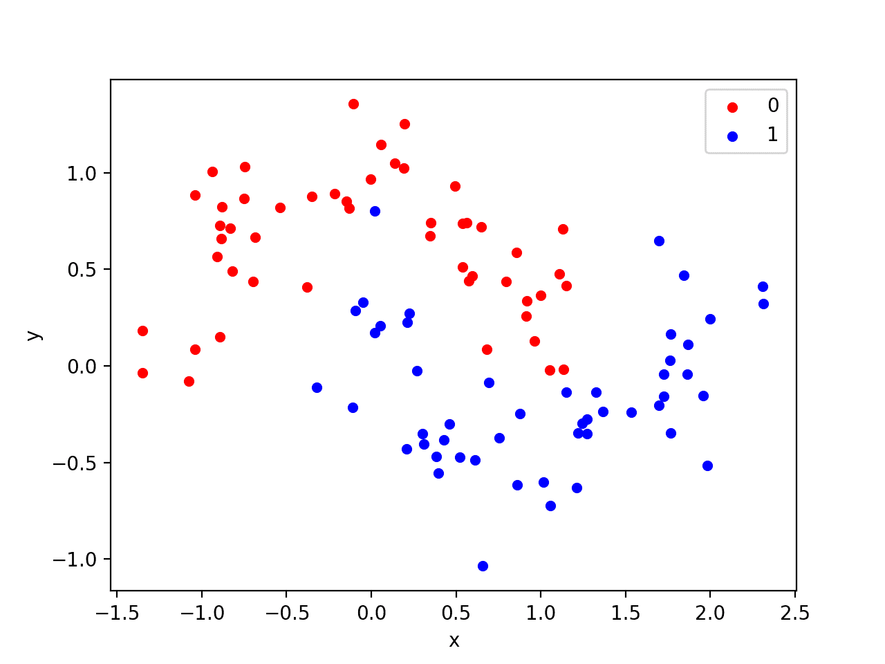
We will use a standard binary classification problem that defines two semi-circles of observations: one semi-circle for each class.
Each observation has two input variables with the same scale and a class output value of either 0 or 1. This dataset is called the “moons” dataset because of the shape of the observations in each class when plotted.
We can use the make_moons() function to generate observations from this problem. We will add noise to the data and seed the random number generator so that the same samples are generated each time the code is run.
We can plot the dataset where the two variables are taken as x and y coordinates on a graph and the class value is taken as the color of the observation.
The complete example of generating the dataset and plotting it is listed below.
Running the example creates a scatter plot showing the semi-circle or moon shape of the observations in each class. We can see the noise in the dispersal of the points making the moons less obvious.
Scatter Plot of Moons Dataset With Color Showing the Class Value of Each Sample
This is a good test problem because the classes cannot be separated by a line, e.g. are not linearly separable, requiring a nonlinear method such as a neural network to address.
We have only generated 100 samples, which is small for a neural network, providing the opportunity to overfit the training dataset and have higher error on the test dataset: a good case for using regularization. Further, the samples have noise, giving the model an opportunity to learn aspects of the samples that don’t generalize.
Overfit Multilayer Perceptron Model
We can develop an MLP model to address this binary classification problem.
The model will have one hidden layer with more nodes that may be required to solve this problem, providing an opportunity to overfit. We will also train the model for longer than is required to ensure the model overfits.
Before we define the model, we will split the dataset into train and test sets, using 30 examples to train the model and 70 to evaluate the fit model’s performance.
The model uses 500 nodes in the hidden layer and the rectified linear activation function.
A sigmoid activation function is used in the output layer in order to predict class values of 0 or 1.
The model is optimized using the binary cross entropy loss function, suitable for binary classification problems and the efficient Adam version of gradient descent.
Running the example reports the model performance on the train and test datasets.
We can see that the model has better performance on the training dataset than the test dataset, one possible sign of overfitting.
Note: Your results may vary given the stochastic nature of the algorithm or evaluation procedure, or differences in numerical precision. Consider running the example a few times and compare the average outcome.
Because the model is severely overfit, we generally would not expect much, if any, variance in the accuracy across repeated runs of the model on the same dataset.
1
Train: 1.000, Test: 0.914
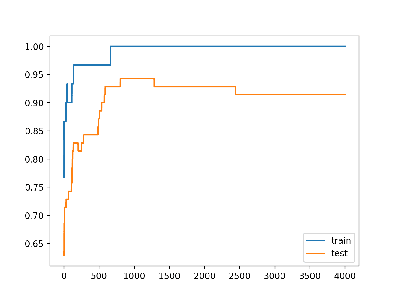
Another sign of overfitting is a plot of the learning curves of the model for both train and test datasets while training.
An overfit model should show accuracy increasing on both train and test and at some point accuracy drops on the test dataset but continues to rise on the training dataset.
We can update the example to plot these curves. The complete example is listed below.
1
2
3
4
5
6
7
8
9
10
11
12
13
14
15
16
17
18
19
20
21
22
23
24
# overfit mlp for the moons dataset plotting history
Running the example creates line plots of the model accuracy on the train and test sets.
We can see an expected shape of an overfit model where test accuracy increases to a point and then begins to decrease again.
Line Plots of Accuracy on Train and Test Datasets While Training
MLP Model With Weight Regularization
We can add weight regularization to the hidden layer to reduce the overfitting of the model to the training dataset and improve the performance on the holdout set.
We will use the L2 vector norm also called weight decay with a regularization parameter (called alpha or lambda) of 0.001, chosen arbitrarily.
This can be done by adding the kernel_regularizer argument to the layer and setting it to an instance of l2.
Running the example reports the performance of the model on the train and test datasets.
Note: Your results may vary given the stochastic nature of the algorithm or evaluation procedure, or differences in numerical precision. Consider running the example a few times and compare the average outcome.
We can see no change in the accuracy on the training dataset and an improvement on the test dataset.
1
Train: 1.000, Test: 0.943
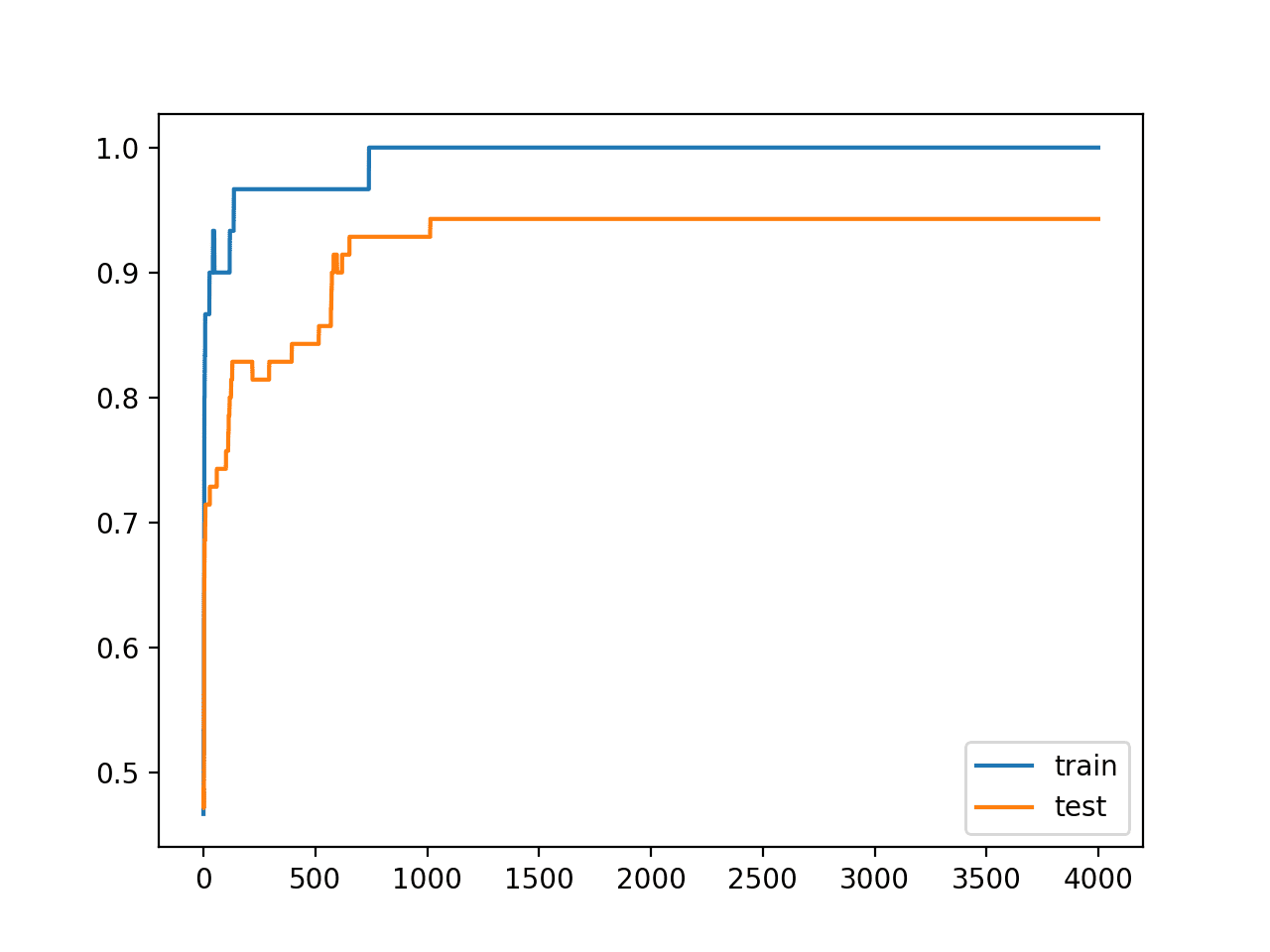
We would expect that the telltale learning curve for overfitting would also have been changed through the use of weight regularization.
Instead of the accuracy of the model on the test set increasing and then decreasing again, we should see it continually rise during training.
The complete example of fitting the model and plotting the train and test learning curves is listed below.
1
2
3
4
5
6
7
8
9
10
11
12
13
14
15
16
17
18
19
20
21
22
23
24
25
# mlp with weight regularization for the moons dataset plotting history
Running the example creates line plots of the train and test accuracy for the model for each epoch during training.
As expected, we see the learning curve on the test dataset rise and then plateau, indicating that the model may not have overfit the training dataset.
Line Plots of Accuracy on Train and Test Datasets While Training Without Overfitting
Grid Search Regularization Hyperparameter
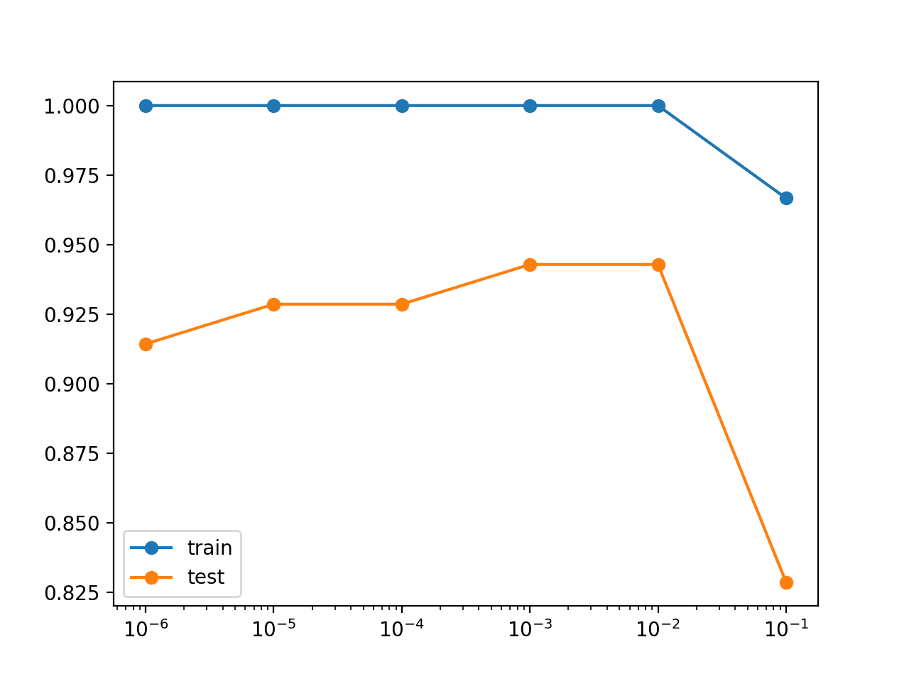
Once you can confirm that weight regularization may improve your overfit model, you can test different values of the regularization parameter.
It is a good practice to first grid search through some orders of magnitude between 0.0 and 0.1, then once a level is found, to grid search on that level.
We can grid search through the orders of magnitude by defining the values to test, looping through each and recording the train and test performance.
Once we have all of the values, we can graph the results as a line plot to help spot any patterns in the configurations to the train and test accuracies.
Because parameters jump orders of magnitude (powers of 10), we can create a line plot of the results using a logarithmic scale. The Matplotlib library allows this via the semilogx() function. For example:
Running the example prints the parameter value and the accuracy on the train and test sets for each evaluated model.
Note: Your results may vary given the stochastic nature of the algorithm or evaluation procedure, or differences in numerical precision. Consider running the example a few times and compare the average outcome.
The results suggest that 0.01 or 0.001 may be sufficient and may provide good bounds for further grid searching.
1
2
3
4
5
6
Param: 0.100000, Train: 0.967, Test: 0.829
Param: 0.010000, Train: 1.000, Test: 0.943
Param: 0.001000, Train: 1.000, Test: 0.943
Param: 0.000100, Train: 1.000, Test: 0.929
Param: 0.000010, Train: 1.000, Test: 0.929
Param: 0.000001, Train: 1.000, Test: 0.914
A line plot of the results is also created, showing the increase in test accuracy with larger weight regularization parameter values, at least to a point.
We can see that using the largest value of 0.1 results in a large drop in both train and test accuracy.
Line Plot of Model Accuracy on Train and Test Datasets With Different Weight Regularization Parameters
Extensions
This section lists some ideas for extending the tutorial that you may wish to explore.
Try Alternates. Update the example to use L1 or the combined L1L2 methods instead of L2 regularization.
Report Weight Norm. Update the example to calculate the magnitude of the network weights and demonstrate that regularization indeed made the magnitude smaller.
Regularize Output Layer. Update the example to regularize the output layer of the model and compare the results.
Regularize Bias. Update the example to regularize the bias weight and compare the results.
Repeated Model Evaluation. Update the example to fit and evaluate the model multiple times and report the mean and standard deviation of model performance.
Grid Search Along Order of Magnitude. Update the grid search example to grid search within the best-performing order of magnitude of parameter values.
Repeated Regularization of Model. Create a new example to continue the training of a fit model with increasing levels of regularization (e.g. 1E-6, 1E-5, etc.) and see if it results in a better performing model on the test set.
If you explore any of these extensions, I’d love to know.
Further Reading
This section provides more resources on the topic if you are looking to go deeper.
In this tutorial, you discovered how to apply weight regularization to improve the performance of an overfit deep learning neural network in Python with Keras.
Specifically, you learned:
How to use Keras API to add weight regularization to an MLP, CNN, or LSTM neural network.
Examples of weight regularization configurations used in books and recent research papers.
How to work through a case study for identifying an overfit model and improving test performance using weight regularization.
Do you have any questions?
Ask your questions in the comments below and I will do my best to answer.
– I already finished this nice weigh regularization case study with MLP neural model and using make_moons function from sklearn library as the dataset generator. Thank you. Very clear exercise and I could reproduce exactly all yours output numbers !.
– Regarding some extension of this exercise, as you mention in the beginning that the LSTM and CNN models types also accept keras regularizers, such as l1, l2, l1_l2…I was wondering how could we implement another case study using the same make_moons function but now with LSTM and/or CNN model?
Just adding a new Convolutional 2D layer (plus the maxpool layer plus flatten layer I guess) before the dense layer of your code? and what about LSTM, just switching directly the dense layer line code by a new regularized LSTM layer? or probably it is more complex and does not work for this moons dataset exercise? It could be convenient if someone could write down these few lines of CNN and/or LSTM model definition of code, if it is thinking helpful…
CNN and LSTM would not be appropriate for the moons problem. They would require a sequence prediction problem. You could contrive a small sequence prediction problem for testing.
In addition to the previous question, about CNN/LST regularizer code implementation I will be grateful if you can provide us with some rule -recommendation (if anyone exist?) about:
– how to implement regularizers in several model layers, in the sense of:
do I have to set strong weight decay (e.g. higher L2 values) in the first layers (the ones that generalize better the problem solution) and weaker weight decay (e.g. lower L2 values) on the last model ayers (the ones more abstracts) ? or vice versa (the opposite way)?
My intuition will suggest me to try higher attenuations (strong weight decay) in the first layers (the ones that generalize better) and lower attenuation (smoother decay) in the last ones (the abstracts layers)….
Also because from the point of view of model instability (output response to input in term of convergence), the model it is more sensible to first layers weight values (so bigger ones will produce more instability)…But all of this are intuitions ideas not confirmed yet…What do you think Jason?
From what I have seen, the same level of weight regularization is used across all layers. Perhaps try experimenting with different approaches to see if it makes a difference.
Comparison of Human vs. Machine-learning:
It is of great interest to know whether human perception is important in identifying spoofing and hence, humans can achieve better performance than automatic approaches in detecting spoofing attacks. There was a benchmark study that compared automatic systems against human performance on a speaker verification and synthetic speech spoofing detection tasks (SS and VC spoofs). It was observed that human listeners detect spoofing less well than most of the automatic approaches except USS speech. In a similar study, it was found that both the humans and machines have difficulties in spoofing detection when narrowband speech signals were used (8 kHz sampling frequency). Hence, for telephone line speech signals, it is more challenging to do SSD due to the lower available bandwidth up to 4 kHz. It may be of great interest to study human performance for replay SSD task.
Great article Jason!! Thanks for the insights… Is there a way of extracting feature importance from the CNN model? Please provide some pointers or link to an article you have published on these lines.
Thanks Dr Jason for the most helpful topics. your tutorials help me to increase my model accuracy from 60% to 95%.
you explain every thing very clear and that’s great for people whose native language is not English. Like me from Afghanistan
Well that was an amazing article Jason.
One thing I wanted to ask.. do you have any idea how l2-l1 is different from dropout layers in reducing overfitting?
“An overfit model should show accuracy increasing on both train and test and at some point accuracy drops on the test dataset but continues to rise on the test dataset.”
There is a mistake in this line last word should be train dataset.
in my case, when I have the situation of overfitting, I add some weight regularization to dense layer, then the loss of the training data will increase (R squared score decrease), but the loss of the validation data does not improve (R squared keeps no big change), finally both loss of validation data and training data are similar, but both are high.
is it normal? How to handle this situation please?
Thank you.
Firstly, thank you very much for this tutorial. It is indeed so helpful.
Secondly, I want to point out for something, while plotting the history (of the losses/accuracies), the x-axis shall start from “1” and not “0” if I am correct. Since the evaluation is only occuring at the end of each epoch.
What this article means is the regularization based on weight, surely we can do that using L2 with Adam. The article you referred saying the L2 regularization (which has a strict definition in formula) is same as weight decay (which is more a concept than an exact algorithm) are the same formula according to the author.
Dear Mr.Jason,
I’m once again referring to your cool articles 🙂
I have some sort of a weird question..
Can we include more than one regularization layer in a model as in below? I’m wondering whether something like this is possible.. Could you please let me know your thoughts on this?


Hola Jason,
– I already finished this nice weigh regularization case study with MLP neural model and using make_moons function from sklearn library as the dataset generator. Thank you. Very clear exercise and I could reproduce exactly all yours output numbers !.
– Regarding some extension of this exercise, as you mention in the beginning that the LSTM and CNN models types also accept keras regularizers, such as l1, l2, l1_l2…I was wondering how could we implement another case study using the same make_moons function but now with LSTM and/or CNN model?
Just adding a new Convolutional 2D layer (plus the maxpool layer plus flatten layer I guess) before the dense layer of your code? and what about LSTM, just switching directly the dense layer line code by a new regularized LSTM layer? or probably it is more complex and does not work for this moons dataset exercise? It could be convenient if someone could write down these few lines of CNN and/or LSTM model definition of code, if it is thinking helpful…
thanks
Thanks, well done!
CNN and LSTM would not be appropriate for the moons problem. They would require a sequence prediction problem. You could contrive a small sequence prediction problem for testing.
In addition to the previous question, about CNN/LST regularizer code implementation I will be grateful if you can provide us with some rule -recommendation (if anyone exist?) about:
– how to implement regularizers in several model layers, in the sense of:
do I have to set strong weight decay (e.g. higher L2 values) in the first layers (the ones that generalize better the problem solution) and weaker weight decay (e.g. lower L2 values) on the last model ayers (the ones more abstracts) ? or vice versa (the opposite way)?
My intuition will suggest me to try higher attenuations (strong weight decay) in the first layers (the ones that generalize better) and lower attenuation (smoother decay) in the last ones (the abstracts layers)….
Also because from the point of view of model instability (output response to input in term of convergence), the model it is more sensible to first layers weight values (so bigger ones will produce more instability)…But all of this are intuitions ideas not confirmed yet…What do you think Jason?
From what I have seen, the same level of weight regularization is used across all layers. Perhaps try experimenting with different approaches to see if it makes a difference.
Comparison of Human vs. Machine-learning:
It is of great interest to know whether human perception is important in identifying spoofing and hence, humans can achieve better performance than automatic approaches in detecting spoofing attacks. There was a benchmark study that compared automatic systems against human performance on a speaker verification and synthetic speech spoofing detection tasks (SS and VC spoofs). It was observed that human listeners detect spoofing less well than most of the automatic approaches except USS speech. In a similar study, it was found that both the humans and machines have difficulties in spoofing detection when narrowband speech signals were used (8 kHz sampling frequency). Hence, for telephone line speech signals, it is more challenging to do SSD due to the lower available bandwidth up to 4 kHz. It may be of great interest to study human performance for replay SSD task.
Intersting, thanks for sharing.
Great article Jason!! Thanks for the insights… Is there a way of extracting feature importance from the CNN model? Please provide some pointers or link to an article you have published on these lines.
Best Regards
Sowmya
Perhaps. I don’t have an example sorry.
Great writing ! Look forward to similar teaching on reinforcement learning !
Thanks !
Yong
Thanks.
Thanks Dr Jason for the most helpful topics. your tutorials help me to increase my model accuracy from 60% to 95%.
you explain every thing very clear and that’s great for people whose native language is not English. Like me from Afghanistan
Well done!
Thanks, I’m happy to hear that.
Well that was an amazing article Jason.
One thing I wanted to ask.. do you have any idea how l2-l1 is different from dropout layers in reducing overfitting?
Thanks,
Best Regards,
Abhilash Mandal
Thanks!
Yes, vector norms keep the weights small and the model stable/general. Dropout forces other nodes in the layer to generalize.
“An overfit model should show accuracy increasing on both train and test and at some point accuracy drops on the test dataset but continues to rise on the test dataset.”
There is a mistake in this line last word should be train dataset.
BTW,
You are doing an amazing job. 😀
Thanks, fixed!
Hi Jason,
in my case, when I have the situation of overfitting, I add some weight regularization to dense layer, then the loss of the training data will increase (R squared score decrease), but the loss of the validation data does not improve (R squared keeps no big change), finally both loss of validation data and training data are similar, but both are high.
is it normal? How to handle this situation please?
Thank you.
Perhaps try an alternate regularization method:
https://machinelearningmastery.com/introduction-to-regularization-to-reduce-overfitting-and-improve-generalization-error/
Firstly, thank you very much for this tutorial. It is indeed so helpful.
Secondly, I want to point out for something, while plotting the history (of the losses/accuracies), the x-axis shall start from “1” and not “0” if I am correct. Since the evaluation is only occuring at the end of each epoch.
Sure.
hi,
the recurrent regularizer is referent to the weight between an lstm memory cell and the one after it?
Weight decay will drive the weights in the model smaller during training. This applies to LSTMs, CNNs, and MLPs.
Is weight decay == L2 regularization in keras?
Yes.
I really appreciate the work you put into these…
One question though: here (https://www.fast.ai/2018/07/02/adam-weight-decay/#understanding-adamw-weight-decay-or-l2-regularization) it says that weight decay and L2 regularization are only the same for plain SGD, yet you are using adam with L2 regularization and calling it weight decay, IIUC – can you clarify?
What this article means is the regularization based on weight, surely we can do that using L2 with Adam. The article you referred saying the L2 regularization (which has a strict definition in formula) is same as weight decay (which is more a concept than an exact algorithm) are the same formula according to the author.
Dear Mr.Jason,
I’m once again referring to your cool articles 🙂
I have some sort of a weird question..
Can we include more than one regularization layer in a model as in below? I’m wondering whether something like this is possible.. Could you please let me know your thoughts on this?
model = keras.Sequential([
layers.Dense(20, activation=’relu’),
layers.Dropout(0.3),
layers.BatchNormalization(),
layers.Dense(10, kernel_regularizer=regularizers.L2(l2=0.01)),
layers.Dense(20, activation=’relu’),
layers.Dense(10, kernel_regularizer=regularizers.L2(l2=0.01)),
layers.Dense(2, activation=’sigmoid’),
])
Not Jason here, but yes.
I believe that the research models referenced should use regularization in most to all of their layers, but correct me if I’m wrong.