How to Reduce Overfitting Using Weight Constraints in Keras

Weight constraints provide an approach to reduce the overfitting of a deep learning neural network model on the training data and improve the performance of the model on new data, such as the holdout test set.

There are multiple types of weight constraints, such as maximum and unit vector norms, and some require a hyperparameter that must be configured.

In this tutorial, you will discover the Keras API for adding weight constraints to deep learning neural network models to reduce overfitting.

After completing this tutorial, you will know:

• How to create vector norm constraints using the Keras API.
• How to add weight constraints to MLP, CNN, and RNN layers using the Keras API.
• How to reduce overfitting by adding a weight constraint to an existing model.

Kick-start your project with my new book Better Deep Learning, including step-by-step tutorials and the Python source code files for all examples.

Let’s get started.

• Updated Mar/2019: fixed typo using equality instead of assignment in some usage examples.
• Updated Oct/2019: Updated for Keras 2.3 and TensorFlow 2.0.

How to Reduce Overfitting in Deep Neural Networks With Weight Constraints in Keras
Photo by Ian Sane, some rights reserved.

Tutorial Overview

This tutorial is divided into three parts; they are:

1. Weight Constraints in Keras
2. Weight Constraints on Layers
3. Weight Constraint Case Study

Weight Constraints in Keras

The Keras API supports weight constraints.

The constraints are specified per-layer, but applied and enforced per-node within the layer.

Using a constraint generally involves setting the kernel_constraint argument on the layer for the input weights and the bias_constraint for the bias weights.

Generally, weight constraints are not used on the bias weights.

A suite of different vector norms can be used as constraints, provided as classes in the keras.constraints module. They are:

• Maximum norm (max_norm), to force weights to have a magnitude at or below a given limit.
• Non-negative norm (non_neg), to force weights to have a positive magnitude.
• Unit norm (unit_norm), to force weights to have a magnitude of 1.0.
• Min-Max norm (min_max_norm), to force weights to have a magnitude between a range.

For example, a constraint can imported and instantiated:

Weight Constraints on Layers

The weight norms can be used with most layers in Keras.

In this section, we will look at some common examples.

MLP Weight Constraint

The example below sets a maximum norm weight constraint on a Dense fully connected layer.

CNN Weight Constraint

The example below sets a maximum norm weight constraint on a convolutional layer.

RNN Weight Constraint

Unlike other layer types, recurrent neural networks allow you to set a weight constraint on both the input weights and bias, as well as the recurrent input weights.

The constraint for the recurrent weights is set via the recurrent_constraint argument to the layer.

The example below sets a maximum norm weight constraint on an LSTM layer.

Now that we know how to use the weight constraint API, let’s look at a worked example.

Weight Constraint Case Study

In this section, we will demonstrate how to use weight constraints to reduce overfitting of an MLP on a simple binary classification problem.

This example provides a template for applying weight constraints to your own neural network for classification and regression problems.

Binary Classification Problem

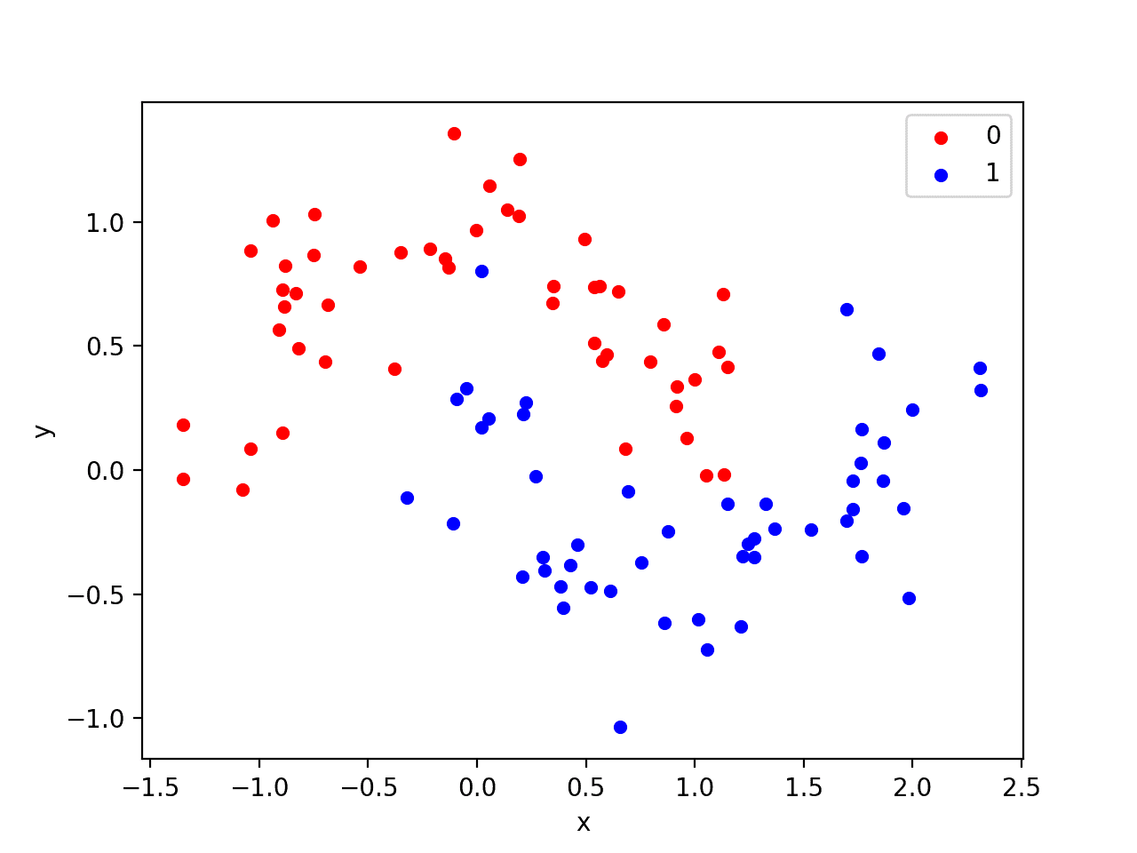
We will use a standard binary classification problem that defines two semi-circles of observations, one semi-circle for each class.

Each observation has two input variables with the same scale and a class output value of either 0 or 1. This dataset is called the “moons” dataset because of the shape of the observations in each class when plotted.

We can use the make_moons() function to generate observations from this problem. We will add noise to the data and seed the random number generator so that the same samples are generated each time the code is run.

We can plot the dataset where the two variables are taken as x and y coordinates on a graph and the class value is taken as the color of the observation.

The complete example of generating the dataset and plotting it is listed below.

Running the example creates a scatter plot showing the semi-circle or moon shape of the observations in each class. We can see the noise in the dispersal of the points making the moons less obvious.

Scatter Plot of Moons Dataset With Color Showing the Class Value of Each Sample

This is a good test problem because the classes cannot be separated by a line, e.g. are not linearly separable, requiring a nonlinear method such as a neural network to address.

We have only generated 100 samples, which is small for a neural network, providing the opportunity to overfit the training dataset and have higher error on the test dataset: a good case for using regularization. Further, the samples have noise, giving the model an opportunity to learn aspects of the samples that don’t generalize.

Overfit Multilayer Perceptron

We can develop an MLP model to address this binary classification problem.

The model will have one hidden layer with more nodes than may be required to solve this problem, providing an opportunity to overfit. We will also train the model for longer than is required to ensure the model overfits.

Before we define the model, we will split the dataset into train and test sets, using 30 examples to train the model and 70 to evaluate the fit model’s performance.

Next, we can define the model.

The hidden layer uses 500 nodes in the hidden layer and the rectified linear activation function. A sigmoid activation function is used in the output layer in order to predict class values of 0 or 1.

The model is optimized using the binary cross entropy loss function, suitable for binary classification problems and the efficient Adam version of gradient descent.

The defined model is then fit on the training data for 4,000 epochs and the default batch size of 32.

We will also use the test dataset as a validation dataset.

We can evaluate the performance of the model on the test dataset and report the result.

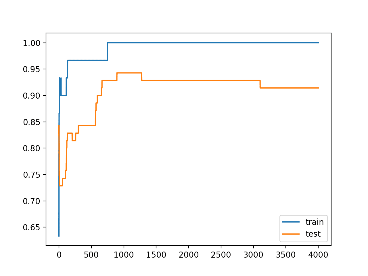
Finally, we will plot the performance of the model on both the train and test set each epoch.

If the model does indeed overfit the training dataset, we would expect the line plot of accuracy on the training set to continue to increase and the test set to rise and then fall again as the model learns statistical noise in the training dataset.

We can tie all of these pieces together; the complete example is listed below.

Running the example reports the model performance on the train and test datasets.

We can see that the model has better performance on the training dataset than the test dataset, one possible sign of overfitting.

Note: Your results may vary given the stochastic nature of the algorithm or evaluation procedure, or differences in numerical precision. Consider running the example a few times and compare the average outcome.

Because the model is overfit, we generally would not expect much, if any, variance in the accuracy across repeated runs of the model on the same dataset.

A figure is created showing line plots of the model accuracy on the train and test sets.

We can see that expected shape of an overfit model where test accuracy increases to a point and then begins to decrease again.

Line Plots of Accuracy on Train and Test Datasets While Training Showing an Overfit

Overfit MLP With Weight Constraint

We can update the example to use a weight constraint.

There are a few different weight constraints to choose from. A good simple constraint for this model is to simply normalize the weights so that the norm is equal to 1.0.

This constraint has the effect of forcing all incoming weights to be small.

We can do this by using the unit_norm in Keras. This constraint can be added to the first hidden layer as follows:

We can also achieve the same result by using the min_max_norm and setting the min and maximum to 1.0, for example:

We cannot achieve the same result with the maximum norm constraint as it will allow norms at or below the specified limit; for example:

The complete updated example with the unit norm constraint is listed below:

Running the example reports the model performance on the train and test datasets.

Note: Your results may vary given the stochastic nature of the algorithm or evaluation procedure, or differences in numerical precision. Consider running the example a few times and compare the average outcome.

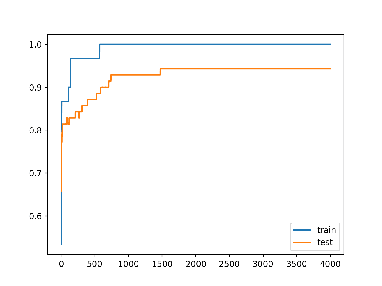
We can see that indeed the strict constraint on the size of the weights has improved the performance of the model on the holdout set without impacting performance on the training set.

Reviewing the line plot of train and test accuracy, we can see that it no longer appears that the model has overfit the training dataset.

Model accuracy on both the train and test sets continues to increase to a plateau.

Line Plots of Accuracy on Train and Test Datasets While Training With Weight Constraints

Extensions

This section lists some ideas for extending the tutorial that you may wish to explore.

• Report Weight Norm. Update the example to calculate the magnitude of the network weights and demonstrate that the constraint indeed made the magnitude smaller.
• Constrain Output Layer. Update the example to add a constraint to the output layer of the model and compare the results.
• Constrain Bias. Update the example to add a constraint to the bias weight and compare the results.
• Repeated Evaluation. Update the example to fit and evaluate the model multiple times and report the mean and standard deviation of model performance.

If you explore any of these extensions, I’d love to know.

Further Reading

This section provides more resources on the topic if you are looking to go deeper.

Posts

• Gentle Introduction to Vector Norms in Machine Learning

API

• Keras Constraints API
• Keras constraints.py
• Keras Core Layers API
• Keras Convolutional Layers API
• Keras Recurrent Layers API
• sklearn.datasets.make_moons API

Summary

In this tutorial, you discovered the Keras API for adding weight constraints to deep learning neural network models.

Specifically, you learned:

• How to create vector norm constraints using the Keras API.
• How to add weight constraints to MLP, CNN, and RNN layers using the Keras API.
• How to reduce overfitting by adding a weight constraint to an existing model.

Do you have any questions?
Ask your questions in the comments below and I will do my best to answer.

Develop Better Deep Learning Models Today!

Train Faster, Reduce Overftting, and Ensembles

...with just a few lines of python code

Discover how in my new Ebook:
Better Deep Learning

It provides self-study tutorials on topics like:
weight decay, batch normalization, dropout, model stacking and much more...

Bring better deep learning to your projects!

Skip the Academics. Just Results.

See What's Inside