Deep Learning for Computer Vision Crash Course.
Bring Deep Learning Methods to Your Computer Vision Project in 7 Days.
We are awash in digital images from photos, videos, Instagram, YouTube, and increasingly live video streams.
Working with image data is hard as it requires drawing upon knowledge from diverse domains such as digital signal processing, machine learning, statistical methods, and these days, deep learning.
Deep learning methods are out-competing the classical and statistical methods on some challenging computer vision problems with singular and simpler models.
In this crash course, you will discover how you can get started and confidently develop deep learning for computer vision problems using Python in seven days.
Note: This is a big and important post. You might want to bookmark it.
Let’s get started.
- Update Nov/2019: Updated for TensorFlow v2.0 and MTCNN v0.1.0.

How to Get Started With Deep Learning for Computer Vision (7-Day Mini-Course)
Photo by oliver.dodd, some rights reserved.
Who Is This Crash-Course For?
Before we get started, let’s make sure you are in the right place.
The list below provides some general guidelines as to who this course was designed for.
Don’t panic if you don’t match these points exactly; you might just need to brush up in one area or another to keep up.
You need to know:
- You need to know your way around basic Python, NumPy, and Keras for deep learning.
You do NOT need to be:
- You do not need to be a math wiz!
- You do not need to be a deep learning expert!
- You do not need to be a computer vision researcher!
This crash course will take you from a developer that knows a little machine learning to a developer who can bring deep learning methods to your own computer vision project.
Note: This crash course assumes you have a working Python 2 or 3 SciPy environment with at least NumPy, Pandas, scikit-learn, and Keras 2 installed. If you need help with your environment, you can follow the step-by-step tutorial here:
Crash-Course Overview
This crash course is broken down into seven lessons.
You could complete one lesson per day (recommended) or complete all of the lessons in one day (hardcore). It really depends on the time you have available and your level of enthusiasm.
Below are the seven lessons that will get you started and productive with deep learning for computer vision in Python:
- Lesson 01: Deep Learning and Computer Vision
- Lesson 02: Preparing Image Data
- Lesson 03: Convolutional Neural Networks
- Lesson 04: Image Classification
- Lesson 05: Train Image Classification Model
- Lesson 06: Image Augmentation
- Lesson 07: Face Detection
Each lesson could take you anywhere from 60 seconds up to 30 minutes. Take your time and complete the lessons at your own pace. Ask questions and even post results in the comments below.
The lessons might expect you to go off and find out how to do things. I will give you hints, but part of the point of each lesson is to force you to learn where to go to look for help on and about the deep learning, computer vision, and the best-of-breed tools in Python (hint: I have all of the answers on this blog, just use the search box).
Post your results in the comments; I’ll cheer you on!
Hang in there; don’t give up.
Note: This is just a crash course. For a lot more detail and fleshed out tutorials, see my book on the topic titled “Deep Learning for Computer Vision.”
Want Results with Deep Learning for Computer Vision?
Take my free 7-day email crash course now (with sample code).
Click to sign-up and also get a free PDF Ebook version of the course.
Lesson 01: Deep Learning and Computer Vision
In this lesson, you will discover the promise of deep learning methods for computer vision.
Computer Vision
Computer Vision, or CV for short, is broadly defined as helping computers to “see” or extract meaning from digital images such as photographs and videos.
Researchers have been working on the problem of helping computers see for more than 50 years, and some great successes have been achieved, such as the face detection available in modern cameras and smartphones.
The problem of understanding images is not solved, and may never be. This is primarily because the world is complex and messy. There are few rules. And yet we can easily and effortlessly recognize objects, people, and context.
Deep Learning
Deep Learning is a subfield of machine learning concerned with algorithms inspired by the structure and function of the brain called artificial neural networks.
A property of deep learning is that the performance of this type of model improves by training it with more examples and by increasing its depth or representational capacity.
In addition to scalability, another often-cited benefit of deep learning models is their ability to perform automatic feature extraction from raw data, also called feature learning.
Promise of Deep Learning for Computer vision
Deep learning methods are popular for computer vision, primarily because they are delivering on their promise.
Some of the first large demonstrations of the power of deep learning were in computer vision, specifically image classification. More recently in object detection and face recognition.
The three key promises of deep learning for computer vision are as follows:
- The Promise of Feature Learning. That is, that deep learning methods can automatically learn the features from image data required by the model, rather than requiring that the feature detectors be handcrafted and specified by an expert.
- The Promise of Continued Improvement. That is, that the performance of deep learning in computer vision is based on real results and that the improvements appear to be continuing and perhaps speeding up.
- The Promise of End-to-End Models. That is, that large end-to-end deep learning models can be fit on large datasets of images or video offering a more general and better-performing approach.
Computer vision is not “solved” but deep learning is required to get you to the state-of-the-art on many challenging problems in the field.
Your Task
For this lesson, you must research and list five impressive applications of deep learning methods in the field of computer vision. Bonus points if you can link to a research paper that demonstrates the example.
Post your answer in the comments below. I would love to see what you discover.
In the next lesson, you will discover how to prepare image data for modeling.
Lesson 02: Preparing Image Data
In this lesson, you will discover how to prepare image data for modeling.
Images are comprised of matrices of pixel values.
Pixel values are often unsigned integers in the range between 0 and 255. Although these pixel values can be presented directly to neural network models in their raw format, this can result in challenges during modeling, such as slower than expected training of the model.
Instead, there can be great benefit in preparing the image pixel values prior to modeling, such as simply scaling pixel values to the range 0-1 to centering and even standardizing the values.
This is called normalization and can be performed directly on a loaded image. The example below uses the PIL library (the standard image handling library in Python) to load an image and normalize its pixel values.
First, confirm that you have the Pillow library installed; it is installed with most SciPy environments, but you can learn more here:
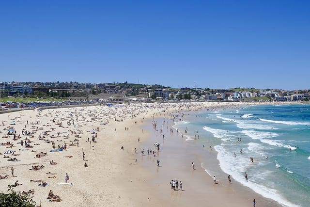
Next, download a photograph of Bondi Beach in Sydney Australia, taken by Isabell Schulz and released under a permissive license. Save the image in your current working directory with the filename ‘bondi_beach.jpg‘.
Next, we can use the Pillow library to load the photo, confirm the min and max pixel values, normalize the values, and confirm the normalization was performed.
|
1 2 3 4 5 6 7 8 9 10 11 12 13 14 15 |
# example of pixel normalization from numpy import asarray from PIL import Image # load image image = Image.open('bondi_beach.jpg') pixels = asarray(image) # confirm pixel range is 0-255 print('Data Type: %s' % pixels.dtype) print('Min: %.3f, Max: %.3f' % (pixels.min(), pixels.max())) # convert from integers to floats pixels = pixels.astype('float32') # normalize to the range 0-1 pixels /= 255.0 # confirm the normalization print('Min: %.3f, Max: %.3f' % (pixels.min(), pixels.max())) |
Your Task
Your task in this lesson is to run the example code on the provided photograph and report the min and max pixel values before and after the normalization.
For bonus points, you can update the example to standardize the pixel values.
Post your findings in the comments below. I would love to see what you discover.
In the next lesson, you will discover information about convolutional neural network models.
Lesson 03: Convolutional Neural Networks
In this lesson, you will discover how to construct a convolutional neural network using a convolutional layer, pooling layer, and fully connected output layer.
Convolutional Layers
A convolution is the simple application of a filter to an input that results in an activation. Repeated application of the same filter to an input results in a map of activations called a feature map, indicating the locations and strength of a detected feature in an input, such as an image.
A convolutional layer can be created by specifying both the number of filters to learn and the fixed size of each filter, often called the kernel shape.
Pooling Layers
Pooling layers provide an approach to downsampling feature maps by summarizing the presence of features in patches of the feature map.
Maximum pooling, or max pooling, is a pooling operation that calculates the maximum, or largest, value in each patch of each feature map.
Classifier Layer
Once the features have been extracted, they can be interpreted and used to make a prediction, such as classifying the type of object in a photograph.
This can be achieved by first flattening the two-dimensional feature maps, and then adding a fully connected output layer. For a binary classification problem, the output layer would have one node that would predict a value between 0 and 1 for the two classes.
Convolutional Neural Network
The example below creates a convolutional neural network that expects grayscale images with the square size of 256×256 pixels, with one convolutional layer with 32 filters, each with the size of 3×3 pixels, a max pooling layer, and a binary classification output layer.
|
1 2 3 4 5 6 7 8 9 10 11 12 13 14 |
# cnn with single convolutional, pooling and output layer from keras.models import Sequential from keras.layers import Conv2D from keras.layers import MaxPooling2D from keras.layers import Flatten from keras.layers import Dense # create model model = Sequential() # add convolutional layer model.add(Conv2D(32, (3,3), input_shape=(256, 256, 1))) model.add(MaxPooling2D()) model.add(Flatten()) model.add(Dense(1, activation='sigmoid')) model.summary() |
Your Task
Your task in this lesson is to run the example and describe how the shape of an input image would be changed by the convolutional and pooling layers.
For extra points, you could try adding more convolutional or pooling layers and describe the effect it has on the image as it flows through the model.
Post your findings in the comments below. I would love to see what you discover.
In the next lesson, you will learn how to use a deep convolutional neural network to classify photographs of objects.
Lesson 04: Image Classification
In this lesson, you will discover how to use a pre-trained model to classify photographs of objects.
Deep convolutional neural network models may take days, or even weeks, to train on very large datasets.
A way to short-cut this process is to re-use the model weights from pre-trained models that were developed for standard computer vision benchmark datasets, such as the ImageNet image recognition tasks.
The example below uses the VGG-16 pre-trained model to classify photographs of objects into one of 1,000 known classes.
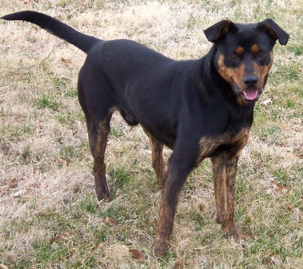
Download this photograph of a dog taken by Justin Morgan and released under a permissive license. Save it in your current working directory with the filename ‘dog.jpg‘.
The example below will load the photograph and output a prediction, classifying the object in the photograph.
Note: The first time you run the example, the pre-trained model will have to be downloaded, which is a few hundred megabytes and make take a few minutes based on the speed of your internet connection.
|
1 2 3 4 5 6 7 8 9 10 11 12 13 14 15 16 17 18 19 20 21 22 23 24 |
# example of using a pre-trained model as a classifier from keras.preprocessing.image import load_img from keras.preprocessing.image import img_to_array from keras.applications.vgg16 import preprocess_input from keras.applications.vgg16 import decode_predictions from keras.applications.vgg16 import VGG16 # load an image from file image = load_img('dog.jpg', target_size=(224, 224)) # convert the image pixels to a numpy array image = img_to_array(image) # reshape data for the model image = image.reshape((1, image.shape[0], image.shape[1], image.shape[2])) # prepare the image for the VGG model image = preprocess_input(image) # load the model model = VGG16() # predict the probability across all output classes yhat = model.predict(image) # convert the probabilities to class labels label = decode_predictions(yhat) # retrieve the most likely result, e.g. highest probability label = label[0][0] # print the classification print('%s (%.2f%%)' % (label[1], label[2]*100)) |
Your Task
Your task in this lesson is to run the example and report the result.
For bonus points, try running the example on another photograph of a common object.
Post your findings in the comments below. I would love to see what you discover.
In the next lesson, you will discover how to fit and evaluate a model for image classification.
Lesson 05: Train Image Classification Model
In this lesson, you will discover how to train and evaluate a convolutional neural network for image classification.
The Fashion-MNIST clothing classification problem is a new standard dataset used in computer vision and deep learning.
It is a dataset comprised of 60,000 small square 28×28 pixel grayscale images of items of 10 types of clothing, such as shoes, t-shirts, dresses, and more.
The example below loads the dataset, scales the pixel values, then fits a convolutional neural network on the training dataset and evaluates the performance of the network on the test dataset.
The example will run in just a few minutes on a modern CPU; no GPU is required.
|
1 2 3 4 5 6 7 8 9 10 11 12 13 14 15 16 17 18 19 20 21 22 23 24 25 26 27 28 29 30 31 32 |
# fit a cnn on the fashion mnist dataset from keras.datasets import fashion_mnist from keras.utils import to_categorical from keras.models import Sequential from keras.layers import Conv2D from keras.layers import MaxPooling2D from keras.layers import Dense from keras.layers import Flatten # load dataset (trainX, trainY), (testX, testY) = fashion_mnist.load_data() # reshape dataset to have a single channel trainX = trainX.reshape((trainX.shape[0], 28, 28, 1)) testX = testX.reshape((testX.shape[0], 28, 28, 1)) # convert from integers to floats trainX, testX = trainX.astype('float32'), testX.astype('float32') # normalize to range 0-1 trainX,testX = trainX / 255.0, testX / 255.0 # one hot encode target values trainY, testY = to_categorical(trainY), to_categorical(testY) # define model model = Sequential() model.add(Conv2D(32, (3, 3), activation='relu', kernel_initializer='he_uniform', input_shape=(28, 28, 1))) model.add(MaxPooling2D()) model.add(Flatten()) model.add(Dense(100, activation='relu', kernel_initializer='he_uniform')) model.add(Dense(10, activation='softmax')) model.compile(optimizer='adam', loss='categorical_crossentropy', metrics=['accuracy']) # fit model model.fit(trainX, trainY, epochs=10, batch_size=32, verbose=2) # evaluate model loss, acc = model.evaluate(testX, testY, verbose=0) print(loss, acc) |
Your Task
Your task in this lesson is to run the example and report the performance of the model on the test dataset.
For bonus points, try varying the configuration of the model, or try saving the model and later loading it and using it to make a prediction on new grayscale photographs of clothing.
Post your findings in the comments below. I would love to see what you discover.
In the next lesson, you will discover how to use image augmentation on training data.
Lesson 06: Image Augmentation
In this lesson, you will discover how to use image augmentation.
Image data augmentation is a technique that can be used to artificially expand the size of a training dataset by creating modified versions of images in the dataset.
Training deep learning neural network models on more data can result in more skillful models, and the augmentation techniques can create variations of the images that can improve the ability of the fit models to generalize what they have learned to new images.
The Keras deep learning neural network library provides the capability to fit models using image data augmentation via the ImageDataGenerator class.
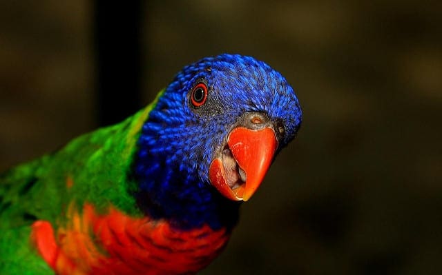
Download a photograph of a bird by AndYaDontStop, released under a permissive license. Save it into your current working directory with the name ‘bird.jpg‘.
The example below will load the photograph as a dataset and use image augmentation to create flipped and rotated versions of the image that can be used to train a convolutional neural network model.
|
1 2 3 4 5 6 7 8 9 10 11 12 13 14 15 16 17 18 19 20 21 22 23 24 25 26 27 28 |
# example using image augmentation from numpy import expand_dims from keras.preprocessing.image import load_img from keras.preprocessing.image import img_to_array from keras.preprocessing.image import ImageDataGenerator from matplotlib import pyplot # load the image img = load_img('bird.jpg') # convert to numpy array data = img_to_array(img) # expand dimension to one sample samples = expand_dims(data, 0) # create image data augmentation generator datagen = ImageDataGenerator(horizontal_flip=True, vertical_flip=True, rotation_range=90) # prepare iterator it = datagen.flow(samples, batch_size=1) # generate samples and plot for i in range(9): # define subplot pyplot.subplot(330 + 1 + i) # generate batch of images batch = it.next() # convert to unsigned integers for viewing image = batch[0].astype('uint32') # plot raw pixel data pyplot.imshow(image) # show the figure pyplot.show() |
Your Task
Your task in this lesson is to run the example and report the effect that the image augmentation has had on the original image.
For bonus points, try additional types of image augmentation, supported by the ImageDataGenerator class.
Post your findings in the comments below. I would love to see what you find.
In the next lesson, you will discover how to use a deep convolutional network to detect faces in photographs.
Lesson 07: Face Detection
In this lesson, you will discover how to use a convolutional neural network for face detection.
Face detection is a trivial problem for humans to solve and has been solved reasonably well by classical feature-based techniques, such as the cascade classifier.
More recently, deep learning methods have achieved state-of-the-art results on standard face detection datasets. One example is the Multi-task Cascade Convolutional Neural Network, or MTCNN for short.
The ipazc/MTCNN project provides an open source implementation of the MTCNN that can be installed easily as follows:
|
1 |
sudo pip install mtcnn |
Download a photograph of a person on the street taken by Holland and released under a permissive license. Save it into your current working directory with the name ‘street.jpg‘.
The example below will load the photograph and use the MTCNN model to detect faces and will plot the photo and draw a box around the first detected face.
|
1 2 3 4 5 6 7 8 9 10 11 12 13 14 15 16 17 18 19 20 21 22 |
# face detection with mtcnn on a photograph from matplotlib import pyplot from matplotlib.patches import Rectangle from mtcnn.mtcnn import MTCNN # load image from file pixels = pyplot.imread('street.jpg') # create the detector, using default weights detector = MTCNN() # detect faces in the image faces = detector.detect_faces(pixels) # plot the image pyplot.imshow(pixels) # get the context for drawing boxes ax = pyplot.gca() # get coordinates from the first face x, y, width, height = faces[0]['box'] # create the shape rect = Rectangle((x, y), width, height, fill=False, color='red') # draw the box ax.add_patch(rect) # show the plot pyplot.show() |
Your Task
Your task in this lesson is to run the example and describe the result.
For bonus points, try the model on another photograph with multiple faces and update the code example to draw a box around each detected face.
Post your findings in the comments below. I would love to see what you discover.
The End!
(Look How Far You Have Come)
You made it. Well done!
Take a moment and look back at how far you have come.
You discovered:
- What computer vision is and the promise and impact that deep learning is having on the field.
- How to scale the pixel values of image data in order to make them ready for modeling.
- How to develop a convolutional neural network model from scratch.
- How to use a pre-trained model to classify photographs of objects.
- How to train a model from scratch to classify photographs of clothing.
- How to use image augmentation to create modified copies of photographs in your training dataset.
- How to use a pre-trained deep learning model to detect people’s faces in photographs.
This is just the beginning of your journey with deep learning for computer vision. Keep practicing and developing your skills.
Take the next step and check out my book on deep learning for computer vision.
Summary
How Did You Do With The Mini-Course?
Did you enjoy this crash course?
Do you have any questions? Were there any sticking points?
Let me know. Leave a comment below.
Develop Deep Learning Models for Vision Today!
Develop Your Own Vision Models in Minutes
...with just a few lines of python code
Discover how in my new Ebook:
Deep Learning for Computer Vision
It provides self-study tutorials on topics like:
classification, object detection (yolo and rcnn), face recognition (vggface and facenet), data preparation and much more...
Finally Bring Deep Learning to your Vision Projects
Skip the Academics. Just Results.
")


")


Lesson 02: Preparing Image Data
================================
Before Normalization:
Data Type: uint8
Min: 0.000, Max: 255.000
Min: 0.000, Max: 1.000
After Normalization:
Data Type: uint8
Min: 0.000, Max: 255.000
Min: 0.000, Max: 1.000
Well done.
After Normalization
Data Type: uint8
Min: 0.000, Max: 255.000
Min: 0.000, Max: 1.000
Mean: 0.610, Std: 0.203
Well done!
Lesson 02: Preparing Image Data
================================
Before Normalization:
Min: 0.000, Max: 255.000
After Normalization:
Min: 0.000, Max: 1.000
Max value 255 converts to 1.000
Nice work.
Lesson 02: Preparing Image Data
===============================
For bonus points, you can update the example to standardize the pixel values.
What do you mean by standardize the pixel values? Please elaborate.
This post explains more:
https://machinelearningmastery.com/how-to-normalize-center-and-standardize-images-with-the-imagedatagenerator-in-keras/
Lesson 03: Convolutional Neural Networks
=========================================
input_shape=(256, 256, 1)
Convolutional Layer 1 (filter size 3×3)
————————————–
model.add(Conv2D(32, (3,3), input_shape=(256, 256, 1)))
Output shape: (None, 254, 254, 32)
Max Pooling: (None, 127, 127, 32)
Convolutional Layer 2 (filter size 3×3)
————————————–
model.add(Conv2D(32, (3,3)))
Output shape: (None, 252, 252, 32)
Max Pooling: (None, 126, 126, 32)
Convolutional Layer 3 (filter size 7×7)
————————————–
model.add(Conv2D(32, (7,7)))
Output shape: (None, 246, 246, 32)
Max Pooling: (None, 125, 125, 32)
This seems pretty wrong to me as the maxPooling shape is used as input for the next layer.
So you would go from 256 -> 254 -> 127 -> 125 -> 62 -> 56 -> 28
Furthermore, as far as I understand it, the number of filters usually increases.
32 -> 64 -> 128
Nice tip.
lesson 3:
how to add more no.of Constitutional Layer & how to modify pooling?
how to add more no.of Convolution Layer & how to modify pooling?
See the tutorials here:
https://machinelearningmastery.com/start-here/#dlfcv
More on pooling here:
https://machinelearningmastery.com/pooling-layers-for-convolutional-neural-networks/
Lesson 04: Lesson 04: Image Classification
=========================================
Doberman (33.59%)
Lesson 04: Lesson 04: Image Classification
=========================================
Doberman (33.59%)
some other image (I downloaded two image one for a dog and another for human)
Dog result:
German_shepherd (87.66%)
Human result:
swimming_trunks (15.77%)
Well done!
lesson 4:
result Doberman (33.59%)
i have given other dog image i got result as Labrador retriever.i didn’t get any output when i gave human image
Nice work!
Lesson 05: Train Image Classification Model
============================================
(Yesterday after loading running the example in first go)
Loss: 0.318009318998456
Accuracy: 0.912
(Today after loading loading model from saved model/weights)
Loss: 0.30647955482006073
Accuracy: 0.9113
Why there is some light changes in the third decimals of Loss & Accuracy?
Well done!
Differences are to be expected, see this:
https://machinelearningmastery.com/faq/single-faq/why-do-i-get-different-results-each-time-i-run-the-code
before normalisation
Min: 0.000, Max: 255.000
after normalisation
Min: 0.000, Max: 1.000
Very nice!
Lesson#03’s output:
Data Type: uint8
Min: 0.000, Max: 255.000
Min: 0.000, Max: 1.000
Nice work.
Lesson 02: Preparing Image Data
================================
Data Type: uint8
Min: 0.000, Max: 255.000
Min: 0.000, Max: 1.000
Nice work!
import tensorflow as tf
print(tf.__version__)
2.0.0-alpha0
In this version of tensorflow, and lesson 3 code
from keras.models import Sequential
model = Sequential()
lead to following Error.
AttributeError: module ‘tensorflow’ has no attribute ‘get_default_graph
Then there is need to change
#from keras.models import Sequential
import tensorflow as tf
from tensorflow import keras
from tensorflow.keras.models import Sequential
from tensorflow.keras.layers import Conv2D
from tensorflow.keras.layers import MaxPooling2D
from tensorflow.keras.layers import Flatten
from tensorflow.keras.layers import Dense
I recommend using the Keras library directly, not the keras interface in tensorflow.
Image Classification https://arxiv.org/abs/1512.03385
Image Classification With Localization https://arxiv.org/abs/1311.2524
Object Detection https://arxiv.org/abs/1506.02640
Object Segmentation https://ieeexplore.ieee.org/document/7803544
Image Style Transfer https://ieeexplore.ieee.org/document/7780634
Image Colorization
Image Reconstruction
Image Super-Resolution
Image Synthesis
Nice work!
Hello Jason,
Thanks for sharing mini course.
I am trying to run MTCNN on tensorflow 2.0 and throws error: module ‘tensorflow’ has no attribute ‘get_default_graph’
I cross verified my opencv-python version i.e. 4.1.2 and MTCNN version 0.1.0.
Could you please guide me?
Thanking you,
Saurabh
You must use TF1.15 or TF1.14 with Mask RCNN.
Thank you! It means MTCNN is not supported by TF2.0? Right?
Yes, I recommend TF2. MTCNN uses TF2.
Thank you!
1- MNIST dataset.
2- detecting Alzheimer’s disease using CNN
3- image segmentation using semantic segmentation
4- image classification using 3D-CNN and autoencoder
Very nice!
Lesson 1: Deep Learning and computer vision
______________________________________
1. Object Detection
(W. Ouyang et al., “DeepID-Net: Object Detection with Deformable Part Based Convolutional Neural Networks,” in IEEE Transactions on Pattern Analysis and Machine Intelligence, vol. 39, no. 7, pp. 1320-1334, 1 July 2017.)
2. Face detection and recognition
(https://www.researchgate.net/publication/255653401)
3. Action and Activity recognition (http://yann.lecun.com/exdb/publis/pdf/lecun-90c.pdf)
4. Human Pose estimation ( 3D Human Pose Estimation Using Convolutional Neural Networks with 2D Pose Information – https://link.springer.com/chapter/10.1007/978-3-319-49409-8_15)
5. Datasets / Images (https://www.researchgate.net/publication/275257620_Image_Classification_Using_Convolutional_Neural_Networks)
Well done!
Lesson 02: Preparing Image Data
———————————————–
Data Type: uint8
Min: 0.000, Max: 255.000
Min: 0.000, Max: 1.000
Well done!
Lesson 3 : Convolutional Neural Networks
———————————————————-
Model: “sequential_1”
_________________________________________________________________
Layer (type) Output Shape Param #
=================================================================
conv2d_1 (Conv2D) (None, 254, 254, 32) 320
_________________________________________________________________
max_pooling2d_1 (MaxPooling2 (None, 127, 127, 32) 0
_________________________________________________________________
flatten_1 (Flatten) (None, 516128) 0
_________________________________________________________________
dense_1 (Dense) (None, 1) 516129
=================================================================
Total params: 516,449
Trainable params: 516,449
Non-trainable params: 0
Excellent.
Lesson 3: Convolutional neural networks / For extra points
———————————————————–
Model: “sequential_1”
_________________________________________________________________
Layer (type) Output Shape Param #
=================================================================
conv2d_1 (Conv2D) (None, 254, 254, 32) 320
_________________________________________________________________
conv2d_2 (Conv2D) (None, 252, 252, 32) 9248
_________________________________________________________________
max_pooling2d_1 (MaxPooling2 (None, 126, 126, 32) 0
_________________________________________________________________
max_pooling2d_2 (MaxPooling2 (None, 63, 63, 32) 0
_________________________________________________________________
flatten_1 (Flatten) (None, 127008) 0
_________________________________________________________________
dense_1 (Dense) (None, 1) 127009
=========================================Model: “sequential_1”
_________________________________________________________________
Layer (type) Output Shape Param #
=================================================================
conv2d_1 (Conv2D) (None, 254, 254, 32) 320
_________________________________________________________________
conv2d_2 (Conv2D) (None, 252, 252, 32) 9248
_________________________________________________________________
max_pooling2d_1 (MaxPooling2 (None, 126, 126, 32) 0
_________________________________________________________________
max_pooling2d_2 (MaxPooling2 (None, 63, 63, 32) 0
_________________________________________________________________
flatten_1 (Flatten) (None, 127008) 0
_________________________________________________________________
dense_1 (Dense) (None, 1) 127009
=================================================================
Total params: 136,577
Trainable params: 136,577
Non-trainable params: 0
========================
Total params: 136,577
Trainable params: 136,577
Non-trainable params: 0
Well done!
Lesson 3 : Image Classification
—————————————–
Doberman (33.59%)
I downloaded 2 other images. One of a flower and the other one of a cat. Below are the results.
1. vase (44.59%)
2. Egyptian_cat (56.30%)
Well done.
Lesson 05: Train Image Classification Model
———————————————————–
Epoch 1/10
– 27s – loss: 0.4170 – accuracy: 0.8525
Epoch 2/10
– 25s – loss: 0.2761 – accuracy: 0.8993
Epoch 3/10
– 27s – loss: 0.2326 – accuracy: 0.9144
Epoch 4/10
– 25s – loss: 0.1991 – accuracy: 0.9274
Epoch 5/10
– 24s – loss: 0.1747 – accuracy: 0.9350
Epoch 6/10
– 24s – loss: 0.1501 – accuracy: 0.9447
Epoch 7/10
– 24s – loss: 0.1308 – accuracy: 0.9520
Epoch 8/10
– 24s – loss: 0.1120 – accuracy: 0.9587
Epoch 9/10
– 24s – loss: 0.0982 – accuracy: 0.9636
Epoch 10/10
– 24s – loss: 0.0839 – accuracy: 0.9696
0.3199548319131136 0.9136000275611877
Classification for
Architectural Design through the Eye of Artificial
Intelligence: https://arxiv.org/ftp/arxiv/papers/1812/1812.01714.pdf
Measuring human perceptions of a large-scale urban region using machine learning:
https://www.researchgate.net/publication/327720319_Measuring_human_perceptions_of_a_large-scale_urban_region_using_machine_learning
Classification of Mexican heritage buildings’ architectural styles: https://dl.acm.org/doi/abs/10.1145/3095713.3095730
A deep convolutional network for fine-art paintings
classification:
http://www.cs-chan.com/doc/ICIP2016_Poster.pdf
Architectural Style Classification of Building Facade Windows: https://link.springer.com/chapter/10.1007/978-3-642-24031-7_28
Well done!
Thanks Jason for the very clear instructions.
For lesson 2 quiz I used the mumpy library as follows:
import numpy as np
I then used np.array() to convert the image into numpy array and employed the short cut below to standardize the image as follows:
image = Image.open(‘bondi_beach.jpg’)
pixels = asarray(image)
pixels = pixels.astype(‘float32’)
# Convert to numpy array data type
pixels_np = np.array(pixels)
print(‘Min: %.3f, Max: %.3f’ % (pixels_np.min(), pixels_np.max()))
>Min: 0.000, Max: 1.000000
#stadardize the image
standardized_pixels_np = (pixels_np-pixels_np.mean())/pixels_np.std()
# confirm the standardization
print(‘Min: %.3f, Max: %.3f’ % (standardized_pixels_np.min(), standardized_pixels_np.max()))
> Min: -3.003, Max: 1.920
Gerard
Well done.
Lesson 03: This is what I get
Model: “sequential_1”
_________________________________________________________________
Layer (type) Output Shape Param #
=================================================================
conv2d_1 (Conv2D) (None, 254, 254, 32) 320
_________________________________________________________________
max_pooling2d_1 (MaxPooling2 (None, 127, 127, 32) 0
_________________________________________________________________
flatten_1 (Flatten) (None, 516128) 0
_________________________________________________________________
dense_1 (Dense) (None, 1) 516129
=================================================================
Total params: 516,449
Trainable params: 516,449
Non-trainable params: 0
_________________________________________________________________
Well done.
Lesson 03: Extra
Model: “sequential_1”
_________________________________________________________________
Layer (type) Output Shape Param #
=================================================================
conv2d_1 (Conv2D) (None, 254, 254, 32) 320
_________________________________________________________________
conv2d_2 (Conv2D) (None, 252, 252, 32) 9248
_________________________________________________________________
conv2d_3 (Conv2D) (None, 250, 250, 32) 9248
_________________________________________________________________
max_pooling2d_1 (MaxPooling2 (None, 125, 125, 32) 0
_________________________________________________________________
max_pooling2d_2 (MaxPooling2 (None, 62, 62, 32) 0
_________________________________________________________________
max_pooling2d_3 (MaxPooling2 (None, 31, 31, 32) 0
_________________________________________________________________
flatten_1 (Flatten) (None, 30752) 0
_________________________________________________________________
dense_1 (Dense) (None, 1) 30753
=================================================================
Total params: 49,569
Trainable params: 49,569
Non-trainable params: 0
_________________________________________________________________
Lesson 03:
Is this correct?
In the basic code you provide the 1st convolution uses a 3×3 kernel to transform the image from 256×256 and 1 channel, to 254×254 and 32 channels.
The 2nd convolution transforms the image to a size of 127×127 pixels.
The 3rd one, flatten, adds is the sum of all the parameters of the matrix.
The “dense” convolution is the one which classifies (0 or 1).
I have a question: What’s the meaning of the #320 param? Why it transforms into 0 and then it changes in the final convolution to 519129?
Thanks Jason for your help!
This link was helpful for me to understand what a keras is and how it works:
https://www.pyimagesearch.com/2018/12/31/keras-conv2d-and-convolutional-layers/
“Param” is parameters and is the number of weights in the layer.
Perhaps this will help for conv layers:
https://machinelearningmastery.com/convolutional-layers-for-deep-learning-neural-networks/
Lesson 04: Doberman (33.59%)
Nicely done.
Lesson 05:
Epoch 1/10
– 23s – loss: 0.3851 – accuracy: 0.8624
Epoch 2/10
– 24s – loss: 0.2594 – accuracy: 0.9060
Epoch 3/10
– 24s – loss: 0.2172 – accuracy: 0.9191
Epoch 4/10
– 24s – loss: 0.1847 – accuracy: 0.9325
Epoch 5/10
– 24s – loss: 0.1586 – accuracy: 0.9405
Epoch 6/10
– 25s – loss: 0.1368 – accuracy: 0.9495
Epoch 7/10
– 24s – loss: 0.1171 – accuracy: 0.9567
Epoch 8/10
– 24s – loss: 0.1029 – accuracy: 0.9619
Epoch 9/10
– 24s – loss: 0.0885 – accuracy: 0.9679
Epoch 10/10
– 25s – loss: 0.0759 – accuracy: 0.9729
0.3183996982872486 0.9110999703407288
Lesson 5 extra:
Following the instructions included in this tutorial:
https://machinelearningmastery.com/how-to-develop-a-cnn-from-scratch-for-fashion-mnist-clothing-classification/
I could ran the example and I got the right class: 2.
You need to add this line to the code provided in Lesson 5:
# save model
model.save(‘final_model.h5’)
And you’ll have to save the image in the tutorial I mentioned before as: ‘sample_image.png’
Then open and run a new file with the following code:
# make a prediction for a new image.
from keras.preprocessing.image import load_img
from keras.preprocessing.image import img_to_array
from keras.models import load_model
# load and prepare the image
def load_image(filename):
# load the image
img = load_img(filename, grayscale=True, target_size=(28, 28))
# convert to array
img = img_to_array(img)
# reshape into a single sample with 1 channel
img = img.reshape(1, 28, 28, 1)
# prepare pixel data
img = img.astype(‘float32’)
img = img / 255.0
return img
# load an image and predict the class
def run_example():
# load the image
img = load_image(‘sample_image.png’)
# load model
model = load_model(‘final_model.h5’)
# predict the class
result = model.predict_classes(img)
print(result[0])
# entry point, run the example
run_example()
Thanks Jason!!
Nice work!
Lesson 6:
After running the code, we see 9 images similar to the original one, but with several changes:
– It has been rotated, flipped (horizontal and vertically), the background seems to have changed the direction (rotation) of the coloured areas, some areas in the perimeter have been filled with colours similar to the ones in connection to the original picture but with a kind of a “motion blur”.
Yes, different augmentations each run of the code.
Lesson 07: I got some trouble with the cv installation, but I could solve it via this link:
https://programarfacil.com/blog/vision-artificial/instalar-opencv-python-anaconda/
Thanks for sharing.
Lesson 07 extra:
This is the code;
# face detection with mtcnn on a photograph
from matplotlib import pyplot
from matplotlib.patches import Rectangle
from mtcnn.mtcnn import MTCNN
# load image from file
pixels = pyplot.imread(‘prueba.jpg’)
# create the detector, using default weights
detector = MTCNN()
# detect faces in the image
faces = detector.detect_faces(pixels)
# plot the image
pyplot.imshow(pixels)
# get the context for drawing boxes
ax = pyplot.gca()
for i in range(len(faces)):
# get coordinates from the i face
x, y, width, height = faces[i][‘box’]
# create the shape
rect = Rectangle((x, y), width, height, fill=False, color=’red’)
# draw the box
ax.add_patch(rect)
# show the plot
pyplot.show()
Nice work!
Hi,
Thanks for this course. I am a molecular biologist interested in Data Science and so all my examples are from biology !
1) using Denoising Autoencoders to detect Breast Cancer from gene expression data
Tan J, Ung M, Cheng C, Greene CS. Pac Symp Biocomput. 2015;20:132–143.
2) predicting protein structure without sequence info using multilayer residual neural network
Wang S, Sun S, Li Z, Zhang R, Xu J (2017) PLoS Comput Biol 13(1): e1005324.
3) Predicting drug-target interactions using restricted Boltzmann machines
Wang Y, Zeng J. 2013;29(13):i126–i134.
4) Deep learning based tissue analysis predicts outcome in colorectal cancer
Bychkov D, Linder N, Turkki R, et al. Sci Rep. 2018;8(1):3395.
5)Deep learning-based cancer survival prognosis from RNA-seq data
Huang Z, Johnson TS, Han Z, et al. BMC Med Genomics. 2020;13(Suppl 5):41.
Nice work!
Lesson 1.- Deep Learning and Computer Visión
1.- Autonomous vehic
https://arxiv.org/pdf/2001.10789.pdf
2.- Autonomous
http://www.robots.ox.ac.uk/~mobile/Papers/ICRA19_chadwick.pdf
3.-Affective Computing
https://arxiv.org/pdf/1907.09929.pdf
4.-Improve Learning
https://www.media.mit.edu/publications/designing-neural-network-architectures-using-reinforcement-learning/
5.-healthhttps://dam-prod.media.mit.edu/x/2019/01/17/RudovicEtAl18-PML-Science.pdf
Nice work!
# prepare image data
Hi Jason,
i used your tutorial to standardize the data
Bondi Beach.jpg
format JPEG, mode RGB
Data Type: uint8
Min_pixel: 0.000, Max_pixel: 255.000
Min_normal_pixel: 0.000, Max_normal_pixel: 1.000
mean per channel =[0.51480323 0.60049796 0.7137792 ]
std.dev per channel=[0.22923872 0.15852204 0.16162618]
mean per channel stdz =[0.00101891 0.00115143 0.00204117]
std.dev per channel stdz =[1.0000744 1.0001055 0.9998136]
img2.jpg
format JPEG, mode RGB
Data Type: uint8
Min_pixel: 0.000, Max_pixel: 255.000
Min_normal_pixel: 0.000, Max_normal_pixel: 1.000
mean per channel =[0.5421985 0.49465644 0.48014694]
std.dev per channel=[0.21577911 0.21520971 0.24537063]
mean per channel stdz =[-0.03672315 0.06999601 0.0575752 ]
std.dev per channel stdz =[1.0012016 0.9973781 0.9994226]
img4.jpg
format JPEG, mode RGB
Data Type: uint8
Min_pixel: 0.000, Max_pixel: 255.000
Min_normal_pixel: 0.000, Max_normal_pixel: 1.000
mean per channel =[0.34658098 0.23875412 0.16520199]
std.dev per channel=[0.26760063 0.21685596 0.17311402]
mean per channel stdz =[0.03354708 0.04420278 0.03249924]
std.dev per channel stdz =[0.9971665 0.9965377 1.0025591
Well done!
how did to get the mean and std.dev
Lesson 2 .-Preparing Image Data
#standarize with (x – x.mean()) / x.std() # values from ? to ?, but mean at 0
pixels = (pixels – pixels.mean()) / pixels.std()
print (‘NORMAL Min: %.3f, Max: %.3f’ % (pixels.min(), pixels.max()))
BEFORE Min: 0.000, Max: 255.000
AFTER Min: 0.000, Max: 1.000
NORMAL Min: -3.003, Max: 1.920
Well done!
Lesson 3.- Convolutional Neural Networks
Model: “sequential_24”
_________________________________________________________________
Layer (type) Output Shape Param #
=================================================================
conv2d_33 (Conv2D) (None, 254, 254, 32) 320
_________________________________________________________________
conv2d_34 (Conv2D) (None, 252, 252, 32) 9248
_________________________________________________________________
max_pooling2d_27 (MaxPooling (None, 126, 126, 32) 0
_________________________________________________________________
flatten_23 (Flatten) (None, 508032) 0
_________________________________________________________________
dense_23 (Dense) (None, 1) 508033
=================================================================
Total params: 517,601
Trainable params: 517,601
Non-trainable params: 0
When you add an extra pooling the params are reduced drastically and I belive because at the end is the reduction of the rectified feature map and also the reduction in the pooled feature map, at the end is a reduction in the arrays.
When you add an extra convultional or clasificator no reduce in the same way as the pooling the total params or trainable params.
Model: “sequential_25”
_________________________________________________________________
Layer (type) Output Shape Param #
=================================================================
conv2d_35 (Conv2D) (None, 254, 254, 32) 320
_________________________________________________________________
conv2d_36 (Conv2D) (None, 252, 252, 32) 9248
_________________________________________________________________
max_pooling2d_28 (MaxPooling (None, 126, 126, 32) 0
_________________________________________________________________
max_pooling2d_29 (MaxPooling (None, 63, 63, 32) 0
_________________________________________________________________
flatten_24 (Flatten) (None, 127008) 0
_________________________________________________________________
dense_24 (Dense) (None, 1) 127009
=================================================================
Total params: 136,577
Trainable params: 136,577
Non-trainable params: 0
I am in process to undersand more about it, I will go with your other tutorial..
https://machinelearningmastery.com/convolutional-layers-for-deep-learning-neural-networks/
BR,
Great work!
Lesson 4 .- Image Classification
Doberman (33.59%)
dingo (39.17%)
Mexican_hairless (29.25%)
Great work!
Lesson 5.- Image Classiffication
Epoch 1/10
– 21s – loss: 0.3770 – accuracy: 0.8651
Epoch 2/10
– 25s – loss: 0.2539 – accuracy: 0.9082
Epoch 3/10
– 25s – loss: 0.2099 – accuracy: 0.9232
Epoch 4/10
– 24s – loss: 0.1782 – accuracy: 0.9349
Epoch 5/10
– 25s – loss: 0.1501 – accuracy: 0.9453
Epoch 6/10
– 28s – loss: 0.1257 – accuracy: 0.9540
Epoch 7/10
– 26s – loss: 0.1067 – accuracy: 0.9608
Epoch 8/10
– 26s – loss: 0.0908 – accuracy: 0.9667
Epoch 9/10
– 26s – loss: 0.0754 – accuracy: 0.9726
Epoch 10/10
– 27s – loss: 0.0660 – accuracy: 0.9765
0.3630220188647509 0.9085000157356262
Also I adecuate the code to reuse the model and predict the class
def run_example():
# load the image
img = load_image(‘sample_image.png’)
# load model
model = load_model(‘saul_modelh5’)
# predict the class
result = model.predict_classes(img)
print(result[0])
Great work!
Lesson 6.- Image augmentation
I included zoom range and shear_range
datagen = ImageDataGenerator( =0.15,zoom_range=0.9, horizontal_flip=True, vertical_flip=True, rotation_range=30)
#datagen = ImageDataGenerator()
Nice work!
Covid-19 detection: https://arxiv.org/ftp/arxiv/papers/2003/2003.10849.pdf
Pulmonary Image Classification: https://ieeexplore.ieee.org/abstract/document/8861312
Smart Traffic Management: https://ieeexplore.ieee.org/document/8666539
Image forgery recognition: https://iopscience.iop.org/article/10.1088/1742-6596/1368/3/032028
Food and drink assessment using image recognizing. https://www.mdpi.com/2072-6643/9/7/657
Well done!
Lesson 1
In satellite imaging:
Ship recognition with deep learning technique
https://appsilon.com/ship-recognition-in-satellite-imagery-part-i/
Vegetation management
https://www.20tree.ai
Forestry control
https://www.efi.int/sites/default/files/files/events/2018/innovation_workshop3-Liu.pdf
In medicine
Skin checks for cancer
https://www.skinvision.com
In urban planning and smart cities:
Deep learning for building occupancy estimation using environmental sensors
Chen, Z, Jiang, C, Masood, MK, Soh, YC, Wu, M & Li, X 2020, Deep learning for building occupancy estimation using environmental sensors. in W Pedrycz & S-M Chen (eds), Deep learning: algorithms and applications. Studies in Computational Intelligence, vol. 865, pp. 335-357. https://doi.org/10.1007/978-3-030-31760-7_11
Well done!
Lesson 02
Data Type: uint8
Min: 0.000, Max: 255.000
Min: 0.000, Max: 1.000
Well done!
Lesson 03
Model: “sequential_1”
_________________________________________________________________
Layer (type) Output Shape Param #
=================================================================
conv2d_1 (Conv2D) (None, 254, 254, 32) 320
_________________________________________________________________
conv2d_2 (Conv2D) (None, 252, 252, 32) 9248
_________________________________________________________________
max_pooling2d_1 (MaxPooling2 (None, 126, 126, 32) 0
_________________________________________________________________
max_pooling2d_2 (MaxPooling2 (None, 63, 63, 32) 0
_________________________________________________________________
flatten_1 (Flatten) (None, 127008) 0
_________________________________________________________________
dense_1 (Dense) (None, 1) 127009
=================================================================
Total params: 136,577
Trainable params: 136,577
Non-trainable params: 0
But i need to go deeper into understanding of the process
Well done!
Lesson 04
Doberman (33.59%)
English_foxhound (69.26%)
German_shepherd (99.56%)
black-and-tan_coonhound (54.60%)
99.56 for German shepherd is impressive.
For picture of a horse the result was
sorrel (100.00%)
which is a plant. How would you comment it?
Well done.
Yes, no model is perfect.
Epoch 1/10
– 57s – loss: 0.3798 – accuracy: 0.8645
Epoch 2/10
– 56s – loss: 0.2550 – accuracy: 0.9067
Epoch 3/10
– 56s – loss: 0.2077 – accuracy: 0.9227
Epoch 4/10
– 56s – loss: 0.1761 – accuracy: 0.9343
Epoch 5/10
– 56s – loss: 0.1467 – accuracy: 0.9466
Epoch 6/10
– 56s – loss: 0.1252 – accuracy: 0.9535
Epoch 7/10
– 56s – loss: 0.1049 – accuracy: 0.9617
Epoch 8/10
– 56s – loss: 0.0898 – accuracy: 0.9670
Epoch 9/10
– 55s – loss: 0.0745 – accuracy: 0.9722
Epoch 10/10
– 55s – loss: 0.0641 – accuracy: 0.9765
0.3429171951398253 0.9118000268936157
Nice work!
Second run resulted in
0.32463194568455217 0.9093999862670898
3d run
0.312660645493865 0.9160000085830688
Do stohastic processes results depend on the particular hardware?
Well done!
Yes and no – but at the numerical methods level.
Yes, as in the implementations vary across machines because of differences in underlying libraries and eventually hardware. No as we are running the same general operations and minor rounding differences don’t matter much when averaged out.
After saving the trained model and reload it:
Epoch 1/10
– 56s – loss: 0.0732 – accuracy: 0.9729
Epoch 2/10
– 55s – loss: 0.0624 – accuracy: 0.9773
Epoch 3/10
– 55s – loss: 0.0565 – accuracy: 0.9792
Epoch 4/10
– 56s – loss: 0.0485 – accuracy: 0.9816
Epoch 5/10
– 55s – loss: 0.0435 – accuracy: 0.9844
Epoch 6/10
– 55s – loss: 0.0386 – accuracy: 0.9861
Epoch 7/10
– 56s – loss: 0.0357 – accuracy: 0.9877
Epoch 8/10
– 57s – loss: 0.0321 – accuracy: 0.9888
Epoch 9/10
– 57s – loss: 0.0307 – accuracy: 0.9892
Epoch 10/10
– 56s – loss: 0.0269 – accuracy: 0.9903
0.5345134609982372 0.9111999869346619
Why didn’t it improve on test data?
Well done.
What do you mean exactly?
1) I ran the exercise and received
0.3429171951398253 0.9118000268936157
2) Then I modified the code, ran it again and saved the trained model
3) Modified the code again – reload model and run 10 times again
Epoch 1/10
– 56s – loss: 0.0732 – accuracy: 0.9729
…
Epoch 10/10
– 56s – loss: 0.0269 – accuracy: 0.9903
this is theresult achieved on train data.
My question is
why after evaluation of 2 times trained model on test data the loss and accuracy are the same as after first run? I would expect higher acc and lower loss.
Thank you, Jason!
Well done.
I don’t understand your question, can you please rephrase it or elaborate?
Lesson 06
I varied flip and rotation angle. Also included zoom_range and brightness_range
#datagen = ImageDataGenerator(brightness_range=[0.2,1.0])
datagen = ImageDataGenerator(zoom_range=[0.9,1.9])
Nice work.
Lesson 07
modified it for multiple facesas follows:
# get the context for drawing boxes
ax = pyplot.gca()
i=0
for i in range(len(faces)):
# get coordinates from the i face
x, y, width, height = faces[i][‘box’]
# create the shape
rect = Rectangle((x, y), width, height, fill=False, color=’red’)
# draw the box
ax.add_patch(rect)
i+=1
# show the plot
pyplot.show()
Thanks a lot for the course!! It’s very motivating to get results under your guidance, Jason!
Well done on your progress!
day4: Image classification
Default result:
Doberman (33.59%)
following are different results with different images given
Samoyed (98.46%) —when an image of a dog is given
cocker_spaniel (25.23%)—set of 9 different dogs
Yorkshire_terrier (10.21%)–2 different dogs
Well done!
• Five impressive applications of deep learning methods in the field of computer vision
1. Image Classification
Classification is the process of predicting a specific class, or label, for something that is defined by a set of data points. Machine learning systems build predictive models that have enormous, yet often unseen benefits for people.
2. Object Detection
Object Detection is image classification with localization, but in pictures that may contain multiple objects. This is an active and important area of research because the computer vision systems that will be used in robotics and self-driving vehicles will be subjected to very complex images. Locating and identifying every object will undoubtedly be a critical part of their autonomy.
3. Image Reconstruction
Image Reconstruction is the task of recreating the missing or corrupt parts of an image.
4. Object Tracking
Object Tracking is one such example, where the goal is to keep track of a specific object in a sequence of images, or a video. Object tracking is important for virtually every computer vision system that contains multiple images. In self-driving cars, for example, pedestrians and other vehicles generally have to be avoided at a very high priority. Tracking objects as they move will not only help to avoid collisions through the use of split-second maneuvers, but also, the model can supply relevant information to other systems that will attempt to predict their next move.
5. Facial Recognition
Facial recognition is a common feature in today’s smartphones and cameras. Modern facial recognition systems at large enterprises are powered by deep learning networks and algorithms. Facebook’s DeepFace identifies human faces in digital images using a nine-layer neural network. The system has 97 percent accuracy, which is famously better than the FBI’s facial recognition system. Google also developed its own highly accurate facial recognition system named FaceNet.
An example application can be found in the article titled “Deep Learning for Computer Vision: A Brief Review”. https://doi.org/10.1155/2018/7068349
Well done!
1. Human Pose Estimation
The following are some of the applications of Human Pose Estimation
Activity recognition for real-time sports analysis or surveillance system.
For Augmented reality experiences
In training Robots
Animation and gaming
2. Image Transformation Using GANs:
When it’s about discussing the applications of Images generated using Gans, we have many. The following are some of its applications
Image to image translation in style transfer and photo inpainting
Image super-resolution
Text to image generation
Image editing
Semantic image to photo translation
3. Computer Vision for Developing Social Distancing Tools
Computer vision technology can play a vital role in this crucial scenario. It can be used to track people in a premise or a particular area to know whether they are following social distancing norms or not.
4. Creating a 3D Model From 2D Images
Now you must be thinking about the use cases of this technology. The following are its applications
Animation and Gaming
Robotics
Self-driving cars
Medical Diagnosis and surgical operations
5. Computer Vision in Healthcare: Medical Image Analysis
Recent developments in computer vision technologies allow doctors to understand them better by converting into 3d interactive models and make their interpretation easy.
Reinforced Cross-Modal Matching and Self-Supervised Imitation Learning for Vision-Language Navigation, by Xin Wang, Qiuyuan Huang, Asli Celikyilmaz, Jianfeng Gao, Dinghan Shen, Yuan-Fang Wang, William Yang Wang, Lei Zhang
Nice work!
The code in lesson 2 has been run and the maximum and minimum pixel value of the blonde image before normalization is 255 and 0 respectively, while after normalization is 1 and 0. I was able to display the image in my python environment as well
Well done!
Total params: 516,449
Trainable params: 516,449
Non-trainable params: 0
The shape of the image has changed from 256, 256 to 127, 127 as output from the pooling layer
I varied using one conv layer with 64 filters and maxpooling value 1. I got the output below
Total params: 4,129,665
Trainable params: 4,129,665
Non-trainable params: 0
I varied using one conv layer with 64 filters and maxpooling value 2, and image size 512 x512, I got the output below
Total params: 16,267,457
Trainable params: 16,267,457
Non-trainable params: 0
However, i need more explanation on the interpretation of the results please.
Well done!
Perhaps this will help:
https://machinelearningmastery.com/convolutional-layers-for-deep-learning-neural-networks/
Model: “sequential_1”
_________________________________________________________________
Layer (type) Output Shape Param #
=================================================================
conv2d_1 (Conv2D) (None, 254, 254, 32) 320
_________________________________________________________________
max_pooling2d_1 (MaxPooling2 (None, 127, 127, 32) 0
_________________________________________________________________
flatten_1 (Flatten) (None, 516128) 0
_________________________________________________________________
dense_1 (Dense) (None, 1) 516129
=================================================================
Total params: 516,449
Trainable params: 516,449
Non-trainable params: 0
Well done!
The code in lesson 2 has been run and the maximum and minimum pixel value of the blonde image before normalization is 255 and 0 respectively, while after normalization is 1 and 0. I was able to display the image in my python environment as well
Nice work!
Model: “sequential_6”
_________________________________________________________________
Layer (type) Output Shape Param #
=================================================================
conv2d_10 (Conv2D) (None, 254, 254, 32) 320
_________________________________________________________________
conv2d_11 (Conv2D) (None, 252, 252, 64) 18496
_________________________________________________________________
max_pooling2d_5 (MaxPooling2 (None, 126, 126, 64) 0
_________________________________________________________________
conv2d_12 (Conv2D) (None, 124, 124, 128) 73856
_________________________________________________________________
max_pooling2d_6 (MaxPooling2 (None, 62, 62, 128) 0
_________________________________________________________________
flatten_4 (Flatten) (None, 492032) 0
_________________________________________________________________
dense_4 (Dense) (None, 1) 492033
=================================================================
Total params: 584,705
Trainable params: 584,705
Non-trainable params: 0
_________________________________________________________________
Great progress!
Lesson: 4
Doberman (33.59%)
Egyptian_cat (32.42%)
Great_Dane (47.91%)
Nice.
lesson 6:
datagen = ImageDataGenerator(
featurewise_center=True,
featurewise_std_normalization=True,
rotation_range=20,
width_shift_range=0.2,
height_shift_range=0.2,
horizontal_flip=True)
Nice work!
Downloading data from https://github.com/fchollet/deep-learning-models/releases/download/v0.1/vgg16_weights_tf_dim_ordering_tf_kernels.h5
553467904/553467096 [==============================] – 1401s 3us/step
Downloading data from https://storage.googleapis.com/download.tensorflow.org/data/imagenet_class_index.json
40960/35363 [==================================] – 1s 22us/step
Doberman (33.59%)
Nice work!
I got this – Doberman (33.59%) when i ran the code
I got this – cowboy_hat (10.05%) when i loaded a human image
Well done!
Day 5 task: this is the result i got, training the CNN took a little longer time though
Epoch 1/10
– 49s – loss: 0.3850 – accuracy: 0.8631
Epoch 2/10
– 44s – loss: 0.2564 – accuracy: 0.9057
Epoch 3/10
– 43s – loss: 0.2119 – accuracy: 0.9212
Epoch 4/10
– 43s – loss: 0.1804 – accuracy: 0.9326
Epoch 5/10
– 42s – loss: 0.1546 – accuracy: 0.9432
Epoch 6/10
– 42s – loss: 0.1321 – accuracy: 0.9505
Epoch 7/10
– 41s – loss: 0.1139 – accuracy: 0.9575
Epoch 8/10
– 41s – loss: 0.0991 – accuracy: 0.9635
Epoch 9/10
– 41s – loss: 0.0872 – accuracy: 0.9676
Epoch 10/10
– 41s – loss: 0.0716 – accuracy: 0.9731
0.3339003710135818 0.9138000011444092
Nice work!
Day 6 task. This is the result i got
Can you kindly give further explanation on interpreting the above result, since we are performing data augmentation. Thanks
Yes, see this:
https://machinelearningmastery.com/how-to-configure-image-data-augmentation-when-training-deep-learning-neural-networks/
Day 7 task. After running the above code,
is all i got, the face detected could not show, nothing was displayed, Kindly guide. Thanks
Sorry to hear that, perhaps this will help:
https://machinelearningmastery.com/faq/single-faq/why-does-the-code-in-the-tutorial-not-work-for-me
Day1 Task:Applications of Deep Learning in the field of computer vision
1.augmented reality
2. virtual reality
3. autonomous vehicle
4. Navigation System for Visually impaired
5.Optic Disc from retina images
Nice work!
DAY 2 : PREPARING IMAGE DATASET
Before Normalization
Min: 0.000, Max: 255.000
After Normalization
Min: 0.000, Max: 1.000
Well done!
Day 1 – Applications of deep learning methods in the field of computer vision
1. stores are presently utilizing facial recognition innovation to give a smoother payment experience to customers (at the cost of their security, however). Rather than utilizing credit cards or mobile payment apps, clients just need to demonstrate their face to a computer vision-equipped camera.
2. iPhone X introduced FaceID, a validation framework that utilizes an on-device neural network to open the telephone when it sees its owner’s face. During setup, FaceID trains its AI model on the face of the owner and works modestly under various lighting conditions, facial hair, hair styles, caps, and glasses.
3. Diabetic Foot Ulcers (DFU) that affect the lower extremities are a major complication of diabetes. Each year, more than 1 million diabetic patients undergo amputation due to failure to recognize DFU and get the proper treatment from clinicians. There is an urgent need to use a CAD system for the detection of DFU. The paper, proposes using deep learning methods (EfficientDet Architectures) for the detection of DFU- “Goyal, Manu. (2020). A Refined Deep Learning Architecture for Diabetic Foot Ulcers Detection.”
4. In deep end-to-end learning based autonomous car design, inferencing the signal by trained model is one of the critical issues, particularly, in case of embedded component. Researchers from both academia and industry have been putting their enormous efforts in making this critical autonomous driving more reliable and safer. As research on the real car is costly and poses safety issue, we have developed a small scale, low-cost, deep convolutional neural network powered self-driving car model. Its learning model adopted from NVIDIA’s DAVE-2 which is a real autonomous car and Kansas University’s small scale DeepPicar. Similar to DAVE-2, its neural architecture uses 5 convolution layer and 3 fully connected layers with 250,000 parameters. We have considered Raspberry Pi 3B+ as the processing platform with Quad-core 1.4 GHz CPU based on A53 architecture which is capable to support CNN learning model. – “Goyal, Manu & Yap, Moi Hoon & Hassanpour, Saeed. (2020). Multi-class Semantic Segmentation of Skin Lesions via Fully Convolutional Networks. 290-295. 10.5220/0009380302900295. ”
5. Image reconstruction which involves filling in missing portions of an image or correcting corrupted parts of an image. Much like image colorization, image reconstruction can be seen as a filter that is applied to the image.
Well done, this is great work!
Day 2 : Image Preparation
—–Before Normalisation—–
Data Type: uint8
Min: 0.000, Max: 255.000
—–After Normalisation—–
Data Type: uint8
Min: 0.000, Max: 1.000
Nice work!
Day 2:Image Preparation
————————————
Data Type: uint8
Min: 0.000, Max: 255.000
Min: 0.000, Max: 1.000
Well done.
Day 3:Creation of CNN
———————————
Using TensorFlow backend.
Model: “sequential_1”
_________________________________________________________________
Layer (type) Output Shape Param #
=================================================================
conv2d_1 (Conv2D) (None, 254, 254, 32) 320
_________________________________________________________________
max_pooling2d_1 (MaxPooling2 (None, 127, 127, 32) 0
_________________________________________________________________
flatten_1 (Flatten) (None, 516128) 0
_________________________________________________________________
dense_1 (Dense) (None, 1) 516129
=================================================================
Total params: 516,449
Trainable params: 516,449
Non-trainable params: 0
Great work!
Day 4 Image Classification
———————————–
Doberman (33.59%)
Nice!
Day 5 Train image Classification model
_________________________________
Downloading data from http://fashion-mnist.s3-website.eu-central-1.amazonaws.com/train-labels-idx1-ubyte.gz
32768/29515 [=================================] – 0s 3us/step
Downloading data from http://fashion-mnist.s3-website.eu-central-1.amazonaws.com/train-images-idx3-ubyte.gz
26427392/26421880 [==============================] – 2s 0us/step
Downloading data from http://fashion-mnist.s3-website.eu-central-1.amazonaws.com/t10k-labels-idx1-ubyte.gz
8192/5148 [===============================================] – 0s 0us/step
Downloading data from http://fashion-mnist.s3-website.eu-central-1.amazonaws.com/t10k-images-idx3-ubyte.gz
4423680/4422102 [==============================] – 1s 0us/step
Epoch 1/10
– 35s – loss: 0.3756 – accuracy: 0.8656
Epoch 2/10
– 34s – loss: 0.2463 – accuracy: 0.9099
Epoch 3/10
– 34s – loss: 0.2030 – accuracy: 0.9254
Epoch 4/10
– 34s – loss: 0.1680 – accuracy: 0.9382
Epoch 5/10
– 34s – loss: 0.1433 – accuracy: 0.9462
Epoch 6/10
– 34s – loss: 0.1201 – accuracy: 0.9549
Epoch 7/10
– 34s – loss: 0.0998 – accuracy: 0.9630
Epoch 8/10
– 34s – loss: 0.0843 – accuracy: 0.9696
Epoch 9/10
– 34s – loss: 0.0685 – accuracy: 0.9744
Epoch 10/10
– 34s – loss: 0.0589 – accuracy: 0.9778
0.3513805921599269 0.9124000072479248
Well done!
hello.thanks for your good explanation. I have two questions.
first:In rotation =90 in generator it means can rotate image between [-90,90] but I want to ratate exactly90.what should i do?
second: if we want to rotate 90,360 in generator what should i do?
Good question, perhaps use a custom generator to control the augmentation.
5 applications of CV for DL: Image Classification, Object Detection, Image Reconstruction, Object Tracking, information retieval
Nice work!
Lesson 04: Image Classification
After running this code –> model = VGG16( ), I am getting the following error:
ResourceExhaustedError: OOM when allocating tensor with shape[3,3,64,128] and type float on /job:localhost/replica:0/task:0/device:GPU:0 by allocator GPU_0_bfc [Op:Mul] name: block2_conv1_5/random_uniform/mul/
How do I fix this?
It looks like you are out of memory.
Perhaps try to run on an AWS EC2 instance with more memory?
https://machinelearningmastery.com/develop-evaluate-large-deep-learning-models-keras-amazon-web-services/
I tried 7-day to sign-up for this free course. but I enter the email address and hit “Download Now” the link does not seem to be working was it only available for limited amount of time thanks
Sorry to hear that you’re having trouble, contact me directly and I will send you the PDF:
https://machinelearningmastery.com/contact/
Lesson 02
Data Type: uint8
Min: 0.000, Max: 255.000
Min/: 0.000, Max: 1.000
Great work!
lesson 4 Image Classification
Doberman (33.59%)
thank you
Well done!
Day 3 :
Default Version
Model: “sequential”
_________________________________________________________________
Layer (type) Output Shape Param #
=================================================================
conv2d (Conv2D) (None, 254, 254, 32) 320
_________________________________________________________________
conv2d_1 (Conv2D) (None, 252, 252, 32) 9248
_________________________________________________________________
conv2d_2 (Conv2D) (None, 250, 250, 32) 9248
_________________________________________________________________
max_pooling2d (MaxPooling2D) (None, 125, 125, 32) 0
_________________________________________________________________
conv2d_3 (Conv2D) (None, 123, 123, 32) 9248
_________________________________________________________________
conv2d_4 (Conv2D) (None, 121, 121, 32) 9248
_________________________________________________________________
flatten (Flatten) (None, 468512) 0
_________________________________________________________________
dense (Dense) (None, 1) 468513
=================================================================
Total params: 505,825
Trainable params: 505,825
Non-trainable params: 0
Great work!
lesson 5
Default Version
Epoch 1/10
1875/1875 – 23s – loss: 0.3870 – accuracy: 0.8618
Epoch 2/10
1875/1875 – 27s – loss: 0.2574 – accuracy: 0.9064
Epoch 3/10
1875/1875 – 25s – loss: 0.2147 – accuracy: 0.9211
Epoch 4/10
1875/1875 – 28s – loss: 0.1842 – accuracy: 0.9325
Epoch 5/10
1875/1875 – 28s – loss: 0.1605 – accuracy: 0.9408
Epoch 6/10
1875/1875 – 29s – loss: 0.1381 – accuracy: 0.9488
Epoch 7/10
1875/1875 – 21s – loss: 0.1194 – accuracy: 0.9572
Epoch 8/10
1875/1875 – 28s – loss: 0.1019 – accuracy: 0.9616
Epoch 9/10
1875/1875 – 28s – loss: 0.0889 – accuracy: 0.9676
Epoch 10/10
1875/1875 – 29s – loss: 0.0773 – accuracy: 0.9717
0.3053729832172394 0.9150000214576721
Excellent.
Image augmentation
Testing with additional data
ImageDataGenerator(horizontal_flip=True, vertical_flip=True, rotation_range=45, fill_mode=’nearest’, rescale=1.5)
ImageDataGenerator(horizontal_flip=True, vertical_flip=True, rotation_range=45, fill_mode=’nearest’, rescale=0.5)
Nice work!
i have finished face detection.
i have tested with many faces image.
in this, only one person is detected. What about?
Well done.
Try other faces.
Lesson1
5 Impressive application deep learning method:
1) Self-driving : Companies building these types of driver-assistance services, as well as full-blown self-driving cars like Google’s, need to teach a computer how to take over key parts (or all) of driving using digital sensor systems instead of a human’s senses. To do that companies generally start out by training algorithms using a large amount of data.
2) Voice Search & Voice-Activated Assistants: One of the most popular usage areas of deep learning is voice search & voice-activated intelligent assistants. With the big tech giants have already made significant investments in this area, voice-activated assistants can be found on nearly every smartphone. Apple’s Siri is on the market since October 2011. Google Now, the voice-activated assistant for Android, was launched less than a year after Siri. The newest of the voice-activated intelligent assistants is Microsoft Cortana.
3) Automatic Machine Translation: Automatic machine translation has been around for a long time, but deep learning is achieving top results in two specific areas:
-Automatic Translation of Text
-Automatic Translation of Images
Text translation can be performed without any pre-processing of the sequence, allowing the algorithm to learn the dependencies between words and their mapping to a new language.
4) Image Recognition: It aims to recognize and identify people and objects in images as well as to understand the content and context. Image recognition is already being used in several sectors like gaming, social media, retail, tourism, etc.
This task requires the classification of objects within a photograph as one of a set of previously known objects. A more complex variation of this task called object detection involves specifically identifying one or more objects within the scene of the photograph and drawing a box around them.
5) Automatic Image Caption Generation: Automatic image captioning is the task where given an image the system must generate a caption that describes the contents of the image.
Well done!
Lesson 2: Preparing Image Data
The result for the image given
Data Type: uint8
Min: 0.000, Max: 255.000
Min: 0.000, Max: 1.000
Nice work.
Lesson 1.
1) Corn plant counting using deep learning and UAV images. DOI: 0.1109/LGRS.2019.2930549
2) Deep Learning to count coconut plants.
3) To count number of semi, car, minibus passing through an intersection.
4) Detecting forehead temperature of moving people through airport checking.
5) Detection and analysis of wheat spikes using convolutional neural networks. DOI
https://doi.org/10.1186/s13007-018-0366-8
Nice work!
Min and Max Values:
Before Normalization: Min: 0.000, Max: 255.000
After Normalization: Min: 0.000, Max: 1.000
Well done.
Lesson 3: CNN
Model: “sequential”
_________________________________________________________________
Layer (type) Output Shape Param #
=================================================================
conv2d (Conv2D) (None, 254, 254, 32) 320
_________________________________________________________________
max_pooling2d (MaxPooling2D) (None, 127, 127, 32) 0
_________________________________________________________________
flatten (Flatten) (None, 516128) 0
_________________________________________________________________
dense (Dense) (None, 1) 516129
=================================================================
Total params: 516,449
Trainable params: 516,449
Non-trainable params: 0
_________________________________________________________________
Well done.
Lesson 4: Image Classifier
The results is: Doberman (33.59%)
I try for cat image based on the code given and the results is: tiger_cat (30.62%)
Well done!
Lesson 01: Deep Learning and Computer Vision
List of five applications of deep learning methods in the field of computer vision.
1- 3D Object Retrieval and Recognition (https://dl.acm.org/doi/pdf/10.1145/3042064?casa_token=dYS5kQ5Q4gQAAAAA:R-_J0uUVm7oPLZY6kp9nV-8LXcI0gkR3HaXVSFzrVLl–CBG1_Rdwvs_HGgIuY5FPlXAX7kSaRw)
2- Plant Phenotyping with Limited Labeled Data (https://arxiv.org/pdf/2006.11391.pdf)
3- Real time object detection (https://paperswithcode.com/paper/faster-r-cnn-towards-real-time-object)
4- Image reconstruction (https://machinelearningmastery.com/applications-of-deep-learning-for-computer-vision/)
5- Pedestrian detection (https://www.sciencedirect.com/science/article/pii/S092523121830290X?casa_token=X00I0OMZ898AAAAA:xPMD-oIEIJdO4lwkkaoGzobjLjH73x9KZd8D498ej-x9oNSfMZ8Qaqp8djBFmIVqyu3soqKf#sec0012)
Nice work.
Lesson 04: Image Classification
I got this result after running the example: Doberman (33.59%)
I tried the example with an image of a car and I get this result: minibus (14.77%)
Nice work.
The model is not perfect.
Day4:
run VGG16 model, it shows the dog is a doberman.
lable [[(‘n02107142’, ‘Doberman’, 0.3359479), (‘n02105412’, ‘kelpie’, 0.21615942), (‘n02106550’, ‘Rottweiler’, 0.1769872), (‘n02089078’, ‘black-and-tan_coonhound’, 0.12776804), (‘n02107312’, ‘miniature_pinscher’, 0.03730356)]]
Doberman (33.59%)
When I changed to VGG19, the classification predicts it is a Kelpie
lable [[(‘n02105412’, ‘kelpie’, 0.35011458), (‘n02107142’, ‘Doberman’, 0.2983739), (‘n02106550’, ‘Rottweiler’, 0.22378054), (‘n02089078’, ‘black-and-tan_coonhound’, 0.04829501), (‘n02099712’, ‘Labrador_retriever’, 0.008893081)]]
kelpie (35.01%)
In both models, Kelpie and Doberman tops the probability on the lists. Are they using the same training data? Why is the output so different?
Nice work!
Specifically, no idea. Generally, different models have different capabilities.
Thank you for the class!
Day7. I modified the code to support face detection on multiple faces. The change is to add a ‘for loop’ for each face.
Suppose you save the code as mtCNN.py, you can run
Command line> python mtcnn.py picture.jpg
There should be 11 faces in this picture
https://www.google.com/search?q=people+on+street&sxsrf=ALeKk00zWelGEzoVT7Mtt3GORoIZcLke-w:1609437597048&tbm=isch&source=iu&ictx=1&fir=oD9-FR9LLlTuNM%252CM3i4Lf8ga0sePM%252C_&vet=1&usg=AI4_-kQlCK-9MOCohapSoZ_XMOAogDvHbQ&sa=X&ved=2ahUKEwj184mi5vjtAhURWqwKHTuRCEQQ9QF6BAgFEAE&biw=1212&bih=569#imgrc=oD9-FR9LLlTuNM
Nicely done, thanks for sharing!
Lesson 01: Five impressive computer vision apps from my perspective is :
1. Detecting disease in human, plants, animals etc.
2. Face detection and recognition
3. Face Landmarks detection
4. Pose detection
5. Wardrobe selection using AI/AR/VR
6. Face Mask detection
7. Social distancing calculation
…and many more.
Well done!
5 applications of deep learning in the field of computer vision are as follows:
1) Image Classification
2) Object Detection
3) Image Reconstruction
4) Image Classification with Localization
5) Style Transfer
Nice work!
Findings of task 2:
Min : 0.000
Max: 1.000
Nice work!
Lesson 01: Paper for impressive applications of deep learning methods for Computer vision
https://www.hindawi.com/journals/cin/2018/7068349/
Nice work.
lesson 1:
1.Fruit Quality Evaluation using Machine Learning
2.Faulty PCB detector using Machine Learning
Well done!
Agriculture -Potato classification
Remote sensing – Soil classification
Paint Quality- Car assembly ,detection of paint issues
Natural disaster recovery – flood risk assessment
Sports, cricket – Umpire decision review system
Nice work!
Lesson2: Preparing Image data
Before Normalization
min – 0.000 , max – 255.000
After Normalization
min-0.000 max -1.000
Well done!
Lesson3:Convolutional Neural Network
used tensorflow.keras to import method
Model: “sequential_1”
_________________________________________________________________
Layer (type) Output Shape Param #
=================================================================
conv2d (Conv2D) (None, 254, 254, 32) 320
_________________________________________________________________
max_pooling2d (MaxPooling2D) (None, 127, 127, 32) 0
_________________________________________________________________
flatten (Flatten) (None, 516128) 0
_________________________________________________________________
dense (Dense) (None, 1) 516129
=================================================================
Total params: 516,449
Trainable params: 516,449
Non-trainable params: 0
Well done!
Lesson4:
output — Doberman (33.59%)
Well done!
I am done with all tasks ,I really enjoyed this course.
thanks Jason Brownlee for this amazing experience.
Thanks, great work on your progress!
%s uint8
819840
Before Normalization
Min :0.000 Max:255.000 Mean :155.53 Standard Dewviation 51.79
After Normalization
Min :0.000 Max:1.000 Mean :0.61 Standard Dewviation 0.20
Well done!
Lesson 4 : Image Classification
Due to proxy issue , have downloaded and saved the imagenet_class_index.json in local
wanted to use this for decode_predictions
How to give this local json file as input in decode _predictions ?
Sorry, I don’t know about the json file.
It is fine. I downloaded the json file and placed in folder ~/keras/model and decode_predictions worked
Well done.
Lesson 4: Image Classification
Doberman (33.59%)
Please guide to interpret the output of image classification
What do you mean exactly? Can you please elaborate?
Well done.
Lesson 5: Train Image Classification Model
Train on 60000 samples
Epoch 1/10
60000/60000 – 68s – loss: 0.3970 – accuracy: 0.8601
Epoch 2/10
60000/60000 – 73s – loss: 0.2660 – accuracy: 0.9028
Epoch 3/10
60000/60000 – 71s – loss: 0.2177 – accuracy: 0.9199
Epoch 4/10
60000/60000 – 70s – loss: 0.1869 – accuracy: 0.9301
Epoch 5/10
60000/60000 – 80s – loss: 0.1605 – accuracy: 0.9406
Epoch 6/10
60000/60000 – 80s – loss: 0.1376 – accuracy: 0.9493
Epoch 7/10
60000/60000 – 108s – loss: 0.1179 – accuracy: 0.9562
Epoch 8/10
60000/60000 – 88s – loss: 0.0995 – accuracy: 0.9631
Epoch 9/10
60000/60000 – 89s – loss: 0.0855 – accuracy: 0.9688
Epoch 10/10
60000/60000 – 72s – loss: 0.0726 – accuracy: 0.9737
LOSS ACCURACY
0.33886396311819555 0.9118
Challenge & Learning
——————————–
To download data from googleapi was restricted due to environment settings
It was fixed by inclusion of the following lines in the file ‘__init__.py’ before loading data
You can find this file in the folder ~keras/Datasets/fashion_mnist/
XXXX – depends upon the user environment
import os
os.environ[‘NO_PROXY’] = ‘http://XXXX’
os.environ[‘PROXY’] = ‘http://XXXX’
os.environ[‘HTTPS_PROXY’] = ‘http://XXXX’
os.environ[‘ALL_PROXY’] = ‘http://XXXX’
Excellent work!
Lesson 6: Image augmentation
Observation- object in the image remains the same.
original image is rotated /shifted to different directions. Rotation is by 90 degree
It shows that image was captured by the photographer in different angles
Well done!
Some applications of deep learning methods in the field of computer vision:
1. Image classification
2. Facial recognition applications
3. Item and logistic classification
4. Computer Vision in Healthcare: Medical Image Analysis
5. Creating a 3D Model From 2D Images
6. Computer Vision for Developing Social Distancing Tools
Well done!
Day 2: Preparing Image Data:
Result:
(base) C:\Users\226399\Kerasprojects>python imagedata.py
Data Type: uint8
Pixel range before Normalization
Min: 0.000, Max: 255.000
Pixel range after Normalization
Min: 0.000, Max: 1.000
Excellent!
Day 2: Preparing Image Data:
updated the example to standardize the pixel values. Result as follows
(base) C:\Users\226399\Kerasprojects>python imagedata.py
Data Type: uint8
Pixel range before Normalization
Min: 0.000, Max: 255.000
Pixel range after Normalization
Min: 0.000, Max: 1.000
Pixel mean is 155.55 and Pixel Std dev is 51.437077
Standardized Pixel mean is 0.061361298 and Standardized Pixel Std dev is 1.0245248
I did not get mean=0 and std dev =1 after standardization.
$$$$$$$$$$$$$$$ My code is as follows: $$$$$$$$$$$$$$$$$$$
# example of pixel normalization
from numpy import asarray
from PIL import Image
# load image
image = Image.open(‘bondi_beach.jpg’)
pixels = asarray(image)
# confirm pixel range is 0-255
print(‘Data Type: %s’ % pixels.dtype)
print(“Pixel range before Normalization”);
print(‘Min: %.3f, Max: %.3f’ % (pixels.min(), pixels.max()))
# convert from integers to floats
pixels = pixels.astype(‘float32’)
# normalize to the range 0-1
npixels = pixels /255.0
# confirm the normalization
print(“Pixel range after Normalization”);
print(‘Min: %.3f, Max: %.3f’ % (npixels.min(), npixels.max()))
#Standardize the pixels
#calculate dataset mean and std
pixel_mean=pixels.mean()
pixel_std=pixels.std()
print(“Pixel mean is %s and Pixel Stdev is %s”%(pixel_mean,pixel_std))
#calculate Z score
for i in pixels:
spixel=(i-pixel_mean)/pixel_std
print(“Standardized Pixel mean is %s and Standardized Pixel Std dev is %s” %(spixel.mean(),spixel.std()))
$$$$$$$$$$$$$$$$$$$$$$$$ CODE ENDS $$$$$$$$$$$$$$$$$$$$$$$$$$
Well done!
Lesson 4: Image Classification
I had a kelpie with goggle and it gave me ‘llama (85.72%)’
Interesting!
Day 5: Train Image Classification Model
>print(loss, acc)
0.3586573600769043 0.907800018787384
Well done!
Five applications of deep learning in Computer vision:
1. Image classification/ recognition
2. Object Detection
3. Image reconstruction
4. Object Segmentation
5. Image colorization
One research paper that illustrate this is: Deep residual learning for image recognition written by Kaiming He, Xiangyu Zhang, shaoping Ren and Jian Sun.
Well done!
Lesson 2: Preparing image data
1. The first thing i did is to display the properties of the loaded image. and I obtain the following
JPEG
RGB
(640, 427)
2.confirming the image pixels
Data Type: uint8
Min: 0.000, Max: 255.000
3. Normalize the data
Data Type: uint8
Min: 0.000, Max: 255.000
Min: 0.000, Max: 1.000
4. Global Standardize
Mean: 155.544, Standard Deviation: 51.411
Mean: 0.539, Standard Deviation: 0.377
Min: 0.000, Max: 1.000
5. Global Centering
Mean: 155.544
Min: 0.000, Max: 255.000
Mean: -0.000
Min: -155.544, Max: 99.456
Great work!
Lesson 06: Image Augmentation
Image data augmentation is a useful technique.
I made the program to show the result on the browser using streamlit framework.
The streamlit is in the link below.
https://streamlit.io/
========================================================================
Well done!
Lesson 7: Face Detection
After running the code obtained the picture with a red rectangle on the face
I also run another picture and the faces are detected
Thanks
Well done!
Lesson 01: Research Application with Deep Learning & Computer Vision
1. Realtime Object Tracking (https://www.iccs-meeting.org/archive/iccs2018/papers/108600033.pdf)
2. Facial Recognition (https://www.researchgate.net/publication/325071878_Deep_Learning_for_Facial_Recognition)
3. Iris Recognition
(https://www.researchgate.net/publication/314194215_IRIS_RECOGNITION_BY_USING_IMAGE_PROCESSING_TECHNIQUES)
4. Speech Recognition
(https://www.datasciencecentral.com/profiles/blogs/machine-learning-is-fun-part-6-how-to-do-speech-recognition-with)
5. Vehicle Speed Estimation
(http://cs229.stanford.edu/proj2017/final-reports/5244226.pdf)
Well done.
Data Type: uint8
Before
Min: 0.000, Max: 255.000
After
Min: 0.000, Max: 1.000
Well done.
lesson 03 – CNN
Model: “sequential”
_________________________________________________________________
Layer (type) Output Shape Param #
=================================================================
conv2d (Conv2D) (None, 254, 254, 32) 320
_________________________________________________________________
max_pooling2d (MaxPooling2D) (None, 127, 127, 32) 0
_________________________________________________________________
flatten (Flatten) (None, 516128) 0
_________________________________________________________________
dense (Dense) (None, 1) 516129
=================================================================
Total params: 516,449
Trainable params: 516,449
Non-trainable params: 0
_________________________________________________________________
can you give me tips to build CNN architecture? i’m confuse because i don’t know the right combination for filtering and pooling the image.
Well done.
1-5. Medicine application (a lot of research papers 🙂 )
Classification, segmentation, diagnostic, 3D analysis, image restoration etc
Nice work!
At last :)))))
Model: “sequential”
_________________________________________________________________
Layer (type) Output Shape Param #
=================================================================
conv2d (Conv2D) (None, 254, 254, 32) 320
_________________________________________________________________
max_pooling2d (MaxPooling2D) (None, 127, 127, 32) 0
_________________________________________________________________
flatten (Flatten) (None, 516128) 0
_________________________________________________________________
dense (Dense) (None, 1) 516129
=================================================================
Total params: 516,449
Trainable params: 516,449
Non-trainable params: 0
_________________________________________________________________
Process finished with exit code 0
Well done!
Lesson 1: Applications of DL in CV
Object detection
Object localization
Object segmentation
Pose Estimation
Object/Body measurements
Well done!
Lesson 2: Pixel Normalization and standardization
Data Type: uint8
Min: 0.000, Max: 255.000
Min: 0.000000, Max:1.000000
standardization
Mean: 155.544, Standard Deviation: 51.411
Mean: -0.000, Standard Deviation: 1.000
Well done!
Lesson 3: Convolutional Neural Network
Model: “sequential_7”
_________________________________________________________________
Layer (type) Output Shape Param #
=================================================================
conv2d_7 (Conv2D) (None, 254, 254, 32) 320
_________________________________________________________________
max_pooling2d_7 (MaxPooling2 (None, 127, 127, 32) 0
_________________________________________________________________
flatten_7 (Flatten) (None, 516128) 0
_________________________________________________________________
dense_7 (Dense) (None, 1) 516129
=================================================================
Total params: 516,449
Trainable params: 516,449
Non-trainable params: 0
_________________________________________________________________
Well done!
Nice birds! Thank you ))))))))))))))))
I can not send you the photos
Thanks!
from matplotlib import pyplot
from matplotlib.patches import Rectangle
from mtcnn.mtcnn import MTCNN
# load image from file
pixels = pyplot.imread(‘two.jpg’)
# create the detector, using default weights
detector = MTCNN()
# detect faces in the image
faces = detector.detect_faces(pixels)
print(faces)
# plot the image
pyplot.imshow(pixels)
# get the context for drawing boxes
ax = pyplot.gca()
# get coordinates from the first face
x, y, width, height = faces[0][‘box’]
# create the shape
rect = Rectangle((x, y), width, height, fill=False, color=’red’)
# draw the box
ax.add_patch(rect)
# get coordinates from the first face
x, y, width, height = faces[1][‘box’]
# create the shape
rect = Rectangle((x, y), width, height, fill=False, color=’blue’)
# draw the box
ax.add_patch(rect)
# show the plot
pyplot.show()
Thank you!!!!!!1
Well done!
task lesson 1
Automatic Screening of Diabetic Retinopathy Images with Convolution Neural Network Based on Caffe Framework
‘ https://dl.acm.org/doi/abs/10.1145/3107514.3107523?casa_token=Q6Ulyrz5JVAAAAAA%3AD6FWQWcBsGr7-VPdZzz3X5Lq4HohPII2FdTqtyh5qGyQwFbMc0n7Ukb9njD8iifjHyKSL1_ZH-7bmQ ‘
Deep Convolution Neural Network for Malignancy Detection and Classification in Microscopic Uterine Cervix Cell Images
‘https://www.ncbi.nlm.nih.gov/pmc/articles/PMC7062987/’
A Full Stage Data Augmentation Method in Deep Convolutional Neural Network for Natural Image Classification
‘https://www.hindawi.com/journals/ddns/2020/4706576/’
A multi-scale recurrent fully convolution neural network for laryngeal leukoplakia segmentation
‘https://www.sciencedirect.com/science/article/pii/S1746809420300690?casa_token=E0pQhtiK7cIAAAAA:OxVgfpuxshh3QYiqxWKowka2KfIxW5U0oovOuurlVc3WiT7v2v4dzlTcwilfFiYv4Ba2ctqX1OI’
A dataset of laryngeal endoscopic images with comparative study on convolution neural network-based semantic segmentation
‘https://link.springer.com/article/10.1007/s11548-018-01910-0’
Well done!
5 interesting applications of Deep Learning for Computer Vision:
1) Human Pose estimation: https://static.googleusercontent.com/media/research.google.com/en//pubs/archive/42237.pdf
2) Social Distancing tools: https://arxiv.org/abs/1703.06870
3) Digitalizing Images by reading the text and recognizing objects (OCR for texts and CNN for objects ): https://storage.googleapis.com/pub-tools-public-publication-data/pdf/33418.pdf
4) Computer Vision for autonomous vehicles: https://www.nowpublishers.com/article/Details/CGV-079
5) Computer Vision for Metrology:
https://www.ipf.kit.edu/english/1577.php
Well done!
Day 3: Convolutional Neural Networks
Creates a convolutional neural network that expects grayscale images with the square size of 256×256 pixels, with one convolutional layer with 32 filters, each with the size of 3×3 pixels, a max-pooling layer, and a binary classification output layer.
Program -Output result.
Model: “sequential”
_________________________________________________________________
Layer (type) Output Shape Param #
=================================================================
conv2d (Conv2D) (None, 254, 254, 32) 320
_________________________________________________________________
max_pooling2d (MaxPooling2D) (None, 127, 127, 32) 0
_________________________________________________________________
flatten (Flatten) (None, 516128) 0
_________________________________________________________________
dense (Dense) (None, 1) 516129
=================================================================
Total params: 516,449
Trainable params: 516,449
Non-trainable params: 0
Good work!
Day-2
2.3650445e-10
Min: 0.000, Max: 0.000
Day 4: Image Classification
Got this similar result on 1st running only. 2nd-time result nil.
Downloading data from https://storage.googleapis.com/tensorflow/keras-applications/vgg16/vgg16_weights_tf_dim_ordering_tf_kernels_notop.h5
58892288/58889256 [==============================] – 6s 0us/step
58900480/58889256 [==============================] – 6s 0us/step
note did not get persentage.
Day 4: Image Classification
Doberman (30.99%)
Lesson 01: Deep Learning and Computer Vision
================================
1. Image classification
2. Object detection
3. Object segmentation
4. Image colorization
5. Image reconstruction
Lesson 02: Preparing Image Data
================================
Before Normalization:
Data Type: uint8
Min: 0.000, Max: 255.000
After Normalization:
Data Type: float32
Min: 0.000, Max: 1.000
Good work!
Lesson 3:
2021-10-29 14:02:42.961078: W tensorflow/stream_executor/platform/default/dso_loader.cc:64] Could not load dynamic library ‘cudart64_110.dll’; dlerror: cudart64_110.dll not found
2021-10-29 14:02:42.961531: I tensorflow/stream_executor/cuda/cudart_stub.cc:29] Ignore above cudart dlerror if you do not have a GPU set up on your machine.
2021-10-29 14:02:46.000958: W tensorflow/stream_executor/platform/default/dso_loader.cc:64] Could not load dynamic library ‘nvcuda.dll’; dlerror: nvcuda.dll not found
2021-10-29 14:02:46.001416: W tensorflow/stream_executor/cuda/cuda_driver.cc:269] failed call to cuInit: UNKNOWN ERROR (303)
2021-10-29 14:02:46.008546: I tensorflow/stream_executor/cuda/cuda_diagnostics.cc:169] retrieving CUDA diagnostic information for host: DESKTOP-EV70MUJ
2021-10-29 14:02:46.009171: I tensorflow/stream_executor/cuda/cuda_diagnostics.cc:176] hostname: DESKTOP-EV70MUJ
2021-10-29 14:02:46.010344: I tensorflow/core/platform/cpu_feature_guard.cc:142] This TensorFlow binary is optimized with oneAPI Deep Neural Network Library (oneDNN) to use the following CPU instructions in performance-critical operations: AVX AVX2
To enable them in other operations, rebuild TensorFlow with the appropriate compiler flags.
Model: “sequential”
_________________________________________________________________
Layer (type) Output Shape Param #
=================================================================
conv2d (Conv2D) (None, 254, 254, 32) 320
_________________________________________________________________
max_pooling2d (MaxPooling2D) (None, 127, 127, 32) 0
_________________________________________________________________
flatten (Flatten) (None, 516128) 0
_________________________________________________________________
dense (Dense) (None, 1) 516129
=================================================================
Total params: 516,449
Trainable params: 516,449
Non-trainable params: 0
_________________________________________________________________
Hi, what do I do with the warnings?
Thanks!
Don’t need to care about. It’s just saying your tensorflow is not fully utilizing your computer’s power.
Lesson 01:
– Understanding cartoon emotion (DOI: 10.1007/s00521-021-06003-9)
– Segmentation of plant species and communities (DOI: 10.1038/s41598-019-53797-9)
– Postnatal gestational age estimation of newborns (DOI: 10.1016/j.imavis.2018.09.003)
– RootNav 2.0: Navigation of complex plant root architectures (DOI: 10.1093/gigascience/giz123)
– Transfer of Learning from Vision to Touch (DOI: 10.3390/s21010113)
That’s a great list!
Lesson 1
1. Diagnosis of oil wells undergoing artificial lift operations
2. Identification of Bottlenecks in supply chains of particular industry processes
3. Early identification of gas or oil leaks in oil and gas fields from analysis of images captured with drones
4. Land subsidence monitoring and evaluation in areas undergoing mining operations using satellite images
5. Early risk identification from visual analysis of key parameters vs. time plots in high fluid pressure operations
Lesson 02
Before normalization
Data Type: uint8
Min: 0.000, Max: 255.000
After normalization
Data Type: float32
Min: 0.000, Max: 1.000
Good job, Jose.
Ref. Deep Learning for Computer Vision Crash Course – Lesson 03
Model: “sequential”
_________________________________________________________________
Layer (type) Output Shape Param #
=================================================================
conv2d (Conv2D) (None, 254, 254, 32) 320
_________________________________________________________________
max_pooling2d (MaxPooling2D) (None, 127, 127, 32) 0
_________________________________________________________________
flatten (Flatten) (None, 516128) 0
_________________________________________________________________
dense (Dense) (None, 1) 516129
=================================================================
Total params: 516,449
Trainable params: 516,449
Non-trainable params: 0
Ref. Deep Learning for Computer Vision Crash Course – Lesson 04
Downloading data from https://storage.googleapis.com/tensorflow/keras-applications/vgg16/vgg16_weights_tf_dim_ordering_tf_kernels.h5
553467904/553467096 [==============================] – 20s 0us/step
553476096/553467096 [==============================] – 20s 0us/step
Downloading data from https://storage.googleapis.com/download.tensorflow.org/data/imagenet_class_index.json
40960/35363 [==================================] – 0s 0us/step
49152/35363 [=========================================] – 0s 0us/step
Doberman (35.42%)
That’s looks very good, Jose.
Comments:
1. After message: “cannot import name ‘to_categorical’ from ‘keras.utils'” imported from tensorflow.keras.utils
2. After running the example the performance of the model on the test database is as follows:
Running time = 128.82744431495667 seconds
Test loss: 0.3041397035121918
Test accuracy: 0.9147999882698059
3. Varying the configuration of the model by adding another CNN
model2 = Sequential()
model2.add(Conv2D(32, (3, 3), activation=’relu’, kernel_initializer=’he_uniform’, input_shape=(28, 28, 1)))
model2.add(Conv2D(32, (5,5), activation =’relu’))
model2.add(MaxPooling2D())
model2.add(Flatten())
model2.add(Dense(100, activation=’relu’, kernel_initializer=’he_uniform’))
model2.add(Dense(10, activation=’softmax’))
model2.compile(optimizer=’adam’, loss=’categorical_crossentropy’, metrics=[‘accuracy’])
model2.summary()
Running time = 536.1874532699585 seconds
Test loss: 0.4339408576488495
Test accuracy: 0.9174000024795532
Conclusion: it improved a little bit but at the expense of increasing running time 316%.
hi Jose, for (1) it should be there, see Tensorflow documentation, https://www.tensorflow.org/api_docs/python/tf/keras/utils/to_categorical
Thank you
Ref. Deep Learning for Computer Vision Crash Course – Lesson 06
After application of the code:
ImageDataGenerator(horizontal_flip=True, vertical_flip=True, rotation_range=90)
the result is a set of 9 images randomly selected with horizontal and vertical shifts. Parameter ‘rescale by default is none.
I played with parameter ‘rescale’
ImageDataGenerator(horizontal_flip=True, vertical_flip=True, rescale=0.5, rotation_range=90)
ImageDataGenerator(horizontal_flip=True, vertical_flip=True, rescale=1.5, rotation_range=90)
ImageDataGenerator(horizontal_flip=True, vertical_flip=True, rescale=3, rotation_range=90)
With the previous codes I created 3 sets (9 images each), for parameter ‘rescale’ set to 0.5 we get darker background.
With parameter ‘rescale’ set to 1.5 and 3 we get less darker background and even some noise.
Image augmentation is a powerful technique for improving the training of a deep neural networks such as CNN.
The code provided for face detection with mtcnn on the given photograph worked very well as it drawed a box around the face.
mtcnn also worked very well in a photograph with multiple faces.
Thanks for confirming!
Computer Vision Applications
1. Image Classification: Labelling the image based on what it consists of is classification(eg:cat/dog)
2. Image Classification With Localization: Identify the location of the object in the frame and create a bounding box around it, It is known as localization.
3. Object Detection:Detecting object while multiple objects present
4. Object Tracking: Track of a specific object in a sequence of images, or a video
5. Object Segmentation:Object Segmentation or Image segmentation is termed as categorizing each pixel value of an image to a particular class.
6. Style Transfer:Style transfer or neural style transfer is the task of learning style from one or more images and applying that style to a new image.
Thank you for the feedback! Keep up the great work!
Lesson-2: Preparing Image Data
Data Type: uint8
Min: 0.000, Max: 255.000
After normalization
Min: -0.012, Max: 0.008
Mean: 0.610, Standard Deviation: 0.202
Mean: 0.000, Standard Deviation: 1.000
hi,
Why we have to change the data to ‘float32’ before normalization
=======================
# convert from integers to floats
trainX, testX = trainX.astype(‘float32’), testX.astype(‘float32’)
# normalize to range 0-1
trainX,testX = trainX / 255.0, testX / 255.0
===================================
I think without changing to float32. the data will change to float64 after normalization. The code works fine without changing to float32. Is it to save memory?
Thanks
Hi sam…The conversion is necessary due to the mathematical procedures required in normalization:
https://iq.opengenus.org/normalization-in-detail/
Lesson 1:
—————————————————————————-
Five impressive applications of deep learning methods in computer vision:
1. Image Classification: Deep learning models can classify images into different categories with high accuracy. For example, convolutional neural networks (CNNs) can be used to classify images into different objects, scenes, or actions.
Research Paper: “ImageNet Classification with Deep Convolutional Neural Networks” by Alex Krizhevsky et al. (2012)
2. Object Detection: Deep learning models can detect and locate objects within images. For example, models like YOLO (You Only Look Once) and SSD (Single Shot Detector) can detect objects in real-time.
Research Paper: “You Only Look Once: Unified, Real-Time Object Detection” by Joseph Redmon et al. (2016)
3. Segmentation: Deep learning models can segment images into different regions or objects. For example, models like U-Net and Mask R-CNN can segment medical images or detect instance-level segmentation.
Research Paper: “U-Net: Deep Learning for Biological Image Segmentation” by Olaf Ronneberger et al. (2015)
4. Generative Models: Deep learning models can generate new images or modify existing ones. For example, generative adversarial networks (GANs) can generate realistic images of faces, objects, or scenes.
Research Paper: “Generative Adversarial Nets” by Ian Goodfellow et al. (2014)
5. Image-to-Image Translation: Deep learning models can translate images from one domain to another. For example, models like CycleGAN and Pix2Pix can translate daytime images to nighttime images or sketch images to real images.
Research Paper: “Image-to-Image Translation with Conditional Adversarial Networks” by Phillip Isola et al. (2017)
Hi Abdul…Thank you for your feedback!
Lesson Day 2
______________________________________________________________________
______________________________________________________________________
Data Type: uint8
Min: 0.000, Max: 255.000
Min: 0.000, Max: 1.000
Standardized Min: -3.019, Max: 1.930
Mean: 0.000, Std Dev: 1.000
First Convolutional Layer:
Extracts basic features (e.g., edges) from the image using 32 filters. Slightly reduces spatial dimensions and increases depth to 32.
First Pooling Layer:
Halves the spatial dimensions, keeping the most prominent features. The depth remains the same at 32.
Second Convolutional Layer:
Extracts more complex features using 64 filters, further reducing spatial dimensions and increasing depth to 64.
Second Pooling Layer:
Effect: Again halves the spatial dimensions, retaining essential features with a depth of 64.
Third & Fourth Convolutional Layers:
Deepens feature extraction with 128 and 256 filters, respectively. The image becomes highly abstract, capturing intricate patterns.
Third & Fourth Pooling Layers:
Further compresses the spatial dimensions while preserving the rich, deep features extracted.
Flatten Layer:
Converts the 3D feature maps into a 1D vector for the fully connected layers.
Dense Layers:
Learn complex relationships between features to make the final prediction.
Output Layer:
Produces a single probability value, indicating the presence or absence of the target class.
1.result of the example code
__________________________________________________________________
Doberman (36.90%)
2.result on the image of a phone
__________________________________________________________________
cellular_telephone (99.48%)
3.result on the image of computer
__________________________________________________________________
desktop_computer (85.87%)
4.result on the image of a small car
__________________________________________________________________
minivan (87.35%)
============================
Perfromance of the model on test set.
============================
_____________________________________________________________________________________________
Test Loss: 0.3246
Test Accuracy: 0.9120
313/313 ━━━━━━━━━━━━━━━━━━━━ 4s 11ms/step
Classification Report:
precision recall f1-score support
0 0.91 0.83 0.86 1000
1 0.99 0.97 0.98 1000
2 0.88 0.83 0.85 1000
3 0.91 0.91 0.91 1000
4 0.81 0.91 0.85 1000
5 0.98 0.98 0.98 1000
6 0.73 0.77 0.75 1000
7 0.96 0.97 0.97 1000
8 0.98 0.98 0.98 1000
9 0.97 0.97 0.97 1000
accuracy 0.91 10000
macro avg 0.91 0.91 0.91 10000
weighted avg 0.91 0.91 0.91 10000
Confusion Matrix:
[[826 2 19 19 8 2 120 0 4 0]
[ 0 974 2 13 7 0 3 0 1 0]
[ 9 0 831 12 79 0 69 0 0 0]
[ 7 3 11 909 31 0 37 0 2 0]
[ 0 0 34 19 908 0 39 0 0 0]
[ 0 0 0 0 0 976 0 14 0 10]
[ 67 0 47 18 92 0 768 0 8 0]
[ 0 0 0 0 0 9 0 971 0 20]
[ 1 0 0 4 1 2 8 2 982 0]
[ 0 0 0 0 0 4 1 20 0 975]]
=======================================================================================
prediction on a new image of clothing.
___________________________________________________________________________________________
Predicted class: 8
===================================
Now by varying the configuration of the model
===================================
performance of the model on test set
____________________________________________________________________________________________
Test Accuracy: 0.9160
313/313 ━━━━━━━━━━━━━━━━━━━━ 3s 9ms/step
Classification Report:
precision recall f1-score support
0 0.83 0.89 0.86 1000
1 1.00 0.98 0.99 1000
2 0.83 0.91 0.87 1000
3 0.93 0.92 0.93 1000
4 0.86 0.87 0.86 1000
5 0.99 0.98 0.98 1000
6 0.80 0.68 0.74 1000
7 0.95 0.98 0.97 1000
8 0.98 0.99 0.98 1000
9 0.98 0.97 0.98 1000
accuracy 0.92 10000
macro avg 0.92 0.92 0.92 10000
weighted avg 0.92 0.92 0.92 10000
Confusion Matrix:
[[889 0 21 12 5 0 65 1 7 0]
[ 4 976 1 12 1 0 4 0 2 0]
[ 17 0 912 8 26 0 37 0 0 0]
[ 19 1 10 921 28 0 20 0 1 0]
[ 1 0 70 20 867 0 42 0 0 0]
[ 0 0 0 0 0 977 0 18 0 5]
[134 0 81 15 79 0 683 0 8 0]
[ 0 0 0 0 0 7 0 980 0 13]
[ 1 0 6 2 1 1 2 1 986 0]
[ 1 0 0 0 0 3 0 27 0 969]]
prediction on same image of clothing as earlier.
____________________________________________________________________________________________
Predicted class: 8
Lesson day 6
==========================================================================
Augmentation in original image
==========================================================================
The image augmentation applied to the original image will result in variations including:
Horizontal Flips: The image may be flipped left-to-right.
Vertical Flips: The image may be flipped top-to-bottom.
Rotations: The image may be rotated by up to 90 degrees in various directions.
==========================================================================
Augmentation in additional types of image augmentation
==========================================================================
Width and Height Shifts: Moves the image left/right or up/down.
Shearing: Slants the image along a specific axis.
Zooming: Zooms in or out on the image.
Brightness Adjustment: Randomly adjusts the brightness.
Contrast Adjustment: Changes the contrast of the image.
Channel Shifts: Shifts color channels to vary color representation.