Deep Learning CNN for Fashion-MNIST Clothing Classification

The Fashion-MNIST clothing classification problem is a new standard dataset used in computer vision and deep learning.

Although the dataset is relatively simple, it can be used as the basis for learning and practicing how to develop, evaluate, and use deep convolutional neural networks for image classification from scratch. This includes how to develop a robust test harness for estimating the performance of the model, how to explore improvements to the model, and how to save the model and later load it to make predictions on new data.

In this tutorial, you will discover how to develop a convolutional neural network for clothing classification from scratch.

After completing this tutorial, you will know:

• How to develop a test harness to develop a robust evaluation of a model and establish a baseline of performance for a classification task.
• How to explore extensions to a baseline model to improve learning and model capacity.
• How to develop a finalized model, evaluate the performance of the final model, and use it to make predictions on new images.

Kick-start your project with my new book Deep Learning for Computer Vision, including step-by-step tutorials and the Python source code files for all examples.

Let’s get started.

• Update Jun/2019: Fixed minor bug where the model was defined outside of the CV loop. Updated results (thanks Aditya).
• Updated Oct/2019: Updated for Keras 2.3 and TensorFlow 2.0.

How to Develop a Deep Convolutional Neural Network From Scratch for Fashion MNIST Clothing Classification
Photo by Zdrovit Skurcz, some rights reserved.

Tutorial Overview

This tutorial is divided into five parts; they are:

1. Fashion MNIST Clothing Classification
2. Model Evaluation Methodology
3. How to Develop a Baseline Model
4. How to Develop an Improved Model
5. How to Finalize the Model and Make Predictions

Fashion MNIST Clothing Classification

The Fashion-MNIST dataset is proposed as a more challenging replacement dataset for the MNIST dataset.

It is a dataset comprised of 60,000 small square 28×28 pixel grayscale images of items of 10 types of clothing, such as shoes, t-shirts, dresses, and more. The mapping of all 0-9 integers to class labels is listed below.

• 0: T-shirt/top
• 1: Trouser
• 2: Pullover
• 3: Dress
• 4: Coat
• 5: Sandal
• 6: Shirt
• 7: Sneaker
• 8: Bag
• 9: Ankle boot

It is a more challenging classification problem than MNIST and top results are achieved by deep learning convolutional neural networks with a classification accuracy of about 90% to 95% on the hold out test dataset.

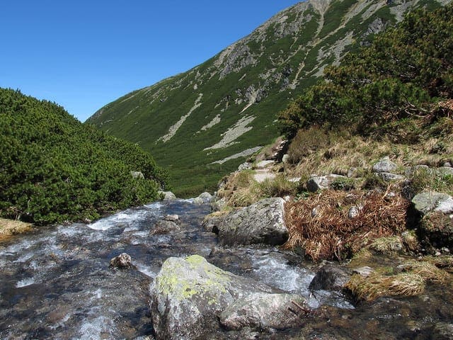
The example below loads the Fashion-MNIST dataset using the Keras API and creates a plot of the first nine images in the training dataset.

Running the example loads the Fashion-MNIST train and test dataset and prints their shape.

We can see that there are 60,000 examples in the training dataset and 10,000 in the test dataset and that images are indeed square with 28×28 pixels.

A plot of the first nine images in the dataset is also created showing that indeed the images are grayscale photographs of items of clothing.

Plot of a Subset of Images From the Fashion-MNIST Dataset

Model Evaluation Methodology

The Fashion MNIST dataset was developed as a response to the wide use of the MNIST dataset, that has been effectively “solved” given the use of modern convolutional neural networks.

Fashion-MNIST was proposed to be a replacement for MNIST, and although it has not been solved, it is possible to routinely achieve error rates of 10% or less. Like MNIST, it can be a useful starting point for developing and practicing a methodology for solving image classification using convolutional neural networks.

Instead of reviewing the literature on well-performing models on the dataset, we can develop a new model from scratch.

The dataset already has a well-defined train and test dataset that we can use.

In order to estimate the performance of a model for a given training run, we can further split the training set into a train and validation dataset. Performance on the train and validation dataset over each run can then be plotted to provide learning curves and insight into how well a model is learning the problem.

The Keras API supports this by specifying the “validation_data” argument to the model.fit() function when training the model, that will, in turn, return an object that describes model performance for the chosen loss and metrics on each training epoch.

In order to estimate the performance of a model on the problem in general, we can use k-fold cross-validation, perhaps 5-fold cross-validation. This will give some account of the model’s variance with both respect to differences in the training and test datasets and the stochastic nature of the learning algorithm. The performance of a model can be taken as the mean performance across k-folds, given with the standard deviation, that could be used to estimate a confidence interval if desired.

We can use the KFold class from the scikit-learn API to implement the k-fold cross-validation evaluation of a given neural network model. There are many ways to achieve this, although we can choose a flexible approach where the KFold is only used to specify the row indexes used for each split.

We will hold back the actual test dataset and use it as an evaluation of our final model.

How to Develop a Baseline Model

The first step is to develop a baseline model.

This is critical as it both involves developing the infrastructure for the test harness so that any model we design can be evaluated on the dataset, and it establishes a baseline in model performance on the problem, by which all improvements can be compared.

The design of the test harness is modular, and we can develop a separate function for each piece. This allows a given aspect of the test harness to be modified or inter-changed, if we desire, separately from the rest.

We can develop this test harness with five key elements. They are the loading of the dataset, the preparation of the dataset, the definition of the model, the evaluation of the model, and the presentation of results.

Load Dataset

We know some things about the dataset.

For example, we know that the images are all pre-segmented (e.g. each image contains a single item of clothing), that the images all have the same square size of 28×28 pixels, and that the images are grayscale. Therefore, we can load the images and reshape the data arrays to have a single color channel.

We also know that there are 10 classes and that classes are represented as unique integers.

We can, therefore, use a one hot encoding for the class element of each sample, transforming the integer into a 10 element binary vector with a 1 for the index of the class value. We can achieve this with the to_categorical() utility function.

The load_dataset() function implements these behaviors and can be used to load the dataset.

Prepare Pixel Data

We know that the pixel values for each image in the dataset are unsigned integers in the range between black and white, or 0 and 255.

We do not know the best way to scale the pixel values for modeling, but we know that some scaling will be required.

A good starting point is to normalize the pixel values of grayscale images, e.g. rescale them to the range [0,1]. This involves first converting the data type from unsigned integers to floats, then dividing the pixel values by the maximum value.

The prep_pixels() function below implement these behaviors and is provided with the pixel values for both the train and test datasets that will need to be scaled.

This function must be called to prepare the pixel values prior to any modeling.

Define Model

Next, we need to define a baseline convolutional neural network model for the problem.

The model has two main aspects: the feature extraction front end comprised of convolutional and pooling layers, and the classifier backend that will make a prediction.

For the convolutional front-end, we can start with a single convolutional layer with a small filter size (3,3) and a modest number of filters (32) followed by a max pooling layer. The filter maps can then be flattened to provide features to the classifier.

Given that the problem is a multi-class classification, we know that we will require an output layer with 10 nodes in order to predict the probability distribution of an image belonging to each of the 10 classes. This will also require the use of a softmax activation function. Between the feature extractor and the output layer, we can add a dense layer to interpret the features, in this case with 100 nodes.

All layers will use the ReLU activation function and the He weight initialization scheme, both best practices.

We will use a conservative configuration for the stochastic gradient descent optimizer with a learning rate of 0.01 and a momentum of 0.9. The categorical cross-entropy loss function will be optimized, suitable for multi-class classification, and we will monitor the classification accuracy metric, which is appropriate given we have the same number of examples in each of the 10 classes.

The define_model() function below will define and return this model.

Evaluate Model

After the model is defined, we need to evaluate it.

The model will be evaluated using 5-fold cross-validation. The value of k=5 was chosen to provide a baseline for both repeated evaluation and to not be too large as to require a long running time. Each test set will be 20% of the training dataset, or about 12,000 examples, close to the size of the actual test set for this problem.

The training dataset is shuffled prior to being split and the sample shuffling is performed each time so that any model we evaluate will have the same train and test datasets in each fold, providing an apples-to-apples comparison.

We will train the baseline model for a modest 10 training epochs with a default batch size of 32 examples. The test set for each fold will be used to evaluate the model both during each epoch of the training run, so we can later create learning curves, and at the end of the run, so we can estimate the performance of the model. As such, we will keep track of the resulting history from each run, as well as the classification accuracy of the fold.

The evaluate_model() function below implements these behaviors, taking the training dataset as arguments and returning a list of accuracy scores and training histories that can be later summarized.

Present Results

Once the model has been evaluated, we can present the results.

There are two key aspects to present: the diagnostics of the learning behavior of the model during training and the estimation of the model performance. These can be implemented using separate functions.

First, the diagnostics involve creating a line plot showing model performance on the train and test set during each fold of the k-fold cross-validation. These plots are valuable for getting an idea of whether a model is overfitting, underfitting, or has a good fit for the dataset.

We will create a single figure with two subplots, one for loss and one for accuracy. Blue lines will indicate model performance on the training dataset and orange lines will indicate performance on the hold out test dataset. The summarize_diagnostics() function below creates and shows this plot given the collected training histories.

Next, the classification accuracy scores collected during each fold can be summarized by calculating the mean and standard deviation. This provides an estimate of the average expected performance of the model trained on this dataset, with an estimate of the average variance in the mean. We will also summarize the distribution of scores by creating and showing a box and whisker plot.

The summarize_performance() function below implements this for a given list of scores collected during model evaluation.

Complete Example

We need a function that will drive the test harness.

This involves calling all of the define functions.

We now have everything we need; the complete code example for a baseline convolutional neural network model on the MNIST dataset is listed below.

Running the example prints the classification accuracy for each fold of the cross-validation process. This is helpful to get an idea that the model evaluation is progressing.

Note: Your results may vary given the stochastic nature of the algorithm or evaluation procedure, or differences in numerical precision. Consider running the example a few times and compare the average outcome.

We can see that for each fold, the baseline model achieved an error rate below 10%, and in two cases 98% and 99% accuracy. These are good results.

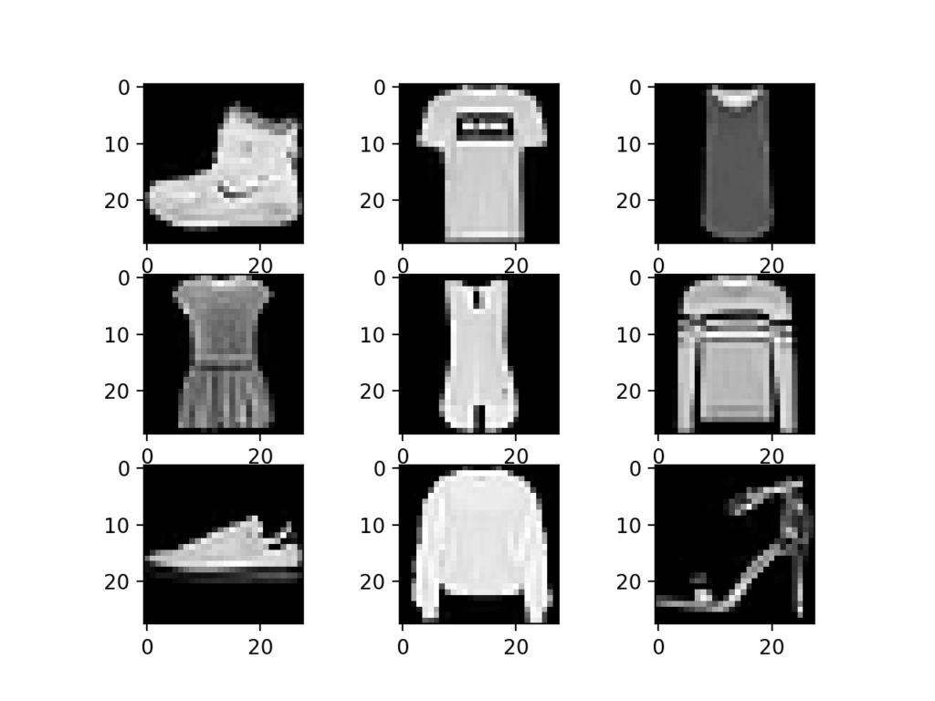
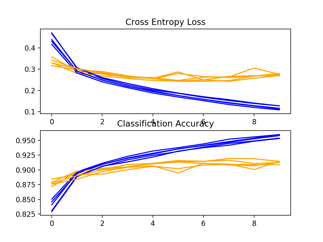
Next, a diagnostic plot is shown, giving insight into the learning behavior of the model across each fold.

In this case, we can see that the model generally achieves a good fit, with train and test learning curves converging. There may be some signs of slight overfitting.

Loss-and-Accuracy-Learning-Curves-for-the-Baseline-Model-on-the-Fashion-MNIST-Dataset-During-k-Fold-Cross-Validation

Next, the summary of the model performance is calculated. We can see in this case, the model has an estimated skill of about 96%, which is impressive.

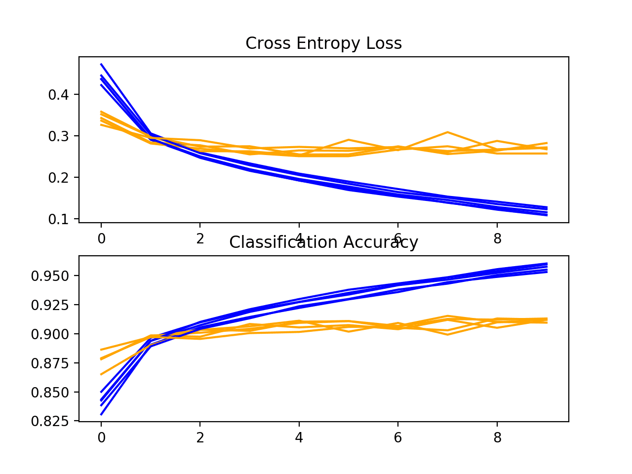
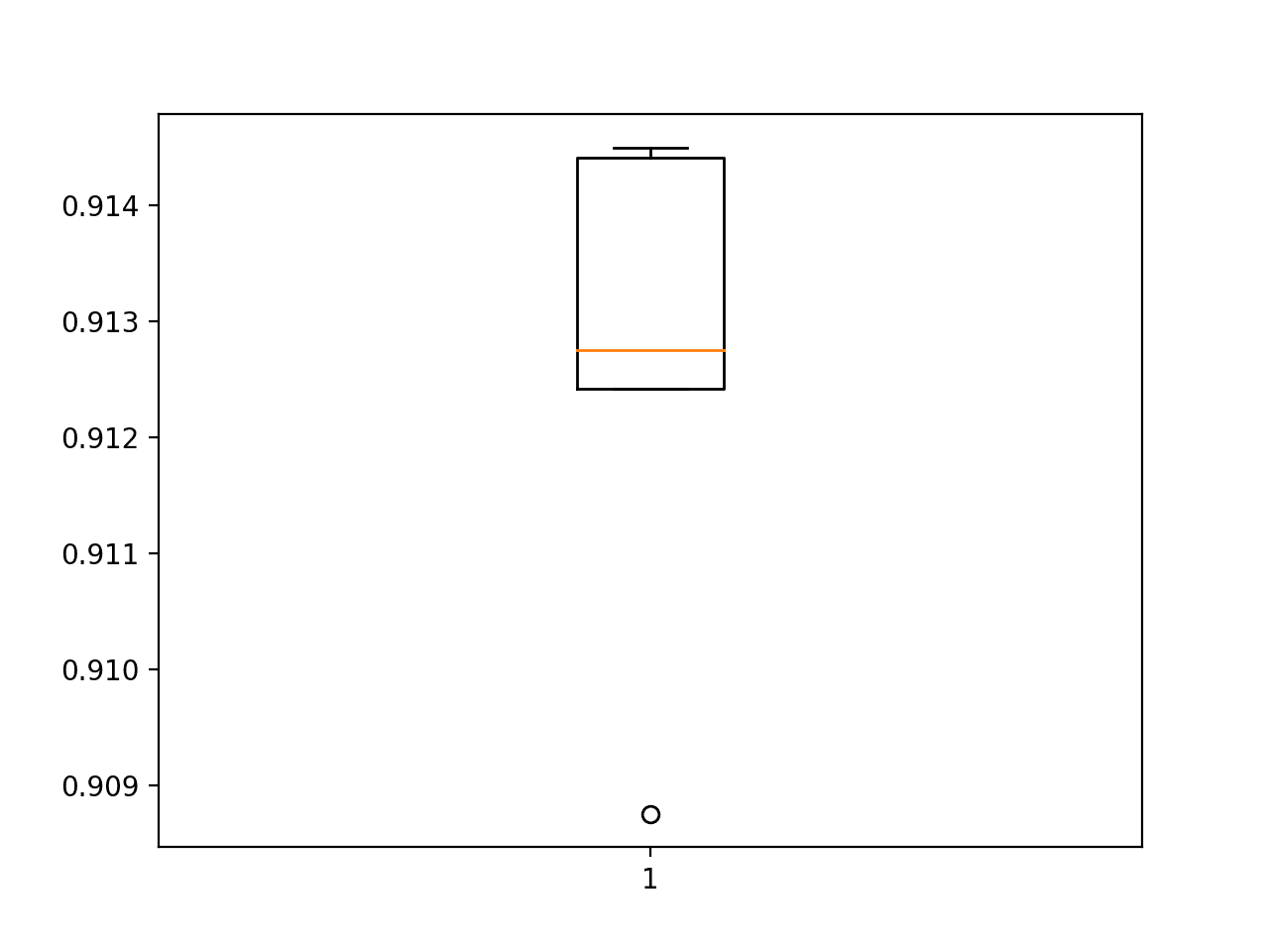
Finally, a box and whisker plot is created to summarize the distribution of accuracy scores.

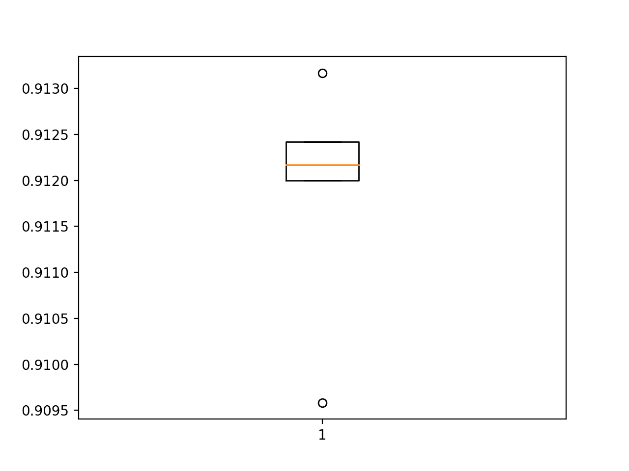
Box-and-Whisker-Plot-of-Accuracy-Scores-for-the-Baseline-Model-on-the-Fashion-MNIST-Dataset-Evaluated-Using-k-Fold-Cross-Validation

As we would expect, the distribution spread across the low-nineties.

We now have a robust test harness and a well-performing baseline model.

How to Develop an Improved Model

There are many ways that we might explore improvements to the baseline model.

We will look at areas that often result in an improvement, so-called low-hanging fruit. The first will be a change to the convolutional operation to add padding and the second will build on this to increase the number of filters.

Padding Convolutions

Adding padding to the convolutional operation can often result in better model performance, as more of the input image of feature maps are given an opportunity to participate or contribute to the output

By default, the convolutional operation uses ‘valid‘ padding, which means that convolutions are only applied where possible. This can be changed to ‘same‘ padding so that zero values are added around the input such that the output has the same size as the input.

The full code listing including the change to padding is provided below for completeness.

Running the example again reports model performance for each fold of the cross-validation process.

Note: Your results may vary given the stochastic nature of the algorithm or evaluation procedure, or differences in numerical precision. Consider running the example a few times and compare the average outcome.

We can see perhaps a small improvement in model performance as compared to the baseline across the cross-validation folds.

A plot of the learning curves is created. As with the baseline model, we may see some slight overfitting. This could be addressed perhaps with the use of regularization or the training for fewer epochs.

Loss-and-Accuracy-Learning-Curves-for-the-Same-Padding-on-the-Fashion-MNIST-Dataset-During-k-Fold-Cross-Validation

Next, the estimated performance of the model is presented, showing performance with a very slight decrease in the mean accuracy of the model, 91.257% as compared to 91.187% with the baseline model.

This may or may not be a real effect as it is within the bounds of the standard deviation. Perhaps more repeats of the experiment could tease out this fact.

Box-and-Whisker-Plot-of-Accuracy-Scores-for-Same-Padding-on-the-Fashion-MNIST-Dataset-Evaluated-Using-k-Fold-Cross-Validation

Increasing Filters

An increase in the number of filters used in the convolutional layer can often improve performance, as it can provide more opportunity for extracting simple features from the input images.

This is especially relevant when very small filters are used, such as 3×3 pixels.

In this change, we can increase the number of filters in the convolutional layer from 32 to double that at 64. We will also build upon the possible improvement offered by using ‘same‘ padding.

The full code listing including the change to padding is provided below for completeness.

Running the example reports model performance for each fold of the cross-validation process.

Note: Your results may vary given the stochastic nature of the algorithm or evaluation procedure, or differences in numerical precision. Consider running the example a few times and compare the average outcome.

The per-fold scores may suggest some further improvement over the baseline and using same padding alone.

A plot of the learning curves is created, in this case showing that the models still have a reasonable fit on the problem, with a small sign of some of the runs overfitting.

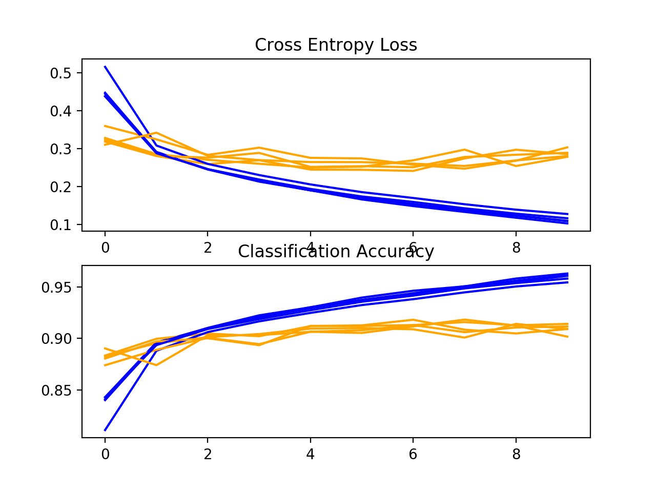
Loss-and-Accuracy-Learning-Curves-for-the-More-Filters-and-Padding-on-the-Fashion-MNIST-Dataset-During-k-Fold-Cross-Validation

Next, the estimated performance of the model is presented, showing a small improvement in performance as compared to the baseline from 90.913% to 91.257%.

Again, the change is still within the bounds of the standard deviation, and it is not clear whether the effect is real.

How to Finalize the Model and Make Predictions

The process of model improvement may continue for as long as we have ideas and the time and resources to test them out.

At some point, a final model configuration must be chosen and adopted. In this case, we will keep things simple and use the baseline model as the final model.

First, we will finalize our model, but fitting a model on the entire training dataset and saving the model to file for later use. We will then load the model and evaluate its performance on the hold out test dataset, to get an idea of how well the chosen model actually performs in practice. Finally, we will use the saved model to make a prediction on a single image.

Save Final Model

A final model is typically fit on all available data, such as the combination of all train and test dataset.

In this tutorial, we are intentionally holding back a test dataset so that we can estimate the performance of the final model, which can be a good idea in practice. As such, we will fit our model on the training dataset only.

Once fit, we can save the final model to an h5 file by calling the save() function on the model and pass in the chosen filename.

Note: saving and loading a Keras model requires that the h5py library is installed on your workstation.

The complete example of fitting the final model on the training dataset and saving it to file is listed below.

After running this example, you will now have a 1.2-megabyte file with the name ‘final_model.h5‘ in your current working directory.

Evaluate Final Model

We can now load the final model and evaluate it on the hold out test dataset.

This is something we might do if we were interested in presenting the performance of the chosen model to project stakeholders.

The model can be loaded via the load_model() function.

The complete example of loading the saved model and evaluating it on the test dataset is listed below.

Running the example loads the saved model and evaluates the model on the hold out test dataset.

The classification accuracy for the model on the test dataset is calculated and printed.

Note: Your results may vary given the stochastic nature of the algorithm or evaluation procedure, or differences in numerical precision. Consider running the example a few times and compare the average outcome.

In this case, we can see that the model achieved an accuracy of 90.990%, or just less than 10% classification error, which is not bad.

Make Prediction

We can use our saved model to make a prediction on new images.

The model assumes that new images are grayscale, they have been segmented so that one image contains one centered piece of clothing on a black background, and that the size of the image is square with the size 28×28 pixels.

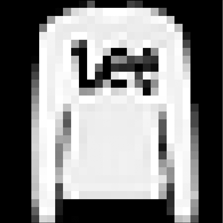
Below is an image extracted from the MNIST test dataset. You can save it in your current working directory with the filename ‘sample_image.png‘.

Sample Clothing (Pullover)

• Download Image (sample_image.png)

We will pretend this is an entirely new and unseen image, prepared in the required way, and see how we might use our saved model to predict the integer that the image represents. For this example, we expect class “2” for “Pullover” (also called a jumper).

First, we can load the image, force it to be grayscale format, and force the size to be 28×28 pixels. The loaded image can then be resized to have a single channel and represent a single sample in a dataset. The load_image() function implements this and will return the loaded image ready for classification.

Importantly, the pixel values are prepared in the same way as the pixel values were prepared for the training dataset when fitting the final model, in this case, normalized.

Next, we can load the model as in the previous section and call the predict_classes() function to predict the clothing in the image.

The complete example is listed below.

Running the example first loads and prepares the image, loads the model, and then correctly predicts that the loaded image represents a pullover or class ‘2’.

Extensions

This section lists some ideas for extending the tutorial that you may wish to explore.

• Regularization. Explore how adding regularization impacts model performance as compared to the baseline model, such as weight decay, early stopping, and dropout.
• Tune the Learning Rate. Explore how different learning rates impact the model performance as compared to the baseline model, such as 0.001 and 0.0001.
• Tune Model Depth. Explore how adding more layers to the model impact the model performance as compared to the baseline model, such as another block of convolutional and pooling layers or another dense layer in the classifier part of the model.

If you explore any of these extensions, I’d love to know.
Post your findings in the comments below.

Further Reading

This section provides more resources on the topic if you are looking to go deeper.

APIs

• Keras Datasets API
• Keras Datasets Code
• sklearn.model_selection.KFold API

Articles

• Fashion-MNIST GitHub Repository

Summary

In this tutorial, you discovered how to develop a convolutional neural network for clothing classification from scratch.

Specifically, you learned:

• How to develop a test harness to develop a robust evaluation of a model and establish a baseline of performance for a classification task.
• How to explore extensions to a baseline model to improve learning and model capacity.
• How to develop a finalized model, evaluate the performance of the final model, and use it to make predictions on new images.

Do you have any questions?
Ask your questions in the comments below and I will do my best to answer.

Develop Deep Learning Models for Vision Today!

Develop Your Own Vision Models in Minutes

...with just a few lines of python code

Discover how in my new Ebook:
Deep Learning for Computer Vision

It provides self-study tutorials on topics like:
classification, object detection (yolo and rcnn), face recognition (vggface and facenet), data preparation and much more...

Finally Bring Deep Learning to your Vision Projects

Skip the Academics. Just Results.

See What's Inside